Backward Euler method for the equations of motion arising in Oldroyd model of order one with nonsmooth initial data

Abstract

In this paper, a backward Euler method combined with finite element discretization in spatial direction is discussed for the equations of motion arising in the $2D$ Oldroyd model of viscoelastic fluids of order one with the forcing term independent of time or in $L^{\infty}$ in time. It is shown that the estimates of the discrete solution in Dirichlet norm is bounded uniformly in time. Optimal a priori error estimate in ${\bf L}^{2}$-norm is derived for the discrete problem with non-smooth initial data. This estimate is shown to be uniform in time, under the assumption of uniqueness condition. Finally, we present some numerical results to validate our theoretical results.

Key Words. Oldroyd fluid of order one, backward Euler method, uniform in time bound, optimal and uniform error estimates, non-smooth initial data.

1 Introduction

In this paper, we consider fully-discrete approximations to the equations of motion arising in the Oldroyd fluids (see Oldroyd [19]) of order one:

(1.1) $$~{}~{}\frac{\partial{\bf u}}{\partial t}+{\bf u}\cdot\nabla{\bf u}-\mu\Delta{\bf u}-\int_{0}^{t}\beta(t-\tau)\Delta{\bf u}(\tau)\,d\tau+\nabla p={\bf f},~{}~{}~{}~{}~{}\mbox{in}~{}\Omega,~{}t>0$$

with incompressibility condition

(1.2) $$\nabla\cdot{\bf u}=0,~{}~{}~{}~{}~{}\mbox{on}~{}\Omega,~{}t>0,$$

and initial and boundary conditions

(1.3) $${\bf u}(x,0)={\bf u}_{0}~{}~{}\mbox{in}~{}\Omega,~{}~{}~{}{\bf u}=0,~{}~{}\mbox{on}~{}\partial\Omega,~{}t\geq 0.$$

Here, $\Omega$ is a bounded domain in $\mathbb{R}^{2}$ with boundary $\partial\Omega$, $\mu=2\kappa\lambda^{-1}>0$, the kernel $\beta(t)=\gamma\exp(-\delta t),~{}\gamma=2\lambda^{-1}(\nu-\kappa\lambda^{-1})>0$ and $\delta=\lambda^{-1}>0$, where $\nu>0$ is the kinematic coefficient of viscosity, $\lambda>0$ is the relaxation time and $\kappa>0$ is the retardation time. Unknowns ${\bf u}$ and $p$ represent the velocity and the pressure of the fluid, respectively. Further, the forcing term ${\bf f}$ and initial velocity ${\bf u}_{0}$ are given functions in their respective domains of definition. For more details on the model, we refer to [19].

The model has been studied for more than three decades now; for early works and, for a brief introduction on the continuous and semi-discrete cases, we refer to [12, 7, 23] and references, therein. For recent and other notable works, we refer to [8, 9, 30, 31, 32, 33, 1, 15, 16, 17, 29] and references, therein.

Our present investigation is a continuation of our works in [7] and [24]. In [7], a priori estimates and regularity results for the solution pair $\{{\bf u},p\}$ of (1.1)-(1.3) are established under realistically assumed data and when ${\bf f},{\bf f}_{t}\in L^{\infty}(\mathbb{R}_{+};{\bf L}^{2}(\Omega))$. Further, optimal error estimates for the velocity and for the pressure are derived for the semidiscrete Galerkin approximations and these results are shown to be uniform under uniqueness condition. In this work, a completely discrete scheme based on backward Euler method is developed and analyzed for the problem (1.1)-(1.3). With $k$ as uniform time-step size, $t_{n}=nk$ as $n$th time level and $t_{N}=Nk$ as the final time, we denote ${\bf U}^{n}$ as the approximation of semi-discrete solution ${\bf u}_{h}$ at $t=t_{n}$ and fully-discrete approximation of ${\bf u}$ at $t=t_{n}$. We analyze the error due to the approximation ${\bf U}^{n}$ in light of non-smooth initial data and present optimal order error estimates. Before we discuss our main result and highlight the technical difficulties in its proof, we would first like to have a look at the available literature in this direction.

Literature for the fully-discrete approximation to the problem (1.1)-(1.3) is limited. In [2], Akhmatov and Oskolkov have discussed stable and convergent finite difference schemes for the problem (1.1)-(1.3). On the other hand, Pani et al., in [24], have considered a linearized backward Euler method to discretize in time direction only keeping spatial direction continuous and have used semi-group theoretic approach to establish a priori error estimates. The following time discrete error bounds are proved in [24]: (for $0<\alpha<\min\{\delta,\lambda_{1}\}$, $\lambda_{1}$ is the smallest positive eigenvalue of the Stokes operator)

$$\|{\bf u}(t_{n})-{\bf U}^{n}\|\leq Ce^{-\alpha t_{n}}k,~{}~{}\|{\bf u}(t_{n})-{\bf U}^{n}\|_{1}\leq Ce^{-\alpha t_{n}}k(t_{n}^{-1/2}+\log\frac{1}{k}),$$

for smooth initial data, i.e., ${\bf u}_{0}\in{\bf H}^{2}(\Omega)\cap{\bf J}_{1}$ (see, ${\bf J}_{1}$ in Section 2) and for zero forcing term (${\bf f}\equiv 0$). In [28], Wang et al. have extended this work to non-zero forcing function. They have used energy arguments, along with uniqueness condition to obtain for fully discrete solution ${\bf U}^{n}$, the following uniform error estimates

$$\|{\bf u}(t_{n})-{\bf U}^{n}\|\leq C(h^{2}+k),~{}~{}(\tau^{*})^{1/2}\|{\bf u}(t_{n})-{\bf U}^{n}\|_{1}\leq C(h+k),$$

where $\tau^{*}(t_{n})=\min\{1,t_{n}\}$ again for smooth data. In [8], Guo et al. have worked with a second-order time discretization scheme based on Crank-Nicolson/Adams-Bashforth as part of fully discrete analysis and have derived optimal error estimate under smooth initial data.

In the present work, we examine on the backward Euler method and prove the following (see, Theorem 5.1), when ${\bf u}_{0}\in{\bf H}_{0}^{1}(\Omega)$ :

$$\|{\bf u}_{h}(t_{n})-{\bf U}^{n}\|\leq K_{n}t_{n}^{-1/2}k\big{(}1+\log\frac{1}{k}\big{)}^{1/2},~{}~{}1\leq n\leq N<+\infty,$$

where $K_{n}>0$ is the error constant that depends only on the given data and, in particular, is independent of both $h$ and $k$. But it grows exponentially with time, that is, $K_{n}\sim O(e^{t_{n}})$ and therefore, the above error estimate is local (in time). Under uniqueness condition, we have shown the error to be uniformly bounded as $t\to+\infty$, see Section $6$.

These results are proved for nonsmooth initial data, that is, under realistically assumed regularity on the exact solution of the problem (1.1)-(1.3). For example, Lemma 3.2 says that $\|{\bf u}_{h}(t)\|_{2}$ and $\|{\bf u}_{ht}\|$ are of $O(t^{-1/2})$. As in [7], this breakdown at $t=0$ is a major bottle-neck in our error analysis. To illustrate our point, consider ${\bf u}_{0}\in{\bf H}_{0}^{1}(\Omega)\cap{\bf H}^{2}(\Omega)$ (smooth initial data). Then, the error ${\bf e}_{n}={\bf U}^{n}-{\bf u}_{h}(t_{n})$ satisfies the following estimate (see, Lemma $4.2$ of [28]):

$$\|{\bf e}_{n}\|\sim O(k),~{}~{}1\leq n\leq N,$$

Following similar argument but now with ${\bf u}_{0}\in{\bf H}_{0}^{1}(\Omega)$, we would only obtain

$$\|{\bf e}_{n}\|\sim O(k^{1/2}\big{(}1+\log\frac{1}{k}\big{)}^{1/2}),~{}~{}1\leq n\leq N.$$

The loss in the order of $k$, in fact, is due to the singularity of the higher-order norms of the solution at $t=0$. The standard technique, in such cases, is to multiply by a weight $t^{r},~{}r\in\mathbb{N}$ to compensate for this singularity, thereby, recovering full order of convergence. But in our case, a direct application of this technique fails due to the presence of the memory term. Note that the kernel $\beta$ present in the equation (1.1) has a certain positivity property (see Lemma $2.1$ of [7]) and we choose our quadrature rule to conform with it, see (4.1). This is crucial to our analysis. But when we opt for weighted Sobolev norm with a weight $t^{r},~{}r\in\mathbb{N}$, it nullifies the positivity property of our quadrature rule. The main effort of this work is to overcome this difficulty and to recover optimal fully discrete error estimate for the velocity. This requires borrowing certain tools from error analysis of linear parabolic integro-differential equations with non-smooth data (see; [20, 21, 27]), like, the summation technique (we call it here ”hat operator”, see (5.35)), which adds to the technicality.

The error analysis has been carried out by splitting the error into two parts such as error due to linearized part and error due to nonlinear part and then analyzing both part separately. Our approach has two advantages. Firstly, we notice that the exponential increase of the error bound (as $t\to+\infty$) is due to the nonlinear part, since the other part is uniformly bounded as $t\to+\infty$, see, lemma 5.5. Secondly, for non-smooth initial data, the uniform error estimate (which has been done in Section $6$), can only be obtained by splitting the error likewise.

Apart from the error analysis, we have also established uniform (in time) Dirichlet norm for the fully discrete solution ${\bf U}^{n}$, meaning $\|\nabla{\bf U}^{n}\|,~{}1\leq n\leq N$ remains bounded as $t_{N}\to+\infty$. It is crucial for the long-time stability of the implicit scheme. In case of Navier-Stokes, the proof of the Dirichlet norm of ${\bf U}^{n}$, which is valid for all time, involves applying discrete version of the uniform Gronwall’s Lemma (see, Lemma 2.6 from [26]). In our case, it is difficult to apply the uniform Gronwall’s Lemma due to the presence of the quadrature term. Hence, we resort to a new way of looking into the ideas behind the uniform Gronwall’s Lemma to establish our result.

We now summarize our main results as follows:

• Uniform bound in time for the fully discrete solution in the Dirichlet norm depicting long term stability.

• New uniform estimates for the error associated with fully discrete linearized problem.

• Local optimal error estimates for the discrete velocity in ${\bf L}^{2}$-norm.

• Optimal global fully discrete error estimates under the uniqueness assumption.

At this stage, it is useful to compare our results with the results derived in [24]. In [24], only discretization in time keeping spatial variables continuous has been analyzed using semigroup theory approach for the homogeneous problem, that is, ${\bf f}=0$, and error estimates are obtained under the assumption of ${\bf u}_{0}\in{\bf H}^{2}\cap{\bf J}_{1}$. But the present analysis deals with the fully discrete scheme, uses energy arguments and establishes the optimal error estimates for the nonhomogeneous problem (1.1)-(1.3) with nonsmooth initial data, that is, ${\bf u}_{0}\in{\bf H}_{0}^{1}\cap{\bf J}_{1}$. In both papers, a common thread is the time weighted estimates.

Henceforward, we will use $K$ and $C$ as positive generic constants, where $K$ would depend on the given data.

The remaining part of this paper is organized as follows. In Section $2$, we discuss some notations, basic assumptions and weak formulations of the problem (1.1)-(1.3). Section $3$ deals with a brief description of a semi-discrete Galerkin finite element method. Section $4$ is devoted to backward Euler method. Optimal error bounds are obtained for the velocity and for the pressure for the problem (1.1)-(1.3) with non-smooth initial data, in Section $5$, whereas, in Section $6$, these bounds are shown to be uniform in time, under uniqueness condition. In Section $7$, we present some numerical experiments whose results confirm our theoretical findings. Finally, we summarize our results in Section $8$.

2 Preliminaries

For our subsequent use we denote by bold face letters the $\mathbb{R}^{2}$-valued function space such as

$${\bf H}_{0}^{1}=[H_{0}^{1}(\Omega)]^{2},~{}~{}~{}{\bf L}^{2}=[L^{2}(\Omega)]^{2}~{}~{}\mbox{and}~{}~{}~{}{\bf H}^{m}=[H^{m}(\Omega)]^{2},$$

where $H^{m}(\Omega)$ is the standard Hilbert Sobolev space of order $m$. Note that ${\bf H}^{1}_{0}$ is equipped with a norm

$$\|\nabla{\bf v}\|=\left(\sum_{i,j=1}^{2}(\partial_{j}v_{i},\partial_{j}v_{i})\right)^{1/2}=\left(\sum_{i=1}^{2}(\nabla v_{i},\nabla v_{i})\right)^{1/2}.$$

Further, we introduce below, divergence free function spaces:

$${\bf J}_{1} =\{\mbox{\boldmath$\phi$}\in{\bf H}_{0}^{1}:\nabla\cdot\mbox{\boldmath$\phi$}=0\},$$

$${\bf J} =\{\mbox{\boldmath$\phi$}\in{\bf L}^{2}:\nabla\cdot\mbox{\boldmath$\phi$}=0~{}\mbox{in}~{}\Omega,~{}\mbox{\boldmath$\phi$}\cdot{\bf n}|_{\partial\Omega}=0~{}~{}\mbox{holds weakly}\},$$

where ${\bf n}$ is the outward normal to the boundary $\partial\Omega$ and $\mbox{\boldmath$\phi$}\cdot{\bf n}|_{\partial\Omega}=0$ should be understood in the sense of trace in ${\bf H}^{-1/2}(\partial\Omega)$, see [25]. Let $H^{m}/\mathbb{R}$ be the quotient space consisting of equivalence classes of elements of $H^{m}$ differing by constants, which is equipped with norm $\|p\|_{H^{m}/\mathbb{R}}=\inf_{c\in\mathbb{R}}\|p+c\|_{m}$. For any Banach space $X$, let $L^{p}(0,T;X)$ denote the space of measurable $X$-valued functions $\phi$ on $(0,T),~{}0<T\leq+\infty$, such that

$$\int_{0}^{T}\|\mbox{\boldmath$\phi$}(t)\|^{p}_{X}~{}dt<+\infty~{}~{}~{}\mbox{if}~{}~{}1\leq p<+\infty,$$

and for $p=+\infty$

$${\displaystyle{ess\sup_{0<t<T}}}\|\mbox{\boldmath$\phi$}(t)\|_{X}<+\infty.$$

Through out this paper, we make the following assumptions:
(${\bf A1}$). For ${\bf g}\in{\bf L}^{2}(\Omega)$, let the unique pair of solutions $\{{\bf v},q\}\in{\bf J}_{1}\times L^{2}(\Omega)/\mathbb{R}$ for the steady state Stokes problem

$$-\Delta{{\bf v}}+\nabla q={\bf{g}},~{}\nabla\cdot{\bf v}=0~{}{\mbox{i}n}~{}\Omega~{}~{}\mbox{and}~{}~{}{\bf v}|_{\partial\Omega}=0,$$

satisfy the following regularity result

$$\|{\bf v}\|_{2}+\|q\|_{H^{1}(\Omega)/\mathbb{R}}\leq C\|{\bf g}\|.$$

(${\bf A2}$). The initial velocity ${\bf u}_{0}$ and the external force ${\bf f}$ satisfy, for positive constant $M_{0},$

$${\bf u}_{0}\in{\bf J}_{1},~{}{\bf f},{\bf f}_{t}\in L^{\infty}(\mathbb{R}_{+};{\bf L}^{2}(\Omega))~{}~{}\mbox{with}~{}~{}\|{\bf u}_{0}\|_{1}\leq M_{0},~{}~{}{\displaystyle{\sup_{t>0}}}\big{\{}\|{\bf f}\|,\|{\bf f}_{t}\|\big{\}}\leq M_{0}.$$

With $P$ as orthogonal projection of ${\bf L}^{2}(\Omega)$ onto ${\bf J}$, we set ${\tilde{\Delta}}=P\Delta$ as the Stokes operator. Then, (${\bf A1}$) implies

$$\|{\bf v}\|_{2}\leq C\|{\tilde{\Delta}}{\bf v}\|,~{}~{}\|\nabla{\bf v}\|^{2}\leq\lambda_{1}^{-1}\|{\tilde{\Delta}}{\bf v}\|^{2},~{}~{}\forall~{}{\bf v}\in{\bf J}_{1}\cap{\bf H}^{2}(\Omega),\mbox{ and ~{}}\|{\bf v}\|^{2}\leq\lambda_{1}^{-1}\|\nabla{\bf v}\|^{2},~{}~{}\forall~{}{\bf v}\in{\bf J}_{1},$$

where $\lambda_{1}$ is the least positive eigenvalue of the Stokes operator, see [13].

Before going to the details, let us introduce the weak formulation of (1.1)-(1.3): Find a pair of functions $\{{\bf u}(t),p(t)\}\in{\bf H}_{0}^{1}\times L^{2}/\mathbb{R},~{}t>0,$ such that

$$({\bf u}_{t},\mbox{\boldmath$\phi$})+\mu(\nabla{\bf u},\nabla\mbox{\boldmath$\phi$})+({\bf u}\cdot\nabla{\bf u},\mbox{\boldmath$\phi$})+\int_{0}^{t}\beta(t-s)(\nabla{\bf u}(s),\nabla\mbox{\boldmath$\phi$})ds-(p,\nabla\cdot\mbox{\boldmath$\phi$}) =({\bf f},\mbox{\boldmath$\phi$}),~{}~{}\forall\mbox{\boldmath$\phi$}\in{\bf H}_{0}^{1}$$

$$(\nabla\cdot{\bf u},\chi) =0,~{}~{}\forall\chi\in L^{2}.$$

Equivalently, find ${\bf u}(\cdot,t)\in{\bf J}_{1}$ such that

$$({\bf u}_{t},\mbox{\boldmath$\phi$})+\mu(\nabla{\bf u},\nabla\mbox{\boldmath$\phi$})+({\bf u}\cdot\nabla{\bf u},\mbox{\boldmath$\phi$})+\int_{0}^{t}\beta(t-s)(\nabla{\bf u}(s),\nabla\mbox{\boldmath$\phi$})ds=({\bf f},\mbox{\boldmath$\phi$}),~{}~{}\forall\mbox{\boldmath$\phi$}\in{\bf J}_{1},~{}t>0.$$

Now, we present below, the discrete Gronwall’s Lemma. For a proof, see, [11, 22]:

Lemma 2.1 (discrete Gronwall’s Lemma).

Let $k,B$ and $\{a_{i},b_{i},c_{i},d_{i}\}_{i\in\mathbb{N}}$ be non-negative numbers such that

$$a_{n}+k\sum_{i=1}^{n}b_{i}\leq B+k\sum_{i=1}^{n-1}c_{i}+k\sum_{i=1}^{n-1}d_{i}a_{i},~{}~{}\forall n\geq 1.$$

Then,

$$a_{n}+k\sum_{i=1}^{n}b_{i}\leq\Big{\{}B+k\sum_{i=1}^{n-1}c_{i}\Big{\}}\exp\Big{(}k\sum_{i=1}^{n-1}d_{i}\Big{)},~{}~{}\forall n\geq 1.$$

3 Semidiscrete Galerkin Approximations

From now on, we denote $h$ with $0<h<1$ to be a real positive discretization parameter tending to zero. Let ${\bf H}_{h}$ and $L_{h}$ be finite dimensional subspaces of ${\bf H}_{0}^{1}$ and $L^{2}$, respectively, approximating the velocity vector and the pressure. Assume the following approximation properties for the spaces ${\bf H}_{h}$ and $L_{h}$:
${\bf(B1)}$ For each ${\bf w}\in{\bf H}_{0}^{1}\cap{\bf H}^{2}$ and $q\in H^{1}/\mathbb{R}$ there exist approximations $i_{h}w\in{\bf H}_{h}$ and $j_{h}q\in L_{h}$ such that

$$\|{\bf w}-i_{h}{\bf w}\|+h\|\nabla({\bf w}-i_{h}{\bf w})\|\leq Ch^{2}\|{\bf w}\|_{2},~{}~{}~{}~{}\|q-j_{h}q\|_{L^{2}/\mathbb{R}}\leq Ch\|q\|_{H^{1}/\mathbb{R}}.$$

Further, suppose that the following inverse hypothesis holds for ${\bf w}_{h}\in{\bf H}_{h}$:

$$\|\nabla{\bf w}_{h}\|\leq Ch^{-1}\|{\bf w}_{h}\|.$$

To define the Galerkin approximations, set for ${\bf v},{\bf w},\mbox{\boldmath$\phi$}\in{\bf H}_{0}^{1}$,

$$a({\bf v},\mbox{\boldmath$\phi$})=(\nabla{\bf v},\nabla\mbox{\boldmath$\phi$})~{}~{}~{}\mbox{and}~{}~{}~{}b({\bf v},{\bf w},\mbox{\boldmath$\phi$})=\frac{1}{2}({\bf v}\cdot\nabla{\bf w},\mbox{\boldmath$\phi$})-\frac{1}{2}({\bf v}\cdot\nabla\mbox{\boldmath$\phi$},{\bf w}).$$

Note that the operator $b(\cdot,\cdot,\cdot)$ preserves the antisymmetric property of the original nonlinear term, that is,

$$b({\bf v}_{h},{\bf w}_{h},{\bf w}_{h})=0,\;\;\;\forall{\bf v}_{h},{\bf w}_{h}\in{{\bf H}}_{h}.$$

Now the semidiscrete Galerkin formulation reads as: Find $({\bf u}_{h}(t),p_{h}(t))\in{\bf H}_{h}\times L_{h}$ such that ${\bf u}_{h}(0)={\bf u}_{0h}$

(3.1) $$({\bf u}_{ht},\mbox{\boldmath$\phi$}_{h})+\mu a({\bf u}_{h},\mbox{\boldmath$\phi$}_{h})+ b({\bf u}_{h},{\bf u}_{h},\mbox{\boldmath$\phi$}_{h})+a({\bf u}_{h,{\beta}},\mbox{\boldmath$\phi$}_{h})-(p_{h},\nabla\cdot\mbox{\boldmath$\phi$}_{h})=({\bf f},\mbox{\boldmath$\phi$}_{h}),$$

$$(\nabla\cdot{\bf u}_{h},\chi_{h})=0,$$

for $\mbox{\boldmath$\phi$}_{h}\in{\bf H}_{h},~{}\chi_{h}\in L_{h}$ and for $t>0$. Here ${\bf u}_{0h}\in{\bf H}_{h}$ is a suitable approximation of ${\bf u}_{0}\in{\bf J}_{1}$ and

$${\bf u}_{h,{\beta}}(t)=\int_{0}^{t}\beta(t-s){\bf u}_{h}(s)~{}ds.$$

In order to consider a discrete space analogous to ${\bf J}_{1}$, we impose the discrete incompressibility condition on ${\bf H}_{h}$ and call it as ${\bf J}_{h}$. We define ${\bf J}_{h}$ as

$${\bf J}_{h}:=\{v_{h}\in{\bf H}_{h}:(\chi_{h},\nabla\cdot v_{h})=0,~{}~{}\forall\chi_{h}\in L_{h}\}.$$

Note that ${\bf J}_{h}$ is not a subspace of ${\bf J}_{1}$. With ${\bf J}_{h}$ as above, we now introduce an equivalent Galerkin formulation. Find ${\bf u}_{h}(t)\in{\bf J}_{h}$ such that ${\bf u}_{h}(0)={\bf u}_{0h}$ and for $t>0$

(3.2) $$({\bf u}_{ht},\mbox{\boldmath$\phi$}_{h})+\mu a({\bf u}_{h},\mbox{\boldmath$\phi$}_{h})+a({\bf u}_{h,{\beta}},\mbox{\boldmath$\phi$}_{h})=-b({\bf u}_{h},{\bf u}_{h},\mbox{\boldmath$\phi$}_{h})+({\bf f},\mbox{\boldmath$\phi$}_{h}),~{}~{}\forall\mbox{\boldmath$\phi$}_{h}\in{\bf J}_{h}.$$

Since ${\bf J}_{h}$ is finite dimensional, the problem (3.2) leads to a system of nonlinear integro-differential equations. For global existence of a unique solution ${\bf u}_{h}$ of (3.2), we refer to [23]. Then $\ p_{h}$ is recovered from (3.1). Uniqueness (of $p_{h}$) is obtained in the quotient space $L_{h}/N_{h}$, where

$$N_{h}=\{q_{h}\in L_{h}:(q_{h},\nabla\cdot\mbox{\boldmath$\phi$}_{h})=0,~{}~{}\forall\mbox{\boldmath$\phi$}_{h}\in{\bf H}_{h}\}.$$

The norm on $L_{h}/N_{h}$ is given by

$$\|q_{h}\|_{L^{2}/N_{h}}={\displaystyle{\inf_{\chi_{h}\in N_{h}}}}\|q_{h}+\chi_{h}\|.$$

For continuous dependence of the discrete pressure $p_{h}(t)\in L_{h}/N_{h}$ on the discrete velocity ${\bf u}_{h}(t)\in{\bf J}_{h}$, we assume the following discrete inf-sup (LBB) condition for the finite dimensional spaces ${\bf H}_{h}$ and $L_{h}$:
${\bf(B2^{\prime})}$ For every $q_{h}\in L_{h}$, there exists a non-trivial function $\mbox{\boldmath$\phi$}_{h}\in{\bf H}_{h}$ such that

$$|(q_{h},\nabla\cdot\mbox{\boldmath$\phi$}_{h})|\geq C\|\nabla\mbox{\boldmath$\phi$}_{h}\|\|q_{h}\|_{L^{2}/N_{h}}.$$

Moreover, we also assume that the following approximation property holds true for ${\bf J}_{h}$.
${\bf(B2)}$ For every ${\bf w}\in{\bf J}_{1}\cap{\bf H}^{2},$ there exists an approximation $r_{h}{\bf w}\in{\bf J_{h}}$ such that

$$\|{\bf w}-r_{h}{\bf w}\|+h\|\nabla({\bf w}-r_{h}{\bf w})\|\leq Ch^{2}\|{\bf w}\|_{2}.$$

This is a less restrictive condition than (${\bf B2^{\prime}}$) and it has been used to derive the following properties of the $L^{2}$ projection $P_{h}:{\bf L}^{2}\mapsto{\bf J}_{h}$. We state below these results without proof. For a proof, see [13].

$$\|\mbox{\boldmath$\phi$}-P_{h}\mbox{\boldmath$\phi$}\|+h\|\nabla P_{h}\mbox{\boldmath$\phi$}\| \leq Ch\|\nabla\mbox{\boldmath$\phi$}\|,~{}~{}\text{for}~{}\mbox{\boldmath$\phi$}\in{\bf J}_{h},$$

$$\|\mbox{\boldmath$\phi$}-P_{h}\mbox{\boldmath$\phi$}\|+h\|\nabla(\mbox{\boldmath$\phi$}-P_{h}\mbox{\boldmath$\phi$})\| \leq Ch^{2}\|{\tilde{\Delta}}\mbox{\boldmath$\phi$}\|,~{}~{}\text{for}~{}\mbox{\boldmath$\phi$}\in{\bf J}_{1}\cap{\bf H}^{2}.$$

We now define the discrete Laplace operator $\Delta_{h}:{\bf H}_{h}\mapsto{\bf H}_{h}$ through the bilinear form $a(\cdot,\cdot)$ as

$$a({\bf v}_{h},\mbox{\boldmath$\phi$}_{h})=(-\Delta_{h}{\bf v}_{h},\mbox{\boldmath$\phi$}),~{}~{}\forall{\bf v}_{h},\mbox{\boldmath$\phi$}_{h}\in{\bf H}_{h}.$$

Denoting the orthogonal projection of $L^{2}$ onto $J$ as $P$, we define the Stokes operator as ${\tilde{\Delta}}=P\Delta$ and set its discrete version as ${\tilde{\Delta}}_{h}=P_{h}\Delta_{h}$. The restriction of ${\tilde{\Delta}}_{h}$ to ${\bf J}_{h}$ is invertible and we denote the inverse by ${\tilde{\Delta}}_{h}^{-1}$. Since $-{\tilde{\Delta}}_{h}$ is self-adjoint and positive definite, we define discrete Sobolev norms on ${\bf J}_{h}$ as follows:

$$\|{\bf v}_{h}\|_{r}=\|(-{\tilde{\Delta}}_{h})^{r/2}{\bf v}_{h}\|,~{}~{}{\bf v}_{h}\in{\bf J}_{h},~{}r\in\mathbb{R}.$$

We note that in particular $\|{\bf v}_{h}\|_{0}=\|{\bf v}_{h}\|$ and $\|{\bf v}_{h}\|_{1}=\|\nabla{\bf v}_{h}\|$ for ${\bf v}_{h}\in{\bf J}_{h}$, and $\|\cdot\|_{2}$ and $\|{\tilde{\Delta}}_{h}\cdot\|$ are equivalent norms on ${\bf J}_{h}$. For further detail, we refer to [13, 14].

Remark 3.1.

To avoid confusion as to whether $\|\cdot\|_{1}$ means standard or discrete Sobolev norm, we follow the convention that if ${\bf v}$ belongs to ${\bf J}_{h}$ then $\|{\bf v}\|_{1}$ represents ${\bf v}$ in discrete Soboelev norm, otherwise it is the standard Sobolev norm.

Below we present some estimates of the nonlinear operator $b$ for our subsequent use. The proofs of these estimates are well known and can be found in the literature based on Navier-Stokes equations (e.g., see [14, (3.7)]).

Lemma 3.1.

Suppose conditions (${\bf A1}$), (${\bf B1}$) and (${\bf B2}$) are satisfied. Then there exists a positive constant $C$ such that for ${\bf v},{\bf w},\mbox{\boldmath$\phi$}\in{\bf H}_{h}$, the following holds:

(3.3) $$|({\bf v}\cdot\nabla{\bf w},\mbox{\boldmath$\phi$})|\leq C\left\{\begin{array}[]{l}\|{\bf v}\|^{1/2}\|\nabla{\bf v}\|^{1/2}\|\nabla{\bf w}\|^{1/2}\|\Delta_{h}{\bf w}\|^{1/2}\|\mbox{\boldmath$\phi$}\|,\\ \|{\bf v}\|^{1/2}\|\Delta_{h}{\bf v}\|^{1/2}\|\nabla{\bf w}\|\|\mbox{\boldmath$\phi$}\|,\\ \|{\bf v}\|^{1/2}\|\nabla{\bf v}\|^{1/2}\|\nabla{\bf w}\|\|\mbox{\boldmath$\phi$}\|^{1/2}\|\nabla\mbox{\boldmath$\phi$}\|^{1/2},\\ \|{\bf v}\|\|\nabla{\bf w}\|\|\mbox{\boldmath$\phi$}\|^{1/2}\|\Delta_{h}\mbox{\boldmath$\phi$}\|^{1/2},\\ \|{\bf v}\|\|\nabla{\bf w}\|^{1/2}\|\Delta_{h}{\bf w}\|^{1/2}\|\mbox{\boldmath$\phi$}\|^{1/2}\|\nabla\mbox{\boldmath$\phi$}\|^{1/2}.\end{array}\right.$$

Examples of subspaces ${\bf H}_{h}$ and $L_{h}$ satisfying assumptions (${\bf B1}$), (${\bf B2}^{\prime}$), and (${\bf B2}$) can be found in [3, 4, 5].
We present below a Lemma that deals with higher order estimates of ${\bf u}_{h},$ which will be useful in the error analysis of backward Euler method for non-smooth data.

Lemma 3.2.

Let $0<\alpha<\min\{\delta,\lambda_{1}\mu\}$ and let (${\bf A1}$), (${\bf A2}$), (${\bf B1}$) and (${\bf B2}$) be satisfied. Moreover, let ${\bf u}_{h}(0)\in{\bf J}_{h}$. Then ${\bf u}_{h},$ the solutions of the semidiscrete Oldroyd problem (3.2), satisfies the following a priori estimates:

(3.4) $$\tau^{*}\|{\bf u}_{h}\|_{2}^{2}+(\tau^{*})^{r+1}(t)\|{\bf u}_{ht}\|_{r}^{2} \leq K,~{}~{}~{}~{}r\in\{0,1\},$$

(3.5) $$e^{-2\alpha t}\int_{0}^{t}e^{2\alpha s}(\tau^{*})^{r}(s)\|{\bf u}_{hs}\|^{2}_{r}\,ds \leq K,~{}~{}~{}~{}r\in\{0,1,2\},$$

(3.6) $$e^{-2\alpha t}\int_{0}^{t}e^{2\alpha s}(\tau^{*})^{r+1}(s)\|{\bf u}_{hss}\|_{r-1}^{2}~{}ds \leq K,~{}~{}~{}~{}r\in\{-1,0,1\},$$

where $\tau^{*}(t)=\min\{1,t\}$ and $K$ depends on the given data, but not on time $t$.

Proof.

The estimates (3.4)-(3.5) can be proved as in the continuous case, see [7]. The final estimate follows in a similar manner. For the sake of completeness, we provide a sketch here. Differentiate (3.2) to find that, for $\mbox{\boldmath$\phi$}_{h}\in{\bf J}_{h},$

$$({\bf u}_{htt},\mbox{\boldmath$\phi$}_{h})+\mu a({\bf u}_{ht},\mbox{\boldmath$\phi$}_{h}) +\beta(0)a({\bf u}_{h},\mbox{\boldmath$\phi$}_{h})-\delta\int_{0}^{t}\beta(t-s)a({\bf u}_{h}(s),\mbox{\boldmath$\phi$}_{h})~{}ds$$

(3.7) $$=-b({\bf u}_{ht},{\bf u}_{h},\mbox{\boldmath$\phi$}_{h})-b({\bf u}_{h},{\bf u}_{ht},\mbox{\boldmath$\phi$}_{h})+({\bf f}_{t},\mbox{\boldmath$\phi$}_{h}).$$

Put $\mbox{\boldmath$\phi$}_{h}=(\tau^{*})^{2}(t)e^{2\alpha t}{\bf u}_{htt}$ in (3) to obtain

$$(\tau^{*})^{2}(t)e^{2\alpha t}\|{\bf u}_{htt}\|^{2}+\mu a({\bf u}_{ht},(\tau^{*})^{2}(t)e^{2\alpha t}{\bf u}_{htt})=(\tau^{*})^{2}(t)e^{2\alpha t}\Big{(}-\gamma a({\bf u}_{h},{\bf u}_{htt})+\delta\int_{0}^{t}\beta(t-s)a({\bf u}_{h}(s),{\bf u}_{htt})~{}ds$$

(3.8) $$-b({\bf u}_{ht},{\bf u}_{h},{\bf u}_{htt})-b({\bf u}_{h},{\bf u}_{ht},{\bf u}_{htt})+({\bf f}_{t},{\bf u}_{htt})\Big{)}.$$

The second term on the left hand side of (3) can be written as

$$\mu\ a({\bf u}_{ht},(\tau^{*})^{2}(t)e^{2\alpha t}{\bf u}_{htt}) =\frac{\mu}{2}(\tau^{*})^{2}(t)e^{2\alpha t}\frac{d}{dt}\|{\bf u}_{ht}\|_{1}^{2}$$

$$=\frac{\mu}{2}\frac{d}{dt}\big{(}(\tau^{*})^{2}(t)e^{2\alpha t}\|{\bf u}_{ht}\|_{1}^{2}\big{)}-\mu\big{(}\alpha(\tau^{*})^{2}(t)+\tau^{*}(t)\frac{d}{dt}(\tau^{*})(t)\big{)}e^{2\alpha t}\|{\bf u}_{ht}\|_{1}^{2}.$$

Next use the Cauchy-Schwarz inequality in first, second and last terms on the right hand side of (3) to obtain

$$(\tau^{*})^{2}(t)e^{2\alpha t}\|{\bf u}_{htt}\|^{2}+ \frac{\mu}{2}\frac{d}{dt}\big{(}(\tau^{*})^{2}(t)e^{2\alpha t}\|{\bf u}_{ht}\|_{1}^{2}\big{)}\leq\big{(}\alpha(\tau^{*})^{2}(t)+\tau^{*}(t)\big{)}e^{2\alpha t}\|{\bf u}_{ht}\|_{1}^{2}$$

$$+\gamma(\tau^{*})^{2}(t)e^{2\alpha t}\|{\bf u}_{h}\|_{2}\|{\bf u}_{htt}\|+\delta(\tau^{*})^{2}(t)e^{2\alpha t}\int_{0}^{t}\beta(t-s)\|{\bf u}_{h}(s)\|_{2}\|{\bf u}_{htt}\|~{}ds$$

(3.9) $$+(\tau^{*})^{2}(t)e^{2\alpha t}\big{(}|b({\bf u}_{ht},{\bf u}_{h},{\bf u}_{htt})|+|b({\bf u}_{h},{\bf u}_{ht},{\bf u}_{htt})|+\|f_{t}\|\|{\bf u}_{htt}\|\big{)}.$$

Here, without loss of generality, we have assumed that $\frac{d}{dt}\tau^{*}(t)\leq 1$. To avoid confusion we can always first derive these estimate in the interval $(0,1)$ and then in $(1,t),~{}t>1$. For the nonlinear terms, we first note that

(3.10) $$b({\bf u}_{ht},{\bf u}_{h},{\bf u}_{htt})=\frac{1}{2}({\bf u}_{ht}\cdot\nabla{\bf u}_{h},{\bf u}_{htt})-\frac{1}{2}({\bf u}_{ht}\cdot\nabla{\bf u}_{htt},{\bf u}_{h}).$$

But we can rewrite the second term as follows: (with notations $D_{i}=\frac{\partial}{\partial x_{i}}$ and ${\bf v}=(v^{1},v^{2})$)

(3.11) $$({\bf u}_{ht}\cdot\nabla{\bf u}_{htt},{\bf u}_{h}) =\sum_{i,j=1}^{2}\int_{\Omega}u_{ht}^{i}D_{i}(u_{htt}^{j})u_{h}^{j}d{\bf x}$$

$$=-\sum_{i,j=1}^{2}\int_{\Omega}D_{i}(u_{ht}^{i})u_{htt}^{j}u_{h}^{j}d{\bf x}-\sum_{i,j=1}^{2}\int_{\Omega}u_{ht}^{i}u_{htt}^{j}D_{i}(u_{h}^{j})d{\bf x}$$

$$=-((\nabla\cdot{\bf u}_{ht}){\bf u}_{htt},{\bf u}_{h})-({\bf u}_{ht}\cdot\nabla{\bf u}_{h},{\bf u}_{htt}).$$

Use (3.11) in (3.10) and now use (3.3) to estimate the nonlinear terms.

(3.12) $$|b({\bf u}_{ht},{\bf u}_{h},{\bf u}_{htt})|+|b({\bf u}_{h},{\bf u}_{ht},{\bf u}_{htt})|\leq\frac{1}{4}\|{\bf u}_{htt}\|^{2}+K\|{\bf u}_{ht}\|_{1}^{2}\|{\bf u}_{h}\|_{2}^{2}.$$

Incorporate (3.12) in (3) and, apply Young’s inequality and kickback argument. Then integrate with respect to time. The resulting double integral is estimated similar to $(3.26)$ of [7]. Now using (3.4)-(3.5) we can easily deduce that

$$(\tau^{*})^{2}\|{\bf u}_{ht}\|_{1}^{2}+\mu e^{-2\alpha t}\int_{0}^{t}(\tau^{*})^{2}(s)e^{2\alpha s}\|{\bf u}_{hss}\|^{2}~{}ds\leq K.$$

We set $\mbox{\boldmath$\phi$}_{h}=-\tau^{*}(t)e^{2\alpha t}{\tilde{\Delta}}_{h}^{-1}{\bf u}_{htt}$ in (3). From (3.3) we see that

$$b({\bf u}_{ht},{\bf u}_{h},{\tilde{\Delta}}_{h}^{-1}{\bf u}_{htt})\leq K\|{\bf u}_{ht}\|^{1/2}\|{\bf u}_{ht}\|_{1}^{1/2}\|{\bf u}_{h}\|_{1}\|{\bf u}_{htt}\|_{-1}$$

and therefore

$$\mu\frac{d}{dt}(\tau^{*}(t)e^{2\alpha t}\|{\bf u}_{ht}\|^{2})+\tau^{*}(t)e^{2\alpha t}\|{\bf u}_{htt}\|_{-1}^{2}\leq\big{(}2\alpha\tau^{*}(t)+1\big{)}e^{2\alpha t}\|{\bf u}_{ht}\|_{1}^{2}+C(\mu,\gamma)\tau^{*}(t)e^{2\alpha t}\|\nabla{\bf u}_{h}\|^{2}+2\|{\bf f}_{t}\|^{2}$$

$$+C(\mu,\delta)(\int_{0}^{t}\beta(t-s)e^{\alpha t}\|{\tilde{\Delta}}_{h}{\bf u}_{h}(s)\|~{}ds)^{2}+C(\mu)\tau^{*}(t)e^{2\alpha t}\Big{(}\|\nabla{\bf u}_{h}\|^{2}\|{\bf u}_{ht}\|^{2}+\|\nabla{\bf u}_{ht}\|^{2}(1+\|{\bf u}_{h}\|\|\nabla{\bf u}_{h}\|)\Big{)}.$$

Integrate with respect to time and multiply by $e^{-2\alpha t}$ to conclude

$$\tau^{*}(t)\|{\bf u}_{ht}\|^{2}+\mu e^{-2\alpha t}\int_{0}^{t}\tau^{*}(s)e^{2\alpha s}\|{\bf u}_{hss}\|_{-1}^{2}ds\leq K.$$

Finally we set $\mbox{\boldmath$\phi$}_{h}=-e^{2\alpha t}{\tilde{\Delta}}_{h}^{2}{\bf u}_{htt}$ in (3) and proceed as above to arrive at

$$\|{\bf u}_{ht}\|_{-1}^{2}+\mu e^{-2\alpha t}\int_{0}^{t}e^{2\alpha s}\|{\bf u}_{hss}\|_{-2}^{2}ds\leq K.$$

This completes the rest of the proof. ∎

The following semi-discrete error estimates are proved in [7].

Theorem 3.1.

Let $\Omega$ be a convex polygon and let the conditions (${\bf A1}$)-(${\bf A2}$) and (${\bf B1}$)-(${\bf B2}$) be satisfied. Further, let the discrete initial velocity ${\bf u}_{0h}\in{\bf J}_{h}$ with ${\bf u}_{0h}=P_{h}{\bf u}_{0},$ where ${\bf u}_{0}\in{\bf J}_{1}.$ Then, there exists a positive constant $K$ such that for $0<T<+\infty$ with $t\in(0,T]$

$$\|({\bf u}-{\bf u}_{h})(t)\|+h\|\nabla({\bf u}-{\bf u}_{h})(t)\|\leq Ke^{Kt}h^{2}t^{-1/2}.$$

Moreover under the assumption of the uniqueness condition, that is,

(3.13) $$\frac{N}{\nu^{2}}\|{\bf f}\|_{\infty}<1~{}~{}~{}\mbox{and}~{}~{}N=\sup_{{\bf u},{\bf v},{\bf w}\in{\bf H}_{0}^{1}(\Omega)}\frac{b({\bf u},{\bf v},{\bf w})}{\|\nabla{\bf u}\|\|\nabla{\bf v}\|\|\nabla{\bf w}\|},$$

where $\nu=\mu+\frac{\gamma}{\delta}$ and $\|{\bf f}\|_{\infty}:=\|{\bf f}\|_{L^{\infty}(\mathbb{R}_{+};{\bf L}^{2}(\Omega))}$, we have the following uniform estimate:

$$\|({\bf u}-{\bf u}_{h})(t)\|\leq Kh^{2}t^{-1/2}.$$

4 Backward Euler Method

This section deals with fully discrete scheme based on backward Euler method, existence of unique discrete solutions and some uniform in time bounds. For time discretization, let $k=\frac{T}{N}$ be the time step with $t_{n}=nk,~{}n\geq 0$, $N$ is a positive integer. We define for a sequence $\{\mbox{\boldmath$\phi$}^{n}\}_{n\geq 0}\subset{\bf J}_{h},$ the backward difference quotient

$$\partial_{t}\mbox{\boldmath$\phi$}^{n}=\frac{1}{k}(\mbox{\boldmath$\phi$}^{n}-\mbox{\boldmath$\phi$}^{n-1}).$$

For any continuous function ${\bf v}(t)$ we set ${\bf v}_{n}={\bf v}(t_{n})$. Since backward Euler method is of first order in time, we choose the right rectangle rule to approximate the integral term in (3.2).

$$q_{r}^{n}(\mbox{\boldmath$\phi$})=k\sum_{j=1}^{n}\beta_{nj}\phi^{j}\approx\int_{0}^{t_{n}}\beta(t_{n}-s)\mbox{\boldmath$\phi$}(s)~{}ds,$$

where $\beta_{nj}=\beta(t_{n}-t_{j}).$ With $w_{nj}=k\beta_{nj}$, it is observed that the the right rectangle rule is positive in the sense that

(4.1) $$k\sum_{i=1}^{n}q_{r}^{i}(\phi)\phi^{i}=k\sum_{i=1}^{n}\sum_{j=0}^{i}\omega_{ij}\phi^{j}\phi^{i}\geq 0,~{}~{}~{}~{}\phi=(\phi^{0},\cdots,\phi^{N})^{T}.$$

For details, see, McLean and Thomée [18]. The error incurred due to right rectangle rule in approximating the integral term is

(4.2) $$\varepsilon_{r}^{n}(\phi) =\int_{0}^{t_{n}}\beta(t_{n}-s)\mbox{\boldmath$\phi$}(s)~{}ds-k\sum_{j=1}^{n}\beta_{nj}\phi^{j}$$

$$=-\sum_{j=1}^{n}\int_{t_{j-1}}^{t_{j}}(s-t_{j-1})\frac{\partial}{\partial s}(\beta(t_{n}-s)\mbox{\boldmath$\phi$}(s))~{}ds\leq k\sum_{j=1}^{n}\int_{t_{j-1}}^{t_{j}}\Big{|}\frac{\partial}{\partial s}(\beta(t_{n}-s)\mbox{\boldmath$\phi$}(s))\Big{|}~{}ds.$$

We present here a discrete version of integration by parts for our subsequent use. For sequences $\{a_{i}\}$ and $\{b_{i}\}$ of real numbers, the following summation by parts holds

(4.3) $$k\sum_{j=1}^{i}a_{j}b_{j}=a_{i}\widehat{b}_{i}-k\sum_{j=1}^{i-1}(\partial_{t}a_{j+1})\widehat{b}_{j},~{}~{}\mbox{ where }\widehat{b}_{i}=k\sum_{j=1}^{i}b_{j}.$$

Here, we observe that for sequences $\{a_{i}\}$ and $\{b_{i}\}$ of real numbers,

(4.4) $$\sigma_{i}(a_{i},\partial_{t}b_{i})=\partial_{t}(\sigma_{i}(a_{i},b_{i}))-\sigma_{i}(\partial_{t}a_{i},b_{i})-(\partial_{t}\sigma_{i})(a_{i},b_{i}),$$

where, $\sigma_{n}=e^{2\alpha t_{n}}\tau^{*}(t_{n})$ and $\tau^{*}(t_{n})=\min\{1,t_{n}\}$. Now, the backward Euler scheme for the semidiscrete Oldroyd problem (3.1) is to find $\{{\bf U}^{n}\}_{1\leq n\leq N}\in{\bf H}_{h}$ and $\{P^{n}\}_{1\leq n\leq N}\in L_{h}$ as solutions of the recursive nonlinear algebraic equations ($1\leq n\leq N$):

(4.5) $$\left\{\begin{array}[]{l}(\partial_{t}{\bf U}^{n},\mbox{\boldmath$\phi$}_{h})+\mu a({\bf U}^{n},\mbox{\boldmath$\phi$}_{h})+a(q_{r}^{n}({\bf U}),\mbox{\boldmath$\phi$}_{h})=(P^{n},\nabla\cdot\mbox{\boldmath$\phi$}_{h})+({\bf f}^{n},\mbox{\boldmath$\phi$}_{h})-b({\bf U}^{n},{\bf U}^{n},\mbox{\boldmath$\phi$}_{h}),~{}~{}~{}\forall\ \mbox{\boldmath$\phi$}_{h}\in{\bf H}_{h},\\ (\nabla\cdot{\bf U}^{n},\chi_{h})=0,~{}~{}~{}\forall\ \chi_{h}\in L_{h},~{}~{}~{}n\geq 0.\end{array}\right.$$

We choose ${\bf U}^{0}={\bf u}_{0h}=P_{h}{\bf u}_{0}.$ On the other hand, for $\mbox{\boldmath$\phi$}_{h}\in{\bf J}_{h}$ we seek $\{{\bf U}^{n}\}_{1\leq n\leq N}\in{\bf J}_{h}$ such that

(4.6) $$(\partial_{t}{\bf U}^{n},\mbox{\boldmath$\phi$}_{h})+\mu a({\bf U}^{n},\mbox{\boldmath$\phi$}_{h})+a(q_{r}^{n}({\bf U}),\mbox{\boldmath$\phi$}_{h})=({\bf f}^{n},\mbox{\boldmath$\phi$}_{h})-b({\bf U}^{n},{\bf U}^{n},\mbox{\boldmath$\phi$}_{h}),~{}~{}~{}\forall\mbox{\boldmath$\phi$}_{h}\in{\bf J}_{h}.$$

Using variant of the Brouwer fixed point theorem and standard uniqueness argument, one can show that the discrete problem (4.6) is well-posed. For a proof, we refer to [6]. Below, we prove a priori bounds for the discrete solutions $\{{\bf U}^{n}\}_{1\leq n\leq N}.$ We note here that since the bounds proved below are independent of $n,~{}1\leq n\leq N$, these bounds are uniform in time, that is, they are still valid as the final time $t_{N}\to+\infty$.

Lemma 4.1.

Let $\alpha_{0}>0$ be such that for $0<\alpha<\alpha_{0}$

(4.7) $$1+\big{(}\frac{\mu\lambda_{1}}{2}\big{)}k\geq e^{\alpha k}.$$

Then, with $0<\alpha<\min\{\alpha_{0},\delta,\frac{\mu\lambda_{1}}{2}\}$ the discrete solution ${\bf U}^{n},~{}1\leq n\leq N$ of (4.6) satisfies the following estimate:

$$\|{\bf U}^{n}\|^{2}+\frac{\mu}{2}e^{-2\alpha t_{n}}ke^{-\alpha k}\sum_{i=1}^{n}e^{2\alpha t_{i}}\|\nabla{\bf U}^{i}\|^{2}\leq C\Big{(}e^{-2\alpha t_{n}}\|{\bf U}^{0}\|^{2}+\frac{1}{\mu\lambda_{1}}\|{\bf f}\|_{\infty}^{2}\Big{)},$$

where $\|{\bf f}\|_{\infty}=\|{\bf f}\|_{L^{\infty}(\mathbb{R}_{+};{\bf L}^{2}(\Omega))}$.

Proof.

Although the proof is similar to [24, Lemma 9], we have provided a sketch below for the sake of completeness. Setting $\tilde{{\bf U}}^{n}=e^{\alpha t_{n}}{\bf U}^{n},$ we rewrite (4.6), for $\mbox{\boldmath$\phi$}_{h}\in{\bf J}_{h},$ as

(4.8) $$e^{\alpha t_{n}}(\partial_{t}{\bf U}^{n},\mbox{\boldmath$\phi$}_{h})+\mu a(\tilde{{\bf U}}^{n},\mbox{\boldmath$\phi$}_{h})+e^{-\alpha t_{n}}b(\tilde{{\bf U}}^{n},\tilde{{\bf U}}^{n},\mbox{\boldmath$\phi$}_{h})+e^{\alpha t_{n}}a(q_{r}^{n}({\bf U}),\mbox{\boldmath$\phi$}_{h})=(\tilde{{\bf f}}^{n},\mbox{\boldmath$\phi$}_{h}).$$

Note that

$$e^{\alpha t_{n}}\partial_{t}{\bf U}^{n}=e^{\alpha k}\partial_{t}\tilde{{\bf U}}^{n}-\Big{(}\frac{e^{\alpha k}-1}{k}\Big{)}\tilde{{\bf U}}^{n}.$$

On substituting this in (4.8) and then multiplying the resulting equation by $e^{-\alpha k},$ we obtain

$$(\partial_{t}\tilde{{\bf U}}^{n},\mbox{\boldmath$\phi$}_{h})-\Big{(}\frac{1-e^{-\alpha k}}{k}\Big{)}(\tilde{{\bf U}}^{n},\mbox{\boldmath$\phi$}_{h}) +e^{-\alpha k}\mu a(\tilde{{\bf U}}^{n},\mbox{\boldmath$\phi$}_{h})+e^{-\alpha t_{n+1}}b(\tilde{{\bf U}}^{n},\tilde{{\bf U}}^{n},\mbox{\boldmath$\phi$}_{h})$$

(4.9) $$+\gamma e^{-\alpha k}\sum_{i=1}^{n}e^{-(\delta-\alpha)(t_{n}-t_{i})}a(\tilde{{\bf U}}^{i},\mbox{\boldmath$\phi$}_{h})=e^{-\alpha k}(\tilde{{\bf f}}^{n},\mbox{\boldmath$\phi$}_{h}).$$

Observe that

$$(\partial_{t}\tilde{{\bf U}}^{n},\tilde{{\bf U}}^{n})=\frac{1}{k}(\tilde{{\bf U}}^{n}-\tilde{{\bf U}}^{n-1},\tilde{{\bf U}}^{n})\geq\frac{1}{2k}(\|\tilde{{\bf U}}^{n}\|^{2}-\|\tilde{{\bf U}}^{n-1}\|^{2})=\frac{1}{2}\partial_{t}\|\tilde{{\bf U}}^{n}\|^{2}$$

and that the nonlinear term vanishes, that is, $b(\tilde{{\bf U}}^{n},\tilde{{\bf U}}^{n},\tilde{{\bf U}}^{n})=0$.
Put $\mbox{\boldmath$\phi$}_{h}=\tilde{{\bf U}}^{i}$ in (4), for $n=i$ and use Poincaré inequality $\|\tilde{{\bf U}}^{i}\|^{2}\leq\frac{1}{\lambda_{1}}\|\nabla\tilde{{\bf U}}^{i}\|^{2}$ to obtain

(4.10) $$\frac{1}{2}\partial_{t}\|\tilde{{\bf U}}^{i}\|^{2}-\Big{(}\frac{1-e^{-\alpha k}}{k\lambda_{1}}\Big{)}\|\nabla\tilde{{\bf U}}^{i}\|^{2}+e^{-\alpha k}\mu\|\nabla\tilde{{\bf U}}^{i}\|^{2}+\gamma e^{-\alpha k}k\sum_{j=1}^{i}e^{-(\delta-\alpha)(t_{i}-t_{j})}a(\tilde{{\bf U}}^{j},\tilde{{\bf U}}^{i})=e^{-\alpha k}(\tilde{{\bf f}}^{i},\tilde{{\bf U}}^{i}).$$

The right-hand side of (4.10) can be estimated as

$$e^{-\alpha k}\|\tilde{{\bf f}}^{i}\|\|\tilde{{\bf U}}^{i}\|\leq\frac{1}{4}e^{-\alpha k}\mu\|\nabla\tilde{{\bf U}}^{i}\|^{2}+\frac{1}{\mu\lambda_{1}}e^{-\alpha k}\|\tilde{{\bf f}}^{i}\|^{2},$$

so as to obtain from (4.10)

(4.11) $$\partial_{t}\|\tilde{{\bf U}}^{i}\|^{2}+2e^{-\alpha k}\Big{(}\frac{3}{4}\mu-\big{(}\frac{e^{\alpha k}-1}{k\lambda_{1}}\big{)}\Big{)}\|\nabla\tilde{{\bf U}}^{i}\|^{2}+2\gamma e^{-\alpha k}k\sum_{j=1}^{i}e^{-(\delta-\alpha)(t_{i}-t_{j})}a(\tilde{{\bf U}}^{j},\tilde{{\bf U}}^{i})\leq\frac{2}{\mu\lambda_{1}}e^{-\alpha k}\|\tilde{{\bf f}}^{i}\|^{2}.$$

With $0<\alpha<\min\{\alpha_{0},\delta,\frac{\mu\lambda_{1}}{2}\},$ (4.7) is satisfied; which guarantees that $\frac{\mu}{2}\geq\frac{e^{\alpha k}-1}{k\lambda_{1}}.$ Now multiply (4.11) by $k$ and then sum over $i=1$ to $n.$ The resulting double sum is non-negative and hence we obtain

(4.12) $$\|\tilde{{\bf U}}^{n}\|^{2}+\frac{\mu}{2}ke^{-\alpha k}\sum_{i=1}^{n}\|\nabla\tilde{{\bf U}}^{i}\|^{2}\leq\|{\bf U}^{0}\|^{2}+\frac{2\|{\bf f}\|_{\infty}^{2}}{\mu\lambda_{1}}e^{-\alpha k}k\sum_{i=1}^{n}e^{2\alpha t_{i}}.$$

Note that using geometric series, we find, for some $k^{*}$ in $(0,k)$ that

(4.13) $$k\sum_{i=1}^{n}e^{2\alpha t_{i}}=e^{2\alpha k}\frac{k}{e^{2\alpha k}-1}e^{2\alpha t_{n}}=e^{2\alpha(k-k^{*})}e^{2\alpha t_{n}},$$

On substituting (4.13) in (4.12), multiply through out by $e^{-2\alpha t_{n}}$ to complete the rest of the proof.
∎

Remark 4.1.

In Lemma 4.1, such a choice of $\alpha_{0}>0$ is possible by choosing $\alpha_{0}<\frac{\log(1+\frac{\mu\lambda_{1}}{2}k)}{k}$. Note that for large $k>0$, $\alpha_{0}$ is small but as $k\to 0$, $\frac{\log(1+\frac{\mu\lambda_{1}}{2}k)}{k}\to\frac{\mu\lambda_{1}}{2}$. Thus, with $0<\alpha<\min\{\alpha_{0},\delta,\frac{\mu\lambda_{1}}{2}\}$, the result in Lemma 4.1 is valid.

In order to obtain uniform (in time) estimate for the discrete solution ${\bf U}^{n}$ in Dirichlet norm, we introduce the following notation:

(4.14) $${\bf U}^{n}_{\beta}=k\sum_{j=1}^{n}\beta_{nj}{\bf U}^{j},~{}n>0;~{}~{}{\bf U}^{0}_{\beta}=0,$$

and rewrite (4.6), for $\mbox{\boldmath$\phi$}_{h}\in{\bf J}_{h},$ as

(4.15) $$(\partial_{t}{\bf U}^{n},\mbox{\boldmath$\phi$}_{h})+\mu a({\bf U}^{n},\mbox{\boldmath$\phi$}_{h})+b({\bf U}^{n},{\bf U}^{n},\mbox{\boldmath$\phi$}_{h})+a({\bf U}^{n}_{\beta},\mbox{\boldmath$\phi$}_{h})=({\bf f}^{n},\mbox{\boldmath$\phi$}_{h}).$$

Note that

$${\bf U}^{n}_{\beta}=k\gamma{\bf U}^{n}+e^{-\delta k}{\bf U}^{n-1}_{\beta},$$

and therefore,

(4.16) $$\partial_{t}{\bf U}^{n}_{\beta}=\frac{1}{k}({\bf U}^{n}_{\beta}-{\bf U}^{n-1}_{\beta})=\frac{1}{k}{\bf U}^{n}_{\beta}-\frac{1}{k}e^{\delta k}({\bf U}^{n}_{\beta}-k\gamma{\bf U}^{n})=\gamma e^{\delta k}{\bf U}^{n}-\frac{(e^{\delta k}-1)}{k}{\bf U}^{n}_{\beta}.$$

Lemma 4.2.

Under the assumptions of Lemma 4.1, the discrete solution ${\bf U}^{n},~{}1\leq n\leq N$, of (4.6), satisfies the following uniform estimates:

(4.17) $$\|{\bf U}^{n}\|^{2}+\frac{e^{-\delta k}}{\gamma}\|\nabla{\bf U}^{n}_{\beta}\|^{2}\leq e^{-\alpha t_{n}}\|{\bf U}^{0}\|^{2}+\left(\frac{1-e^{-\alpha t_{n}}}{\alpha\mu\lambda_{1}}\right)\|{\bf f}\|^{2}_{\infty}=M_{11}^{2},$$

and

(4.18) $$k\sum_{n=m}^{m+l}\big{(}\mu\|\nabla{\bf U}^{n}\|^{2}+\frac{\delta}{\gamma}\|\nabla{\bf U}^{n}_{\beta}\|^{2}\big{)}\leq M_{11}^{2}+\frac{l}{\mu\lambda_{1}}\|{\bf f}\|^{2}_{\infty}=M_{12}^{2}(l),$$

where ${\bf U}^{n}_{\beta}$ is given by (4.14) and $m,l\in\mathbb{N}$.

Proof.

In view of (4.16), we find that

$$a({\bf U}^{n}_{\beta},{\bf U}^{n})=\frac{e^{-\delta k}}{\gamma}a({\bf U}^{n}_{\beta},\partial_{t}{\bf U}^{n}_{\beta})+\frac{(1-e^{-\delta k})}{k\gamma}\|\nabla{\bf U}^{n}_{\beta}\|^{2}.$$

Now take $\mbox{\boldmath$\phi$}_{h}={\bf U}^{n}$ in (4.15), for $n=i$, to find

(4.19) $$\partial_{t}\big{(}\|{\bf U}^{i}\|^{2}+\frac{e^{-\delta k}}{\gamma}\|\nabla{\bf U}^{i}_{\beta}\|^{2}\big{)}+2\mu\|\nabla{\bf U}^{i}\|^{2}+2\Big{(}\frac{e^{\delta k}-1}{k}\Big{)}\frac{e^{-\delta k}}{\gamma}\|\nabla{\bf U}^{i}_{\beta}\|^{2}\leq 2\|{\bf f}^{i}\|\|{\bf U}^{i}\|\leq\frac{1}{\mu\lambda_{1}}\|{\bf f}^{i}\|^{2}+\mu\|\nabla{\bf U}^{i}\|^{2}.$$

A use of the kick back Poincaré inequality $\mu\|\nabla{\bf U}^{i}\|^{2}\geq\mu\lambda_{1}\|{\bf U}^{i}\|^{2}$ yields

(4.20) $$\partial_{t}\big{(}\|{\bf U}^{i}\|^{2}+\frac{e^{-\delta k}}{\gamma}\|\nabla{\bf U}^{i}_{\beta}\|^{2}\big{)}+\mu\lambda_{1}\|{\bf U}^{i}\|^{2}+2\Big{(}\frac{e^{\delta k}-1}{k}\Big{)}\frac{e^{-\delta k}}{\gamma}\|\nabla{\bf U}^{i}_{\beta}\|^{2}\leq\frac{1}{\mu\lambda_{1}}\|{\bf f}^{i}\|^{2}.$$

Multiply the inequality (4.20) by $e^{\alpha t_{i-1}}$ and note that

(4.21) $$\partial_{t}(e^{\alpha t_{i}}\mbox{\boldmath$\phi$}^{i})=e^{\alpha t_{i-1}}\Big{\{}\partial_{t}\mbox{\boldmath$\phi$}^{i}+\frac{e^{\alpha k}-1}{k}\mbox{\boldmath$\phi$}^{i}\Big{\}}.$$

Therefore, we obtain from (4.20)

$$\partial_{t}\Big{(}e^{\alpha t_{i}}\big{(}\|{\bf U}^{i}\|^{2}+\frac{e^{-\delta k}}{\gamma}\|\nabla{\bf U}^{i}_{\beta}\|^{2}\big{)}\Big{)} +\Big{(}\mu\lambda_{1}-\frac{e^{\alpha k}-1}{k}\Big{)}e^{\alpha t_{i-1}}\|{\bf U}^{i}\|^{2}$$

$$+\Big{(}2\big{(}\frac{e^{\delta k}-1}{k}\big{)}-\big{(}\frac{e^{\alpha k}-1}{k}\big{)}\Big{)}\frac{e^{-\delta k}}{\gamma}e^{\alpha t_{i-1}}\|\nabla{\bf U}^{i}_{\beta}\|^{2}\leq\frac{e^{\alpha t_{i-1}}}{\mu\lambda_{1}}\|{\bf f}\|_{\infty}^{2}.$$

With $0<\alpha<\min\{\alpha_{0},\delta,\mu\lambda_{1}/2\}$, the last two terms on the left hand side become non-negative and hence, we drop it. Multiply by $k$ and sum over $1$ to $n$ and then multiply the resulting inequality by $e^{-\alpha t_{n}}.$ Observe that ${\bf U}^{0}_{\beta}=0$ by definition. This results in the first estimate (4.17). For the second estimate (4.18), we multiply (4.19) by $k,$ sum over $m$ to $m+l$ with $m,l\in\mathbb{N}$ and use (4.17) to complete the rest of the proof. ∎

Lemma 4.3.

Under the assumptions of Lemma 4.1, the discrete solution ${\bf U}^{n},~{}1\leq n\leq N$ of (4.6) satisfies the following uniform estimates:

$$\|\nabla{\bf U}^{n}\|^{2}+\frac{e^{-\delta k}}{\gamma}\|{\tilde{\Delta}}_{h}{\bf U}^{n}_{\beta}\|^{2}\leq K.$$

Proof.

Set $\mbox{\boldmath$\phi$}_{h}=-{\tilde{\Delta}}_{h}{\bf U}^{n}$ in (4.15) and as in the Lemma 4.2, we now obtain

$$\partial_{t}\big{(}\|\nabla{\bf U}^{n}\|^{2}+\frac{e^{-\delta k}}{\gamma}\|{\tilde{\Delta}}_{h}{\bf U}^{n}_{\beta}\|^{2}\big{)}+2\mu\|{\tilde{\Delta}}_{h}{\bf U}^{n}\|^{2}+2\big{(}\frac{e^{\delta k}-1}{k}\big{)}\frac{e^{-\delta k}}{\gamma}\|{\tilde{\Delta}}_{h}{\bf U}^{n}_{\beta}\|^{2}$$

(4.22) $$\leq 2\|{\bf f}^{n}\|\|{\tilde{\Delta}}_{h}{\bf U}^{n}\|+2|b({\bf U}^{n},{\bf U}^{n},-{\tilde{\Delta}}_{h}{\bf U}^{n})|.$$

Use Lemma 3.1, 4.2 and the Young inequality to estimate the nonlinear term as

$$2|b({\bf U}^{n},{\bf U}^{n},-{\tilde{\Delta}}_{h}{\bf U}^{n})| \leq 2C\|{\bf U}^{n}\|^{1/2}\|\nabla{\bf U}^{n}\|^{1/2}\|\nabla{\bf U}^{n}\|^{1/2}\|{\tilde{\Delta}}_{h}{\bf U}^{n}\|^{1/2}\|{\tilde{\Delta}}_{h}{\bf U}^{n}\|$$

$$\leq(\frac{9/2}{\mu})^{3}M_{11}^{2}\|\nabla{\bf U}^{n}\|^{4}+\frac{\mu}{3}\|{\tilde{\Delta}}_{h}{\bf U}^{n}\|^{2}$$

Thus we obtain from (4)

$$\partial_{t}\big{(}\|\nabla{\bf U}^{n}\|^{2}+\frac{e^{-\delta k}}{\gamma}\|{\tilde{\Delta}}_{h}{\bf U}^{n}_{\beta}\|^{2}\big{)}+\frac{4\mu}{3}\|{\tilde{\Delta}}_{h}{\bf U}^{n}\|^{2}+2\big{(}\frac{e^{\delta k}-1}{k}\big{)}\frac{e^{-\delta k}}{\gamma}\|{\tilde{\Delta}}_{h}{\bf U}^{n}_{\beta}\|^{2}$$

(4.23) $$\leq\frac{3}{\mu}\|{\bf f}\|_{\infty}^{2}+(\frac{9/2}{\mu})^{3}M_{11}^{2}\|\nabla{\bf U}^{n}\|^{4}.$$

Choose $\gamma_{0}>0$,

(4.24) $$\gamma_{0}\|\nabla{\bf U}^{n}\|^{2}=\gamma_{0}({\bf U}^{n},-{\tilde{\Delta}}_{h}{\bf U}^{n})\leq\frac{\mu}{3}\|{\tilde{\Delta}}_{h}{\bf U}^{n}\|^{2}+\frac{3}{4\mu}\gamma_{0}^{2}\|{\bf U}^{n}\|^{2},$$

and define

$$g^{n}=\min\Big{\{}\gamma_{0}+\mu\lambda_{1}-(\frac{9}{2\mu})^{3}M_{11}^{2}\|\nabla{\bf U}^{n}\|^{2},~{}2\big{(}\frac{e^{\delta k}-1}{k}\big{)}\Big{\}},$$

and $E^{n}:=\|\nabla{\bf U}^{n}\|^{2}+\frac{e^{-\delta k}}{\gamma}\|{\tilde{\Delta}}_{h}{\bf U}^{n}_{\beta}\|^{2}$ for large enough $\gamma_{0}$ so that $g^{n}>0$. Now add the two inequalities (4) and (4.24) and rewrite the resulting equation as

(4.25) $$\partial_{t}E^{n}+g^{n}E^{n}\leq\frac{3}{\mu}\|{\bf f}\|_{\infty}^{2}+\frac{3}{4\mu}\gamma_{0}^{2}\|{\bf U}^{n}\|^{2}=K_{11}.$$

Let $\{n_{i}\}_{i\in\mathbb{N}}$ and $\{\bar{n}_{i}\}_{i\in\mathbb{N}}$ be two finite subsequences of natural numbers such that

$$g^{n_{i}}=\gamma_{0}+\mu\lambda_{1}-(\frac{9}{2\mu})^{3}M_{11}^{2}\|\nabla{\bf U}^{n_{i}}\|^{2},~{}~{}g^{\bar{n}_{i}}=2\big{(}\frac{e^{\delta k}-1}{k}\big{)},~{}\forall i.$$

If for some $n$,

$$g^{n}=\gamma_{0}+\mu\lambda_{1}-(\frac{9}{2\mu})^{3}M_{11}^{2}\|\nabla{\bf U}^{n}\|^{2}=2\big{(}\frac{e^{\delta k}-1}{k}\big{)}$$

then without loss of generality, we assume that $n\in\{\bar{n}_{i}\}$ so as to make the two subsequence $\{n_{i}\}$ and $\{\bar{n}_{i}\}$ disjoint. Now for $m,l\in\mathbb{N}$, we write

(4.26) $$k\sum_{n=m}^{m+l}g^{n}=k\sum_{n=m_{1}}^{m_{l_{1}}}g^{n}+k\sum_{n=\bar{m}_{1}}^{\bar{m}_{l_{2}}}g^{n}=k\sum_{n=m_{1}}^{m_{l_{1}}}\left(\gamma_{0}+\mu\lambda_{1}-(\frac{9}{2\mu})^{3}M_{11}^{2}\|\nabla{\bf U}^{n}\|^{2}\right)+k\sum_{n=\bar{m}_{1}}^{\bar{m}_{l_{2}}}2\big{(}\frac{e^{\delta k}-1}{k}\big{)}.$$

Here, $\{m_{1},m_{2},\cdots,m_{l_{1}}\}\subset\{n_{i}\}$ and $\{\bar{m}_{1},\bar{m}_{2},\cdots,\bar{m}_{l_{2}}\}\subset\{\bar{n}_{i}\}$ such that $l_{1}+l_{2}=l+1.$ Note that $l_{1}$ or $l_{2}$ could be $0$. Using Lemma 4.2, we observe that

$$(\frac{9}{2\mu})^{3}k\sum_{n=m}^{m+l}M_{11}^{2}\|\nabla{\bf U}^{n}\|^{2}\leq\frac{9^{3}M_{11}^{2}}{2^{3}\mu^{3}}k\sum_{n=m}^{m+l}\|\nabla{\bf U}^{n}\|^{2}\leq\frac{9^{3}M_{11}^{2}}{2^{3}\mu^{4}}M_{12}^{2}(l)=K_{12}(l).$$

Therefore, from (4.26), we find that

$$k\sum_{n=m}^{m+l}g^{n}\geq kl_{1}(\gamma_{0}+\mu\lambda_{1})-K_{12}(l_{1})+2\big{(}\frac{e^{\delta k}-1}{k}\big{)}kl_{2}.$$

We choose $\gamma_{0}$ such that $kl_{1}(\gamma_{0}+\mu\lambda_{1})-K_{12}(l_{1})=2\big{(}\frac{e^{\delta k}-1}{k}\big{)}kl_{1}$, assuming $l_{1}\neq 0$, to arrive at

(4.27) $$k\sum_{n=m}^{m+l}g^{n}\geq 2\big{(}\frac{e^{\delta k}-1}{k}\big{)}t_{l+1}.$$

By definition of $g^{n}$, we have equality in (4.27) and in fact, $g^{n}=2\big{(}\frac{e^{\delta k}-1}{k}\big{)}$. Now from (4.25), we obtain

$$\partial_{t}E^{n}+2\big{(}\frac{e^{\delta k}-1}{k}\big{)}E^{n}\leq K_{11}.$$

Multiply the above inequality by $e^{\delta t_{n-1}}$ and as in (4.21), we obtain

$$\partial_{t}(e^{\delta t_{n}}E^{n})+\big{(}\frac{e^{\delta k}-1}{k}\big{)}e^{\delta t_{n-1}}E^{n}\leq K_{11}e^{\delta t_{n-1}}.$$

Multiply by $k$ and sum over $1$ to $n$. Observe that $E^{0}=\|\nabla{\bf U}^{0}\|^{2}$. Finally, multiply the resulting inequality by $e^{-\delta t_{n}}$ to find that

$$E^{n}\leq e^{-\delta t_{n}}\|\nabla{\bf U}^{0}\|^{2}+K.$$

This completes the rest of the proof. ∎

Remark 4.2.

As a consequence of the Lemma 4.3, the following a priori bound is valid:

$$\tau^{*}(t_{n})\|{\tilde{\Delta}}_{h}{\bf U}^{n}\|^{2}\leq K,~{}1\leq n\leq N.$$

5 A Priori Error Estimate

In this section, we discuss error estimates of the backward Euler method for the Oldroyd model (1.1)-(1.3). For the error analysis, we set, for fixed $n\in\mathbb{N},~{}1\leq n\leq N,~{}{\bf e}_{n}={\bf U}^{n}-{\bf u}_{h}(t_{n})={\bf U}^{n}-{\bf u}_{h}^{n}.$ We now rewrite (3.2) at $t=t_{n}$ and subtract the resulting one from (4.6) to obtain

$$(\partial_{t}{\bf e}_{n},\mbox{\boldmath$\phi$}_{h})+\mu a({\bf e}_{n},\mbox{\boldmath$\phi$}_{h})+a(q^{n}_{r}({\bf e}),\mbox{\boldmath$\phi$}_{h})=E^{n}({\bf u}_{h})(\mbox{\boldmath$\phi$}_{h})+\varepsilon_{a}^{n}({\bf u}_{h})(\mbox{\boldmath$\phi$}_{h})+\Lambda^{n}_{h}(\mbox{\boldmath$\phi$}_{h}),$$

where,

(5.1) $$E^{n}({\bf u}_{h})(\mbox{\boldmath$\phi$}_{h})=({\bf u}_{ht}^{n},\mbox{\boldmath$\phi$}_{h})-(\partial_{t}{\bf u}_{h}^{n},\mbox{\boldmath$\phi$}_{h})=({\bf u}_{ht}^{n},\mbox{\boldmath$\phi$}_{h})-\frac{1}{k}\int_{t_{n-1}}^{t_{n}}({\bf u}_{hs},\mbox{\boldmath$\phi$}_{h})~{}ds=\frac{1}{k}\int_{t_{n-1}}^{t_{n}}(t-t_{n-1})({\bf u}_{htt},\mbox{\boldmath$\phi$}_{h})dt,$$

(5.2) $$\varepsilon_{a}^{n}({\bf u}_{h})(\mbox{\boldmath$\phi$}_{h})=a({\bf u}_{h,{\beta}}(t_{n}),\mbox{\boldmath$\phi$}_{h})ds-a(q_{r}^{n}({\bf u}_{h}),\mbox{\boldmath$\phi$}_{h})=a(\varepsilon_{r}^{n}({\bf u}_{h}),\mbox{\boldmath$\phi$}_{h}),$$

(5.3) $$\Lambda^{n}_{h}(\mbox{\boldmath$\phi$}_{h})=b({\bf u}_{h}^{n},{\bf u}_{h}^{n},\mbox{\boldmath$\phi$}_{h})-b({\bf U}^{n},{\bf U}^{n},\mbox{\boldmath$\phi$}_{h})=-b({\bf u}_{h}^{n},{\bf e}_{n},\mbox{\boldmath$\phi$}_{h})-b({\bf e}_{n},{\bf u}_{h}^{n},\mbox{\boldmath$\phi$}_{h})-b({\bf e}_{n},{\bf e}_{n},\mbox{\boldmath$\phi$}_{h}).$$

In order to dissociate the effect of nonlinearity, we first linearized the discrete problem (4.6) and introduce $\{{\bf V}^{n}\}_{n\geq 1}\in{\bf J}_{h}$ as solutions of the following linearized problem:

(5.4) $$(\partial_{t}{\bf V}^{n},\mbox{\boldmath$\phi$}_{h})+\mu a({\bf V}^{n},\mbox{\boldmath$\phi$}_{h})+a(q_{r}^{n}({\bf V}),\mbox{\boldmath$\phi$}_{h})=({\bf f}^{n},\mbox{\boldmath$\phi$}_{h})-b({\bf u}_{h}^{n},{\bf u}_{h}^{n},\mbox{\boldmath$\phi$}_{h}),~{}~{}~{}\forall\mbox{\boldmath$\phi$}_{h}\in{\bf J}_{h},$$

given ${\bf V}^{0}$ and ${\bf u}_{h}\in{\bf J}_{h}$ as solution of (3.2). It is easy to check the existence and uniqueness of $\{{\bf V}^{n}\}_{n\geq 1}\in{\bf J}_{h}.$
We now split the error as follows:

$${\bf e}_{n}:={\bf U}^{n}-{\bf u}_{h}^{n}=({\bf U}^{n}-{\bf V}^{n})-({\bf u}_{h}^{n}-{\bf V}^{n})=:\mbox{\boldmath$\eta$}_{n}-\mbox{\boldmath$\xi$}_{n}.$$

The following equations are satisfied by $\mbox{\boldmath$\xi$}_{n}$ and $\mbox{\boldmath$\eta$}_{n},$ respectively:

(5.5) $$(\partial_{t}\mbox{\boldmath$\xi$}_{n},\mbox{\boldmath$\phi$}_{h})+ \mu a(\mbox{\boldmath$\xi$}_{n},\mbox{\boldmath$\phi$}_{h})+a(q^{n}_{r}(\mbox{\boldmath$\xi$}),\mbox{\boldmath$\phi$}_{h})=-E^{n}({\bf u}_{h})(\mbox{\boldmath$\phi$}_{h})-\varepsilon_{a}^{n}({\bf u}_{h})(\mbox{\boldmath$\phi$}_{h})$$

and

(5.6) $$(\partial_{t}\mbox{\boldmath$\eta$}_{n},\mbox{\boldmath$\phi$}_{h})+ \mu a(\mbox{\boldmath$\eta$}_{n},\mbox{\boldmath$\phi$}_{h})+a(q^{n}_{r}(\mbox{\boldmath$\eta$}),\mbox{\boldmath$\phi$}_{h})=\Lambda^{n}_{h}(\mbox{\boldmath$\phi$}_{h}).$$

We first estimate the two terms on the right-hand side of (5.5) in the Lemma below.

Lemma 5.1.

Let $r\in\{0,1\}$ and $\alpha$ as defined in Lemma 4.1. Then with $E^{n}$ and $\varepsilon_{a}^{n}$ defined, respectively, as (5.1) and (5.2), the following estimate holds for $n=1,\cdots,N$ and for $\{\mbox{\boldmath$\phi$}_{h}^{i}\}_{i}$ in ${\bf J}_{h}$:

$$2k\sum_{i=1}^{n}e^{2\alpha(t_{i}-t_{n})}\Big{(}E^{i}({\bf u}_{h})(\mbox{\boldmath$\phi$}_{h}^{i})+\varepsilon_{a}^{i}({\bf u}_{h})(\mbox{\boldmath$\phi$}_{h}^{i})\Big{)}\leq Kk^{(1-r)/2}(1+\log\frac{1}{k})^{(1-r)/2}\left({k\sum_{i=1}^{n}e^{2\alpha(t_{i}-t_{n})}\|\mbox{\boldmath$\phi$}_{h}^{i}\|_{1-r}^{2}}\right)^{1/2}.$$

Proof.

From (5.1), we observe that

$$2k\sum_{i=1}^{n}e^{2\alpha(t_{i}-t_{n})}E^{i}({\bf u}_{h})(\mbox{\boldmath$\phi$}_{h}^{i})\leq\left[k^{-1}\sum_{i=1}^{n}\Big{(}\int_{t_{i-1}}^{t_{i}}e^{\alpha(t_{i}-t_{n})}(t-t_{i-1})\|{\bf u}_{htt}\|_{r-1}\,dt\Big{)}^{2}\right]^{1/2}\left[k\sum_{i=1}^{n}e^{2\alpha(t_{i}-t_{n})}\|\mbox{\boldmath$\phi$}_{h}^{i}\|_{1-r}^{2}\right]^{1/2}.$$

Now the first term of right hand side of the above inequality can be written as

$$\left[{k^{-1}\sum_{i=1}^{n}\Big{(}\int_{t_{i-1}}^{t_{i}}e^{\alpha(t_{i}-t_{n})}(t-t_{i-1})\|{\bf u}_{htt}\|_{r-1}dt\Big{)}^{2}}\right]^{1/2}$$

(5.7) $$\leq \left[{k^{-1}e^{-2\alpha t_{n}}\sum_{i=1}^{n}\bigg{(}\int_{t_{i-1}}^{t_{i}}\Big{(}(\tau^{*})^{-(r+1)/2}(t)(t-t_{i-1})e^{\alpha(t_{i}-t)}\Big{)}\Big{(}(\tau^{*})^{(r+1)/2}(t)e^{\alpha t}\|{\bf u}_{htt}\|_{r-1}\Big{)}dt}\bigg{)}^{2}\right]^{1/2},$$

where, $\tau^{*}(t)=\min\{1,t\}$. When $r=0$, then the right hand side can be bounded by

$$\left[{k^{-1}e^{-2\alpha t_{n}}\sum_{i=1}^{n}\bigg{(}\int_{t_{i-1}}^{t_{i}}(\tau^{*})^{-1}(t)(t-t_{i-1})^{2}e^{2\alpha(t_{i}-t)}dt\bigg{)}\bigg{(}\int_{t_{i-1}}^{t_{i}}(\tau^{*})(t)e^{2\alpha t}\|{\bf u}_{htt}\|_{-1}^{2}dt}\bigg{)}\right]^{1/2}$$

$$\leq k^{-1/2}e^{-\alpha t_{n-1}}\left[\bigg{(}\int_{0}^{k}t~{}dt\bigg{)}\bigg{(}\int_{0}^{k}(\tau^{*})(t)e^{2\alpha t}\|{\bf u}_{htt}\|_{-1}^{2}dt\bigg{)}+k^{2}\sum_{i=2}^{n}\bigg{(}\int_{t_{i-1}}^{t_{i}}t^{-1}dt\bigg{)}\bigg{(}\int_{t_{i-1}}^{t_{i}}(\tau^{*})(t)e^{2\alpha t}\|{\bf u}_{htt}\|_{-1}^{2}dt\bigg{)}\right]^{1/2}$$

$$\leq Kk^{1/2}(1+\log\frac{1}{k})^{1/2}.$$

When $r=1$, then, the right hand side is bounded by

$$\left[{k^{-1}e^{-2\alpha t_{n}}\sum_{i=1}^{n}\bigg{(}\int_{t_{i-1}}^{t_{i}}(\tau^{*})^{-2}(t)(t-t_{i-1})^{2}e^{2\alpha(t_{i}-t)}(\tau^{*})^{2}(t)e^{2\alpha t}\|{\bf u}_{htt}\|^{2}dt}\bigg{)}\bigg{(}\int_{t_{i-1}}^{t_{i}}dt\bigg{)}\right]^{1/2}$$

$$\leq \left[{e^{-2\alpha t_{n}}e^{2\alpha k}\sum_{i=1}^{n}\bigg{(}\int_{t_{i-1}}^{t_{i}}(\tau^{*})^{2}(t)e^{2\alpha t}\|{\bf u}_{htt}\|^{2}dt}\bigg{)}\right]^{1/2}\leq K.$$

This completes the proof of the first half. For the remaining part, we observe from (5.2) and (4.2) that

(5.8) $$2k\sum_{i=1}^{n}e^{2\alpha(t_{i}-t_{n})}\varepsilon_{a}^{i}({\bf u}_{h})(\mbox{\boldmath$\phi$}_{h}^{i})\leq\left[{k\sum_{i=1}^{n}e^{2\alpha(t_{i}-t_{n})}\|\mbox{\boldmath$\phi$}_{h}^{i}\|_{1-r}^{2}}\right]^{1/2}~{}\times$$

$$\left[{4k\sum_{i=1}^{n}\Big{(}\sum_{j=1}^{i}\int_{t_{j-1}}^{t^{j}}e^{\alpha(t_{i}-t_{n})}(t-t_{j-1})\beta(t_{i}-t)\{\delta\|{\bf u}_{h}\|_{r+1}+\|{\bf u}_{ht}\|_{r+1}\}\,dt\Big{)}^{2}}\right]^{1/2}.$$

In Lemma 3.2, we find that the estimates of $\|{\bf u}_{htt}\|_{r-1}$ and $\|{\bf u}_{ht}\|_{r+1}$ are similar, in fact, the powers of $t_{i}$ are same. Therefore,the right-hand side of (5.8) involving $\|{\bf u}_{ht}\|_{r+1}$ can be estimated similarly as in (5). The terms involving $\|{\bf u}_{h}\|_{r+1}$ are clearly easy to estimate. But for the sake of completeness, we provide the case, when $r=0$ as

$$4\delta^{2}k\sum_{i=1}^{n}\Big{(}\sum_{j=1}^{i}\int_{t_{j-1}}^{t^{j}}e^{\alpha(t_{i}-t_{n})}(t-t_{j-1})\beta(t_{i}-t)\|\nabla{\bf u}_{h}\|~{}dt\Big{)}^{2}$$

$$\leq ~{}4\gamma^{2}\delta^{2}e^{-2\alpha t_{n}}k^{3}\sum_{i=1}^{n}e^{-2(\delta-\alpha)t_{i}}\Big{(}\sum_{j=1}^{i}\int_{t_{j-1}}^{t^{j}}e^{(\delta-\alpha)t}\|\nabla\tilde{{\bf u}}_{h}\|~{}dt\Big{)}^{2}$$

$$\leq ~{}4\gamma^{2}\delta^{2}e^{-2\alpha t_{n}}k^{3}\sum_{i=1}^{n}e^{-2(\delta-\alpha)t_{i}}\Big{(}\int_{0}^{t_{i}}e^{2(\delta-\alpha)s}ds\Big{)}\Big{(}\int_{0}^{t_{i}}\|\nabla\tilde{{\bf u}}_{h}(s)\|^{2}ds\Big{)}$$

$$\leq \frac{2\gamma^{2}\delta^{2}}{2(\delta-\alpha)}e^{-2\alpha t_{n}}k^{3}\sum_{i=1}^{n}e^{2(\delta-\alpha)k}\big{(}Ke^{2\alpha t_{i}}\big{)}\leq Kk^{3}e^{2\delta k}.$$

This completes the rest of the proof. ∎

Lemma 5.2.

Assume (${\bf A1}$)-(${\bf A2}$) and a space discretization scheme that satisfies conditions (${\bf B1}$)-(${\bf B2}$). Let $\alpha_{0}>0$ be such that $0<\alpha<\min\{\alpha_{0},\delta,\frac{\mu\lambda_{1}}{2}\}$, (4.7) be satisfied. Further, assume that ${\bf u}_{h}(t)$ and ${\bf V}^{n}$ satisfy (3.2) and (5.4), respectively. Then, there is a positive constant $K$ such that, $\mbox{\boldmath$\xi$}_{n}={\bf u}_{h}^{n}-{\bf V}^{n},~{}1\leq n\leq N$, satisfy

(5.9) $$\|\mbox{\boldmath$\xi$}_{n}\|^{2} + e^{-2\alpha t_{n}}k\sum_{i=1}^{n}e^{2\alpha t_{i}}\|\mbox{\boldmath$\xi$}_{i}\|_{1}^{2}\leq Kk\big{(}1+\log\frac{1}{k}\big{)},$$

(5.10) $$\|\mbox{\boldmath$\xi$}_{n}\|_{1}^{2} + e^{-2\alpha t_{n}}k\sum_{i=1}^{n}e^{2\alpha t_{n}}\{\|\mbox{\boldmath$\xi$}_{i}\|_{2}^{2}+\|\partial_{t}\mbox{\boldmath$\xi$}_{i}\|^{2}\}\leq K.$$

Proof.

For $n=i,$ we put $\mbox{\boldmath$\phi$}_{h}=\mbox{\boldmath$\xi$}_{i}$ in (5.5) and with the observation

$$(\partial_{t}\mbox{\boldmath$\xi$}_{i},\mbox{\boldmath$\xi$}_{i})=\frac{1}{k}(\mbox{\boldmath$\xi$}_{i}-\mbox{\boldmath$\xi$}_{i-1},\mbox{\boldmath$\xi$}_{i})\geq\frac{1}{2k}(\|\mbox{\boldmath$\xi$}_{i}\|^{2}-\|\mbox{\boldmath$\xi$}_{i-1}\|^{2})=\frac{1}{2}\partial_{t}\|\mbox{\boldmath$\xi$}_{i}\|^{2},$$

we find that

(5.11) $$\partial_{t}\|\mbox{\boldmath$\xi$}_{i}\|^{2}+2\mu\|\nabla\mbox{\boldmath$\xi$}_{i}\|^{2}+2a(q^{i}_{r}(\mbox{\boldmath$\xi$}),\mbox{\boldmath$\xi$}_{i})\leq-2E^{i}({\bf u}_{h})(\mbox{\boldmath$\xi$}_{i})-2\varepsilon_{a}^{i}({\bf u}_{h})(\mbox{\boldmath$\xi$}_{i}).$$

Multiply (5.11) by $ke^{2\alpha t_{i}}$ and sum over $1\leq i\leq n\leq N$ to obtain

$$\|\tilde{\mbox{\boldmath$\xi$}}_{n}\|^{2}-2\sum_{i=1}^{n-1}(e^{2\alpha k}-1)\|\tilde{\mbox{\boldmath$\xi$}}_{i}\|^{2}+2\mu k\sum_{i=1}^{n}\|\nabla\tilde{\mbox{\boldmath$\xi$}}_{i}\|^{2} \leq-2k\sum_{i=1}^{n}e^{2\alpha t_{i}}\Big{\{}E^{i}({\bf u}_{h})(\mbox{\boldmath$\xi$}_{i})+\varepsilon_{a}^{i}({\bf u}_{h})(\mbox{\boldmath$\xi$}_{i})\Big{\}}$$

(5.12) $$\leq\frac{\mu}{2}k\sum_{i=1}^{n}\|\nabla\tilde{\mbox{\boldmath$\xi$}}_{i}\|^{2}+Kk\big{(}1+\log\frac{1}{k}\big{)}e^{2\alpha t_{n+1}}.$$

Recall that $\tilde{v}(t)=e^{\alpha t}v(t)$. Note that we have dropped the quadrature term on the left hand-side of (5.11) after summation as it is non-negative. Finally, we have used Lemma 5.1 for $r=0$. Now, we use poincaré inequality in the second tern on the left hand side of (5) to obtain

(5.13) $$\|\tilde{\mbox{\boldmath$\xi$}}_{n}\|^{2} +2\Big{(}\frac{3}{4}\mu-\big{(}\frac{e^{2\alpha k}-1}{k\lambda_{1}}\big{)}\Big{)}k\sum_{i=1}^{n}\|\nabla\tilde{\mbox{\boldmath$\xi$}}_{i}\|^{2}\leq Kk\big{(}1+\log\frac{1}{k}\big{)}e^{2\alpha t_{n+1}}.$$

Similar to Lemma 4.1, one can show that $2\Big{(}\frac{3}{4}\mu-\big{(}\frac{e^{2\alpha k}-1}{k\lambda_{1}}\big{)}\Big{)}\geq\frac{\mu}{2}>0$. Now multiply (5.13) by $e^{-2\alpha t_{n}}$ to establish (5.9). Next, for $n=i,$ we put $\mbox{\boldmath$\phi$}_{h}=-{\tilde{\Delta}}_{h}\mbox{\boldmath$\xi$}_{i}$ in (5.5) and follow as above to obtain the first part of (5.10), that is,

$$\|\mbox{\boldmath$\xi$}_{n}\|_{1}^{2}+e^{-2\alpha t_{n}}k\sum_{i=1}^{n}e^{2\alpha t_{i}}\|\mbox{\boldmath$\xi$}_{i}\|_{2}^{2}\leq K.$$

Here, we have used (5.1) for $r=1$ replacing $\mbox{\boldmath$\phi$}_{h}^{i}$ by ${\tilde{\Delta}}_{h}\mbox{\boldmath$\xi$}_{i}.$ Finally, for $n=i,$ we put $\mbox{\boldmath$\phi$}_{h}=\partial_{t}\mbox{\boldmath$\xi$}_{i}$ in (5.5) to find that

(5.14) $$2\|\partial_{t}\mbox{\boldmath$\xi$}_{i}\|^{2}+\mu\partial_{t}\|\mbox{\boldmath$\xi$}_{i}\|_{1}^{2}\leq-2a(q_{r}^{i}(\mbox{\boldmath$\xi$}),\partial_{t}\mbox{\boldmath$\xi$}_{i})-2E^{i}({\bf u}_{h})(\partial_{t}\mbox{\boldmath$\xi$}_{i})-2\varepsilon_{a}^{i}({\bf u}_{h})(\partial_{t}\mbox{\boldmath$\xi$}_{i}).$$

Multiply (5.14) by $ke^{2\alpha t_{i}}$ and sum over $1\leq i\leq n\leq N$. As has been done earlier, using (5.1) for $r=0$, we obtain

(5.15) $$\sum_{i=1}^{n}ke^{2\alpha t_{i}}\big{\{}2E^{i}({\bf u}_{h})(\partial_{t}\mbox{\boldmath$\xi$}_{i})+2\varepsilon_{a}^{i}({\bf u}_{h})(\partial_{t}\mbox{\boldmath$\xi$}_{i})\big{\}}\leq\frac{k}{2}\sum_{i=1}^{n}e^{2\alpha t_{i}}\|\partial_{t}\mbox{\boldmath$\xi$}_{i}\|^{2}+K.$$

The only difference is that the resulting double sum (the term involving $q_{r}^{i}$) is no longer non-negative and hence, we need to estimate it. Note that

(5.16) $$2k\sum_{i=1}^{n}e^{2\alpha t_{i}}a(q_{r}^{i}(\mbox{\boldmath$\xi$}),\partial_{t}\mbox{\boldmath$\xi$}_{i})=2\gamma k^{2}\sum_{i=1}^{n}\sum_{j=1}^{i}e^{-(\delta-\alpha)(t_{i}-t_{j})}a(\tilde{\mbox{\boldmath$\xi$}}_{j},e^{\alpha t_{i}}\partial_{t}\mbox{\boldmath$\xi$}_{i})$$

$$\leq\frac{k}{2}\sum_{i=1}^{n}e^{2\alpha t_{i}}\|\partial_{t}\mbox{\boldmath$\xi$}_{i}\|^{2}+K(\gamma)k\sum_{i=1}^{n}\Big{(}k\sum_{j=1}^{i}e^{-(\delta-\alpha)(t_{i}-t_{j})}\|{\tilde{\Delta}}_{h}\tilde{\mbox{\boldmath$\xi$}}_{j}\|\Big{)}^{2}.$$

Using change of variable and change of order of double sum, we obtain

$$I :=K(\gamma)k\sum_{i=1}^{n}\Big{(}k\sum_{j=1}^{i}e^{-(\delta-\alpha)(t_{i}-t_{j})}\|{\tilde{\Delta}}_{h}\tilde{\mbox{\boldmath$\xi$}}_{j}\|\Big{)}^{2}$$

$$\leq K(\alpha,\gamma)e^{(\delta-\alpha)k}k^{2}\sum_{i=1}^{n}k\sum_{j=1}^{i}e^{-(\delta-\alpha)(t_{i}-t_{j})}\|{\tilde{\Delta}}_{h}\tilde{\mbox{\boldmath$\xi$}}_{j}\|^{2}$$

$$\leq K(\alpha,\gamma)e^{(\delta-\alpha)k}k^{2}\sum_{i=1}^{n}k\sum_{l=1}^{i}e^{-(\delta-\alpha)t_{l-1}}\|{\tilde{\Delta}}_{h}\tilde{\mbox{\boldmath$\xi$}}_{i-l+1}\|^{2}~{}~{}~{}\mbox{for}~{}l=i-j$$

(5.17) $$\leq K(\alpha,\gamma)e^{(\delta-\alpha)k}k\Big{(}k\sum_{l=1}^{n-1}e^{-(\delta-\alpha)t_{l}}\Big{)}\Big{(}k\sum_{j=1}^{n}\|{\tilde{\Delta}}_{h}\tilde{\mbox{\boldmath$\xi$}}_{j}\|^{2}\Big{)}\leq K.$$

Combining (5.16)-(5), we find that

(5.18) $$2k\sum_{i=1}^{n}e^{2\alpha t_{i}}a(q_{r}^{i}(\mbox{\boldmath$\xi$}),\partial_{t}\mbox{\boldmath$\xi$}_{i})\leq\frac{k}{2}\sum_{i=1}^{n}e^{2\alpha t_{i}}\|\partial_{t}\mbox{\boldmath$\xi$}_{i}\|^{2}+K.$$

Incorporating (5.15) and (5.18), we obtain

$$k\sum_{i=1}^{n}e^{2\alpha t_{i}}\|\partial_{t}\mbox{\boldmath$\xi$}_{i}\|^{2}+\mu\|\tilde{\mbox{\boldmath$\xi$}}_{n}\|_{1}^{2}\leq K+\mu k\sum_{i=1}^{n-1}\frac{(e^{2\alpha k}-1)}{k}\|\tilde{\mbox{\boldmath$\xi$}}_{i}\|_{1}^{2}.$$

Use (5.9) and the fact that $(e^{2\alpha k}-1)/k\leq K(\alpha)$ to complete the rest of the proof. ∎

Lemma 5.2 provides us with the estimate $\|\mbox{\boldmath$\xi$}_{i}\|\leq Kk^{1/2}\big{(}1+\log\frac{1}{k}\big{)}^{1/2}$, which is suboptimal. Before attempting to improve it, we need a few intermediate estimates. First, we present optimal $l^{2}({\bf L}^{2})$-norm estimate of $\mbox{\boldmath$\xi$}_{i}$. Analogous to the semi-discrete case, we resort to duality argument to obtain the same.
Consider the following backward problem: For a given ${\bf W}_{n}$ and ${\bf g}_{i},$ let ${\bf W}_{i},~{}n\geq i\geq 1$ satisfy

(5.19) $$(\mbox{\boldmath$\phi$}_{h},\partial_{t}{\bf W}_{i})-\mu a(\mbox{\boldmath$\phi$}_{h},{\bf W}_{i})-k\sum_{j=i}^{n}\beta(t_{j}-t_{i})a(\mbox{\boldmath$\phi$}_{h},{\bf W}_{j})=(\mbox{\boldmath$\phi$}_{h},e^{2\alpha t_{i}}{\bf g}_{i}),~{}~{}\forall\mbox{\boldmath$\phi$}_{h}\in{\bf J}_{h}.$$

By denoting $\bar{{\bf W}}_{i}={\bf W}_{n-i}$, we shall obtain a forward problem in $\{\bar{{\bf W}}_{i}\}$, similar to (3.2), but linear. Following the line of argument used to prove Lemma 4.1, the following a priori estimates are easy to derive.

Lemma 5.3.

Let the assumptions (${\bf A1}$), (${\bf A2}$), (${\bf B1}$) and (${\bf B2}$) hold. Then, the following estimates hold under appropriate assumptions on ${\bf W}_{n}$ and $g$:

$$\|{\bf W}_{0}\|_{r}^{2}+k\sum_{i=1}^{n}e^{-2\alpha t_{i}}\{\|{\bf W}_{i}\|_{r+1}+\|\partial_{t}{\bf W}_{i}\|_{r-1}\}\leq K\big{\{}\|{\bf W}_{n}\|_{r}^{2}+k\sum_{i=1}^{n}e^{2\alpha t_{i}}\|{\bf g}_{i}\|_{r-1}^{2}\big{\}},$$

where $r\in\{0,1\}$.

Lemma 5.4.

Under the assumptions of Lemma 5.3, the following estimate holds:

$$e^{-2\alpha t_{n}}k\sum_{i=1}^{n}e^{2\alpha t_{i}}\|\mbox{\boldmath$\xi$}_{i}\|^{2}\leq Kk^{2}.$$

Proof.

With ${\bf W}_{n}=(-{\tilde{\Delta}}_{h})^{-1}\mbox{\boldmath$\xi$}_{n},~{}~{}{\bf g}_{i}=\mbox{\boldmath$\xi$}_{i}~{}\forall i,$ we choose $\mbox{\boldmath$\phi$}_{h}=\mbox{\boldmath$\xi$}_{i}$ in (5.19) and use (5.5) to obtain

$$e^{2\alpha t_{i}}\|\mbox{\boldmath$\xi$}_{i}\|^{2} =(\mbox{\boldmath$\xi$}_{i},\partial_{t}{\bf W}_{i})-\mu a(\mbox{\boldmath$\xi$}_{i},{\bf W}_{i})-k\sum_{j=i}^{n}\beta(t_{j}-t_{i})a(\mbox{\boldmath$\xi$}_{i},{\bf W}_{j})$$

$$=\partial_{t}(\mbox{\boldmath$\xi$}_{i},{\bf W}_{i})-(\partial_{t}\mbox{\boldmath$\xi$}_{i},{\bf W}_{i-1})-\mu a(\mbox{\boldmath$\xi$}_{i},{\bf W}_{i})-k\sum_{j=i}^{n}\beta(t_{j}-t_{i})a(\mbox{\boldmath$\xi$}_{i},{\bf W}_{j})$$

$$=\partial_{t}(\mbox{\boldmath$\xi$}_{i},{\bf W}_{i})+k(\partial_{t}\mbox{\boldmath$\xi$}_{i},\partial_{t}{\bf W}_{i})+k\sum_{j=1}^{i}\beta(t_{i}-t_{j})a(\mbox{\boldmath$\xi$}_{j},{\bf W}_{i})+E^{i}({\bf u}_{h})({\bf W}_{i})$$

(5.20) $$~{}~{}~{}~{}+\varepsilon_{a}^{i}({\bf u}_{h})({\bf W}_{i})-k\sum_{j=i}^{n}\beta(t_{j}-t_{i})a(\mbox{\boldmath$\xi$}_{i},{\bf W}_{j}).$$

Multiply (5) by $k$ and sum over $1\leq i\leq n$. Observe that the resulting two double sums cancel out (change of order of double sum). Therefore, we find that

(5.21) $$k\sum_{i=1}^{n}e^{2\alpha t_{i}}\|\mbox{\boldmath$\xi$}_{i}\|^{2}+\|\mbox{\boldmath$\xi$}_{n}\|_{-1}^{2}=k\sum_{i=1}^{n}\big{[}k(\partial_{t}\mbox{\boldmath$\xi$}_{i},\partial_{t}{\bf W}_{i})+E^{i}({\bf u}_{h})({\bf W}_{i})+\varepsilon_{a}^{i}({\bf u}_{h})({\bf W}_{i})\big{]}.$$

From (5.1), we observe that

$$k\sum_{i=1}^{n}E^{i}({\bf u}_{h})({\bf W}_{i})\leq k\sum_{i=1}^{n}\frac{1}{k}\int_{t_{i-1}}^{t_{i}}(s-t_{i-1})\|{\bf u}_{hss}\|_{-2}\|{\bf W}_{i}\|_{2}$$

(5.22) $$\leq ke^{\alpha k}\Big{(}\int_{0}^{t_{n}}e^{2\alpha s}\|{\bf u}_{hss}\|_{-2}^{2}ds\Big{)}^{1/2}\Big{(}k\sum_{i=1}^{n}e^{-2\alpha t_{i}}\|{\bf W}_{i}\|_{2}^{2}\Big{)}^{1/2}.$$

Similar to (5.13), we obtain

(5.23) $$k\sum_{i=1}^{n}\varepsilon_{a}^{i}({\bf u}_{h})({\bf W}_{i})\leq K\Big{(}k^{3}\sum_{i=1}^{n}\int_{0}^{t_{i}}e^{2\alpha s}(\|{\bf u}_{h}\|^{2}+\|{\bf u}_{hs}\|^{2})~{}ds\Big{)}^{1/2}\Big{(}k\sum_{i=1}^{n}e^{-2\alpha t_{i}}\|{\bf W}_{i}\|_{2}^{2}\Big{)}^{1/2},$$

and

(5.24) $$k\sum_{i=1}^{n}k(\partial_{t}\mbox{\boldmath$\xi$}_{i},\partial_{t}{\bf W}_{i})\leq k\Big{(}k\sum_{i=1}^{n}e^{2\alpha t_{i}}\|\partial_{t}\mbox{\boldmath$\xi$}_{i}\|^{2}\Big{)}^{1/2}\Big{(}k\sum_{i=1}^{n}e^{-2\alpha t_{i}}\|\partial_{t}{\bf W}_{i}\|^{2}\Big{)}^{1/2}.$$

Incorporating (5)-(5.24) in (5.21), and using Lemmas 3.2, 5.2 and 5.3, we find that

$$k\sum_{i=1}^{n}e^{2\alpha t_{i}}\|\mbox{\boldmath$\xi$}_{i}\|^{2}+\|\mbox{\boldmath$\xi$}_{n}\|_{-1}^{2}\leq Kk^{2}e^{2\alpha t_{n}}.$$

This concludes the rest of the proof. ∎

We recall that the estimate of $\|\mbox{\boldmath$\xi$}_{n}\|$ given in Lemma 5.2 is suboptimal, due to non-smooth initial data. The standard technique to improve it is to use a discrete weight function $t_{n}$. But this would not go through in our case, due to the quadrature term, without some additional tool. This will be clear in our next result.

Lemma 5.5.

Under the assumptions of Lemma 5.2, the following holds:

(5.25) $$t_{n}\|\mbox{\boldmath$\xi$}_{n}\|^{2}+e^{-2\alpha t_{n}}k\sum_{i=1}^{n}\sigma_{i}\|\partial_{t}\mbox{\boldmath$\xi$}_{i}\|_{-1}^{2}\leq Kk^{2}(1+\log\frac{1}{k}),~{}~{}1\leq n\leq N,$$

where $\sigma_{i}=t_{i}e^{2\alpha t_{i}}$.

Proof.

From (5.5) with $n=i$ and $\mbox{\boldmath$\phi$}_{h}=\sigma_{i}(-{\tilde{\Delta}}_{h})^{-1}\partial_{t}\mbox{\boldmath$\xi$}_{i}$, we obtain

$$2\sigma_{i}\|\partial_{t}\mbox{\boldmath$\xi$}_{i}\|_{-1}^{2} +\mu\sigma_{i}\partial_{t}\|\mbox{\boldmath$\xi$}_{i}\|^{2}+2\sigma_{i}a(q_{r}^{i}(\mbox{\boldmath$\xi$}),(-{\tilde{\Delta}}_{h})^{-1}\partial_{t}\mbox{\boldmath$\xi$}_{i})$$

(5.26) $$\leq-2E^{i}({\bf u}_{h})(\sigma_{i}(-{\tilde{\Delta}}_{h})^{-1}\partial_{t}\mbox{\boldmath$\xi$}_{i})-2\varepsilon_{a}^{i}({\bf u}_{h})(\sigma_{i}(-{\tilde{\Delta}}_{h})^{-1}\partial_{t}\mbox{\boldmath$\xi$}_{i}).$$

We multiply (5) by $k$ and sum it over $1$ to $n$ and using the fact

$$k\sum_{i=1}^{n}\sigma_{i}\partial_{t}\|\mbox{\boldmath$\xi$}_{i}\|^{2}\geq\sigma_{n}\|\mbox{\boldmath$\xi$}_{n}\|^{2}-k\sum_{i=1}^{n-1}e^{2\alpha t_{i}}\|\mbox{\boldmath$\xi$}_{i}\|^{2}$$

to find that

$$\mu\sigma_{n}\|\mbox{\boldmath$\xi$}_{n}\|^{2}+2k\sum_{i=1}^{n}\sigma_{i}\|\partial_{t}\mbox{\boldmath$\xi$}_{i}\|_{-1}^{2}+2k\sum_{i=1}^{n}\sigma_{i}a(q_{r}^{i}(\mbox{\boldmath$\xi$}),(-{\tilde{\Delta}}_{h})^{-1}\partial_{t}\mbox{\boldmath$\xi$}_{i})\leq k\sum_{i=1}^{n-1}e^{2\alpha t_{i}}\|\mbox{\boldmath$\xi$}_{i}\|^{2}$$

(5.27) $$-2k\sum_{i=1}^{n}E^{i}({\bf u}_{h})(\sigma_{i}(-{\tilde{\Delta}}_{h})^{-1}\partial_{t}\mbox{\boldmath$\xi$}_{i})-2k\sum_{i=1}^{n}\varepsilon_{a}^{i}({\bf u}_{h})(\sigma_{i}(-{\tilde{\Delta}}_{h})^{-1}\partial_{t}\mbox{\boldmath$\xi$}_{i}).$$

A use of Cauchy-Schwarz’s inequality with (5.1) yields

$$k\sum_{i=1}^{n}\sigma_{i}E^{i}({\bf u}_{h})((-{\tilde{\Delta}}_{h})^{-1}\partial_{t}\mbox{\boldmath$\xi$}_{i}) \leq k\sum_{i=1}^{n}\sigma_{i}\frac{1}{k}\int_{t_{i-1}}^{t_{i}}(s-t_{i-1})\|{\bf u}_{hss}\|_{-1}ds\|\partial_{t}\mbox{\boldmath$\xi$}_{i}\|_{-1}$$

$$\leq Kk\sum_{i=1}^{n}\sigma_{i}\bigg{(}\int_{t_{i-1}}^{t_{i}}\|{\bf u}_{hss}\|_{-1}ds\bigg{)}^{2}+\epsilon k\sum_{i=1}^{n}\sigma_{i}\|\partial_{t}\mbox{\boldmath$\xi$}_{i}\|_{-1}^{2}$$

$$\leq Kk^{2}\sum_{i=1}^{n}\int_{t_{i-1}}^{t_{i}}\sigma_{i}\|{\bf u}_{hss}\|_{-1}^{2}ds+\epsilon k\sum_{i=1}^{n}\sigma_{i}\|\partial_{t}\mbox{\boldmath$\xi$}_{i}\|_{-1}^{2}$$

(5.28) $$\leq Kk^{2}e^{2\alpha t_{n}}+\epsilon k\sum_{i=1}^{n}\sigma_{i}\|\partial_{t}\mbox{\boldmath$\xi$}_{i}\|_{-1}^{2}.$$

Now from (5.2) and (4.4), it follows that

$$k\sum_{i=1}^{n}\sigma_{i}\varepsilon_{a}^{i}({\bf u}_{h})((-{\tilde{\Delta}}_{h})^{-1}\partial_{t}\mbox{\boldmath$\xi$}_{i}) =k\sum_{i=1}^{n}\sigma_{i}a(\varepsilon_{r}^{i}({\bf u}_{h}),(-{\tilde{\Delta}}_{h})^{-1}\partial_{t}\mbox{\boldmath$\xi$}_{i})=k\sum_{i=1}^{n}\sigma_{i}(\varepsilon_{r}^{i}({\bf u}_{h}),\partial_{t}\mbox{\boldmath$\xi$}_{i})$$

(5.29) $$=\sigma_{n}(\varepsilon_{r}^{n}({\bf u}_{h}),\mbox{\boldmath$\xi$}_{n})-k\sum_{i=1}^{n}(\partial_{t}\sigma_{i})(\varepsilon_{r}^{i}({\bf u}_{h}),\mbox{\boldmath$\xi$}_{i})-k\sum_{i=1}^{n}\sigma_{i}(\partial_{t}\varepsilon_{r}^{i}({\bf u}_{h}),\mbox{\boldmath$\xi$}_{i}).$$

Using (4.2) and Cauchy-Schwarz’s inequality, we can bound

(5.30) $$\sigma_{n}(\varepsilon_{r}^{n}({\bf u}_{h}),\mbox{\boldmath$\xi$}_{n}) \leq Kk^{2}\sigma_{n}\Big{(}\sum_{i=1}^{n}\int_{t_{i-1}}^{t_{i}}\beta(t_{n}-s)\{\delta\|{\bf u}_{h}\|+\|{\bf u}_{hs}\|\}ds\Big{)}^{2}+\epsilon\sigma_{n}\|\mbox{\boldmath$\xi$}_{n}\|^{2}\leq Kk^{2}e^{2\alpha t_{n}}+\epsilon\sigma_{n}\|\mbox{\boldmath$\xi$}_{n}\|^{2}.$$

A use of (4.2) with Lemma 5.4 shows

$$k\sum_{i=1}^{n}(\partial_{t}\sigma_{i})(\varepsilon_{r}^{i}({\bf u}_{h}),\mbox{\boldmath$\xi$}_{i}) \leq k\sum_{i=1}^{n}e^{2\alpha t_{i}}(\varepsilon_{r}^{i}({\bf u}_{h}),\mbox{\boldmath$\xi$}_{i}))$$

(5.31) $$\leq Kk^{2}k\sum_{i=1}^{n}e^{2\alpha t_{i}}\int_{0}^{t_{i}}\{\|{\bf u}_{h}\|^{2}+\|{\bf u}_{hs}\|^{2}\}ds+Kk\sum_{i=1}^{n}e^{2\alpha t_{i}}\|\mbox{\boldmath$\xi$}_{i}\|^{2}\leq Kk^{2}e^{2\alpha t_{n}},$$

and

(5.32) $$k\sum_{i=1}^{n}\sigma_{i}(\partial_{t}\varepsilon_{r}^{i}({\bf u}_{h}),\mbox{\boldmath$\xi$}_{i}) \leq Kk^{2}k\sum_{i=1}^{n}e^{2\alpha t_{i}}\int_{t_{i-1}}^{t_{i}}\{\|{\bf u}_{h}\|^{2}+\|{\bf u}_{hs}\|^{2}\}ds+Kk\sum_{i=1}^{n}e^{2\alpha t_{i}}\|\mbox{\boldmath$\xi$}_{i}\|^{2}\leq Kk^{2}e^{2\alpha t_{n}}.$$

Incorporate (5)-(5.32) in (5) and use Lemma 5.4 to arrive at

(5.33) $$\sigma_{n}\|\mbox{\boldmath$\xi$}_{n}\|^{2}+k\sum_{i=1}^{n}\sigma_{i}\|\partial_{t}\mbox{\boldmath$\xi$}_{i}\|_{-1}^{2}+2k\sum_{i=1}^{n}\sigma_{i}a(q_{r}^{i}(\mbox{\boldmath$\xi$}),({\tilde{\Delta}}_{h})^{-1}\partial_{t}\mbox{\boldmath$\xi$}_{i})\leq Kk^{2}e^{2\alpha t_{n}}.$$

Unfortunately, the last term on the left-hand side of (5.33) is no longer non-negative due to the presence of $t_{i}$. We need an estimate for it and standard tools deployed till now will only result in suboptimal estimate.
With the assumption of the estimate

(5.34) $$2k\sum_{i=1}^{n}\sigma_{i}a(q_{r}^{i}(\mbox{\boldmath$\xi$}),({\tilde{\Delta}}_{h})^{-1}\partial_{t}\mbox{\boldmath$\xi$}_{i})\leq\varepsilon k\sum_{i=1}^{n}\sigma_{i}\|\partial_{t}\mbox{\boldmath$\xi$}_{i}\|_{-1}^{2}+Kk\sum_{i=1}^{n}e^{2\alpha t_{i}}\|\nabla\widehat{\mbox{\boldmath$\xi$}}_{i}\|^{2}$$

and with appropriate choice of $\varepsilon>0$, we complete the rest of the proof. ∎

We now have a task at hand of proving (5.34) and for that purpose, we introduce the ‘hat operator’, that is,

(5.35) $${\widehat{\mbox{\boldmath$\phi$}}}_{h}^{n}:=k\sum_{i=1}^{n}\mbox{\boldmath$\phi$}_{h}^{i}.$$

This can be considered as discrete integral operator. We first observe, using (4.3), that

$$k\sum_{j=1}^{i}\beta(t_{i}-t_{j})\mbox{\boldmath$\phi$}_{j}=\gamma e^{-\delta t_{i}}k\sum_{j=1}^{i}e^{\delta t_{j}}\mbox{\boldmath$\phi$}_{j}=\gamma e^{-\delta t_{i}}\Big{\{}e^{\delta t_{i}}\widehat{\mbox{\boldmath$\phi$}}_{i}-k\sum_{j=1}^{i-1}(\frac{e^{\delta t_{j+1}}-e^{\delta t_{j}}}{k})\widehat{\mbox{\boldmath$\phi$}}_{j}\Big{\}}=\partial_{t}^{i}\Big{\{}k\sum_{j=1}^{i}\beta(t_{i}-t_{j})\widehat{\mbox{\boldmath$\phi$}}_{j}\Big{\}}.$$

Here, $\partial_{t}^{i}$ means the backward difference formula with respect to $i$. Now rewrite the equations (5.5) (for $n=i$) as follows:

(5.36) $$(\partial_{t}\mbox{\boldmath$\xi$}_{i},\mbox{\boldmath$\phi$}_{h})+ \mu a(\mbox{\boldmath$\xi$}_{i},\mbox{\boldmath$\phi$}_{h})+\partial_{t}^{i}\Big{\{}k\sum_{j=1}^{i}\beta(t_{i}-t_{j})a(\widehat{\mbox{\boldmath$\xi$}}_{j},\mbox{\boldmath$\phi$}_{h})\Big{\}}=-E^{i}({\bf u}_{h})(\mbox{\boldmath$\phi$}_{h})-\varepsilon_{a}^{i}({\bf u}_{h})(\mbox{\boldmath$\phi$}_{h}).$$

We multiply (5.36) by $k$ and sum over $1$ to $n$. Using the fact that $\partial_{t}\widehat{\mbox{\boldmath$\xi$}}_{n}=\mbox{\boldmath$\xi$}_{n},$ we observe that

(5.37) $$(\partial_{t}\widehat{\mbox{\boldmath$\xi$}}_{n},\mbox{\boldmath$\phi$}_{h})+\mu a(\widehat{\mbox{\boldmath$\xi$}}_{n},\mbox{\boldmath$\phi$}_{h})+a(q^{n}_{r}(\widehat{\mbox{\boldmath$\xi$}}),\mbox{\boldmath$\phi$}_{h})=-k\sum_{i=1}^{n}\big{(}E^{i}({\bf u}_{h})(\mbox{\boldmath$\phi$}_{h})+\varepsilon_{a}^{i}({\bf u}_{h})(\mbox{\boldmath$\phi$}_{h})\big{)}.$$

Lemma 5.6.

Under the assumptions of Lemma 5.2, the following estimate holds:

(5.38) $$\|\widehat{\mbox{\boldmath$\xi$}}_{n}\|^{2}+e^{-2\alpha t_{n}}k\sum_{i=1}^{n}e^{2\alpha t_{i}}\|\nabla\widehat{\mbox{\boldmath$\xi$}}_{i}\|^{2}\leq Kk^{2}(1+\log\frac{1}{k}),~{}1\leq n\leq N.$$

Proof.

Choose $\mbox{\boldmath$\phi$}_{h}=\widehat{\mbox{\boldmath$\xi$}}_{i}$ in (5.37) for $n=i$, multiply by $ke^{2\alpha t_{i}}$ and then sum over $1\leq i\leq n$. We drop the third term on the left hand-side of the resulting inequality due to non-negativity.

(5.39) $$e^{2\alpha t_{n}}\|\widehat{\mbox{\boldmath$\xi$}}_{n}\|^{2}+\mu k\sum_{i=1}^{n}e^{2\alpha t_{i}}\|\nabla\widehat{\mbox{\boldmath$\xi$}}_{i}\|^{2}\leq k\sum_{i=1}^{n}e^{2\alpha t_{i}}k\sum_{j=1}^{i}\big{(}|E^{j}({\bf u}_{h})(\widehat{\mbox{\boldmath$\xi$}}_{i})|+|\varepsilon_{a}^{j}({\bf u}_{h})(\widehat{\mbox{\boldmath$\xi$}}_{i})|\big{)}.$$

From (5.1) and use the similar technique of Lemma 5.1 to find that

$$k\sum_{j=1}^{i}|E^{j}({\bf u}_{h})(\widehat{\mbox{\boldmath$\xi$}}_{i})|\leq\big{(}\sum_{j=1}^{i}\int_{t_{j-1}}^{t_{j}}(s-t_{j-1})\|{\bf u}_{hss}\|_{-1}ds\big{)}\|\nabla\widehat{\mbox{\boldmath$\xi$}}_{i}\|\leq Kk(1+\log\frac{1}{k})^{1/2}e^{-\alpha k}\|\nabla\widehat{\mbox{\boldmath$\xi$}}_{i}\|.$$

Therefore

(5.40) $$k\sum_{i=1}^{n}e^{2\alpha t_{i}}k\sum_{j=1}^{i}|E^{j}({\bf u}_{h})(\widehat{\mbox{\boldmath$\xi$}}_{i})|\leq\frac{\mu}{4}k\sum_{i=1}^{n}e^{2\alpha t_{i}}\|\nabla\widehat{\mbox{\boldmath$\xi$}}_{i}\|^{2}+Kk^{2}(1+\log\frac{1}{k})e^{2\alpha t_{n}}.$$

Similarly

(5.41) $$k\sum_{i=1}^{n}e^{2\alpha t_{i}}k\sum_{j=1}^{i}|\varepsilon^{j}_{a}({\bf u}_{h})(\widehat{\mbox{\boldmath$\xi$}}_{i})|\leq\frac{\mu}{4}k\sum_{i=1}^{n}e^{2\alpha t_{i}}\|\nabla\widehat{\mbox{\boldmath$\xi$}}_{i}\|^{2}+Kk^{2}(1+\log\frac{1}{k})e^{2\alpha t_{n}}.$$

Incorporate (5.40)-(5.41) in (5.39) to complete the rest of the proof. ∎

We are now in a position to prove (5.34). We rewrite the quadrature term in terms of ‘hat’ and take advantage of the optimal result (5.38).

Lemma 5.7.

Under the assumption of Lemma 5.2, the following estimate holds:

$$2k\sum_{i=1}^{n}\sigma_{i}a(q_{r}^{i}(\mbox{\boldmath$\xi$}),({\tilde{\Delta}}_{h})^{-1}\partial_{t}\mbox{\boldmath$\xi$}_{i})\leq\varepsilon k\sum_{i=1}^{n}\sigma_{i}\|\partial_{t}\mbox{\boldmath$\xi$}_{i}\|_{-1}^{2}+Kk^{2}(1+\log\frac{1}{k})e^{2\alpha t_{n}}.$$

Proof.

Using (4.3), we first rewrite the quadrature term as

(5.42) $$2k\sum_{i=1}^{n}\sigma_{i}a(q_{r}^{i}(\mbox{\boldmath$\xi$}),({\tilde{\Delta}}_{h})^{-1}\partial_{t}\mbox{\boldmath$\xi$}_{i})=2k\sum_{i=1}^{n}\gamma a(\widehat{\mbox{\boldmath$\xi$}}_{i},\sigma_{i}({\tilde{\Delta}}_{h})^{-1}\partial_{t}\mbox{\boldmath$\xi$}_{i})-2k\sum_{i=2}^{n}k\sum_{j=1}^{i-1}\partial_{t}\beta(t_{i}-t_{j})a(\widehat{\mbox{\boldmath$\xi$}}_{j},\sigma_{i}({\tilde{\Delta}}_{h})^{-1}\partial_{t}\mbox{\boldmath$\xi$}_{i}).$$

The first term can be handled as follows (for some $\varepsilon>0$):

(5.43) $$2k\sum_{i=1}^{n}\gamma a(\widehat{\mbox{\boldmath$\xi$}}_{i},\sigma_{i}({\tilde{\Delta}}_{h})^{-1}\partial_{t}\mbox{\boldmath$\xi$}_{i})\leq\varepsilon k\sum_{i=1}^{n}\sigma_{i}\|\partial_{t}\mbox{\boldmath$\xi$}_{i}\|_{-1}^{2}+c(\varepsilon,\mu,\gamma)k\sum_{i=1}^{n}e^{2\alpha t_{i}}\|\nabla\widehat{\mbox{\boldmath$\xi$}}_{i}\|^{2}.$$

For the second term, using similar technique as in (5), we observe that

$$2k\sum_{i=2}^{n}k\sum_{j=1}^{i-1}\partial_{t}\beta(t_{i}-t_{j})a(\widehat{\mbox{\boldmath$\xi$}}_{j},\sigma_{i}({\tilde{\Delta}}_{h})^{-1}\partial_{t}\mbox{\boldmath$\xi$}_{i}) \leq\varepsilon k\sum_{i=1}^{n}\sigma_{i}\|\partial_{t}\mbox{\boldmath$\xi$}_{i}\|_{-1}^{2}+Kk\sum_{i=2}^{n}\Big{(}k\sum_{j=1}^{i-1}e^{-\delta(t_{i}-t_{j})}\big{(}\frac{e^{\delta k-1}}{k}\big{)}e^{\alpha t_{i}}\|\nabla\widehat{\mbox{\boldmath$\xi$}}_{j}\|\Big{)}^{2}$$

(5.44) $$\leq\varepsilon k\sum_{i=1}^{n}\sigma_{i}\|\partial_{t}\mbox{\boldmath$\xi$}_{i}\|_{-1}^{2}+Kk\sum_{i=1}^{n}e^{2\alpha t_{i}}\|\nabla\widehat{\mbox{\boldmath$\xi$}}_{i}\|^{2}.$$

With (5.43) and (5), we obtain from (5.42)

$$2k\sum_{i=1}^{n}\sigma_{i}a(q_{r}^{i}(\mbox{\boldmath$\xi$}),({\tilde{\Delta}}_{h})^{-1}\partial_{t}\mbox{\boldmath$\xi$}_{i})\leq\varepsilon k\sum_{i=1}^{n}\sigma_{i}\|\partial_{t}\mbox{\boldmath$\xi$}_{i}\|_{-1}^{2}+Kk\sum_{i=1}^{n}e^{2\alpha t_{i}}\|\nabla\widehat{\mbox{\boldmath$\xi$}}_{i}\|^{2}.$$

Apply (5.38) to have the desired result and this completes the rest of the proof. ∎

Remark 5.1.

The generic error constant $K>0$, involving the estimates of $\mbox{\boldmath$\xi$}_{n}$ in various norms, established above, is independent of $n$ and hence the estimates of $\mbox{\boldmath$\xi$}_{n}$ are uniform in time. In other words, these estimates are still valid as $t_{N}\to+\infty$.

We now obtain estimates of $\eta$ below. Hence forward, $K_{n}$ means $K(e^{t_{n}}).$

Lemma 5.8.

Assume (${\bf A1}$), (${\bf A2}$) and a space discretization scheme that satisfies conditions (${\bf B1}$) and (${\bf B2}$). Further, assume that ${\bf U}^{n}$ and ${\bf V}^{n}$ satisfy (4.6) and (5.4), respectively. Then, $\mbox{\boldmath$\eta$}_{n}={\bf U}^{n}-{\bf V}^{n},~{}1\leq n\leq N$, satisfy the following:

(5.45) $$\|\mbox{\boldmath$\eta$}_{n}\|_{r}^{2}+e^{-2\alpha t_{n}}k\sum_{i=1}^{n}e^{2\alpha t_{i}}\|\mbox{\boldmath$\eta$}_{i}\|_{r+1}^{2}\leq K_{n}[k(1+\log\frac{1}{k})]^{(1-r)},~{}~{}r\in\{0,1\}.$$

Proof.

For $n=i,$ we put $\mbox{\boldmath$\phi$}_{h}=\mbox{\boldmath$\eta$}_{i}$ in (5.6), multiply by $ke^{2\alpha t_{i}}$ and sum over $1\leq i\leq n\leq N$ to obtain as in (5)

(5.46) $$\|\tilde{\mbox{\boldmath$\eta$}}_{n}\|^{2}+2\mu k\sum_{i=1}^{n}\|\nabla\tilde{\mbox{\boldmath$\eta$}}_{i}\|^{2}\leq 2k\sum_{i=1}^{n-1}\frac{(e^{2\alpha k}-1)}{k}\|\tilde{\mbox{\boldmath$\eta$}}_{i}\|^{2}+2k\sum_{i=1}^{n}e^{2\alpha t_{i}}\Lambda_{h}^{i}(\mbox{\boldmath$\eta$}_{i}).$$

We recall from (5.3) that

(5.47) $$\Lambda^{i}_{h}(\mbox{\boldmath$\eta$}_{i})=-b({\bf u}_{h}^{i},\mbox{\boldmath$\xi$}_{i},\mbox{\boldmath$\eta$}_{i})-b({\bf e}_{i},{\bf u}_{h}^{i},\mbox{\boldmath$\eta$}_{i})-b({\bf e}_{i},\mbox{\boldmath$\xi$}_{i},\mbox{\boldmath$\eta$}_{i}).$$

Using (3.3) and Lemma 5.2, we obtain the following estimates:

(5.48) $$b({\bf e}_{i},\mbox{\boldmath$\xi$}_{i},\mbox{\boldmath$\eta$}_{i}) \leq \|\mbox{\boldmath$\xi$}_{i}\|^{1/2}\|\nabla\mbox{\boldmath$\xi$}_{i}\|^{3/2}\|\nabla\mbox{\boldmath$\eta$}_{i}\|+\|\nabla\mbox{\boldmath$\xi$}_{i}\|\|\mbox{\boldmath$\eta$}_{i}\|\|\nabla\mbox{\boldmath$\eta$}_{i}\|$$

$$\leq \varepsilon\|\nabla\mbox{\boldmath$\eta$}_{i}\|^{2}+K\|\mbox{\boldmath$\eta$}_{i}\|^{2}+Kk^{1/2}(1+\log\frac{1}{k})^{1/2}\|\nabla\mbox{\boldmath$\xi$}_{i}\|^{2},$$

(5.49) $$b({\bf u}_{h}^{i},\mbox{\boldmath$\xi$}_{i},\mbox{\boldmath$\eta$}_{i}) \leq \varepsilon\|\nabla\mbox{\boldmath$\eta$}_{i}\|^{2}+K\|\nabla\mbox{\boldmath$\xi$}_{i}\|^{2},$$

(5.50) $$b({\bf e}_{i},{\bf u}_{h}^{i},\mbox{\boldmath$\eta$}_{i}) \leq \varepsilon\|\nabla\mbox{\boldmath$\eta$}_{i}\|^{2}+K\big{(}\|\nabla\mbox{\boldmath$\xi$}_{i}\|^{2}+\|\mbox{\boldmath$\eta$}_{i}\|^{2}\big{)}.$$

Incorporate (5.48)-(5.50) in (5.47) and then in (5.46)and choose $\varepsilon=\mu/6$ to obtain

$$\|\tilde{\mbox{\boldmath$\eta$}}_{n}\|^{2}+\frac{3}{2}\mu k\sum_{i=1}^{n}\|\nabla\tilde{\mbox{\boldmath$\eta$}}_{i}\|^{2}\leq 2k\sum_{i=1}^{n-1}\frac{(e^{2\alpha k}-1)}{k}\|\tilde{\mbox{\boldmath$\eta$}}_{i}\|^{2}+Kk\sum_{i=1}^{n}\|\nabla\tilde{\mbox{\boldmath$\xi$}}_{i}\|^{2}+Kk\sum_{i=1}^{n}\|\tilde{\mbox{\boldmath$\eta$}}_{i}\|^{2}.$$

Using the boundedness of $\mbox{\boldmath$\eta$}_{n}$, last term on the right hand side can be bounded as

$$Kk\sum_{i=1}^{n}\|\tilde{\mbox{\boldmath$\eta$}}_{i}\|^{2}=Kk\|\tilde{\mbox{\boldmath$\eta$}}_{n}\|^{2}+Kk\sum_{i=1}^{n-1}\|\tilde{\mbox{\boldmath$\eta$}}_{i}\|^{2}\leq Kke^{2\alpha t_{n}}+Kk\sum_{i=1}^{n-1}\|\tilde{\mbox{\boldmath$\eta$}}_{i}\|^{2}.$$

A use of the Lemma 5.2 with the discrete Gronwall’s Lemma completes the proof for the case $r=0$. For the case $r=1$, the estimate follows similarly. ∎

Remark 5.2.

Combining Lemmas 5.2 and 5.8, we find suboptimal order of convergence for $\|{\bf e}_{n}\|$:

(5.51) $$\|{\bf e}_{n}\|^{2}+e^{-2\alpha t_{n}}k\sum_{i=1}^{n}e^{2\alpha t_{i}}\|{\bf e}_{i}\|_{1}^{2}\leq K_{n}k(1+\log\frac{1}{k}),~{}1\leq n\leq N,$$

(5.52) $$\|{\bf e}_{n}\|_{1}^{2}+e^{-2\alpha t_{n}}k\sum_{i=1}^{n}e^{2\alpha t_{i}}\|{\bf e}_{i}\|_{2}^{2}\leq K_{n},~{}1\leq n\leq N.$$

Below, we shall prove optimal estimate of $\|{\bf e}_{n}\|$ with the help of a series of Lemmas.

Lemma 5.9.

Under the assumptions of Lemma 5.8, the following holds:

$$\|\mbox{\boldmath$\eta$}_{n}\|_{-1}^{2}+e^{-2\alpha t_{n}}k\sum_{i=1}^{n}e^{2\alpha t_{i}}\|\mbox{\boldmath$\eta$}_{i}\|^{2}\leq K_{n}k^{2}(1+\log\frac{1}{k}),~{}1\leq n\leq N.$$

Proof.

Put $\mbox{\boldmath$\phi$}_{h}=e^{2\alpha t_{i}}(-{\tilde{\Delta}}_{h})^{-1}\mbox{\boldmath$\eta$}_{i}$ in (5.6) for $n=i$. Multiply the equation by $ke^{2\alpha ik}$ and sum over $1\leq i\leq n\leq N$ to arrive at

(5.53) $$\|\tilde{\mbox{\boldmath$\eta$}}_{n}\|_{-1}^{2}+2\mu k \sum_{i=1}^{n}\|\tilde{\mbox{\boldmath$\eta$}}_{i}\|^{2}\leq\sum_{i=1}^{n-1}(e^{2\alpha k}-1)\|\tilde{\mbox{\boldmath$\eta$}}_{i}\|_{-1}^{2}+2k\sum_{i=1}^{n}e^{2\alpha t_{i}}\Lambda_{h}^{i}(e^{2\alpha t_{i}}(-{\tilde{\Delta}}_{h})^{-1}\mbox{\boldmath$\eta$}_{i}).$$

From (5.3), we find that

(5.54) $$|2\Lambda_{h}^{i}((-{\tilde{\Delta}}_{h})^{-1}\mbox{\boldmath$\eta$}_{i})| \leq|2b({\bf e}_{i},{\bf u}_{h}^{i},(-{\tilde{\Delta}}_{h})^{-1}\mbox{\boldmath$\eta$}_{i})+b({\bf u}_{h}^{i},{\bf e}_{i},(-{\tilde{\Delta}}_{h})^{-1}\mbox{\boldmath$\eta$}_{i})-b({\bf e}_{i},{\bf e}_{i},(-{\tilde{\Delta}}_{h})^{-1}\mbox{\boldmath$\eta$}_{i})|.$$

For the first two terms on the right-hand side of (5.54), we use (3.3) and similar technique as in (3.11) to find that

(5.55) $$|2b({\bf e}_{i},{\bf u}_{h}^{i},-{\tilde{\Delta}}_{h}^{-1}\mbox{\boldmath$\eta$}_{i})|+|2b({\bf u}_{h}^{i},{\bf e}_{i},-{\tilde{\Delta}}_{h}^{-1}\mbox{\boldmath$\eta$}_{i})|\leq c\|{\bf e}_{i}\|\|{\bf u}_{h}^{i}\|_{1}\|\mbox{\boldmath$\eta$}_{i}\|_{-1}^{1/2}\|\mbox{\boldmath$\eta$}_{i}\|^{1/2}$$

and for the third terms on the right-hand side of (5.54), we use (3.3) to observe that

(5.56) $$|2b({\bf e}_{i},{\bf e}_{i},-{\tilde{\Delta}}_{h}^{-1}{\bf e}_{i})|\leq c\|{\bf e}_{i}\|\big{(}\|{\bf e}_{i}\|_{1}+\|{\bf e}_{i}\|^{1/2}\|{\bf e}_{i}\|_{1}^{1/2}\big{)}\|\mbox{\boldmath$\eta$}_{i}\|_{-1}^{1/2}\|\mbox{\boldmath$\eta$}_{i}\|^{1/2}.$$

Now, combine (5.54)-(5.56) and use the fact that $\|{\bf e}_{i}\|_{1}\leq\|{\bf u}_{h}^{i}\|_{1}+\|{\bf U}^{i}\|_{1}\leq K$ to conclude that

(5.57) $$|2\Lambda_{h}^{i}((-{\tilde{\Delta}}_{h})^{-1}\mbox{\boldmath$\eta$}_{i})| \leq K\|{\bf e}_{i}\|\|\mbox{\boldmath$\eta$}_{i}\|_{-1}^{1/2}\|\mbox{\boldmath$\eta$}_{i}\|^{1/2}\leq K\|\mbox{\boldmath$\xi$}_{i}\|\|\mbox{\boldmath$\eta$}_{i}\|_{-1}^{1/2}\|\mbox{\boldmath$\eta$}_{i}\|^{1/2}+K\|\mbox{\boldmath$\eta$}_{i}\|_{-1}^{1/2}\|\mbox{\boldmath$\eta$}_{i}\|^{3/2}.$$

Incorporate (5.57) in (5.53) and use kickback argument to obtain

$$\|\tilde{\mbox{\boldmath$\eta$}}_{n}\|_{-1}^{2}+\mu k \sum_{i=1}^{n}\|\tilde{\mbox{\boldmath$\eta$}}_{i}\|^{2}\leq Kk\sum_{i=1}^{n}\|\tilde{\mbox{\boldmath$\eta$}}_{i}\|_{-1}^{2}+Kk\sum_{i=1}^{n}\|\tilde{\mbox{\boldmath$\xi$}}_{i}\|^{2}.$$

Similar to the proof of Lemma 5.8, the first term on the right hand side can be written as

$$Kk\sum_{i=1}^{n}\|\tilde{\mbox{\boldmath$\eta$}}_{i}\|_{-1}^{2}=Kk\|\tilde{\mbox{\boldmath$\eta$}}_{n}\|_{-1}^{2}+Kk\sum_{i=1}^{n-1}\|\tilde{\mbox{\boldmath$\eta$}}_{i}\|_{-1}^{2}\leq Kk\|\tilde{\mbox{\boldmath$\eta$}}_{n}\|^{2}+Kk\sum_{i=1}^{n-1}\|\tilde{\mbox{\boldmath$\eta$}}_{i}\|_{-1}^{2}.$$

An application of Lemmas 5.4 and 5.8 with the discrete Gronwall’s lemma yields after multiplication by $e^{-2\alpha t_{i}}$ to the desired estimate. This concludes the rest of the proof. ∎

Remark 5.3.

From Lemmas 5.4 and 5.9, we have the following estimate

(5.58) $$e^{-2\alpha t_{n}}k\sum_{i=1}^{n}e^{2\alpha t_{i}}\|{\bf e}_{i}\|^{2}\leq K_{n}k^{2}(1+\log\frac{1}{k}).$$

We need another estimate of $\eta$ similar to the one in Lemma 5.6 and the proof will follow in a similar line. For that purpose, we multiply (5.6) by $k$ and sum over $1$ to $n$ and similar to (5.37), we obtain

(5.59) $$(\partial_{t}\widehat{\mbox{\boldmath$\eta$}}_{n},\mbox{\boldmath$\phi$}_{h})+\mu a(\widehat{\mbox{\boldmath$\eta$}}_{n},\mbox{\boldmath$\phi$}_{h})+a(q^{n}_{r}(\widehat{\mbox{\boldmath$\eta$}}),\mbox{\boldmath$\phi$}_{h})=k\sum_{i=1}^{n}\Lambda_{h}^{i}(\mbox{\boldmath$\phi$}_{h}).$$

Lemma 5.10.

Under the assumptions of Lemma 5.8, the following holds:

$$\|\widehat{\mbox{\boldmath$\eta$}}_{n}\|^{2}+e^{-2\alpha t_{n}}k\sum_{i=1}^{n}e^{2\alpha t_{i}}\|\nabla\widehat{\mbox{\boldmath$\eta$}}_{i}\|^{2}\leq K_{n}k^{2}(1+\log\frac{1}{k}),~{}1\leq n\leq N.$$

Proof.

Choose $\mbox{\boldmath$\phi$}_{h}=\widehat{\mbox{\boldmath$\eta$}}_{i}$ in (5.59) for $n=i$, multiply by $ke^{2\alpha t_{i}}$ and then sum over $1\leq i\leq n$ to observe as in (5.39) that

$$e^{2\alpha t_{n}}\|\widehat{\mbox{\boldmath$\eta$}}_{n}\|^{2}+\mu k\sum_{i=1}^{n}e^{2\alpha t_{i}}\|\nabla\widehat{\mbox{\boldmath$\eta$}}_{i}\|^{2}\leq k\sum_{i=1}^{n}e^{2\alpha t_{i}}k\sum_{j=1}^{i}|\Lambda_{h}^{i}(\widehat{\mbox{\boldmath$\eta$}}_{i})|.$$

In (5.3), use (3.3), (5.51), (5.52) and (5.58) to obtain

$$k\sum_{i=1}^{n}e^{2\alpha t_{i}}k\sum_{j=1}^{i}|\Lambda_{h}^{j}(\widehat{\mbox{\boldmath$\eta$}}_{i})| =k\sum_{i=1}^{n}e^{2\alpha t_{i}}k\sum_{j=1}^{i}\Big{|}b({\bf u}_{h}^{j},{\bf e}_{j},\widehat{\mbox{\boldmath$\eta$}}_{i})+b({\bf e}_{j},{\bf u}_{h}^{j},\widehat{\mbox{\boldmath$\eta$}}_{i})+b({\bf e}_{j},{\bf e}_{j},\widehat{\mbox{\boldmath$\eta$}}_{i})\Big{|}$$

$$\leq Kk\sum_{i=1}^{n}e^{2\alpha t_{i}}\Big{(}k\sum_{j=1}^{i}\big{(}\|{\bf e}_{j}\|\|{\tilde{\Delta}}{\bf u}_{h}^{j}\|+\|{\bf e}_{j}\|^{1/2}\|\nabla{\bf e}_{j}\|^{3/2}\big{)}\Big{)}\|\nabla\widehat{\mbox{\boldmath$\eta$}}_{i}\|$$

$$\leq K_{n}k^{2}(1+\log\frac{1}{k})+\varepsilon k\sum_{i=1}^{n}e^{2\alpha t_{i}}\|\nabla\widehat{\mbox{\boldmath$\eta$}}_{i}\|^{2}.$$

Now choose $\varepsilon=\mu/2$, we conclude the rest of the proof. ∎

We present below a Lemma with optimal estimate for $\mbox{\boldmath$\eta$}_{n}$.

Lemma 5.11.

Under the assumptions of Lemma 5.8, the following holds:

(5.60) $$t_{n}\|\mbox{\boldmath$\eta$}_{n}\|^{2}+e^{-2\alpha t_{n}}k\sum_{i=1}^{n}\sigma_{i}\|\mbox{\boldmath$\eta$}_{i}\|_{1}^{2}\leq K_{n}k^{2}(1+\log\frac{1}{k}),~{}1\leq n\leq N.$$

Proof.

We choose $\mbox{\boldmath$\phi$}_{h}=\sigma_{i}\mbox{\boldmath$\eta$}_{i}$ in (5.6) for $n=i$. Multiply the resulting equation by $k$ and sum it over $1<i<n$ to find that

(5.61) $$\sigma_{n}\|\mbox{\boldmath$\eta$}_{n}\|^{2}+2\mu k\sum_{i=1}^{n}\sigma_{i}\|\nabla\mbox{\boldmath$\eta$}_{i}\|^{2}\leq K(\alpha)k\sum_{i=2}^{n-1}\|\tilde{\mbox{\boldmath$\eta$}}_{i}\|^{2}-2k\sum_{i=1}^{n}a(q_{r}^{i}(\mbox{\boldmath$\eta$}),\sigma_{i}\mbox{\boldmath$\eta$}_{i})+2k\sum_{i=1}^{n}\Lambda_{h}^{i}(\sigma_{i}\mbox{\boldmath$\eta$}_{i}).$$

Following the proof of Lemma 5.7, we obtain

(5.62) $$2k\sum_{i=1}^{n}\sigma_{i}a(q_{r}^{i}(\mbox{\boldmath$\eta$}),\mbox{\boldmath$\eta$}_{i})\leq\varepsilon k\sum_{i=1}^{n}\sigma_{i}\|\nabla\mbox{\boldmath$\eta$}_{i}\|^{2}+Kk\sum_{i=1}^{n}e^{2\alpha t_{i}}\|\nabla\widehat{\mbox{\boldmath$\eta$}}_{i}\|^{2}.$$

We recall (5.3) and using (3.3) and similar argument as (3.11), to obtain the estimates for nonlinear terms as:

(5.63) $$2k\sum_{i=1}^{n}\Lambda_{h}^{i}(\sigma_{i}\mbox{\boldmath$\eta$}_{i})\leq\varepsilon k\sum_{i=1}^{n}\sigma_{i}\|\nabla\mbox{\boldmath$\eta$}_{i}\|^{2}+Kk\sum_{i=1}^{n}\sigma_{i}\big{(}\|{\tilde{\Delta}}_{h}{\bf u}_{h}^{i}\|^{2}+\|{\tilde{\Delta}}_{h}{\bf U}^{i}\|^{2}\big{)}\|{\bf e}_{i}\|^{2}.$$

Substitute (5.62)-(5.63) in (5.61) and this completes the rest of the proof. ∎

Theorem 5.1.

Under the assumptions of Lemma 5.8, following holds:

(5.64) $$\|{\bf e}_{n}\|\leq K_{n}t_{n}^{-1/2}k(1+\log\frac{1}{k})^{1/2},~{}1\leq n\leq N.$$

Proof.

Combine the Lemmas 5.5 and 5.11 to complete the rest of the proof. ∎

6 Uniform Error Estimate

In this section, we prove the estimate (5.64) to be uniform under the uniqueness condition $\mu-2N\nu^{-1}\|{\bf f}\|_{\infty}>0,$ where $N$ is given as in (3.13). We observe that the estimate (5.25) involving $\mbox{\boldmath$\xi$}_{n}$ is uniform in nature. Hence, we are left to deal with ${\bf L}^{2}$ estimate of $\mbox{\boldmath$\eta$}_{n}.$

Lemma 6.1.

Let the assumptions of Lemma 5.2 hold. Under the uniqueness condition $\mu-2N\nu^{-1}\|{\bf f}\|_{\infty}>0$, the following uniform estimate holds:

$$\|\mbox{\boldmath$\eta$}_{n}\|\leq K\tau_{n}^{-1/2}k(1+\log\frac{1}{k})^{1/2},$$

where $\tau_{n}=\min\{1,t_{n}\}$.

Proof.

Choose $\mbox{\boldmath$\phi$}_{h}=\mbox{\boldmath$\eta$}_{i}$ in (5.6) for $n=i$. Then from (5.3) and the definition of $N$ (see (3.13)) with the help of (3.3) and using $\|{\bf e}_{i}\|_{2}\leq\|{\bf u}_{h}^{i}\|_{2}+\|{\bf U}^{i}\|_{2}\leq Kt_{i}^{-1/2}$, we now bound the nonlinear terms as

(6.1) $$|\Lambda^{i}_{h}(\mbox{\boldmath$\eta$}_{i})|\leq N\|\nabla\mbox{\boldmath$\eta$}_{i}\|^{2}\|\nabla{\bf u}^{i}_{h}\|+K\tau_{i}^{-3/4}k(1+\log\frac{1}{k})^{1/2}\|\nabla\mbox{\boldmath$\eta$}_{i}\|.$$

We recall from [28] that

$$\limsup_{t\to+\infty}\|\nabla{\bf u}_{h}(t)\|\leq\nu^{-1}\|{\bf f}\|_{\infty},$$

and therefore, for large enough $i\in\mathbb{N}$, say $i>i_{0}$ we obtain from (6.1)

(6.2) $$|2\Lambda_{h}^{i}({\bf e}_{i})|\leq 2N\nu^{-1}\|{\bf f}\|_{\infty}\|\nabla\mbox{\boldmath$\eta$}_{i}\|^{2}+K\tau_{i}^{-3/4}k(1+\log\frac{1}{k})^{1/2}\|\nabla\mbox{\boldmath$\eta$}_{i}\|.$$

With $\sigma_{i}=\tau_{i}e^{2\alpha t_{i}},$ we multiply (5.6) with $\mbox{\boldmath$\phi$}_{h}=\mbox{\boldmath$\eta$}_{i}$ by $k\sigma_{i}$ and sum over $i_{0}+1$ to $n$ to obtain

(6.3) $$k\sum_{i=i_{0}+1}^{n}e^{2\alpha t_{i}}\{\partial_{t}\|\mbox{\boldmath$\eta$}_{i}\|^{2}+2\mu\|\nabla\mbox{\boldmath$\eta$}_{i}\|^{2}\}+2k\sum_{i=i_{0}+1}^{n}e^{2\alpha t_{i}}a(q^{i}_{r}(\mbox{\boldmath$\eta$}),\mbox{\boldmath$\eta$}_{i})\leq 2k\sum_{i=i_{0}+1}^{n}\sigma_{i}\Lambda^{i}_{h}(\mbox{\boldmath$\eta$}_{i}).$$

Without loss of generality, we can assume that $i_{0}$ is big enough, so that, by definition $\tau_{i}=1$ for $i\geq i_{0}$ and hence, $\sigma_{i}=e^{2\alpha t_{i}}$ for $i_{0}+1\leq i\leq n$. With this observation, we rewrite (6.3) as follows:

(6.4) $$k\sum_{i=i_{0}+1}^{n}e^{2\alpha t_{i}}\{\partial_{t}\|\mbox{\boldmath$\eta$}_{i}\|^{2}+2\mu\|\nabla\mbox{\boldmath$\eta$}_{i}\|^{2}\}+2k\sum_{i=1}^{n}e^{2\alpha t_{i}}a(q^{i}_{r}(\mbox{\boldmath$\eta$}),\mbox{\boldmath$\eta$}_{i})\leq 2k\sum_{i=i_{0}+1}^{n}\sigma_{i}\Lambda^{i}_{h}(\mbox{\boldmath$\eta$}_{i})+2k\sum_{i=1}^{i_{0}}e^{2\alpha t_{i}}a(q^{i}_{r}(\mbox{\boldmath$\eta$}),\mbox{\boldmath$\eta$}_{i}).$$

We observe that the last term on the left hand-side of (6.4) is non-negative and hence, it is dropped. And

$$k\sum_{i=i_{0}+1}^{n}e^{2\alpha t_{i}}\{\partial_{t}\|\mbox{\boldmath$\eta$}_{i}\|^{2}\} =k\sum_{i=i_{0}+1}^{n}\Big{[}\partial_{t}\{e^{2\alpha t_{i}}\|\mbox{\boldmath$\eta$}_{i}\|^{2}\}-\big{(}\frac{e^{2\alpha k}-1}{k}\big{)}e^{2\alpha t_{i-1}}\|\mbox{\boldmath$\eta$}_{i-1}\|^{2}\Big{]}$$

(6.5) $$=e^{2\alpha t_{n}}\|\mbox{\boldmath$\eta$}_{n}\|^{2}-\sum_{i=i_{0}+1}^{n-1}e^{2\alpha t_{i}}(e^{2\alpha k}-1)\|\mbox{\boldmath$\eta$}_{i}\|^{2}-e^{2\alpha t_{i_{0}}}\|\mbox{\boldmath$\eta$}_{i_{0}}\|^{2}.$$

A use of (6.2) shows

(6.6) $$2k\sum_{i=i_{0}+1}^{n}\sigma_{i}\Lambda^{i}_{h}(\mbox{\boldmath$\eta$}_{i})\leq 2k\sum_{i=i_{0}+1}^{n}\sigma_{i}N\nu^{-1}\|{\bf f}\|_{\infty}\|\nabla\mbox{\boldmath$\eta$}_{i}\|^{2}+Kk\sum_{i=i_{0}+1}^{n}\tau_{i}^{1/4}e^{2\alpha t_{i}}k(1+\log\frac{1}{k})^{1/2}\|\nabla\mbox{\boldmath$\eta$}_{i}\|.$$

Substitute (6)-(6.6) in (6.4) to obtain

$$e^{2\alpha t_{n}}\|\mbox{\boldmath$\eta$}_{n}\|^{2}-\sum_{i=i_{0}+1}^{n-1}e^{2\alpha t_{i}}(e^{2\alpha k}-1)\|\mbox{\boldmath$\eta$}_{i}\|^{2}+\mu k\sum_{i=i_{0}+1}^{n}e^{2\alpha t_{i}}\|\nabla\mbox{\boldmath$\eta$}_{i}\|^{2}+k\sum_{i=i_{0}+1}^{n}(\mu-2N\nu^{-1}\|{\bf f}\|_{\infty})e^{2\alpha t_{i}}\|\nabla\mbox{\boldmath$\eta$}_{i}\|^{2}$$

(6.7) $$\leq e^{2\alpha t_{i_{0}}}\|\mbox{\boldmath$\eta$}_{i_{0}}\|^{2}+2k\sum_{i=1}^{i_{0}}e^{2\alpha t_{i}}q^{i}_{r}(\|\nabla\mbox{\boldmath$\eta$}_{i}\|)\|\nabla\mbox{\boldmath$\eta$}_{i}\|+Kk^{2}\sum_{i=i_{0}+1}^{n}\tau_{i}^{1/4}e^{2\alpha t_{i}}(1+\log\frac{1}{k})^{1/2}\|\nabla\mbox{\boldmath$\eta$}_{i}\|.$$

Under the assumption $1+(\frac{\mu\lambda_{1}}{2})k\geq e^{2\alpha k},$ which holds for $0<\alpha<\min\big{\{}\alpha_{0},\delta,\frac{\mu\lambda_{1}}{2}\big{\}}$ with $\alpha_{0}>0$, we find that

(6.8) $$\frac{\mu}{2}k\sum_{i=i_{0}+1}^{n}e^{2\alpha t_{i}}\|\nabla\mbox{\boldmath$\eta$}_{i}\|^{2}-\sum_{i=i_{0}+1}^{n-1}e^{2\alpha t_{i}}(e^{2\alpha k}-1)\|\mbox{\boldmath$\eta$}_{i}\|^{2}=k\sum_{i=i_{0}+1}^{n}\big{(}\frac{\mu}{2}-\frac{e^{2\alpha k}-1}{k\lambda_{1}}\big{)}\sigma_{i}\|\nabla\mbox{\boldmath$\eta$}_{i}\|^{2}\geq 0.$$

Due to the uniqueness condition (3.13), we observe that

(6.9) $$k\sum_{i=i_{0}+1}^{n}(\mu-2N\nu^{-1}\|{\bf f}\|_{\infty})e^{2\alpha t_{i}}\|\nabla\mbox{\boldmath$\eta$}_{i}\|^{2}\geq 0.$$

Following the proof techniques of (5.16)-(5), we now obtain

(6.10) $$2k\sum_{i=1}^{i_{0}}e^{2\alpha t_{i}}q^{i}_{r}(\|\nabla\mbox{\boldmath$\eta$}_{i}\|)\|\nabla\mbox{\boldmath$\eta$}_{i}\|\leq Kk\sum_{i=1}^{i_{0}}e^{2\alpha t_{i}}\|\nabla\mbox{\boldmath$\eta$}_{i}\|^{2},$$

and apply the Young’s inequality to arrive at

(6.11) $$Kk^{2}\sum_{i=i_{0}+1}^{n}\tau_{i}^{1/4}e^{2\alpha t_{i}}(1+\log\frac{1}{k})^{1/2}\|\nabla\mbox{\boldmath$\eta$}_{i}\|\leq\frac{\mu}{4}k\sum_{i=i_{0}+1}^{n}\sigma_{i}\|\nabla\mbox{\boldmath$\eta$}_{i}\|^{2}+Kk^{2}(1+\log\frac{1}{k})k\sum_{i=i_{0}+1}^{n}e^{2\alpha t_{i}}\tau_{i}^{-1/2}.$$

Incorporate (6.9)-(6.11) in (6), use Lemma 5.9 and (5.58) to find that

$$e^{2\alpha t_{n}}\|\mbox{\boldmath$\eta$}_{n}\|^{2}+k\sum_{i=1}^{n}\sigma_{i}\|\nabla\mbox{\boldmath$\eta$}_{i}\|^{2}\leq K_{i_{0}}k^{2}+Kk^{2}(1+\log\frac{1}{k})e^{2\alpha t_{n}}+Kk\sum_{i=1}^{i_{0}}e^{2\alpha t_{i}}\|\nabla\mbox{\boldmath$\eta$}_{i}\|^{2}.$$

Multiply by $e^{-2\alpha t_{i}}$ and under the assumption, which is proved in the subsequent Lemma 6.2

(6.12) $$k\sum_{i=1}^{t_{0}}e^{2\alpha t_{i}}\|\nabla\mbox{\boldmath$\eta$}_{i}\|^{2}\leq K_{i_{0}}t_{i_{0}}^{-1}k^{2}(1+\log\frac{1}{k}),$$

we conclude that

$$\|\mbox{\boldmath$\eta$}_{n}\|\leq K_{i_{0}}t_{n}^{-1/2}k(1+\log\frac{1}{k})^{1/2},n>i_{0}.$$

Combining this with (5.60) for $n\leq i_{0}$, we obtain the desired result, since $i_{0}>0$ is fixed. This completes the rest of the proof. ∎

We are now left with the proof (6.12).

Lemma 6.2.

Under the assumption of Lemma 6.1, the following holds

$$k\sum_{i=1}^{i_{0}}e^{2\alpha t_{i}}\|\nabla\mbox{\boldmath$\eta$}_{i}\|^{2}\leq K_{i_{0}}t_{i_{0}}^{-1}k^{2}(1+\log\frac{1}{k}).$$

Proof.

In (5.46), we use

$$\Lambda^{i}_{h}(\mbox{\boldmath$\eta$}_{i}) =-b({\bf u}^{i}_{h},{\bf e}_{i},\mbox{\boldmath$\eta$}_{i})-b({\bf e}_{i},{\bf U}^{i},\mbox{\boldmath$\eta$}_{i})\leq\frac{\mu}{4}\|\nabla\mbox{\boldmath$\eta$}_{i}\|^{2}+K\|{\bf e}_{i}\|^{2}(\|{\tilde{\Delta}}_{h}{\bf u}^{i}_{h}\|+\|{\tilde{\Delta}}_{h}{\bf U}^{i}\|),$$

along with Lemma 5.9 and Theorem 5.1 to complete the rest of the proof. ∎

Theorem 6.1.

Under the assumptions of Lemma 6.1, following holds:

$$\|{\bf e}_{n}\|\leq Kt_{n}^{-1/2}k(1+\log\frac{1}{k})^{1/2},~{}~{}1\leq n\leq N.$$

Proof.

Combine the Lemmas 5.5 and 6.1 to complete the rest of the proof. ∎

Now, combine the Theorem 3.1, 5.1 and 6.1 to conclude the following result:

Theorem 6.2.

Under the assumptions of Theorem 3.1 and Lemma 5.2, following holds:

$$\|{\bf u}(t_{n})-{\bf U}^{n}\|\leq K_{n}t_{n}^{-1/2}\Big{(}h^{2}+k(1+\log\frac{1}{k})^{1/2}\Big{)},~{}~{}1\leq n\leq N.$$

Moreover, under the uniqueness condition (3.13), the above result is valid uniformly in time.

7 Numerical Experiments

In this section, we present some numerical experiments that verify the results of the previous sections, namely; the order of convergence of the error estimates. For simplicity, we use examples with known solutions. In all cases, computations are done in MATLAB. We consider the Oldroyd model of order one in the domain $\Omega=[0,1]\times[0,1]$ subject to homogeneous Dirichlet boundary conditions. We approximate the equation using MINI-element and $P2-P0$ element over a regular triangulation of $\Omega$. The domain is partitioned into triangles with size $h=2^{-i},~{}i=2,3,\dots,6$. Now, we consider the following example:

Example 7.1.

For initial data ${\bf u}_{0}\in{\bf H}^{2}$, we take the forcing term $f(x,t)$ such that the solution of the problem to be

$$u_{1}(x,t) =2e^{t}x^{2}(x-1)^{2}y(y-1)(2y-1),$$

$$u_{2}(x,t) =-2e^{t}x(x-1)(2x-1)y^{2}(y-1)^{2},$$

$$p(x,t) =2e^{t}(x-y).$$

h	$\|u(t_{n})-U^{n}\|_{L^{2}}$	Rate	$\|u(t_{n})-U^{n}\|_{H^{1}}$	Rate	$\|p(t_{n})-P^{n}\|_{L^{2}}$	Rate
1/8	0.00386700		0.15057567		0.17021691
1/16	0.00104657	1.8855	0.07849371	0.9398	0.08591565	0.9864
1/32	0.00026335	1.9906	0.03939885	0.9944	0.04246851	1.0165
1/64	0.00006623	1.9913	0.01976541	0.9952	0.02115282	1.0055

Table 1: Errors and convergence rates for backward Euler method for Example 7.1 for P2-P0 element

h	$\|u(t_{n})-U^{n}\|_{L^{2}}$	Rate	$\|u(t_{n})-U^{n}\|_{H^{1}}$	Rate	$\|p(t_{n})-P^{n}\|_{L^{2}}$	Rate
1/8	0.00172068		0.04302980		0.17416894
1/16	0.00045020	1.9344	0.02212674	0.9595	0.10199069	0.7720
1/32	0.00009954	2.1771	0.01037882	1.0921	0.04131507	1.3037
1/64	0.00002414	2.0436	0.00489803	1.0834	0.01289942	1.6794

Table 2: Errors and convergence rates for backward Euler method for Example 7.1 for MINI-element

In Table 1 and 2, we present the numerical errors and convergence rates obtained on successive meshes using $P2-P0$ element and MINI-element, respectively, for backward Euler scheme applied to the system (1.1)-(1.3) with $\mu=1,\gamma=0.1,\delta=0.1$ and final time $T=1$. The theoretical analysis shows that the rate of convergence are $\mathcal{O}(h^{2})$ in ${\bf L}^{2}$-norm and $\mathcal{O}(h)$ in ${\bf H}^{1}$-norm for the velocity and $\mathcal{O}(h)$ in ${\bf L}^{2}$-norm for the pressure with the choice of $k=\mathcal{O}(h^{2})$. The error graphs are presented in Fig 1 and Fig 2. These results support the optimal convergence rates obtained in Theorem 6.2.

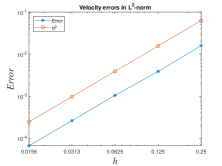
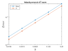
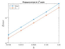
Figure 1: Velocity and pressure errors based on P2-P0 element for Example 7.1.

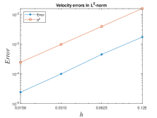
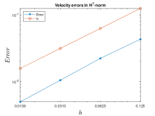
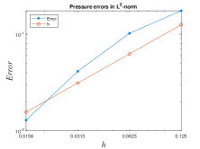
Figure 2: Velocity and pressure errors based on MINI element for Example 7.1.

In order to verify the rate of convergence in both spatial and temporal directions and the uniform convergence in time for nonsmooth data, we consider the following example [10, 30].

Example 7.2.

For initial data ${\bf u}_{0}\in{\bf H}_{0}^{1}$, we take the forcing term $f(x,t)$ such that the solution of the problem to be

$$u_{1}(x,t) =5x^{5/2}(x-1)^{2}y^{3/2}(y-1)(9y-5)\cos{t},$$

$$u_{2}(x,t) =-5x^{3/2}(x-1)(9x-5)y^{5/2}(y-1)^{2}\cos{t},$$

$$p(x,t) =2(x-y)\cos{t}.$$

h	$\|u(t_{n})-U^{n}\|_{L^{2}}$	Rate	$\|u(t_{n})-U^{n}\|_{H^{1}}$	Rate	$\|p(t_{n})-P^{n}\|_{L^{2}}$	Rate
1/4	0.00295597		0.05958679		0.07233700
1/8	0.00071240	2.0529	0.02832958	1.0727	0.03383893	1.0960
1/16	0.00019314	1.8830	0.01456592	0.9597	0.01708781	0.9857
1/32	0.00004903	1.9780	0.00726227	1.0041	0.00845973	1.0143
1/64	0.00001294	1.9217	0.00363780	0.9973	0.00423842	0.9971

Table 3: Errors and convergence rates for backward Euler method for Example 7.2 for P2-P0 element

h	$\|u(t_{n})-U^{n}\|_{L^{2}}$	Rate	$\|u(t_{n})-U^{n}\|_{H^{1}}$	Rate	$\|p(t_{n})-P^{n}\|_{L^{2}}$	Rate
1/8	0.00208654		0.05026012		0.20559044
1/16	0.00054627	1.9334	0.02563557	0.9713	0.10681639	0.9446
1/32	0.00014985	1.8660	0.01262894	1.0214	0.05064130	1.0767
1/64	0.00004098	1.8705	0.00614613	1.0390	0.01583420	1.6772

Table 4: Errors and convergence rates for backward Euler method for Example 7.2 for MINI-element

	P2-P0 element		MINI element
$k$	$\|u(t_{n})-U^{n}\|_{L^{2}}$	Rate	$\|u(t_{n})-U^{n}\|_{L^{2}}$	Rate
1/4	0.00755768		0.02197941
1/16	0.00290626	0.6894	0.00802012	0.7272
1/64	0.00070503	1.0217	0.00207538	0.9751
1/256	0.00019182	0.9389	0.00053884	0.9727
1/1024	0.00004856	0.9909	0.00014555	0.9442

Table 5: $L^{2}$-Errors and convergence rates in temporal direction for Example 7.2 for P2-P0 and MINI-elements

In Table 3 and 4, we have shown the errors and the convergence rates for the backward Euler method using P2-P0 and MINI elements, respectively, with $\mu=1,\gamma=0.1,\delta=1$ and final time $T=1$. The numerical results confirm the optimal convergence rates of the velocity error in ${\bf L}^{2}$-norm as in Theorem 6.2. The error graphs are given in Fig 3 and Fig 4. In Table 5, we present the errors and the convergence rate in temporal direction for P2-P0 and MINI-elements, respectively. Here, we take $k=2^{-2i},~{}i=1,2,\dots,5$, $\mu=1,\delta=0.1,\gamma=0.1,h=\mathcal{O}(\sqrt{k})$ and $T=1$. The error graph is given in Fig 5. We observe that the rate of convergence confirms the theoretical findings.

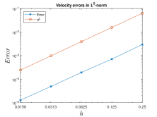
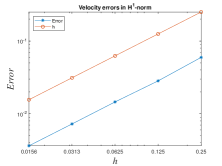
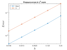
Figure 3: Velocity and pressure errors based on P2-P0 element for Example 7.2.

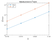
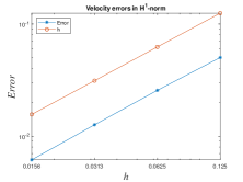
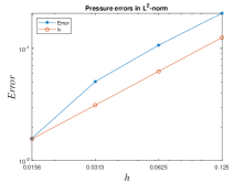
Figure 4: Velocity and pressure errors based on MINI element for Example 7.2.

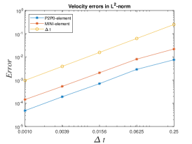
Figure 5: Velocity errors in $L^{2}$- norm with respect to time for Example 7.2.

		P2-P0 element		MINI element
Final time	$h$	$\|u(t_{n})-U^{n}\|_{L^{2}}$	Rate	$\|u(t_{n})-U^{n}\|_{L^{2}}$	Rate
T=10	1/4	0.00475212		0.03323502
	1/8	0.00116079	2.0334	0.00317788	3.3866
	1/16	0.00031742	1.8706	0.00081112	1.9701
	1/32	0.00008496	1.9015	0.00020500	1.9843
	1/64	0.00002272	1.9030	0.00005176	1.9857
T=20	1/4	0.00195842		0.01616627
	1/8	0.00047565	2.0417	0.00156824	3.3657
	1/16	0.00013005	1.8708	0.00040039	1.9697
	1/32	0.00003459	1.9105	0.00010100	1.9870
	1/64	0.00000919	1.9120	0.00002545	1.9885
T=30	1/4	0.00149863		0.00610584
	1/8	0.00036956	2.0197	0.00055113	3.4697
	1/16	0.00010101	1.8713	0.00014395	1.9368
	1/32	0.00002742	1.8810	0.00004044	1.8318
	1/64	0.00000744	1.8824	0.00001135	1.8333
T=40	1/4	0.00446125		0.02641260
	1/8	0.00109409	2.0277	0.00249141	3.4062
	1/16	0.00029908	1.8711	0.00064118	1.9582
	1/32	0.00008028	1.8973	0.00016808	1.9316
	1/64	0.00002153	1.8988	0.00004402	1.9330
T=50	1/4	0.00599158		0.03821832
	1/8	0.00146697	2.0301	0.00363026	3.3961
	1/16	0.00040103	1.8710	0.00093218	1.9614
	1/32	0.00010770	1.8967	0.00024209	1.9451
	1/64	0.00002889	1.8982	0.00006281	1.9465

Table 6: $L^{2}$-Errors and convergence rates for Example 7.2 for P2-P0 and MINI-elements

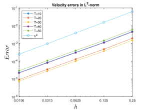
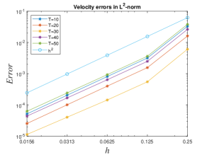
Figure 6: Uniform in time errors for P2-P0 element (left) and MINI element (right) for Example 7.2.

For the example 7.2, the numerical results are shown for final time $T=10,20,30,40$ and $50$ with $\mu=1,\gamma=0.1,\delta=1$, $k=0.1$ and $h=2^{-i},~{}i=2,3,\dots,6$. We represent the errors and the convergence rates for the velocity in ${\bf L}^{2}$-norm for P2-P0 and MINI-elements in Table 6 and Fig 6. The numerical experiments show that for a large time the convergence rates remain same.

		0.1	0.5	1	1.3
	1/10	0.04066058	0.04013758	0.03994627	0.03431507
P2-P0	1/20	0.04060207	0.04007989	0.03988995	0.03426480
element	1/30	0.04059567	0.04007359	0.03988379	0.03425928
	1/40	0.04059327	0.04007121	0.03988147	0.03425720
	1/10	0.04164312	0.03825401	0.03808147	0.03272622
MINI	1/20	0.04310498	0.03967860	0.03949458	0.03393053
element	1/30	0.04334520	0.03991041	0.03972447	0.03412640
	1/40	0.04343595	0.03999863	0.03981201	0.03420103

Table 7: The norm $\sup_{0\leq t_{n}\leq 5}\|U^{n}\|_{L^{2}}$ with nonsmooth data for P2-P0 and MINI elements

		0.1	0.5	1	1.3
	1/10	0.31297840	0.30901528	0.30752906	0.26430325
P2-P0	1/20	0.31034508	0.30641145	0.30500030	0.26201939
element	1/30	0.30987407	0.30594553	0.30454751	0.26161070
	1/40	0.30970478	0.30577810	0.30438480	0.26146391
	1/10	0.32158956	0.29632714	0.29503887	0.25354515
MINI	1/20	0.32860122	0.30352433	0.30217202	0.25959799
element	1/30	0.32979560	0.30474032	0.30337746	0.26062074
	1/40	0.33024171	0.30519856	0.30383212	0.26100694

Table 8: The norm $\sup_{0\leq t_{n}\leq 5}\|U^{n}\|_{H^{1}}$ with nonsmooth data for P2-P0 and MINI elements

		0.1	0.5	1	1.3
	1/10	0.80976358	0.80204569	0.80174532	0.69388452
P2-P0	1/20	0.81411956	0.80642016	0.80616249	0.69778546
element	1/30	0.81499218	0.80729509	0.80704511	0.69856265
	1/40	0.81529345	0.80759726	0.80735004	0.69883114
	1/10	0.86979545	0.85337708	0.85455721	0.73827331
MINI	1/20	0.82750272	0.81637519	0.81639044	0.70638134
element	1/30	0.82289194	0.81236294	0.81225804	0.70293783
	1/40	0.81951684	0.80935013	0.80914669	0.70034738

Table 9: The norm $\sup_{0\leq t_{n}\leq 5}\|P^{n}\|_{L^{2}}$ of with nonsmooth data for P2-P0 and MINI elements

In tables 7 to 9, we have shown the maximal ${\bf L}^{2}$- and ${\bf H}^{1}$-norm of the velocity and maximal $L^{2}$-norm of the pressure among several time steps $k=0.1,0.5,1,1.3$ again for the Example 7.2. The results indicate that the scheme can run well for the values of the time steps going from $k=0.1$ to $k=1.3$, but there is a deterioration of the convergence rate for $k=1$ and $k=1.3$.

8 Conclusion

In this article, optimal error estimates are derived for the backward Euler method employed to the Oldroyd model with non-smooth initial data, that is, ${\bf u}_{0}\in H_{0}^{1}(\Omega)$. For the complete discrete scheme, uniform a priori bounds are shown for the discrete solution. Both optimal and uniform error estimate for the velocity are proved. Uniform estimates are derived under the uniqueness condition. The analysis has been done for the non-smooth initial data and the proofs are more involved in comparison to the smooth case. Our numerical results confirms our theoretical results.

References

[1]Abbaszadeh, M. & Dehghan, M. (2020)
Investigation of the Oldroyd model as a generalized incompressible Navier-Stokes equation via the interpolating stabilized element free Galerkin technique.
Appl. Numer. Math., 150, 274-294.
[2]Akhmatov, M. M. & Oskolkov, A. P. (1989)
On convergent difference schemes for the equations of motion of an Oldroyd fluid.
J. Math. Sci., 47, 2926–2933.
[3]Brezzi, F. & Fortin, M. (1991)
Mixed and Hybrid finite element methods,
Springer Series in Computational Mathematics 15.
New York: Springer-Verlag.
[4]Bercovier, M. & Pironneau, O. (1979)
Error estimates for finite element solution of the Stokes problem in the primitive
variables.
Numer. Math.33, 211–224.
[5]Girault, V. & Raviart, P. A. (1980)
Finite element approximation of the Navier-Stokes equations,
Lecture Notes in Mathematics, 749.
Berlin-New York: Springer-Verlag.
[6]Goswami, D. (2011)
Finite element approximation to the equations of motion arising in Oldroyd viscoelastic model of order one.
Ph.D. Thesis, Department of Mathematics, IIT Bombay.
[7]Goswami, D. & Pani, A. K. (2011)
A priori error estimates for semidiscrete finite element approximations to the
equations of motion arising in Oldroyd fluids of order one.
Int. J. Numer. Anal. Model., 8, 324–352.
[8]Guo, Y. & He, Y. (2016)
An efficient and accurate fully discrete finite element method for unsteady incompressible
Oldroyd fluids with large time step.
Internat. J. Numer. Methods Fluids, 80, 375–394.
[9]Guo, Y. & He, Y., (2018)
On the Euler implicit/explicit iterative scheme for the stationary Oldroyd fluid.
Numer. Meth. Partial Diff. Eqn., 34, 906–937.
[10]He, Y., Huang, P. & Feng, X. (2015)
-Stability of the First Order Fully Discrete Schemes for the Time-Dependent Navier-Stokes Equations.
J. Sci. Comput., 62, 230–264.
[11]He, Y. & Li, K. (1998)
Convergence and stability of finite element nonlinear Galerkin method for the Navier-Stokes equations.
Numer. Math., 79, 77–106.
[12]He, Y., Lin, Y., Shen, S. S. P., Sun, W. & Tait, R. (2003)
Finite element approximation for the viscoelastic fluid motion problem.
J. Comput. Appl. Math., 155, 201–222.
[13]Heywood, J. G. & Rannacher, R. (1982)
Finite element approximation of the nonstationary Navier-Stokes problem: I.
Regularity of solutions and second order error estimates for spatial discretization.
SIAM J. Numer. Anal., 19, 275–311.
[14]Heywood, J. G. & Rannacher, R. (1990)
Finite element approximation of the nonstationary Navier-Stokes problem: I.
Error analysis for second-order time discretization.
SIAM J. Numer. Anal., 27, 353–384.
[15]Liu, C. & Si, Z. (2019)
An incremental pressure correction finite element method for the time-dependent Oldroyd flows.
Appl. Math. Comput., 351, 99-115.
[16]Mohan, M.T. (2020)
Deterministic and stochastic equations of motion arising in Oldroyd fluids of order one: existence, uniqueness, exponential stability and invariant measures.
Stochastic Anal. Appl., 38, 1-61.
[17]Mohan, M.T. (2020)
Well posedness, large deviations and ergodicity of the stochastic 2D Oldroyd model of order one.
Stochastic Processes and their Applications, 130, 4513-4562.
[18]McLean, W. & Thomée, V. (1993)
Numerical solution of an evolution equation with a positive type memory term.
J. Austral. Math. Soc. Ser. B, 35, 23–70.
[19]Oldroyd, J. G. (1956)
Non-Newtonian flow of liquids and solids. Rheology: Theory
and Applications, Vol. I (F. R. Eirich, Ed.).
New York: Academic Press, pp. 653–682.
[20]Pani, A. K. & Sinha, R. K. (1998)
On the backward Euler method for time dependent parabolic integro-differential
equations with nonsmooth initial data.
J. Integral Equations Appl., 10, 219–249.
[21]Pani, A. K. & Sinha, R. K. (1998)
Quadrature based finite element approximations to time dependent parabolic equations
with nonsmooth initial data.
Calcolo, 35, 225–248.
[22]Pani, A. K., Thomée, V. & Wahlbin, L. B. (1992)
Numerical Methods for Hyperbolic and Parabolic Integro-Differential Equations.
J. Integral Equations Appl., 4, 533–584.
[23]Pani, A. K. & Yuan, J. Y. (2005)
Semidiscrete finite element Galerkin approximations to the equations of motion arising in the Oldroyd model.
IMA J. Numer. Anal., 25, 750–782.
[24]Pani, A. K., Yuan, J. Y. & Damazio, P. (2006)
On a linearized backward Euler method for the equations of motion arising in the Oldroyd fluids of order one.
SIAM J. Numer. Anal., 44, 804–825.
[25]Temam, R. (1984)
Navier-Stokes Equations, Theory and Numerical Analysis, Studies in Mathematics and its Application 2, Third Edition.
Amsterdam: North-Holland Publishing Co., pp. xii+526.
[26]Tone, F. & Wirosoetisno, D. (2006)
On the long-time stability of the implicit Euler scheme for the two-dimensional Navier-Stokes equations.
SIAM J. Numer. Anal., 44, 29–40.
[27]Thomée, V. & Zhang, N. Y. (1989)
Error estimates for semidiscrete finite element methods for parabolic
integro-differential equations.
Math. Comp., 53, 121–139.
[28]Wang, K., He, Y. & Shang, Y. (2010)
Fully discrete finite element method for the viscoelastic fluid motion equations.
Disc. Cont. Dyn. Sys. Ser. B, 13, 665–684.
[29]Yang, Y., Lei, Y. & Si, Z. (2020)
Unconditional stability and error estimates of the modified characteristics FEM for the time-dependent viscoelastic Oldroyd flows.
Adv. Appl. Math. Mech., 13, 311–332.
[30]Zhang, T. & Qian, Y. (2018)
Stability analysis of several first order schemes for the Oldroyd model with smooth and nonsmooth initial data.
Numer. Meth. Partial Diff. Eqn., 34, 2180–2216.
[31]Zhang, T., Qian, Y., Jiang, T. & Yuan, J. (2018)
Stability and convergence of the higher projection method for the time-dependent viscoelastic flow problem.
J. Comput. Appl. Math., 318, 1–21.
[32]Zhang, T. & Yuan, J. (2015)
A stabilized characteristic finite element method for the viscoelastic Oldroyd fluid motion problem.
Int. J. Numer. Anal. Model., 12, 617–635.
[33]Zhao, J., Zhang, T. & Qian, Y. (2018)
Stability and convergence of second order time discrete projection method for the linearized Oldroyd model.
Appl. Math. Comput., 316, 342–635.