Latent Space Model for Higher-order Networks and Generalized Tensor Decomposition

Abstract

We introduce a unified framework, formulated as general latent space models, to study complex higher-order network interactions among multiple entities. Our framework covers several popular models in recent network analysis literature, including mixture multi-layer latent space model and hypergraph latent space model. We formulate the relationship between the latent positions and the observed data via a generalized multilinear kernel as the link function. While our model enjoys decent generality, its maximum likelihood parameter estimation is also convenient via a generalized tensor decomposition procedure. We propose a novel algorithm using projected gradient descent on Grassmannians. We also develop original theoretical guarantees for our algorithm. First, we show its linear convergence under mild conditions. Second, we establish finite-sample statistical error rates of latent position estimation, determined by the signal strength, degrees of freedom and the smoothness of link function, for both general and specific latent space models. We demonstrate the effectiveness of our method on synthetic data. We also showcase the merit of our method on two real-world datasets that are conventionally described by different specific models in producing meaningful and interpretable parameter estimations and accurate link prediction.

1 Introduction

Networks (Newman, 2018) capturing the dyadic or pairwise interactions between a set of entities/vertices have been an active research field for more than half a century, leading to millions of publications and technical reports in related disciplines and a wide spectrum of applications. To date, various aspects of networks, e.g. fundamental theories, statistical models, efficient algorithms and so forth, have been well developed through joint contributions from distinct scientific communities – physics, computer science, mathematics, statistics, to name a few. However, the recent decade has witnessed a fast growing demand in processing and analyzing more complex systems where interactions among a set of entities are polyadic or non-linear. These complex networks pose fresh challenges on understanding and exploiting the joint interactions among entities.

The recent boom in data science gives rise to numerous categories of complex networks where relations among entities are far beyond being dyadic. More concretely, we focus on three specific types of complex networks – multi-layer networks (Kivelä et al., 2014), hypergraph networks (Ghoshal et al., 2009) and dynamic/temporal networks (Goldenberg et al., 2010), each of which is an independent sub-field of study and has tremendous applications. Multi-layer networks arise when two vertices can present multiple types of relations, for instance, friendship networks (Dickison et al., 2016; Wang and Li, 2020) on LinkedIn, Instagram and Facebook among the same set of people can differ drastically; trading patterns of different commodities (Jing et al., 2021+; Cai et al., 2021) among the same set of countries are distinct. Other notable examples of multi-layer networks include brain fMRI images (Arroyo et al., 2019; Paul and Chen, 2020a; Tang et al., 2017; Le et al., 2018; Wang et al., 2019), genetic networks and protein-protein interaction networks (Hore et al., 2016; Larremore et al., 2013; Lei et al., 2020; Zhang and Cao, 2017), transportation networks (Cardillo et al., 2013a, b) and etc. Note that the interactions (node $i$, node $j$) in multi-layer networks on each layer are still dyadic. But they can be viewed as polyadic interactions (node $i$, node $j$, layer $l$) if layers are treated as an independent set of entities. Hypergraph networks refer to the complex systems whose vertex interactions are representable by hypergraphs consisting of a set of vertices and a set of hyper-edges. Each hyper-edge can connect multiple (more than $2$) vertices exhibiting a polyadic relationship among these vertices, say (node $i$, node $j$, node $k$). A hypergraph is said to be $m$-uniform if every hyper-edge connects exactly $m$ vertices. Unlike the pairwise interaction of an edge, a hyper-edge captures the higher-order interaction which often carries more insightful information. In (Benson et al., 2016), the authors discover that, by incorporating high-order interactions in the airport network, the spectral clustering algorithm reveals geographic proximity between airports which is unseen if only dyadic relationships are used. Hypergraph networks are typically observed in co-authorship networks (Cai et al., 2021; Ji and Jin, 2016; Newman, 2011), legislator network (Ke et al., 2019; Lee et al., 2017), proton emission networks (Zhen and Wang, 2021), circuit networks (Ghoshdastidar and Dukkipati, 2014) and so on. Lastly, dynamic/temporal networks (Wang et al., 2018) naturally model dynamic systems where interactions between the same set of vertices evolve through time. They resemble multi-layer networks in the sense that layers are now indexed in a meaningful order, such as a discrete time flow. At a fixed time point, the relationship between vertices is still pairwise. Clearly, dynamic networks can be treated as networks of polyadic interactions, say (node $i$, node $j$, time-stamp $t$), if the discrete time flow is viewed as a separate set of entities. Typical examples of dynamic networks include, for instance, the Senate cosponsorship network (Wang et al., 2017), Enron email network (Park et al., 2012; Wang et al., 2013), social interactions between animals (Matias and Miele, 2017) and student friendship network (Chen and Zhang, 2015).

The goal of this paper is to investigate the aforementioned complex and unweighted networks – (mixture) multi-layer networks, hypergraph networks and dynamic/temporal networks in a unified framework. Since these networks all involve joint interactions of multiple entities, we collectively refer to these networks as higher-order networks. We note that, during the preparation of this work, the same concept was also coined by (Bick et al., 2021).

Stochastic block model (SBM) (Holland et al., 1983) is a prevalent approach for modelling the latent group structures of vertices in networks. At the core of SBM is the assumption that vertices belonging to the same group are stochastically equivalent. The group structure of SBM intrinsically impose low-rank constraint on the expected adjacency matrix which naturally popularizes the spectral methods (Rohe et al., 2011; Lei and Rinaldo, 2015; Zhang et al., 2016, 2020b). Undoubtedly, numerous variants of SBM have been proposed to treat higher-order networks. The multi-layer SBM was proposed in Lei et al. (2020); Paul and Chen (2020b); Arroyo et al. (2019) assuming the same group assignments across all layers. A random effect multi-layer SBM was proposed in Paul and Chen (2020a) allowing for heterogeneous group assignments for different layers. More recently, Jing et al. (2021+) introduced a novel mixture multi-layer SBM to simultaneously cluster networks and identify global and local group memberships of vertices. Among these prior works, the low-rankness of adjacency matrix and tensor is the primary ingredient in their methods. Similarly, hypergraph SBM was proposed and theoretically investigated in Ghoshdastidar and Dukkipati (2015, 2017); Chien et al. (2018); Kim et al. (2018); Pal and Zhu (2019); Yuan et al. (2018), where the expected adjacency tensor admits a low-rank decomposition. Meanwhile, Ke et al. (2019) introduced a degree corrected hypergraph SBM to accommodate the degree heterogeneity commonly observed in practice. The authors also proposed a low-rank tensor-based spectral method for community detection. For modelling the group structures in dynamic networks, SBM is also much favored. For instance, Pensky (2019); Pensky and Zhang (2019) studied a dynamic SBM model and a spectral method for community detection. Aside from vertices clustering, another practically relevant problem in dynamic SBM is to detect change points in the sense that, for example, when network structure suddenly shifts. See, e.g., Park et al. (2012); Wang et al. (2013); Wilson et al. (2019); Wang et al. (2017, 2018) for more details. All the aforementioned SBM extensions were designed for treating high-order networks. Without loss of generality, we will collectively refer to them as the high-order SBM.

Higher-order SBM enjoys structural simplicity, motivates diverse new statistical methods and demonstrates effective performances in identifying clusters. However, the stringent model assumptions of SBM may hamper or even jeopardize its effectiveness in handling more general higher-order networks. First of all, SBM enforces transitivity ($i\textrm{ connects to }j,j\textrm{ connects to }k\Rightarrow i\textrm{ connects to }k$ with high probability) via the cluster structure, i.e., nodes in the same cluster tend more likely to connect. However, such strong clustering phenomenon may not be prevalent, especially in high-order networks. Recent advances in analyzing multi-layer networks, such as change point detection in dynamic networks, no longer limit themselves to block model structures (Wang et al., 2018). Secondly, higher-order SBM usually makes the impractical assumption that nodes in the same cluster are stochastically equivalent. As an example, the trading flows of commodities between countries in Section 6; even though China, Germany and USA share similar trading patterns of industrial commodities with other countries, and are identified as being close by a clustering algorithm, they clearly should not be regarded as equivalent in view of the striking technological gaps between these three economies. Finally, due to the linear relations, higher-order SBM usually results into an expected adjacency tensor admitting a low-rank decomposition (Ke et al., 2019; Jing et al., 2021+). Unfortunately, oftentimes, the observed adjacency tensor presents many moderate-magnitude singular values rendering the low-rank presumption questionable.

As argued in Hoff et al. (2002), the transitivity of relations in networks may be better characterized by the proximity between vertices in an unobserved latent space, where each entity/vertex is associated with a vector of characteristics, named latent position, in this space. It is therefore referred to as the latent space model (LSM). Compared with SBM, the learned latent features from LSM (Ma et al., 2020; Levin et al., 2017; Zhang et al., 2020a; MacDonald et al., 2020) is sometimes more useful in downstream tasks such as node visualization, link prediction and community detection. Meanwhile, LSM allows for non-linear relations with a general link or kernel function. In this paper, we propose a unified framework based on LSM to treat higher-order networks – thus the name higher-order latent space model (hLSM). Without loss of generality, we focus on higher-order networks with triadic interactions among vertices. Let ${\cal V}_{1},{\cal V}_{2},{\cal V}_{3}$ be three sets of “vertices” so that a triadic interaction of vertices $i_{1}\in{\cal V}_{1},i_{2}\in{\cal V}_{2},i_{3}\in{\cal V}_{3}$ is notationally regarded as a tuple $(i_{1},i_{2},i_{3})$. We emphasize the abstraction of “vertices” in our framework since they can stand for conceptually different subjects in different contexts. In a hypergraph network, ${\cal V}_{1},{\cal V}_{2},{\cal V}_{3}$ are the same set of vertices and the tuple $(i_{1},i_{2},i_{3})$ just represents a hyper-edge connecting the three vertices. For a multi-layer or dynamic network, ${\cal V}_{1}$ and ${\cal V}_{2}$ can be the same set of vertices while ${\cal V}_{3}$ is viewed as the index set of layers or time-stamps, respectively. Underlying our hLSM is the major assumption that each vertex $i_{k}\in{\cal V}_{k}$, for $k=1,2,3$, is associated with a latent position in a low-dimensional space ${\cal X}_{k}$. Conditioning on the latent positions, hLSM assumes that three vertices positioned $u_{i_{1}}^{\ast},v_{i_{2}}^{\ast},w_{i_{3}}^{\ast}$ would form triadic interaction $(i_{1},i_{2},i_{3})$, independently of others, with probability $\rho(u_{i_{1}}^{\ast},v_{i_{2}}^{\ast},w_{i_{3}}^{\ast})$. Here, $\rho(\cdot):{\cal X}_{1}\times{\cal X}_{2}\times{\cal X}_{3}\mapsto[0,1]$ is called the kernel function of hLSM. The latent positions are treated as fixed points for all vertices whereas we note that our framework can be easily generalized to the case of random latent positions (Athreya et al., 2017). The central task in hLSM is to estimate the latent positions. This inevitably relies on the identifiability of latent positions and the regularity conditions of the kernel function, which shall be unfolded with more details in Section 2. At last, we remark that many aforementioned higher-order SBM’s are special cases of hLSM. By choosing a linear kernel, hSLM reduces to the multi-layer random dot product graph of Levin et al. (2017). With a logistic link and shared latent positions, hLSM reproduces the multi-layer LSM of Zhang et al. (2020a). The hypergraph embedding model proposed in Zhen and Wang (2021) is a special case of hLSM with a joint inner product of latent positions and a transformed logistic link. A special case of hypergraphon is studied in Balasubramanian (2021).

We then investigate a unified framework for estimating the latent positions via generalized low-rank tensor decomposition. At the core of our framework is the assumption that the kernel $\rho$ is a generalized multilinear function in the sense that $\rho(u_{i_{1}}^{\ast},v_{i_{2}}^{\ast},w_{i_{3}}^{\ast})=g(\langle\mathbf{C}^{\ast},u_{i_{1}}^{\ast}\otimes v_{i_{2}}^{\ast}\otimes w_{i_{3}}^{\ast}\rangle)$, where $g(\cdot)$ is a known link function and $\mathbf{C}^{\ast}$ is an unknown interaction tensor. Under the independent-edge assumption, the adjacency tensor $[\mathbf{A}]_{i_{1},i_{2},i_{3}}\stackrel{{\scriptstyle{\rm ind.}}}{{\sim}}\textrm{Bernoulli}\big{(}g([\mathbf{\Theta}^{\ast}]_{i_{1},i_{2},i_{3}})\big{)}$ for an unknown low-rank tensor $\mathbf{\Theta}^{\ast}=\mathbf{C}^{\ast}\cdot\llbracket U^{\ast},V^{\ast},W^{\ast}\rrbracket$. Here $\cdot\llbracket,,\rrbracket$ represents multilinear product, see formal definition in the last paragraph of this section. We estimate the latent positions $U^{\ast},V^{\ast},W^{\ast}$ via the maximum likelihood estimator which is formulated as a problem of generalized low-rank tensor decomposition. Unfortunately, the objective function is highly non-convex and can be solved only locally. Due to the orthogonality assumptions, the latent positions can be treated as points on Grassmann manifolds. We then propose a projected gradient descent algorithm on the Grassmannians. The algorithm is partially inspired by the tensor completion literature (Xia and Yuan, 2019) where its convergence analysis is missing. Here, we investigate this algorithm in a more generalized tensor decomposition framework to treat binary observations. Under mild conditions on the link function, we prove that, even with a constant stepsize, the algorithm converges linearly to a locally optimal solution. This is, to our best knowledge, the first rigorous proof of the fast convergence of the gradient descent algorithm on Grassmannians. Moreover, we also characterize the statistical error of the final estimates of latent positions for general high-order LSM’s. The error rate, determined by the signal strength of interaction tensor and the smoothness of the link function, is optimal in terms of the degrees of freedom. These results are applicable to a novel mixture multi-layer latent space model (MMLSM) and the hypergraph latent space model (hyper-LSM) since they are special cases under our general framework. In particular, our framework is capable of detecting heterogeneous latent positions in multi-layer networks and cluster the layers of networks which might admit similar latent positions. Finally, we also apply our method to a simple dynamic latent space model for change point detection.

Our main contributions can be summarized as follows. First, we introduce a general latent space model, called hLSM in short, to characterize polyadic interactions in higher-order networks, where the participating entities can be real actors in networks or virtual “vertices”. Second, in order to treat heterogeneous multi-layer networks, we propose a novel mixture multi-layer LSM. Unlike the existing literature on multi-layer LSM, our model allows distinct latent positions across layers, prevalent in many real-world applications. Other special cases of hLSM, including hypergraph LSM and dynamic LSM, are presented as well. Third, we formulate a general framework to estimate the latent positions by the maximum likelihood estimator, and propose a projected gradient descent algorithm on Grassmannians. We prove that the algorithm converges linearly if initialized well, and establish the statistical error of final estimates for both general and specific hLSM’s. Finally, the effectiveness of our algorithm is validated on comprehensive simulations and two real-world datasets. We showcase the merits of latent space models in the tasks of node embedding and link prediction.

Notation and Preliminaries on Tensors

Througout the paper, we use $c,c_{0},c_{1},\dots$ and $C,C_{0},C_{1},\dots$ to denote small and large absolute and positive constants, respectively. We write $x\asymp y$ indicating that positive $x$ and $y$ are of same order, i.e., $cy\leq x\leq Cy$. Denote $e_{j}$ the $j$-th canonical base vector whose dimension might vary, depending on the context. For an integer $m$, denote $[m]:=\{1,\cdots,m\}$. Let $\mathbb{O}_{n,p}=\{X\in\mathbb{R}^{n\times p}:X^{T}X=I_{p\times p}\}$ be the collection of all column-orthonormal $n\times p$ matrices. We use uppercase fonts, e.g., $U,W$, to denote matrices and bold uppercase fonts, e.g., $\mathbf{A},\mathbf{\Theta}$, for tensors. Denote the $(i,j,k)$-th entry of $\mathbf{A}$ by $[\mathbf{A}]_{i,j,k}$. For any matrix $A$ with ${\rm rank}(A)=r$, let $\sigma_{1}(A)\geq\sigma_{2}(A)\geq\cdots\sigma_{r}(A)>0$ denote its non-zero singular values. Define $\sigma_{\max}(A):=\sigma_{1}(A)$ and $\sigma_{\min}(A):=\sigma_{r}(A)$. Denote $\|A\|$, $\|A\|_{\infty}$ the spectral norm and max norm of the matrix $A$, respectively. We write $\|A\|_{\rm F}$ ($\|\mathbf{A}\|_{\rm F}$) for the Frobenius norm of the matrix $A$ (tensor $\mathbf{A}$). Define $\|A\|_{2,\infty}:=\max_{j}\|e_{j}^{\top}A\|$.

For an $n_{1}\times n_{2}\times n_{3}$ tensor $\mathbf{A}$, its $1$-st matricization (also called unfolding) ${\cal M}_{1}(\mathbf{A})\in\mathbb{R}^{n_{1}\times(n_{2}n_{3})}$ is defined by $[{\cal M}_{1}(\mathbf{A})]_{i_{1},(i_{2}-1)n_{3}+i_{3}}=[\mathbf{A}]_{i_{1},i_{2},i_{3}}$ for $\forall i_{j}\in[n_{j}]$. The $2$-nd and $3$-rd matricization of $\mathbf{A}$ are defined in a similar fashion. The Tucker ranks of $\mathbf{A}$ are defined by ${\rm rank}(\mathbf{A})=\big{(}{\rm rank}({\cal M}_{1}(\mathbf{A})),({\rm rank}({\cal M}_{2}(\mathbf{A})),({\rm rank}({\cal M}_{3}(\mathbf{A}))\big{)}$. Given a matrix $T\in\mathbb{R}^{r_{1}\times n_{1}}$, the multi-linear product, denoted by $\times_{1}$, between $\mathbf{A}$ and $U$ is defined by $[\mathbf{A}\times_{1}T]_{i_{1},i_{2},i_{3}}=\sum_{j=1}^{n_{1}}[\mathbf{A}]_{j,i_{2},i_{3}}[T]_{i_{1},j}$ for $i_{1}\in[r_{1}]$, $i_{2}\in[n_{2}]$ and $i_{3}\in[n_{3}]$. The other multi-linear products $\times_{2}$ and $\times_{3}$ are defined similarly. If $\mathbf{A}$ has Tucker ranks $(r_{1},r_{2},r_{3})$, there exists an $r_{1}\times r_{2}\times r_{3}$ tensor $\mathbf{C}$, $U\in\mathbb{O}_{n_{1},r_{1}}$, $V\in\mathbb{O}_{n_{2},r_{2}}$ and $W\in\mathbb{O}_{n_{3},r_{3}}$ such that

$$\addcontentsline{lla}{section}{\numberline{\string\crtrefnumber{eq:tucker}}{e}q:tucker}\mathbf{A}=\mathbf{C}\cdot\llbracket U,V,W\rrbracket:=\mathbf{C}\times_{1}U\times_{2}V\times_{3}W,$$ (1)

This is often referred to as the Tucker decomposition of $\mathbf{A}$. We use $\overline{\Lambda}(\mathbf{A}):=\max\{\|\mathcal{M}_{k}(\mathbf{A})\|,k=1,2,3\}$ and $\underline{\Lambda}(\mathbf{A}):=\min\{\sigma_{\min}(\mathcal{M}_{k}(\mathbf{A})),k=1,2,3\}$ to denote the largest and smallest singular values of the tensor $\mathbf{A}$.

2 Higher-order Latent Space Model

For ease of exposition, we only present the hLSM for third-order networks, that is, all interactions among “vertices” are triadic. Its extension to higher-order $(\geq 3)$ networks is conceptually straightforward. Without loss of generality, consider that there exist three sets of “vertices” ${\cal V}_{1},{\cal V}_{2}$ and ${\cal V}_{3}$ with size $n_{k}=|{\cal V}_{k}|$. Here “vertices” are abstractions of “actors” in higher-order networks that can stand for even virtual subjects such as the index of layers in multi-layer networks and time-stamps in dynamic networks.

The observed third-order network is denoted by $\bm{\mathcal{G}}=(\bm{\mathcal{V}},\bm{\mathcal{E}})$ with a set of vertices $\bm{\mathcal{V}}=\{{\cal V}_{1},{\cal V}_{2},{\cal V}_{3}\}$ and a set of triadic interactions $\bm{\mathcal{E}}$. A triadic interaction is a tuple $(i_{1},i_{2},i_{3})$ with vertex $i_{k}\in{\cal V}_{k}$. We say the triadic interaction among the vertices $i_{1},i_{2},i_{3}$ occurs if $(i_{1},i_{2},i_{3})\in\bm{\mathcal{E}}$. The occurrences of distinct triadic interactions are assumed independent akin to the independent-edge random hypergraph (Ke et al., 2019). In hLSM, each vertex is associated with a latent position in an unobserved low-dimensional space characterizing inherent natures of the subjects, e.g. the latent factor for the conservative versus liberal political ideology of senators (Chen et al., 2021). For any tuple $(i_{1},i_{2},i_{3})$, let $u_{i_{1}}^{\ast}\in\mathbb{R}^{r_{1}},v_{i_{2}}^{\ast}\in\mathbb{R}^{r_{2}}$ and $w_{i_{3}}^{\ast}\in\mathbb{R}^{r_{3}}$ be the latent positions of these vertices. Here $r_{k}$ denotes the dimension of the latent space and it usually does not grow as the network size increases, for instance, the political ideology of a senator can be described by a $2$-dim vector – conservatism versus liberalism. Nevertheless, our framework still applies to the cases where $r_{k}$ grows with the network size.

We introduce a kernel function $\rho(\cdot):\mathbb{R}^{r_{1}}\times\mathbb{R}^{r_{2}}\times\mathbb{R}^{r_{3}}\mapsto[0,1]$ such that the triadic interaction $(i_{1},i_{2},i_{3})$ is generated with probability $\rho(u_{i_{1}}^{\ast},v_{i_{2}}^{\ast},w_{i_{3}}^{\ast})$. Fixing the kernel function, the connection probability is determined solely by the latent positions. Denote $\mathbf{A}\in\{0,1\}^{n_{1}\times n_{2}\times n_{3}}$ the binary adjacency tensor of $\bm{\mathcal{G}}$ whose entries are $[\mathbf{A}]_{i_{1},i_{2},i_{3}}={\bf 1}\big{(}(i_{1},i_{2},i_{3})\in\bm{\mathcal{E}}\big{)}$. Under hLSM, we have

$$\addcontentsline{lla}{section}{\numberline{\string\crtrefnumber{eq:bA-def}}{e}q:bA-def}[\mathbf{A}]_{i_{1},i_{2},i_{3}}\stackrel{{\scriptstyle{\rm ind.}}}{{\sim}}\textrm{ Bernoulli}\big{(}\rho(u_{i_{1}}^{\ast},v_{i_{2}}^{\ast},w_{i_{3}}^{\ast})\big{)},\quad\forall i_{k}\in{\cal V}_{k}$$ (2)

Denote $U^{\star}=[u_{1}^{\star},\cdots,u_{n_{1}}^{\ast}]^{\top}\in\mathbb{R}^{n_{1}\times r_{1}}$ (also $V^{\star},W^{\star}$ resp.) the collection of all latent positions of ${\cal V}_{1}$ (also ${\cal V}_{2},{\cal V}_{3}$, resp.). By observing the adjacency tensor $\mathbf{A}$ obeying eq. (2), our goal is to estimate the latent positions $U^{\ast},V^{\ast}$ and $W^{\ast}$.

The general class of kernel functions is too large to estimate. For simplicity, we assume that $\rho(\cdot)$ is a generalized multi-linear function in the sense that

$$\addcontentsline{lla}{section}{\numberline{\string\crtrefnumber{eq:rho-form}}{e}q:rho-form}\rho(u^{\ast},v^{\ast},w^{\ast})=g\big{(}\langle\mathbf{C}^{\ast},u^{\ast}\otimes v^{\ast}\otimes w^{\ast}\rangle\big{)}$$ (3)

where $\mathbf{C}^{\ast}\in\mathbb{R}^{r_{1}\times r_{2}\times r_{3}}$ is an unknown parameter, called the interaction tensor, to be estimated. Here $\otimes$ denotes tensor product and $\langle\cdot,\cdot\rangle$ is the Euclidean inner product. The function $g(\cdot)$ is a known link function, for instance the logistic function $g(x)=(1+e^{-x})^{-1}$ and the probit function $g(x)=\Phi(x)$ where $\Phi(\cdot)$ is the c.d.f. of standard normal random variable. With eq. (2) and (3), we write the expected adjacency tensor by $\mathbb{E}\mathbf{A}=g\big{(}\mathbf{C}^{\ast}\cdot\llbracket U^{\ast},V^{\ast},W^{\ast}\rrbracket\big{)},$ where we slightly abuse the notation and let $g(\cdot):\mathbb{R}\to\mathbb{R}$ also apply entry-wisely on a tensor. If $g(x)=x$ and the latent positions have cluster structures, the model reduces to a higher-order SBM where the expected adjacency tensor admits a low-rank decomposition. Under hLSM with a general link function, $\mathbb{E}\mathbf{A}$ can be full rank while $g^{-1}(\mathbb{E}\mathbf{A})$ is low-rank. Denote $\mathbf{\Theta}^{\ast}=\mathbf{C}^{\ast}\cdot\llbracket U^{\ast},V^{\ast},W^{\ast}\rrbracket$ and then

$$\addcontentsline{lla}{section}{\numberline{\string\crtrefnumber{eq:hLSM}}{e}q:hLSM}[\mathbf{A}]_{i_{1},i_{2},i_{3}}\stackrel{{\scriptstyle{\rm ind.}}}{{\sim}}\textrm{ Bernoulli}([g(\mathbf{\Theta}^{\ast})]_{i_{1},i_{2},i_{3}}),\quad\forall i_{k}\in{\cal V}_{k}.$$ (4)

Note that the independence of entries might hold only for a subset of all entries, e.g., the off-diagonal entries for undirected graphs. Clearly, $\mathbf{\Theta}^{\ast}$ can be uniquely determined by $\mathbb{E}\mathbf{A}$ if the function $g(\cdot)$ is monotonic. However, the latent positions are un-identifiable even with a given $\mathbf{\Theta}^{\ast}$. Without loss of generality, we assume orthonormal latent positions so that $n_{1}^{-1}U^{\ast\top}U^{\ast},n_{2}^{-1}V^{\ast\top}V^{\ast}$ and $n_{3}^{-1}W^{\ast\top}W^{\ast}$ are all identity matrices. We remark that the latent positions sometimes can possess additional structural properties, among which the incoherence is the most prevailing (Jing et al., 2021+; Ke et al., 2019; Han et al., 2020; Cai et al., 2021). The incoherence constant of latent position $U^{\ast}$ is defined by

$$\addcontentsline{lla}{section}{\numberline{\string\crtrefnumber{eq:incoh}}{e}q:incoh}\textsf{Incoh}(U^{\ast}):=n_{1}^{1/2}\|U^{\ast}\|_{\rm F}^{-1}\cdot\max_{1\leq j\leq n_{1}}\|e_{j}^{\top}U^{\ast}\|$$ (5)

Basically, if $\textsf{Incoh}(U^{\ast})$ is upped bounded by a constant, it implies that the majority rows of $U^{\ast}$ have comparable and small magnitudes. It also means that the information $\mathbf{\Theta}^{\ast}$ carries is fairly spread over all its entries.

For ease of references, we refer to hLSM($\mathbf{C}^{\ast},U^{\ast},V^{\ast},W^{\ast},g(\cdot)$) as the higher-order LSM with parameters $\mathbf{C}^{\ast}\cdot\llbracket U^{\ast},V^{\ast},W^{\ast}\rrbracket$ and link function $g(\cdot)$. We now illuminate specific examples of hLSM for mixture multi-layer networks, hypergraph networks and dynamic networks.

2.1 Mixture Multi-layer Latent Space Model

A multi-layer network often consists of multiple networks on the same set of vertices. Denote by $\bm{\mathcal{G}}=({\cal V},\cup_{l=1}^{L}{\cal E}_{l})$ a multi-layer network that is composed of $L$ layers on the set of vertices ${\cal V}$ of size $|{\cal V}|=n$. The $l$-th layer of network, denoted by ${\cal G}_{l}=({\cal V},{\cal E}_{l})$, is an undirected binary graph. This is a special third-order network with ${\cal V}_{1}={\cal V}_{2}={\cal V}$ and ${\cal V}_{3}=[L]$, and $n_{1}=n_{2}=n,n_{3}=L$. Then, its adjacency tensor $\mathbf{A}\in\{0,1\}^{n\times n\times L}$ with its $l$-th slice $[\mathbf{A}]_{:,:,l}$ being the adjacency matrix of the $l$-th layer.

In Zhang et al. (2020a), the authors introduced a multi-layer LSM assuming the unchanged latent positions of vertices across all layers. However, in practice, similarities between vertices can shift drastically on different layers. For instance, when trading industrial commodities with other countries, China and USA are quite similar; whereas these two countries are in completely different positions when trading natural products with other countries. This suggests that a more reasonable model should allow heterogeneous latent positions across different layers. Towards that end, we propose a novel generative model, called mixture multi-layer latent space model (MMLSM). It can be regarded as a generalization of the mixture multi-layer SBM (Jing et al., 2021+).

Suppose that there exists a mixture of $m$ LSMs and each layer $\mathcal{G}_{l}$ is independently sampled from one of these LSM’s. Now each layer has a latent label indicating which class of LSM it is sampled from. More specifically, for each $j\in[m]$, the $j$-th class LSM is described by the latent positions $U_{j}\in\mathbb{R}^{n\times q_{j}}$ with $n^{-1}U^{\top}_{j}U_{j}$ being identity and by a $q_{j}\times q_{j}$ interaction matrix $C_{j}$. Given a link function $g(\cdot)$, if ${\cal G}_{l}$ is sampled from the $j$-th class LSM, its expected adjacency matrix is simply $g(U_{j}C_{j}U_{j}^{\top})$. For simplicity, we denote

• LSM($U_{j},C_{j},g(\cdot)$) — the $j$-th class LSM with parameter $U_{j}$, $C_{j}$ and link function $g(\cdot)$.

• $s_{l}\in[m]$ — the latent label of $l$-th layer for any $l\in[L]$. Denote $\SS=\{s_{1},\cdots,s_{L}\}$.

• $L_{j}=\#\{l:s_{l}=j,l\in[L]\}$ — the number of layers generated by the $j$-th class LSM.

Throughout this paper, we regard the layer labels $\SS$ as being fixed. Consequently, the observed adjacency tensor obeys

$$[\mathbf{A}]_{i_{1},i_{2},l}\stackrel{{\scriptstyle{\rm ind.}}}{{\sim}}\textrm{Bernoulli}\big{(}g([U_{s_{l}}C_{s_{l}}U_{s_{l}}^{\top}]_{i_{1},i_{2}})\big{)},\quad\forall(i_{1},i_{2},l)\in[n]\times[n]\times[L].$$

We call $U_{j}$ the local latent positions of the $j$-th class LSM. Vertices $i_{1}$ and $i_{2}$ are locally similar in the $j$-th class LSM if the $i_{1}$-th and $i_{2}$-th rows of $U_{j}$ are close. Let $\bar{U}=(U_{1},\cdots,U_{m})\in\mathbb{R}^{n\times\bar{q}}$ be the collection of all local latent positions where $\bar{q}=\sum_{j=1}^{m}q_{j}$. The closeness between the $i_{1}$-th and $i_{2}$-th row of $\bar{U}$ implies the global similarities of vertices $i_{1}$ and $i_{2}$ across all layers. MMSLM can be written in the form of hLSM. Define the $\bar{q}\times\bar{q}\times m$ interaction tensor $\mathbf{C}$ such that its $j$-th slice $[\mathbf{C}]_{:,:,j}$ equals ${\rm diag}(0_{q_{1}},\cdots,0_{q_{j-1}},C_{j},0_{q_{j+1}},\cdots,0_{q_{m}})$, where $0_{q}$ denotes the $q\times q$ all-zero matrix. Denote the $L\times m$ layer-label matrix $W=(e_{s_{1}},\cdots,e_{s_{L}})^{\top}$ with $e_{j}$ being the $j$-th canonical basis vector in $\mathbb{R}^{m}$. Thus we can write $\mathbf{\Theta}^{*}=\mathbf{C}\cdot\llbracket{\bar{U}},{\bar{U}},W\rrbracket$ and $\mathbb{E}\mathbf{A}=g(\mathbf{\Theta}^{\ast})$.

Let $W^{\ast}:=L^{1/2}\cdot W\text{diag}(L_{1}^{-1/2},\cdots,L_{m}^{-1/2})$ be the layer latent position matrix such that $L^{-1}\cdot W^{\ast\top}W^{\ast}=I_{m}$. The latent position $W^{\ast}$ reflects how layer label, as an independent “actor”, affects vertex interactions. But $\bar{U}$ may be rank deficient and thus inappropriate to be treated as global latent positions. Denote $r=\textrm{rank}(\bar{U})$ and $n^{-1/2}\bar{U}^{\ast}$ the top-$r$ left singular vectors of $\bar{U}$ so that $n^{-1}\bar{U}^{\ast\top}\bar{U}^{\ast}$ is the identity matrix. We refer to $\bar{U}^{\ast}$ as the global latent positions of vertices. Therefore, $\mathbf{\Theta}^{\ast}$ can be re-parameterized and written as $\mathbf{\Theta}^{\ast}=\mathbf{C}^{\ast}\cdot\llbracket\bar{U}^{\ast},\bar{U}^{\ast},W^{\ast}\rrbracket$ where the new interaction tensor $\mathbf{C}^{\ast}$ is of size $r\times r\times m$. Clearly, $nL^{1/2}\mathbf{C}^{\ast}$ is attainable by multiplying $\mathbf{C}$ with singular values and right singular vectors of $\bar{U}$ in the 1-st and 2-nd modes, and with $\text{diag}(L_{1}^{1/2},\cdots,L_{m}^{1/2})$ in the 3-rd mode, accordingly. Finally, we write

$$\addcontentsline{lla}{section}{\numberline{\string\crtrefnumber{decom:multilayer}}{d}ecom:multilayer}[\mathbf{A}]_{i_{1},i_{2},l}\stackrel{{\scriptstyle{\rm ind.}}}{{\sim}}\textrm{Bernoulli}\big{(}[g(\mathbf{C}^{\ast}\cdot\llbracket\bar{U}^{\ast},\bar{U}^{\ast},W^{\ast}\rrbracket)]_{i_{1},i_{2},l}\big{)},\quad 1\leq i_{1}\leq i_{2}\leq n,l\in[L]$$ (6)

implying that the MMLSM is an hLSM with parameters $\mathbf{C}^{\ast},\bar{U}^{\ast},W^{\ast}$ and the link function $g(\cdot)$. In MMLSM, we aim to estimate the local latent positions $U_{j}$’s, layer latent positions $W^{\ast}$ and global latent positions $\bar{U}^{\ast}$.

We remark that, although we focus on undirected networks, there is no substantial difficulty to generalize our framework to directed cases, in which the entries of parameter tensor can be written in the form $\mathbf{\Theta}^{*}=\mathbf{C}^{*}\cdot\llbracket\bar{U}^{*},\bar{V}^{*},W^{*}\rrbracket$.

2.2 Hypergraph Latent Space Model

A hypergraph network models higher-order interactions, called hyperedges, among a set of vertices. Without loss of generality, we focus on $3$-uniform hypergraph where each hyperedge connects exactly $3$ vertices. We now propose the hypergraph latent space model (hyper-LSM). Let $\mathcal{G}=({\cal V},{\cal E})$ be a 3-uniform undirected binary hypergraph with ${\cal V}=[n]$ being the set of vertices and ${\cal E}$ being the set of hyperedgs, i.e., $(i_{1},i_{2},i_{3})\in{\cal E}$ if there exists a hyperedge among vertices $i_{1}$, $i_{2}$ and $i_{3}$.

In hyper-LSM, each vertex $i\in{\cal V}$ is associated with an unknown latent position vector $u_{i}^{\ast}\in\mathbb{R}^{r}$. Similarly, the probability of generating hyperedge $(i_{1},i_{2},i_{3})$ only depends solely on the latent positions. Suppose $U^{\ast}=(u_{1}^{\ast},\cdots,u_{n}^{\ast})^{\top}$ satisfying $n^{-1}U^{\ast\top}U^{\ast}=I_{r}$ for identifiability. Let $\mathbf{A}\in\{0,1\}^{n\times n\times n}$ be the adjacency tensor of ${\cal G}$. We assume there exists an unknown interaction $r\times r\times r$ tensor $\mathbf{C}^{\ast}$ and a known link function such that

$$[\mathbf{A}]_{i_{1},i_{2},i_{3}}\stackrel{{\scriptstyle{\rm ind.}}}{{\sim}}\textrm{Bernoulli}\big{(}\big{[}g(\mathbf{C}^{\ast}\cdot\llbracket U^{\ast},U^{\ast},U^{\ast}\rrbracket)\big{]}_{i_{1},i_{2},i_{3}}\big{)},\quad\forall 1\leq i_{1}\leq i_{2}\leq i_{3}\leq n$$

implying that $\mathbb{E}\mathbf{A}=g(\mathbf{\Theta}^{\ast})$ where $\mathbf{\Theta}^{\ast}=\mathbf{C}^{\ast}\cdot\llbracket U^{\ast},U^{\ast},U^{\ast}\rrbracket$. Therefore, the hyper-LSM is an hLSM with parameters $\mathbf{C}^{\ast},U^{\ast}$ and the link function $g(\cdot)$

If $g(x)=x$ and $U^{\ast}\in\{0,1\}^{n\times r}$ is a membership matrix such that $U^{\ast}1_{r}=1_{n}$, the hyper-LSM reduces to the hypergraph stochastic block model (Ghoshdastidar and Dukkipati, 2017; Kim et al., 2018; Chien et al., 2018; Yuan et al., 2018). Moreover, if $U^{\ast}$ is the product of a diagonal matrix and a membership matrix, the hyper-LSM becomes the degree corrected block model (Ke et al., 2019).

2.3 Dynamic Latent Space Model

A dynamic network is a times sequence of networks on the same set of vertices. There exist several approaches to model the temporal transition of network structures in dynamic networks (Xu, 2015; Sewell and Chen, 2015; Sarkar and Moore, 2005; Matias and Miele, 2017). For simplicity, we only consider a simple dynamic network model which was often studied for change point detection in dynamic networks (Bhattacharjee et al., 2018).

Let a dynamic network $\bm{\mathcal{G}}=\{{\cal G}_{t}\}_{t=1}^{T}$ compose of a sequence of $T$ networks on the same set of $n$ vertices ${\cal V}$, where the binary graph ${\cal G}_{t}:=({\cal V},{\cal E}_{t})$ represents the interaction at time $t$. Denote $\mathbf{A}\in\{0,1\}^{n\times n\times T}$ the adjacency tensor of $\bm{\mathcal{G}}$ whose $t$-th slice $[\mathbf{A}]_{:,:,t}$ is the adjacency matrix of ${\cal G}_{t}$. For simplicity, we assume the network structures only change at $m\ll T$ unknown time points $\{t_{j}\}_{j=1}^{m}$, called change points (Bhattacharjee et al., 2018; Wang et al., 2018). Here, $t_{1}=1$ and hence the initial network is always identified as a change point. The main task is to identify the other $m-1$ change points and also recover underlying network structures, e.g., the latent positions. For each $j\in[m]$ and $t\in[t_{j},t_{j+1})$, we assume $\mathcal{G}_{t}$ is generated from the same latent space model with the local latent positions $U_{j}^{\ast}\in\mathbb{R}^{n\times q_{j}}$ and interaction matrix $C_{j}^{\ast}\in\mathbb{R}^{q_{j}\times q_{j}}$. We assume $n^{-1}U_{j}^{\ast\top}U_{j}^{\ast}=I_{q_{j}}$ for identifiability and the network layer at each time point is independently sampled from the others. Denote $\bar{U}=(U_{1}^{\ast},\cdots,U_{m}^{\ast})\in\mathbb{R}^{n\times\bar{q}}$ with $\bar{q}=\sum_{j=1}^{m}q_{j}$, whose rows reflect the global similarity between vertices throughout all the time. One can similarly define the interaction tensor as MMLSM of Section 2.1. Consequently, this simple dynamic LSM can be viewed as a special case of MMLSM in that the network layers between two consecutive time change points are sampled from an identical latent space model.

3 Maximum Likelihood Estimation by Tensor Decomposition

In hLSM, with the observed adjacency tensor generated by model (4), our goal is to estimate the latent positions. In view of the low-rank structure of $\mathbf{\Theta}^{\ast}$, a natural solution is the maximum likelihood estimator (MLE) with low-rank constraint. Let $\ell_{n}(\cdot):\mathbb{R}^{n_{1}\times n_{2}\times n_{3}}\mapsto\mathbb{R}$ be the negative log-likelihood for the distribution in hLSM, depending on the choice of a link function $g(\cdot)$. Given the observed binary adjacency tensor $\mathbf{A}$ and a choice of latent parameters $\mathbf{\Theta}\in\mathbb{R}^{n_{1}\times n_{2}\times n_{3}}$, the corresponding negative log-likelihood is1

$$\addcontentsline{lla}{section}{\numberline{\string\crtrefnumber{eq:lnTheta-def}}{e}q:lnTheta-def}\ell_{n}(\mathbf{\Theta}) =-\sum_{i_{j}\in[n_{j}],j\in[3]}\Big{(}[\mathbf{A}]_{i_{1},i_{2},i_{3}}\log g([\mathbf{\Theta}]_{i_{1},i_{2},i_{3}})+(1-[\mathbf{A}]_{i_{1},i_{2},i_{3}})\log(1-g([\mathbf{\Theta}]_{i_{1},i_{2},i_{3}}]))\Big{)}$$ (7)

Under mild regularity conditions on $g(\cdot)$, e.g. strictly increasing monotonicity, the loss function $\ell_{n}(\mathbf{\Theta})$ is convex in $\mathbf{\Theta}$. More details can be found in Section 4. Based on (7), we formulate the rank-constrained as follows

$$\addcontentsline{lla}{section}{\numberline{\string\crtrefnumber{eq:opt-prob}}{e}q:opt-prob}\min_{\mathbf{\Theta}}\ell_{n}(\mathbf{\Theta})\quad\quad\text{subject to}\quad\text{rank}(\mathbf{\Theta})\leq(r_{1},r_{2},r_{3}),$$ (8)

where ${\rm rank}(\cdot)$ denotes the Tucker ranks of a tensor. While the (unconstrained) objective function in problem (8) is usually convex, the rank-constrained feasible set is non-convex. This rank constraint implies the existence of a low-rank decomposition $\mathbf{\Theta}=\mathbf{C}\cdot\llbracket U,V,W\rrbracket$ with $U\in\mathbb{R}^{n_{1}\times r_{1}},V\in\mathbb{R}^{n_{2}\times r_{2}}$ and $W\in\mathbb{R}^{n_{3}\times r_{3}}$. Thus the problem (8) is essentially boiled down to a generalized low-rank tensor decomposition which has been intensively investigated in the literature, e.g. the penalized jointly gradient descent in Han et al. (2020), the Riemannian gradient descent in Cai et al. (2021), the alternating minimization in Wang and Li (2020) and so on. These prior works all take advantage of the specific forms of decomposition of $\mathbf{\Theta}$.

We propose a local algorithm for solving problem (8) by projected gradient descent on Grassmannian. The Grassmannian $\textsf{Gr}(n,r)$ is the collection of all $r$-dimensional subspaces in $\mathbb{R}^{n}$. The Stiefel manifold $\textsf{St}(n,r)=\{U:U^{\top}U=I_{r}\}$ is the set of orthonormal $r$-frames in $\mathbb{R}^{n}$. $\textsf{Gr}(n,r)$ can be obtained by identifying those matrices in $\textsf{St}(n,r)$ whose columns span the same subspace (a quotient manifold), (Edelman et al., 1998). Note that any $U\in\textsf{Gr}(n,r)$ satisfies that $U^{\top}U$ is identity. Thus $\textsf{Gr}(n,r)$ naturally serves as the feasible set for the latent positions in hLSM (4) where $n^{-1/2}U^{\ast}\in\textsf{Gr}(n_{1},r_{1})$. Sometimes $U$ has a bounded incoherence constant so that its row-wise norm is small. To this end, for any $\delta\in(0,1)$, we denote $\textsf{Gr}(n,r,\delta)$ the set of $U\in\textsf{Gr}(n,r)$ such that $\|U\|_{2,\infty}\leq\delta$. Equipped with Grassmannians and by taking advantage of the incoherence property, we reformulate the problem (8) as

$$\addcontentsline{lla}{section}{\numberline{\string\crtrefnumber{eq:opt-prob-ncx}}{e}q:opt-prob-ncx}\min_{\mathbf{C},U,V,W}\ell_{n}\big{(}\mathbf{C}\cdot\llbracket U,V,W\rrbracket\big{)}$$ (9)

$$\text{subject to}\quad U\in\textsf{Gr}(n_{1},r_{1},\delta_{1}),V\in\textsf{Gr}(n_{2},r_{2},\delta_{2}),W\in\textsf{Gr}(n_{3},r_{3},\delta_{3}),$$

where $\delta_{j}\in(0,1)$ are tuning parameters. We show in Section 4 that, under mild conditions and given fixed $U,V,W$, the objective function of (9) is convex with respect to $\mathbf{C}$. Since $\mathbf{C}$ is low-dimensional, optimizing $\mathbf{C}$ is computationally efficient. Thus the major computation challenge lies in the search for optimal $U,V$ and $W$.

The problem (9) is still highly non-convex and solvable only locally where the gradient descent algorithm is often favored. Unfortunately, a naive gradient descent algorithm cannot ensure that the iterated estimations still 1) remain on Grassmannian; and 2) comply with the incoherence condition. The first issue can be resolved by considering the geodesic gradient descent on Grassmannian (Edelman et al., 1998; Xia and Yuan, 2019), but this approach is typically burdensome in computation and greatly complicates theoretical analysis. The second issue is simpler to resolve, for instance, by penalization (Xia and Yuan, 2019) or projection (Ke et al., 2019; Han et al., 2020).

We now propose our approach, based on the projected gradient descent on Grassmannians, for locally optimizing the problem (9). Our algorithm consists of three steps in every iteration.

• Step 1. At $t$-th iteration, given the current estimate $\mathbf{\Theta}^{(t)}=\mathbf{C}^{(t)}\cdot\llbracket U^{(t)},V^{(t)},W^{(t)}\rrbracket$, we calculate the gradients $\nabla_{U}\ell_{n}(\mathbf{\Theta}^{(t)}),\nabla_{V}\ell_{n}(\mathbf{\Theta}^{(t)})$ and $\nabla_{W}\ell_{n}(\mathbf{\Theta}^{(t)})$. With a properly chosen stepsize $\eta>0$, we update the estimate by gradient descent and obtain $\check{U}^{(t)}$ by the left singular vectors of $U^{(t)}-\eta\nabla_{U}\ell_{n}(\mathbf{\Theta}^{(t)})$. This is equivalent to projecting $U^{(t)}-\eta\nabla_{U}\ell_{n}(\mathbf{\Theta}^{(t)})$ onto the Grassmannian and thus $\check{U}^{(t)}\in\textsf{Gr}(n_{1},r_{1})$.

• Step 2. The updated $\check{U}^{(t)}$ from Step 1 may have a large incoherence coefficient. To reinstate incoherence, we impose a regularization that rescales all row $\ell_{2}$-norms higher than $\delta$ down to $\delta$. Formally, for any $U\in\textsf{Gr}(n,r)$, define the regularization operator by

  $$\textsf{Reg}_{\delta}({U}):=D_{U}U,\quad\text{where}\quad D_{U}=\text{diag}\left(\frac{\min\left\{\delta,\|[U]_{1,:}\|\right\}}{\|[U]_{1,:}\|},\cdots,\frac{\min\left\{\delta,\|[U]_{n,:}\|\right\}}{\|[U]_{n,:}\|}\right)$$

  By definition, the output satisfies $\|\textsf{Reg}_{\delta}(U)\|_{2,\infty}\leq\delta$. Then we set $U^{(t+1)}$ to be the left singular vectors of $\textsf{Reg}_{\delta_{1}}(\check{U}^{(t)})$, which provably satisfies $U^{(t+1)}\in\textsf{Gr}(n_{1},r_{1},2\delta_{1})$.

• Update $V^{(t+1)}$ and $W^{(t+1)}$ using the same procedure described in Step 1 and Step 2.

• Step 3. With the updated $U^{(t+1)},V^{(t+1)}$ and $W^{(t+1)}$, we find the core tensor $\mathbf{C}^{(t+1)}$ by solving $\arg\min_{\|\mathbf{C}\|_{\rm F}\leq\xi}\ell_{n}(\mathbf{C}\cdot\llbracket U^{(t+1)},V^{(t+1)},W^{(t+1)}\rrbracket)$ where $\xi>0$ is a tuning parameter. Recall that $\mathbf{C}\in\mathbb{R}^{r_{1}\times r_{2}\times r_{3}}$ is low-dimensional and the objective function is convex (see more details in Section 4) in $\mathbf{C}$, the update $\mathbf{C}^{(t+1)}$ can be efficiently found by Newton-Raphson algorithm.

The implementation details of our algorithm are summarized in Algorithm 1. We note that the gradient can be explicitly computed by

$$\nabla_{U}\ell_{n}(\mathbf{\Theta})={\cal M}_{1}\big{(}\nabla\ell(\mathbf{\Theta})\big{)}(W\otimes V){\cal M}_{1}^{\top}(\mathbf{C}),$$

where recall that $\mathbf{\Theta}=\mathbf{C}\cdot\llbracket U,V,W\rrbracket$.

Algorithm 1 Projected Gradient Descent on Grassmannians

Tuning parameters $\delta_{1},\delta_{2},\delta_{3},\xi>0$; learning rate $\eta>0$; maximum iterations $t_{\max}$; initialization ${U}^{(0)}\in\textsf{Gr}(n_{1},r_{1},\delta_{1})$, ${V}^{(0)}\in\textsf{Gr}(n_{2},r_{2},\delta_{2})$, $W^{(0)}\in\textsf{Gr}(n_{3},r_{3},\delta_{3})$; ${\mathbf{C}}^{(0)}\leftarrow\arg\min_{\|\mathbf{C}\|_{\rm F}\leq\xi}\ell_{n}(\mathbf{C}\cdot\llbracket U^{(0)},V^{(0)},W^{(0)}\rrbracket)$

$\widehat{}\mathbf{\Theta}$, $\widehat{U},\widehat{V},\widehat{W}$

for $t=1,2,\cdots,t_{\max}$ do

     1. ${\mathbf{\Theta}}^{(t-1)}\leftarrow{\mathbf{C}}^{(t-1)}\cdot\llbracket{U}^{(t-1)},{V}^{(t-1)},{W}^{(t-1)}\rrbracket$

     2. (Gradient descent)

$$\check{U}^{(t-1)} \leftarrow{\rm SVD}\big{(}U^{(t-1)}-\nabla_{U}\ell_{n}(\mathbf{\Theta}^{(t-1)})\big{)}$$

$$\check{V}^{(t-1)} \leftarrow{\rm SVD}\big{(}V^{(t-1)}-\nabla_{V}\ell_{n}(\mathbf{\Theta}^{(t-1)})\big{)}$$

$$\check{W}^{(t-1)} \leftarrow{\rm SVD}\big{(}W^{(t-1)}-\nabla_{W}\ell_{n}(\mathbf{\Theta}^{(t-1)})\big{)}$$

     3. (Regularization)

$${U}^{(t)}\leftarrow\text{SVD}\big{(}\textsf{Reg}_{\delta_{1}}(\check{U}^{(t-1)})\big{)};{V}^{(t)}\leftarrow\text{SVD}\big{(}\textsf{Reg}_{\delta_{1}}(\check{V}^{(t-1)})\big{)};{W}^{(t)}\leftarrow\text{SVD}\big{(}\textsf{Reg}_{\delta_{1}}(\check{W}^{(t-1)})\big{)}$$

     4. Compute ${\mathbf{C}}^{(t)}\leftarrow\arg\min_{\|\mathbf{C}\|_{\rm F}\leq\xi}\ell_{n}(\mathbf{C}\cdot\llbracket U^{(t)},V^{(t)},W^{(t)}\rrbracket)$

end for

Set $\widehat{}\mathbf{C}\leftarrow\mathbf{C}^{(t)}$, $\widehat{U}\leftarrow U^{(t)},\widehat{V}\leftarrow V^{(t)},\widehat{W}\leftarrow W^{(t)}$; ${\widehat{}\mathbf{\Theta}}\leftarrow{\widehat{}\mathbf{C}}\cdot\llbracket\widehat{U},\widehat{V},\widehat{W}\rrbracket$

4 Convergence and Estimation Accuracy

We now present the convergence performances of Algorithm 1 and the general statistical error bounds of the final estimates of latent positions. Then we apply these results to several specific hLSM models and elucidate the accuracy of estimated latent positions.

4.1 Regularity conditions on the link and loss functions and properties

The link function $g(\cdot)$ plays a decisive role in the convergence of Algorithm 1. It determines the geometry of loss function $\ell_{n}(\cdot)$. Define

$$g_{+}(x):=\left(\frac{g^{\prime}(x)}{g(x)}\right)^{2}-\frac{g^{\prime\prime}(x)}{g(x)}\quad{\rm and}\quad g_{-}(x):=\left(\frac{g^{\prime}(x)}{1-g(x)}\right)^{2}+\frac{g^{\prime\prime}(x)}{1-g(x)},$$

which are the second order derivative of $\log g(x)$ and $\log(1-g(x))$.

Assumption 1.

Assume that for any small $\alpha>0$, there exist $\gamma_{\alpha},\beta_{\alpha}>0$ depending only on $\alpha$ and $g(\cdot)$ such that

$$\min\left\{\inf_{|x|\leq\alpha}g_{+}(x),\inf_{|x|\leq\alpha}g_{-}(x)\right\}\geq\gamma_{\alpha}$$

$$\max\left\{\sup_{|x|\leq\alpha}g_{+}(x),\sup_{|x|\leq\alpha}g_{-}(x)\right\}\leq\beta_{\alpha}$$

The quantities $\gamma_{\alpha}$ and $\beta_{\alpha}$ are often sensitive to $\alpha$. For instance, if $g(x)=(1+e^{-x/\sigma})^{-1}$ is the logistic link with a global scaling $\sigma>0$, we have $\gamma_{\alpha}=e^{\alpha/\sigma}[\sigma(1+e^{\alpha/\sigma})]^{-2}$ and $\beta_{\alpha}=1/(4\sigma^{2})$; if $g(x)=\Phi(x)$ is the probit link, we have $\gamma_{\alpha}\asymp(\alpha+0.1)(2\pi)^{-1/2}\cdot e^{-\alpha^{2}}$ and $\beta_{\alpha}\geq 0.6$. These examples suggest that $\beta_{\alpha}\gamma_{\alpha}^{-1}$ increases fast as $\alpha$ becomes larger.

We now state our main assumption on the latent positions $U^{\ast},V^{\ast},W^{\ast}$ and the underlying low-rank tensor $\mathbf{\Theta}^{\ast}=\mathbf{C}\cdot\llbracket U^{\ast},V^{\ast},W^{\ast}\rrbracket$ of hLSM (4).

Assumption 2.

Assume that $U^{\ast},V^{\ast},W^{\ast}$ are incoherent with constants upper bounded by $\mu_{0}>0$, i.e. $\textsf{Incoh}(U^{\ast}),\textsf{Incoh}(V^{\ast}),\textsf{Incoh}(W^{\ast})\leq\mu_{0}$. Also, the largest singular value of $\mathbf{C}^{*}$ is upper bounded by ${\overline{\Lambda}}(\mathbf{C}^{*})\leq\alpha\mu_{0}^{-3}(r_{1}r_{2}r_{3})^{-1/2}$.

In hLSM, Assumption 2 implies that $\|U^{\ast}\|_{2,\infty}\leq\mu_{0}r_{1}^{1/2}$, $\|V^{\ast}\|_{2,\infty}\leq\mu_{0}r_{2}^{1/2}$ and $\|W^{\ast}\|_{2,\infty}\leq\mu_{0}r_{3}^{1/2}$. Together with the upper bound of $\overline{\Lambda}(\mathbf{C}^{\ast})$, Assumption 2 implies that $\|\mathbf{\Theta}^{\ast}\|_{\infty}\leq\alpha$. Then, Assumption 1 implies that entry-wisely, $\gamma_{\alpha}\leq g_{+}(\mathbf{\Theta}^{\ast})\leq\beta_{\alpha}$ and $\gamma_{\alpha}\leq g_{-}(\mathbf{\Theta}^{\ast})\leq\beta_{\alpha}$. This is crucial to ensure the strongly convexity and smoothness of the loss function around the truth. The following lemma is straightforwardly implied by Assumption 1, thus we omit its proof.

Lemma 1.

Under Assumption 1, the loss function $\ell_{n}(\cdot)$ is $\gamma_{\alpha}$-strongly convex and $\beta_{\alpha}$-smooth on the set ${\cal K}_{\alpha}:=\{\mathbf{\Theta}\in\mathbb{R}^{n_{1}\times n_{2}\times n_{3}}:\|\mathbf{\Theta}\|_{\infty}\leq\alpha\}$, i.e.,

$$\big{<}\nabla\ell_{n}(\mathbf{\Theta}_{1})-\nabla\ell_{n}(\mathbf{\Theta}_{2}),\mathbf{\Theta}_{1}-\mathbf{\Theta}_{2}\big{>}\geq \gamma_{\alpha}\|\mathbf{\Theta}_{1}-\mathbf{\Theta}_{2}\|_{\rm F}^{2}$$

$$\|\nabla\ell_{n}(\mathbf{\Theta}_{1})-\nabla\ell_{n}(\mathbf{\Theta}_{2})\|_{\rm F}\leq \beta_{\alpha}\|\mathbf{\Theta}_{1}-\mathbf{\Theta}_{2}\|_{\rm F}$$

for any $\mathbf{\Theta}_{1},\mathbf{\Theta}_{2}\in{\cal K}_{\alpha}$.

The next lemma investigates the update of $\mathbf{C}$ in the main iteration of Algorithm 1 and quantifies the convexity of the objective function in $\mathbf{C}$, given properly updated $U,V$ and $W$. We relegate its proof to the appendix (Section 8.1).

Lemma 2.

Suppose Assumption 1 holds. Let $U\in\textsf{Gr}(n_{1},r_{1},\delta_{1}),V\in\textsf{Gr}(n_{2},r_{2},\delta_{2}),W\in\textsf{Gr}(n_{3},r_{3},\delta_{3})$ be fixed with $\delta_{j}\leq\mu_{0}(r_{j}/n_{j})^{1/2}$. If we view $\ell_{n}(\mathbf{C}\cdot\llbracket U,V,W\rrbracket)$ as a function of $\mathbf{C}$, then it is $\gamma_{\alpha}$-strongly convex on the set $\big{\{}\mathbf{C}\in\mathbb{R}^{r_{1}\times r_{2}\times r_{3}}:\|\mathbf{C}\|_{\rm F}\leq\alpha\mu_{0}^{3}(n_{1}n_{2}n_{3}r_{1}^{-1}r_{2}^{-1}r_{3}^{-1})^{1/2}\big{\}}$.

By Lemma 2, with a properly chosen tuning parameter $\xi$, the objective function in the optimization program for updating $\mathbf{C}$ is strongly convex.

4.2 Error bounds of latent position estimates under general hLSM

Let $\{U^{(t)}\}_{t=1}^{t_{\max}},\{V^{(t)}\}_{t=1}^{t_{\max}},\{W^{(t)}\}_{t=1}^{t_{\max}}$ be the iterative updates by Algorithm 1. Notice that, due to the column-normalization of SVD, $U^{(t)}$ (and similarly, $V^{(t)}$ and $W^{(t)}$) estimates $n_{1}^{-1/2}U^{\ast}$ rather than $U^{\ast}$, up to an unknown right-rotation. Therefore, we measure the error of $U^{(t)}$ by the chordal Frobenius-norm distance. Formally, define

$$d_{\textsf{f}}(U^{(t)},n_{1}^{-1/2}U^{\ast}):=\min_{O\in\mathbb{O}_{r}}\|U^{(t)}-n_{1}^{-1/2}U^{\ast}O\|_{\rm F},$$

where $\mathbb{O}_{r}$ is the set of $r\times r$ orthogonal matrices. Define the error measurements for $V^{(t)}$ and $W^{(t)}$ similarly. Then we define the overall error $\textsf{D}_{t}$ at the $t$-th iteration to be

$$\textsf{D}_{t}^{2}:=d_{\textsf{f}}^{2}(U^{(t)},n_{1}^{-1/2}U^{\ast})+d_{\textsf{f}}^{2}(V^{(t)},n_{2}^{-1/2}V^{\ast})+d_{\textsf{f}}^{2}(W^{(t)},n_{3}^{-1/2}W^{\ast})$$

The statistical error of the final estimate $(\widehat{U},\widehat{V},\widehat{W})$ depends on the gradient of the loss function at the truth $\mathbf{\Theta}^{\ast}$. Let $\mathbf{r}=(r_{1},r_{2},r_{3})$ denote the Tucker ranks of $\mathbf{\Theta}^{\ast}$. The stochastic error of the final estimate in hLSM is determined by

$$\textsf{Err}_{\mathbf{r}}:=\sup_{\|\mathbf{X}\|_{\rm F}\leq 1,{\rm rank}(\mathbf{X})=\mathbf{r}}\langle\nabla\ell_{n}(\mathbf{\Theta}^{*})-\mathbb{E}\nabla\ell_{n}(\mathbf{\Theta}^{*}),\mathbf{X}\rangle$$

where recall that $\ell_{n}(\mathbf{\Theta})$ depends on the random $\mathbf{A}$. Under hLSM, we have $\mathbb{E}\nabla\ell_{n}(\mathbf{\Theta}^{\ast})=0$. To see this, first recall that

$$[\nabla\ell_{n}(\mathbf{\Theta}^{\ast})]_{i_{1},i_{2},i_{3}}=\frac{g([\mathbf{\Theta}^{\ast}]_{i_{1},i_{2},i_{3}})-[\mathbf{A}]_{i_{1},i_{2},i_{3}}}{g([\mathbf{\Theta}^{\ast}]_{i_{1},i_{2},i_{3}})\big{(}1-g([\mathbf{\Theta}^{\ast}]_{i_{1},i_{2},i_{3}})\big{)}}\cdot g^{\prime}([\mathbf{\Theta}^{\ast}]_{i_{1},i_{2},i_{3}}).$$

Also recall that $\|\mathbf{\Theta}^{\ast}\|_{\infty}\leq\alpha$ under Assumption 2. Define $\zeta_{\alpha}:=\sup_{|x|\leq\alpha}|g^{\prime}(x)|\big{(}g(x)(1-g(x))\big{)}^{-1}$. Then, the entries of $\nabla\ell_{n}(\mathbf{\Theta}^{\ast})$ are independent centered sub-Gaussian random variables which are uniformly upper bounded by $\zeta_{\alpha}$. The following lemma characterizes the magnitude of the stochastic error $\textsf{Err}_{\mathbf{r}}$, whose proof is deferred to the appendix.

Lemma 3.

Under Assumption 2, there exist an absolute constant $c_{0}>0$ such that with probability at least $1-\exp\big{(}-c_{0}(r_{1}r_{2}r_{3}+n_{1}r_{1}+n_{2}r_{2}+n_{3}r_{3})\big{)}$,

$$\textsf{Err}_{\mathbf{r}}\leq{\zeta_{\alpha}}\cdot\Big{(}{r_{1}r_{2}r_{3}+\sum\nolimits_{k=1}^{3}n_{k}r_{k}}\Big{)}^{1/2}$$

Denote $\kappa_{0}:=\overline{\Lambda}(\mathbf{C}^{*})/\underline{\Lambda}(\mathbf{C}^{*})$ the condition number of $\mathbf{C}^{*}$ and $\bar{r}=\max_{1\leq j\leq 3}r_{j}$. The following theorem shows that, with good initializations and appropriately chosen tuning parameters, Algorithm 1 converges linearly and the error of final outputs only depends on the signal strength $\underline{\Lambda}(\mathbf{C}^{\ast})$ and the stochastic error $\textsf{Err}_{\mathbf{r}}$.

Theorem 1.

Suppose Assumption 1-2 hold in hLSM (4) and $\beta_{\alpha}\leq\gamma_{\alpha}^{2}/(6\kappa_{0}^{2})$. Assume that

1. Initialization error: $\textsf{D}_{0}^{2}\leq c_{1}\kappa_{0}^{-8}/\bar{r}$;

2. Signal-to-noise ratio: $(n_{1}n_{2}n_{3})^{1/2}\cdot\underline{\Lambda}(\mathbf{C}^{\ast})/\textsf{Err}_{\mathbf{r}}\geq C_{1}{\kappa_{0}^{4}\bar{r}}/(\sqrt{c_{1}}\land c_{2})$,

where $c_{1},c_{2},c_{3}\in(0,1)$ and $C_{1}>0$ are constants depending only on $\alpha$ and $c_{2}<c_{3}$. Let the tuning parameters be $\delta_{j}=C_{j}^{\prime}\mu_{0}(r_{j}/n_{j})^{1/2}$ for $1\leq j\leq 3$ and $\xi=C_{4}^{\prime}\alpha\mu_{0}^{3}(n_{1}n_{2}n_{3}r_{1}^{-1}r_{2}^{-1}r_{3}^{-1})^{1/2}$ for some absolute constants $C_{1}^{\prime},C_{2}^{\prime},C_{3}^{\prime},C_{4}^{\prime}>0$. If we choose step size $\eta=\eta_{0}\kappa_{0}^{-4}\underline{\Lambda}^{-2}(\mathbf{C}^{\ast})/\bar{r}$ with $\eta_{0}\in[c_{2},c_{3}]$, we have for all $t=1,\cdots,t_{\max}$ that

$$\textsf{D}_{t}^{2}\leq\Big{(}1-\frac{\eta_{0}\gamma_{\alpha}}{8\kappa_{0}^{6}}\Big{)}^{t}\cdot\textsf{D}_{0}^{2}+\frac{C_{2}\bar{r}\cdot\textsf{Err}_{\mathbf{r}}^{2}}{n_{1}n_{2}n_{3}\cdot\underline{\Lambda}^{2}(\mathbf{C}^{*})},$$

where $C_{2}>0$ depends only on $\alpha$. Then, after at most $t_{\max}=O\big{(}\log(n_{1}n_{2}n_{3}\underline{\Lambda}(\mathbf{C}^{\ast})/(\bar{r}\cdot\textsf{Err}_{\mathbf{r}}))\big{)}$ iterations, we have

$$\textsf{D}_{t_{\max}}^{2}\leq\frac{C_{3}\bar{r}\cdot\textsf{Err}_{\mathbf{r}}^{2}}{n_{1}n_{2}n_{3}\cdot\underline{\Lambda}^{2}(\mathbf{C}^{*})}$$

where $C_{3}>0$ depends only on $\alpha$.

By treating $\eta_{0}$ and $\gamma_{\alpha}$ as constants, the proof of Theorem 1 implies that the joint error of the latent positions estimates by Algorithm 1 contracts as $\textsf{D}_{t+1}^{2}\leq(1-c_{0}/\kappa_{0}^{6})\textsf{D}_{t}^{2}+\textsf{ statistical error}$, where the contraction rate $1-c_{0}\kappa_{0}^{-6}$ is strictly smaller than $1$ with a fixed stepsize. Therefore, Algorithm 1 converges linearly to a locally optimal solution. The initialization condition is also mild. In the case $\kappa_{0},\bar{r}=O(1)$, our theorem only requires $\textsf{D}_{0}\leq c_{4}<1$ for a universal constant $c_{4}.$

By combining Theorem 1 and Lemma 3, we obtain

$$\textsf{D}_{t_{\max}}^{2}\leq\frac{C_{3}\zeta_{\alpha}\cdot\bar{r}(r_{1}r_{2}r_{3}+\sum_{k=1}^{3}n_{k}r_{k})}{n_{1}n_{2}n_{3}\cdot\underline{\Lambda}^{2}(\mathbf{C}^{\ast})}$$

If $\bar{r},\zeta_{\alpha}=O(1)$ and $n_{1}\geq n_{2}\geq n_{3}$, it implies that $\textsf{D}_{t_{\max}}$ converges to zero as long as $n_{2}n_{3}\underline{\Lambda}^{2}(\mathbf{C}^{\ast})\to\infty$. Put it differently, the estimation error of the latent positions diminishes very quickly as the network size grows, which also matches our observations in simulation studies.

4.3 Error bound of latent position estimates for specific hLSMs

We now apply Theorem 1 to the specific examples of hLSM. Here and after, for notational simplicity, we assume the maximum number of iterations $t_{\text{max}}=O\big{(}\log(n_{1}n_{2}n_{3}\underline{\Lambda}(\mathbf{C}^{\ast})/(\bar{r}\cdot\textsf{Err}_{\mathbf{r}}))\big{)}$ under the general LSM model (4). Throughout this section, we assume the initialization condition of Theorem 1 holds.

4.3.1 Application 1: Mixture multilayer latent space model (MMLSM)

Let $\bar{U}=(n^{-1/2}\bar{U}^{\ast})\Sigma_{\bar{U}}R_{\bar{U}}^{\top}$ denote the thin SVD of $\bar{U}$, where the $r\times r$ diagonal matrix $\Sigma_{\bar{U}}$ contains the singular values of $\bar{U}$. To characterize the signal strength of $\mathbf{C}^{\ast}$, define $\bar{\mathbf{C}}=\mathbf{C}\times_{1}R_{\bar{U}}^{\top}\times_{2}R_{\bar{U}}^{\top}$. Simple algebra shows that $\underline{\Lambda}(\mathbf{C}^{*})\geq n^{-1}L^{-1/2}\sigma_{\min}^{2}(\bar{U})\underline{\Lambda}(\bar{\mathbf{C}})\sqrt{\min_{1\leq j\leq L}L_{j}}$. Denote $\kappa_{\bar{U}}$ the condition number of $\bar{U}$. The following corollary is an immediate conclusion from combining Theorem 1 and Lemma 3, whose proof is straightforward and thus omitted.

Corollary 1 (Error bounds of estimating latent positions in MMLSM).

Suppose Assumption 1-2 hold and $\beta_{\alpha}\leq\gamma_{\alpha}^{2}/(6\kappa_{0}^{2})$. Let $\widehat{U}:=U^{(t_{m})}$ be the output of Algorithm 1. Denote the signal strength of $\bar{}\mathbf{C}$ by $c_{\ast}=\underline{\Lambda}(\bar{\mathbf{C}})$. If the network cluster sizes are balanced $\min_{1\leq j\leq m}L_{j}\asymp L/m$, then there exists an absolute constant $c_{0}>0$ such that with probability at least $1-\exp\big{(}-c_{0}(2nr+Lm+mr^{2})\big{)}$

$$\addcontentsline{lla}{section}{\numberline{\string\crtrefnumber{eq:cor_MMLSM_err}}{e}q:cor_{M}MLSM_{e}rr}d_{\textsf{f}}^{2}(\widehat{U},n^{-1/2}\bar{U}^{*})\leq C_{3}\zeta_{\alpha}^{2}\kappa_{\bar{U}}^{4}\frac{(r\vee m)\left(2nr+Lm+mr^{2}\right)}{c_{*}^{2}n^{2}L{m}}$$ (10)

provided that

$$n^{2}L\geq C_{3}\zeta_{\alpha}^{2}\kappa_{\bar{U}}^{4}\left(\frac{r}{{m}}\vee 1\right)\left(2nr+Lm+mr^{2}\right)c_{*}^{-2}$$

where $C_{3}$ is a constant depending only on $\alpha$.

To gain more insight, let us consider a simple setting where $r,m,\zeta_{\alpha},\kappa_{\bar{U}}=O(1)$. The error rate in (10) simplifies to $(n+L)/(c_{\ast}^{2}n^{2}L)$, and we observe an interesting phase transition: (1). when the number of layers $L$ is small compared to $n$, that is $L=O(n)$, the error rate is dominated by the first term $1/(c_{\ast}^{2}nL)$. In this phase, increasing the number of nodes or the number of layers can both improve the estimation of latent positions. (2). when $L\gg n$, the error rate would be bottlenecked by the second term $1/(c_{\ast}^{2}n^{2})$, which does not depend on $L$ anymore. Consequently, increasing the number of layers can no longer improve the estimate of latent positions. This phase transition is also empirically confirmed by our simulation studies, see Section 5. The latter phase seems unexpected since it implies that, beyond certain threshold, increasing the number of layers brings diminishing benefits to the estimation of latent positions. This result, actually, is an outcome due to both the difficulty of the mixture model and the limitation of tensor methods. The mixture nature of MMLSM underlines the importance of estimating the $L\times m$ matrix $W^{\ast}$. However, our tensor method jointly estimates $\bar{U}^{\ast}$ and $W^{\ast}$, and the errors of $\widehat{U}$ and $\widehat{W}$ are thus intertwined. Clearly, when $L\gg n$, estimating $W^{\ast}$ is more difficult than estimating $\bar{U}^{\ast}$. Therefore, in the latter phase, the error rate reflects the difficulty of recovering $W^{\ast}$ rather than estimating $\bar{U}^{\ast}$. This phenomenon can be easily understood from Theorem 1 under general hLSM’s. Indeed, one can expect that for a more general tensor $\mathbf{A}\in\mathbb{R}^{n_{1}\times n_{2}\times n_{3}=L}$, this error bound would become $(n_{1}+n_{2}+n_{3})/(n_{1}n_{2}n_{3})$. Without loss of generality if $n_{1}\gg n_{2},n_{3}$, then the dominating term would be $1/(n_{2}n_{3})$ and increasing $n_{1}$ would only bring diminishing benefits.

We can also recover the network classes $\mathbb{S}$ by applying standard K-means clustering to the rows of $\widehat{W}:=\widehat{W}^{(t_{m})}$ from Algorithm 1. Given an $\widehat{\mathbb{S}}=\{\widehat{s}_{l}\}_{l=1}^{L}$, the estimator of $\mathbb{S}$, we use the average Hamming distance to measure its accuracy:

$$\mathcal{L}(\widehat{\mathbb{S}},\mathbb{S})=\underset{\tau:\text{ a permutation on }[{m}]}{\min}\frac{1}{L}\sum_{l=1}^{L}\mathbbm{1}\left(s_{l}\neq\tau(\widehat{s}_{l})\right)$$

Theorem 2 (Error bounds of network clustering in MMLSM).

Under the conditions of Corollary 1, there exists a global constant $c_{0}>0$ such that with probability at least $1-\exp\big{(}-c_{0}(2nr+Lm+mr^{2})\big{)}$,

$$\mathcal{L}(\widehat{\mathbb{S}},\mathbb{S})\leq C_{3}\zeta_{\alpha}^{2}\kappa_{\bar{U}}^{4}\frac{(r\vee m)\left(2nr+Lm+mr^{2}\right)}{c_{*}^{2}n^{2}L{m}^{2}}$$

provided that

$$n^{2}L\geq C_{3}\zeta_{\alpha}^{2}\kappa_{\bar{U}}^{4}\left(\frac{r}{{m}}\vee 1\right)\left(n\cdot\frac{2r}{{m}}+L+r^{2}\right)c_{*}^{-2}$$

where $C_{3}$ is a constant depending only on $\alpha$.

Corollary 1 and Theorem 2 suggest that, under similar mild signal strength conditions, both the global latent positions and the layer labels can be consistently recovered. Here we have the similar understanding as in Corollary 2 that the accuracy is bottlenecked by the asymptotically smaller one between $n$ and $L$.

Remark 1.

After obtaining the layer labels, one can further estimate the local latent positions for each ${\rm LSM}(U_{j},C_{j})$. Since the layers with equal labels are assumed to be sampled from the same LSM, it is unnecessary to apply tensor methods (the factor corresponding to the third dimension becomes trivially constant). Interested readers may refer to Zhang and Cao (2017); Zhang et al. (2020a) and references therein for more details.

4.3.2 Application 2: Hypergraph latent space model (hyper-LSM)

Similar to Corollary 1, we have the following result.

Corollary 2 (Error bounds of estimating latent position in hyper-LSM).

Suppose Assumption 1-2 hold and $\beta_{\alpha}\leq\gamma_{\alpha}^{2}/(6\kappa_{0}^{2})$. Let $\widehat{U}:=U^{(t_{m})}$ be the output of Algorithm 1. Denote the signal strength of $\mathbf{C}^{\ast}$ by $c_{\ast}=\underline{\Lambda}(\mathbf{C}^{\ast})$. Then there exists some absolute constant $c_{0}>0$ such that with probability at least $1-\exp\big{(}-c_{0}(r^{3}+3nr)\big{)}$,

$$\addcontentsline{lla}{section}{\numberline{\string\crtrefnumber{eq:cor_hLSM_err}}{e}q:cor_{h}LSM_{e}rr}d_{\textsf{f}}(\widehat{U},n^{-1/2}U^{\ast})\leq C_{3}\zeta_{\alpha}^{2}\cdot\frac{3nr+r^{3}}{n^{3}c_{*}^{2}}$$ (11)

provided that

$$n^{2}\geq C_{3}r\left(3+\frac{r^{2}}{n}\right)c_{*}^{-2}$$

with the constant $C_{3}>0$ depending only on $\alpha$.

If $\zeta_{\alpha},r=O(1)$, the error rate (11) simplifies to $1/(n^{2}c_{\ast}^{2})$, where we recall that in an hyper-LSM, by definition $L=n$. This bound diminishes quadratically in $n$. Similarly, the minimal signal strength requirement $c_{\ast}$ also decreases linearly with respect to $n$.

4.3.3 Application 3: Dynamic latent space model (dynamic LSM)

Lastly, we consider the change point detection in dynamic latent space model. With the output $\widehat{W}:=W^{(t_{\text{max}})}$ of Algorithm 1, we perform a row-wise screening to identify the change points $\{t_{m}\}_{m=1}^{M}$. More specifically, we iteratively compare the difference of two consecutive rows of $\widehat{W}$ in $\ell_{2}$ norm, and for all $t\in[T]$, $t+1$ is identified as a change point if and only if

$$\big{\|}[\widehat{W}]_{t,:}-[\widehat{W}]_{t+1,:}\big{\|}_{2}\geq\epsilon$$

for some tuning parameter $\epsilon>0$. Define the $r\times r\times m$ tensor $\bar{\mathbf{C}}$ in the same fashion as in MMLSM, and we can have the following result.

Theorem 3 (Exact detection of change points in dynamic LSM).

Suppose Assumption 1-2 hold and $\beta_{\alpha}\leq\gamma_{\alpha}^{2}/(6\kappa_{0}^{2})$. Denote the signal strength of $\bar{}\mathbf{C}$ by $c_{\ast}=\underline{\Lambda}(\bar{\mathbf{C}})$. If the time intervals between neighboring change points are balanced $\min_{1\leq j\leq m}T_{j}\asymp T/m$, then there exist absolute constants $c_{0},c_{1},c_{2}>0$ such that by choosing $\epsilon\in\big{[}c_{1}(T/m)^{1/2},c_{2}(T/m)^{1/2}\big{]}$, all change points $\{t_{m}\}_{m=1}^{M}$ can be exactly detected with probability at least $1-\exp\big{(}-c_{0}(2nr+Tm+mr^{2})\big{)}$, provided that

$$nT\geq C\kappa_{\bar{U}}^{2}(r\vee m)^{1/2}\left(2nr+Tm+{mr^{2}}\right)^{1/2}\cdot c_{*}^{-1}$$

where $C>0$ is constant depending only on $\alpha$.

If $\kappa_{\bar{U}},r=O(1)$ and $m=O(n)$, by Theorem 3, in order to exactly detect those change points, the minimal signal strength requirement becomes $c_{\ast}^{2}nT^{2}\geq Cm$ for some absolute constant $C>0$.

Our result characterizes the probability of exact change point recovery, which is a natural consequence of accurate latent position estimation, and is different from the noisy recovery error measurement in Wang et al. (2018). Therefore, the signal strength assumption of our Theorem 3 and the counterpart of Wang et al. (2018) are not directly comparable. In fact, our result provide richer information about changes in network evolution that are not limited to sudden changes. For instance, our method is capable of revealing a dynamic network that shows rapid but continuous changes during change periods rather than change points. This pattern is not covered by most change detection literature in network analysis.

5 Simulations on Synthetic Higher-order Networks

In this section, we showcase the performances of Algorithm 1 on synthetic higher-order networks. We first focus on the general higher-order LSM. Then we generate synthetic data from the three application scenarios, namely multi-layer, hypergraph and dynamic networks, discussed in Section 2, and evaluate the numerical performances.

5.1 Simulation 1: general higher-order LSM’s

Without loss of generality, we only consider third-order networks for the general higher-order latent space model (4). The network sizes are fixed at $n_{k}\equiv n=50$ and the dimension of latent space is fixed at $r_{k}\equiv r=3$ for $k=1,2,3$. We generate the low-rank parameter tensor $\mathbf{\Theta}^{\ast}$ as follows. We first generate a truncated standard normal tensor $\widetilde{}\mathbf{\Theta}\in\mathbb{R}^{n\times n\times n}$ with $[\widetilde{}\mathbf{\Theta}]_{ijk}\overset{{\rm i.i.d.}}{\sim}\text{TruncNorm}(0,1;[-3,3]),i,j,k\in[n]$, and then apply higher-order SVD to $10\cdot\widetilde{}\mathbf{\Theta}$ with multilinear ranks $(r,r,r)$, which produces the core tensor $(n_{1}n_{2}n_{3})^{1/2}\mathbf{C}^{*}\in\mathbb{R}^{r\times r\times r}$ and factor matrices $n_{1}^{-1/2}U^{*},n_{2}^{-1/2}V^{*},n_{3}^{-1/2}W^{*}$. The parameter tensor is then set to be $\mathbf{\Theta}^{*}=\mathbf{C}^{*}\cdot\llbracket U^{*},V^{*},W^{*}\rrbracket$. The observed data tensor $\mathbf{A}$ has independent entries sampled from $\text{Bernoulli}(g(\mathbf{\Theta}^{*}/\sigma))$ entry-wisely, where we set the link function $g(\cdot):={\rm logit}(\cdot;\sigma)$ with a global scaling parameter $\sigma\in\{0.1,0.5,1\}$.

The computation of the projected gradient descent updates $U^{(t)},V^{(t)},W^{(t)}$ is fast and memory-efficient. The main computation burden of Algorithm 1 comes from the update of the core tensor $\mathbf{C}^{(t)}$. Computing $\mathbf{C}^{(t)}$ can be recast as essentially estimating a generalized linear model, e.g., logistic/probit regression with logit/probit link function. This step can be computationally demanding when $n_{1}n_{2}n_{3}$ is large. Fortunately, the number of parameters we desire to estimate is only $r_{1}r_{2}r_{3}$, comparatively much smaller than $n_{1}n_{2}n_{3}$. To alleviate the computation costs of this step and accelerate our algorithm, we accelerate by updating $\mathbf{C}^{(t)}$ using a small sub-sample input: $([A]_{{\cal S}_{1},{\cal S}_{2},{\cal S}_{3}};[U^{(t)}]_{{\cal S}_{1},:},[V^{(t)}]_{{\cal S}_{2},:},[W^{(t)}]_{{\cal S}_{3},:}$, where ${\cal S}_{k}\subset[n_{k}]$, $|{\cal S}_{k}|\ll n_{k}$, instead of the original $(A;U^{(t)},V^{(t)},W^{(t)})$, except the last few iterations. This random sampling procedure allows to solve $\mathbf{C}^{(t)}$ via a much smaller scale logistic regression. We regard this method as an accelerated version of Algorithm 1. This accelerated Algorithm 1 can greatly improve speed at little cost of estimation accuracy – Figure 1 and Figure 2 demonstrate that it enjoys almost same convergence and accuracy as the original algorithm. In these simulations, the sampling proportion is $0.1$ and the algorithm runs 5 times faster than the original algorithm.

(a) Algorithm 1

(b) Accelerated version of Algorithm 1

Figure 1: Simulation 1-1 for general hLSM: the convergence of projection error $\|U^{(t)}U^{(t)\top}-n_{1}^{-1}U^{*}U^{*\top}\|_{\rm F}^{2}$ (also for $V,W$ resp.).

(a) Algorithm 1

(b) Accelerated version of Algorithm 1

Figure 2: Simulation 1-2 for general hLSM: the convergence of the logarithm of sum of squares of projection error for $U^{(t)},V^{(t)},W^{(t)}$ under different scales $\sigma\in\{1,0.5,0.1\}$

Figure 1 and Figure 2 present the simulation results. Both figures report that our algorithm converges in around $20$ iterations in terms of the error of latent positions estimates. In Figure 2, a smaller $\sigma$ corresponds to the easier dense network setting, and our algorithm converges even faster. Moreover, the linear pattern at the early stages echos the linear convergence of Algorithm 1 predicted by our theory, see Theorem 1.

5.2 Simulation 2: mixture multi-layer latent space model

We consider the mixture multi-layer latent space model and fix $r=3,m=3$. The global latent position matrix $\bar{U}^{*}\in\mathbb{R}^{n\times r}$ is generated by the $n^{1/2}$ scaling of the left singular vectors of the $n\times r$ random matrix $\widetilde{U}$ with its entries $[\widetilde{U}]_{ij}\overset{{\rm i.i.d.}}{\sim}\mathcal{N}(0.5,1)$. For each $l\in[L]$, we generate the latent network class $s_{l}$ for the $l$-th layer by the uniform multinomial distribution that $\mathbb{P}(s_{l}=j)=m^{-1},j\in[m]$. For each $j\in[m]$, we generate the interaction matrix by $C_{j}=E_{j}E_{j}^{\top}$, where $[E_{j}]_{ik}\overset{{\rm i.i.d.}}{\sim}\text{Uniform}(-1,1)$. The low-rank parameter tensor $\mathbf{\Theta}^{*}=\mathbf{C}^{*}\cdot\llbracket\bar{U}^{*},\bar{U}^{*},W^{*}\rrbracket$, where $\mathbf{C}^{*},W^{*}$ are defined as that in Section 2.1. For each layer $l\in[L]$, set each individual entry of the adjacency tensor by $[\mathbf{A}]_{ijl}\overset{{\rm ind.}}{\sim}\text{Bernoulli}(g([\mathbf{\Theta}^{*}]_{ijl}))$ for $1\leq i<j\leq n$, and $[\mathbf{A}]_{ijl}=0$ for $i=j$. The lower-triangular entries in each slice of $\mathbf{A}$ are set by symmetry.

We run Algorithm 1 on $\mathbf{A}$ and obtain $\widehat{U}$ and $\widehat{W}$, where we initialize $\widehat{U}$ and $\widehat{W}$ for Algorithm 1 by higher-order SVD. We apply K-means clustering to the rows of $\widehat{W}$ and obtain the estimated network classes $\widehat{\mathbb{S}}$ and measure the performance of latent position estimates by $\|\widehat{U}\widehat{U}^{\top}-n^{-1}\bar{U}^{*}\bar{U}^{*\top}\|_{\rm F}$ and that of network clustering by the normalized Hamming error $L^{-1}\mathcal{L}(\mathbb{S},\widehat{\mathbb{S}})$.

Simulation results for various combinations of $n$ and $L$ are shown in Figures 3–5. The two plots in Figure 3 show that the estimation error decreases decently fast as $n$ grows, with large and small $L$, respectively. Comparing the two panels in Figure 4 echoes our intuitive interpretation of our theoretical analysis (Corollary 1) that the method’s accuracy should improve significantly as $L$ grows for $L\ll n$, and such improvement would become diminishing for $L>n$. The same observation goes with the accuracy of the downstream clustering, whose result is presented by Figure 5 and consistent with the prediction of our Theorem 2.

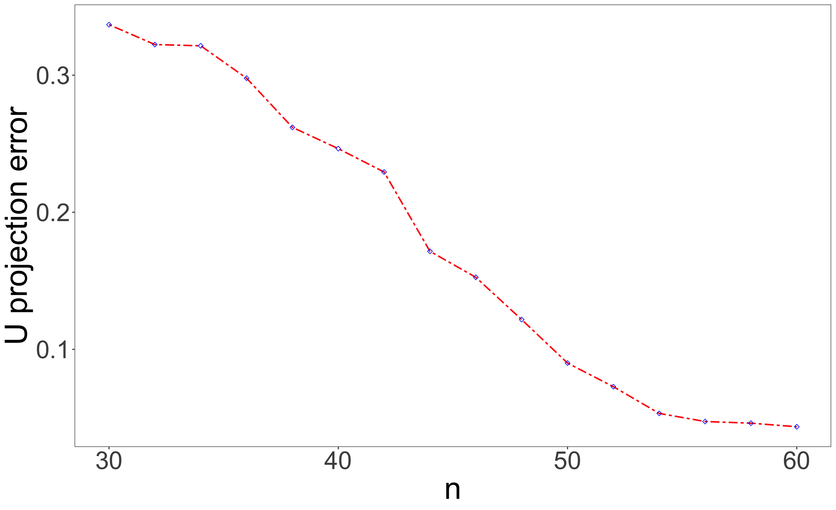
(a) Simulation 2-1 for MMLSM: error of latent position estimates with $n$ varying. Here, $L=150,m=3,r=3$.

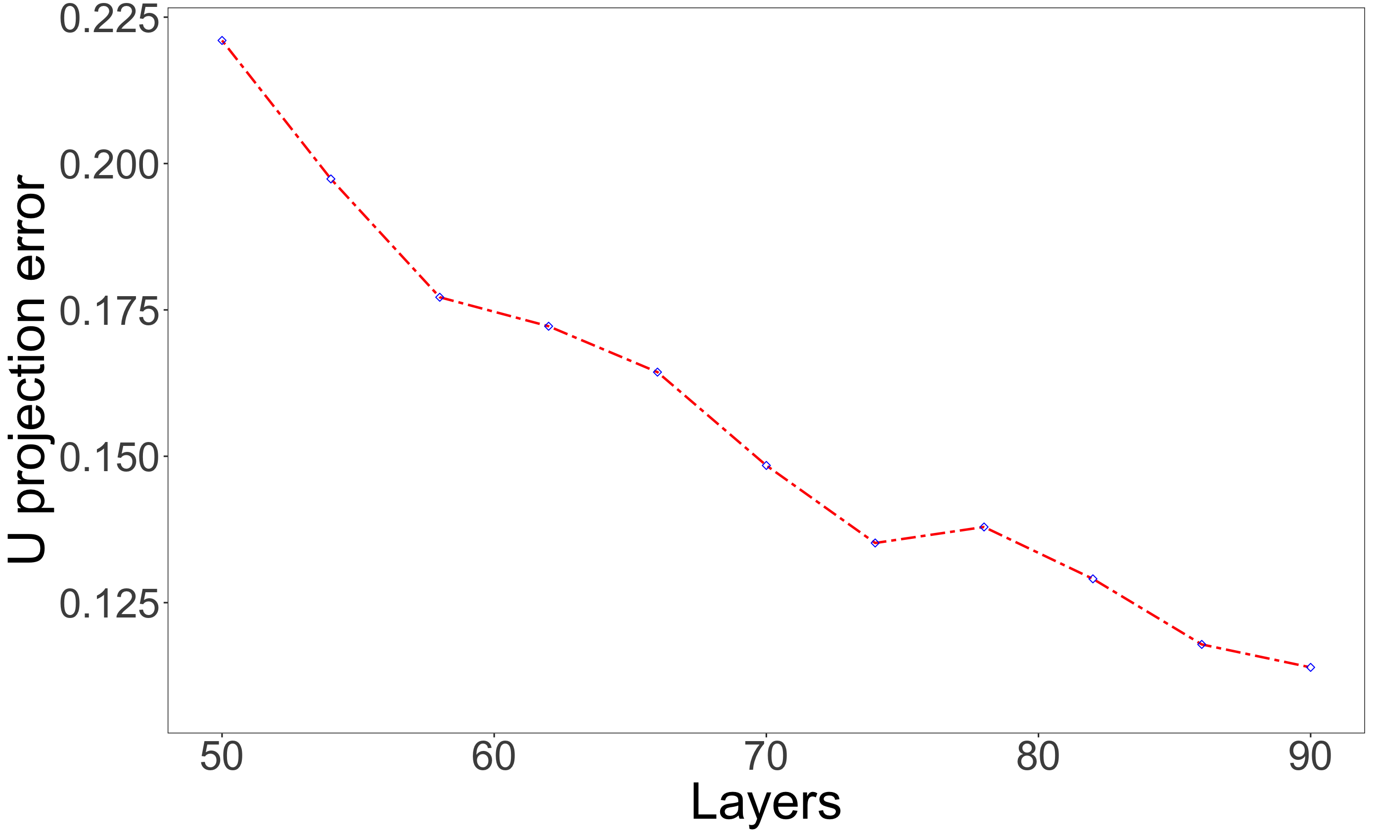
(b) Simulation 2-2 for MMLSM: error of latent position estimates with $n$ varying. Here, $L=20,m=3,r=3$.

Figure 3: Error of latent position estimates with $n$ varying under two scenarios: $n<L$ and $n>L$

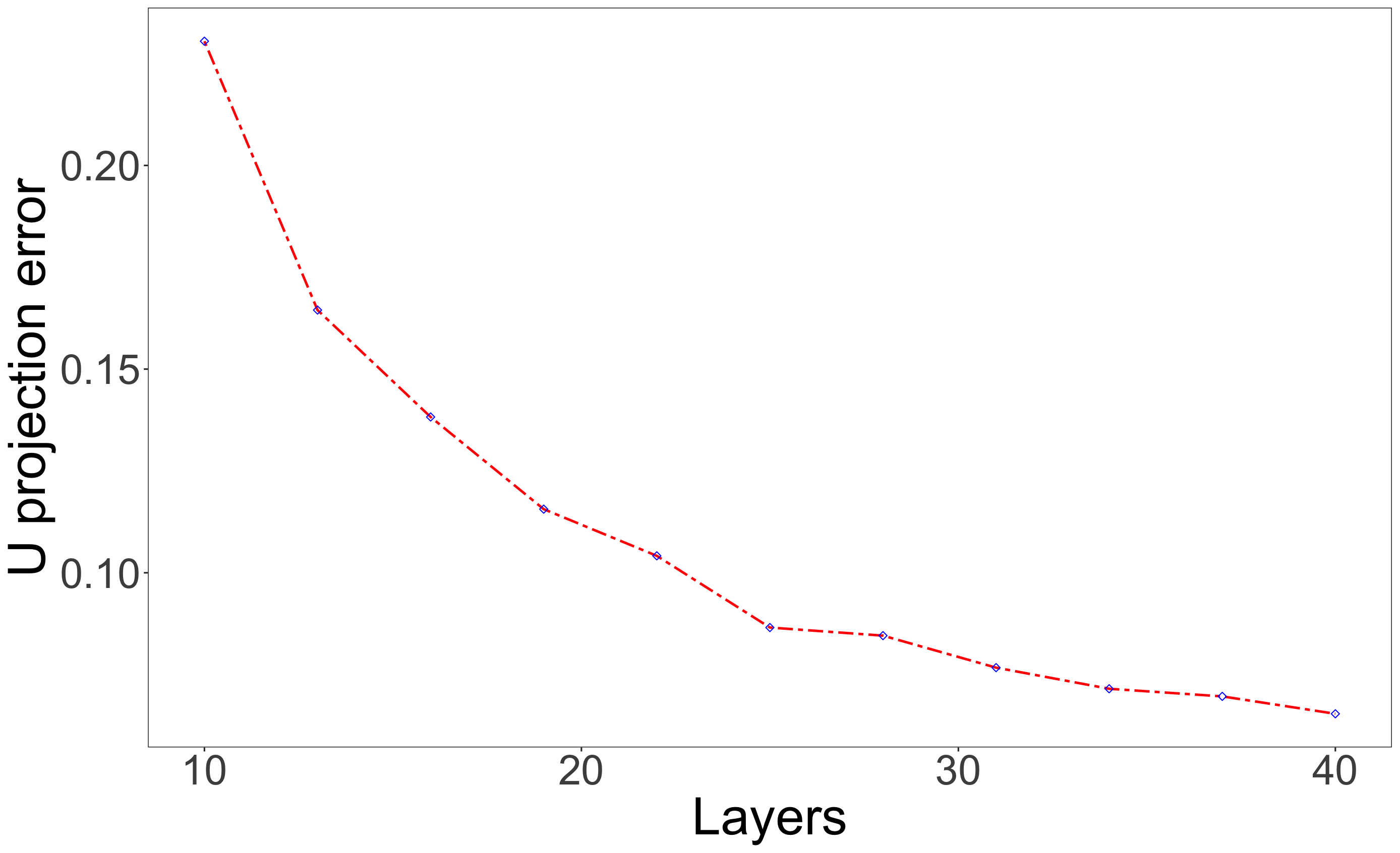
(a) Simulation 2-3 for MMLSM: error of latent position estimates with $L$ varying. Here, $n=100,m=3,r=3$.

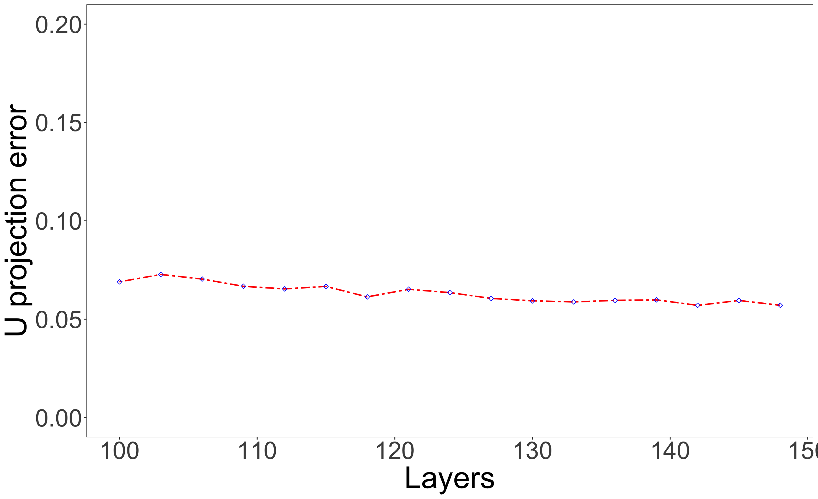
(b) Simulation 2-4 for MMLSM: error of latent position estimates with $L$ varying. Here, $n=50,m=3,r=3$.

Figure 4: Error of latent position estimates with $L$ varying under two scenarios: $L<n$ and $L>n$

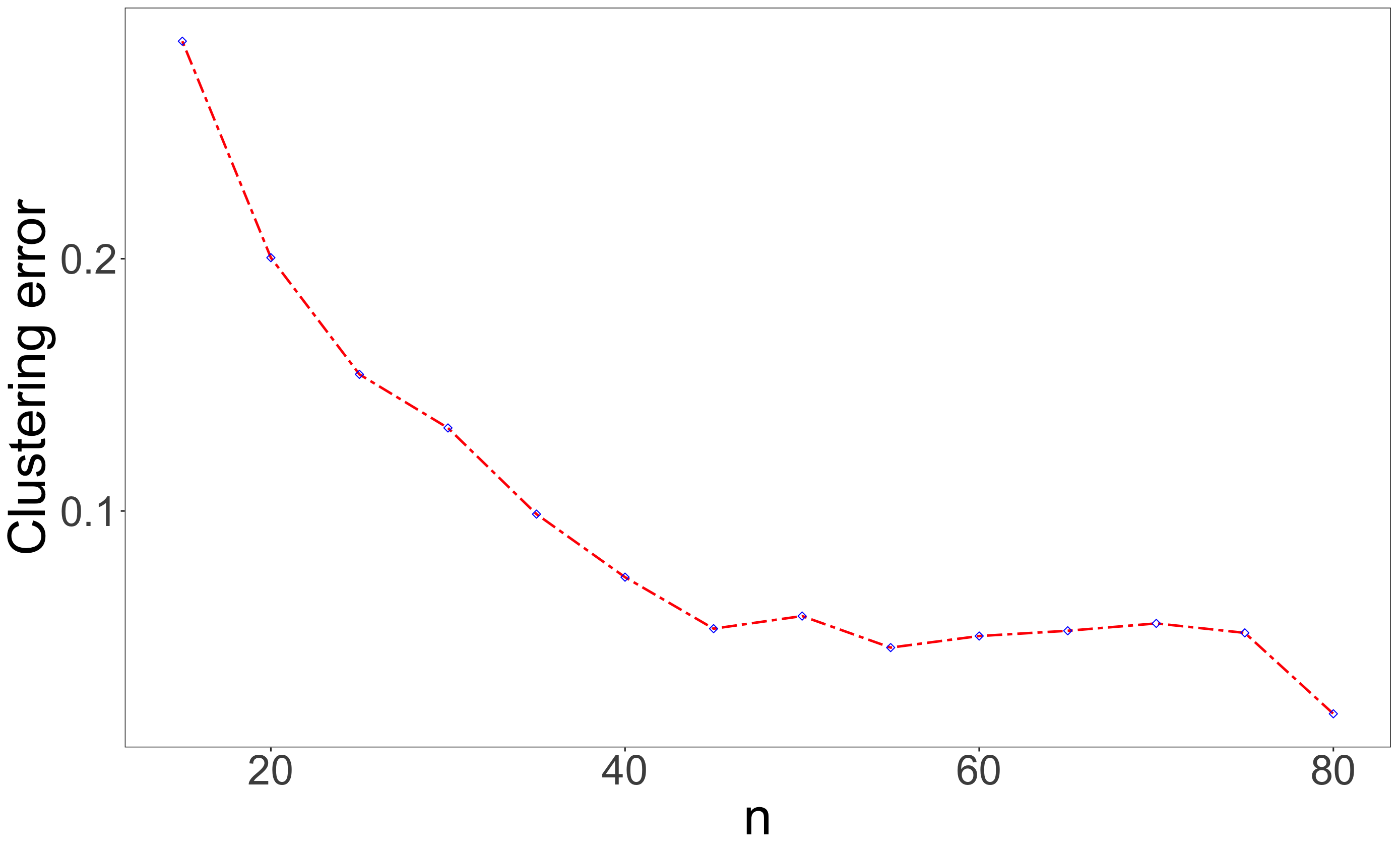
(a) Simulation 2-5 for MMLSM: error of network clustering with $n$ varying. Here, $L=80,m=5,r=3$.

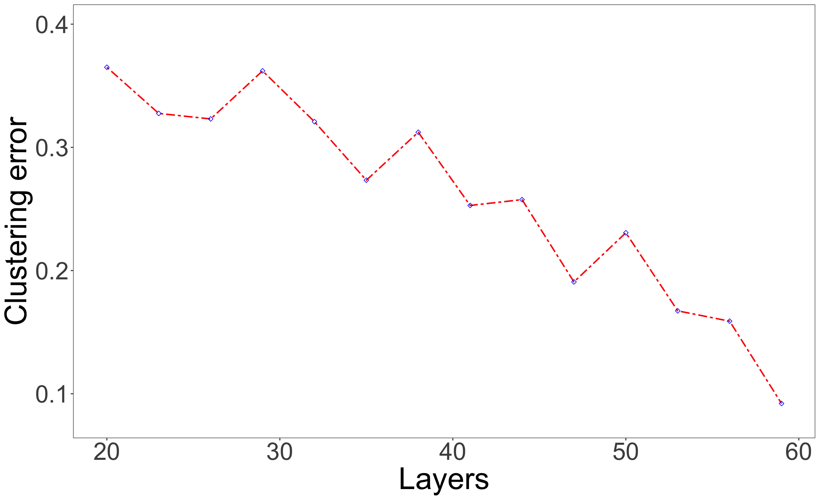
(b) Simulation 2-6 for MMLSM: error of network clustering with $L$ varying. Here, $n=50,m=3,r=3$.

Figure 5: Error of network clustering with $n$ or $L$ varying

5.3 Simulation 3: hypergraph latent space model

We now consider the estimation of latent positions in hyergraphs. Similar to the previous simulations, the dimension of latent space is fixed at $r=3$. Here we generate the latent position matrix $U^{*}$ and interaction tensor $\mathbf{C}^{\ast}$ similarly to Section 5.2. The low-rank parameter tensor in this simulation is $\mathbf{\Theta}^{*}=\mathbf{C}^{*}\cdot\llbracket U^{*},U^{*},U^{*}\rrbracket$. Each entry of the adjacency tensor is sampled by $[\mathbf{A}]_{ijk}\overset{{\rm ind.}}{\sim}\text{Bernoulli}(g([\mathbf{\Theta}^{*}]_{ijk}))$ for $1\leq i<j<k\leq n$ and $A_{ijk}=0$ if $i,j,k$ are not all distinct. The lower-triangular entries are also determined by symmetry, slice-wisely.

Due to symmetry, it suffices to estimate the singular vectors $U$. Using Algorithm 1 again with the higher-order SVD initialized $U^{(0)}$, we obtain an estimation for $\widehat{U}$. We define the error measurement for this setting by $\|\widehat{U}\widehat{U}^{\top}-n^{-1}U^{*}U^{*\top}\|_{\rm F}^{2}$.

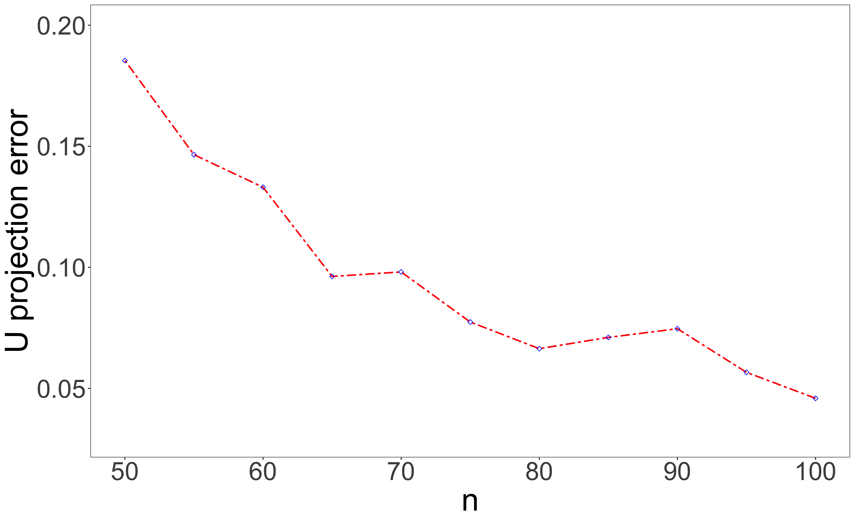
(a) Simulation 3-1 for hyper-LSM: error of latent position estimates with $n$ varying. Here, $r=3$.

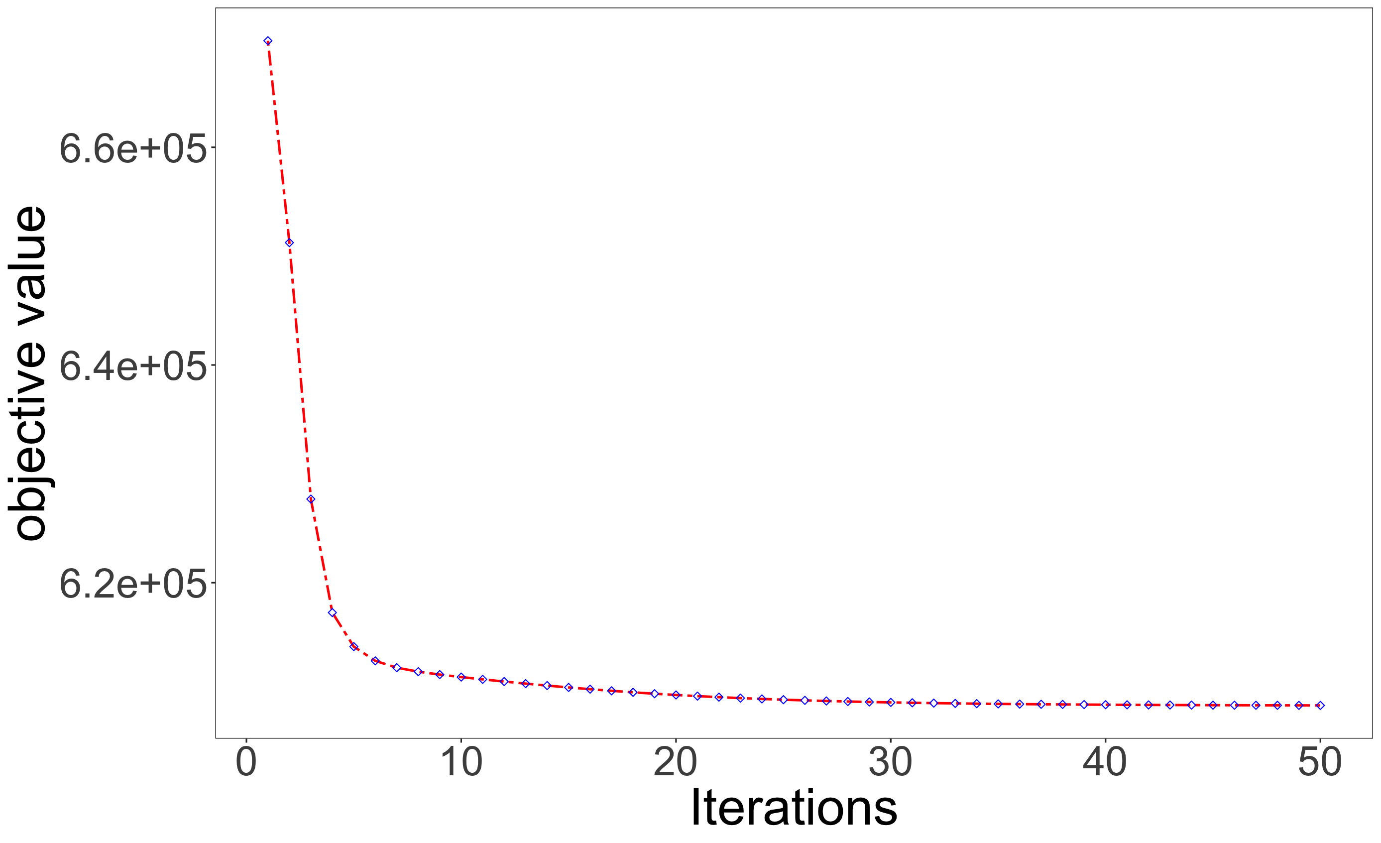
(b) Simulation 3-2 for hyper-LSM: value of objective function with respect to the iterations. Here, $n=100,r=3$.

Figure 6: Error of latent position estimates with $n$ varying; decrease of objective value with respect to iterations

The two panels of Figure 6 present the results on accuracy and convergence. Plot (a) shows that, again, estimation error decreases decently fast in $n$, consistent with our Corollary 2. In plot(b), the objective value shows linear decrement before hitting convergence in just about $5$ iterations. This demonstrates our method’s fast convergence rate and matches our theoretical prediction.

5.4 Simulation 4: dynamic latent space model

In the experiment, we set $n=50$, and, for simplicity, $q_{j}=2$ (the rank of $U_{j}^{*}$ in all time intervals) for all $j\in[m]$ as we are interested in change point detection. We randomly pick $m=4$ change points $\{t_{j}\}_{j=2}^{m}$ uniformly from $\{2,\cdots,T\}$. For each layer corresponding to the time interval $t\in(t_{j},t_{j+1}]$, we generate the latent position matrix $U_{j}$ and the interaction matrix $C_{j}$ similarly to that in Section 5.2. We apply Algorithm 1 with warm initializations attained by HOSVD and focus on the estimated $\widehat{W}$. We run a row-wise screening procedure (see Section 4.3.3) on $\widehat{W}$ to identify change points. We measure the performance by the proportion of repeated experiments that correctly identify both the number of change points and their locations.

	Exact detection rate	Accuracy
T=20	0.50	$0.82\pm 0.24$
T=50	0.85	$0.94\pm 0.14$
T=80	0.96	$0.99\pm 0.07$

Table 1: Simulation 4-1 for dynamic LSM: rate of exact detection and accuracy over $100$ simulations

Table 1 reports the result over 100 simulations. The exact detection rate increases as $T$ grows, which aligns with our Corollary 3.

6 Data examples

In this section, we demonstrate the merits of our methods in node embedding and link predictions on two real-world datasets.

6.1 Trade flow multi-layer network from UN Comtrade

The multi-layer network data are constructed based on the international commodity trade data collected from the UN Comtrade Database (https://comtrade.un.org). The dataset contains annual trade information for countries/regions from different continents in 2019, where, for ease of presentation, we only focus on the top representative $48$ countries/regions ranked by the exports of goods and services in US dollars. Each layer represents a different type of commodities classified into $97$ categories based on the 2-digit HS code (https://www.foreign-trade.com/reference/hscode.htm). For every two nodes $i$ and $j$, we convert the two weighted edges $w_{i\to j},w_{j\to i}\geq 0$ in the original data into one binary directed edge: if $w_{i\to j}>w_{j\to i}$ then we set $A_{i\to j}=1,A_{j\to i}=0$, indicating a trade surplus of $i$ in its trade with $j$, and vice versa. The adjacency tensor $\mathbf{A}$ is defined in the way such that $[\mathbf{A}]_{ijl}=1$ if country $i$ exports to country $j$ in terms of commodity type $l$. We remove empty layers and obtain a binary adjacency tensor $\mathbf{A}$ of size $48\times 48\times 97$.

We apply our Algorithm 1, initialized by HOOI (Zhang and Xia, 2018; Ke et al., 2019), to $\mathbf{A}$ and obtain an estimated $\widehat{W}$. Empirical evidence (the numerical scales of the leading eigenvalues and the plot of $\widehat{W}$ rows projected onto the first two principal components) suggest that $r=5$ and $m=2$ lead to a most interpretable model fit. Then we apply K-means clustering on the rows of $\widehat{W}$ with $m=2$ clusters and report the result in Table 2. It is interesting to observe that bio-related daily products including animal & animal products, vegetable products, over half of foodstuffs fall into cluster $1$, most of which are all products of low durability. On the other hand, most industrial products including main parts of chemicals & allied industries, plastic/rubbers, stone/glass, machinery/electrical, aircraft, spacecraft, optical, photographic, etc., and clocks and watches constitute cluster $2$.

Based on the layers clustering in Table 2, we further investigate the shared trade pattern among different countries/regions. Specifically, we construct a sub-tensor of size $49\times 49\times 20$ from cluster $1$ for bio-related commodities, and a sub-tensor of size $49\times 49\times 15$ from cluster $2$ for industrial commodities. A scientifically interesting question is to compare the latent position representations in these two groups of layers. Toward this end, we apply Algorithm 1 with $r=3$ and $m=1$ on these two sub-tensors. Since the trading flows are directed, the left singular vectors $\widehat{U}$ and right singular vectors $\widehat{V}$ are distinct. It turns out that the latent position of imports $\widehat{V}$ provide clear and interpretable results. We further perform multidimensional scaling (MDS) on the rows of $\widehat{V}_{\textsf{bio}}$ and $\widehat{V}_{\textsf{ind}}$, projecting them into $\mathbb{R}^{2}$ for visualization. In Figure 7 and Figure 8 plot the projected embedding of countries/regions according to their latent positions $\widehat{V}_{\textsf{bio}}$ and $\widehat{V}_{\textsf{ind}}$ after MDS, with nodes being colored by corresponding continents.

The latent positions of countries/regions for the two groups of layers exhibit different patterns. In Figure 7, latent positions for countries/regions in the same continent in general are close to each other, which to some extent reflects geographic proximity relations. We could observe several “clusters” such as European countries in the bottom right and the top middle; Hong Kong SAR, Singapore, South Korea (three out of Four Asian Tigers) and Japan in the bottom middle; Indonesia, Philippines, Thailand and Malaysia (known as Tiger Cub Economies). This is reasonable since for commodities of low durability, regional trade partnerships usually dominate the inter-continental ones. However, it is interesting to notice those outliers. Three large economies China, USA and Canada are relatively close in latent positions even though China is not geographically close to USA and Canada, since they export a large amount of bio-related/daily products to all other countries. Three South America countries (Argentina, Chile and Brazil), two Africa countries (Nigeria and South Africa) and Mexico are embedded closer to the Middle East countries, as these nations import similar products mainly from several largest exporting economies. In Figure 8, the geographical impact, to some extent, is weakened. Germany, originally near United Kingdom, France and Netherlands in Figure 7, is now clustered closer to China and USA, largely due to the fact that they are all big industrial nations with a huge demand of importing industrial raw materials. Denmark, Austria and Sweden (three out of Frugal Four) are mixed with countries/regions from Asia, South America and Africa, indicating that these developed industrial nations are heavily depending on imported industrial products from those developing countries. Australia is relocated nearer to European nations, which can be explained by their similarity of imported goods which outweighs the geographical closeness to Asian nations. Overall, high durability for industrial products means relatively low cost in freight and hence the trade partnerships are less regionally restricted and more related to their resemblance and connection in terms of industrial products.

To further assess the performance of the estimated latent positions, we apply our method to this dataset for the task of link prediction. We adopt the evaluation metric for link prediction in Zhao et al. (2017). Specifically, we set $20\%$ of entries of $\mathbf{A}$ ($10\%$ randomly selected out of non-zero entries and $10\%$ out of zero entries) to be $0$ and construct the test tensor data $\mathbf{A}_{\textsf{test}}$. Then Algorithm 1 is applied to $\mathbf{A}_{\textsf{test}}$ to get the estimated probability tensor $\widehat{\mathbf{P}}=g(\widehat{}\mathbf{\Theta})$. We evaluate the link prediction performance on those randomly deleted entries by AUC, which is defined to be the area under the ROC curve. By 30 simulations, we observe $\text{AUC}=0.910(\pm 0.001)$. The ROC curve with $99.9\%$ confidence interval is displayed in Figure 9.

Commodity cluster 1

01-05 Animal & Animal Products (100%) 06-15 Vegetable Products (100%) 16-18,23-24 Foodstuffs (56%) 26 Mineral Products (33%) 31,36-37 Chemicals & Allied Industries (27%) 41,43 Raw Hides, Skins, Leather & Furs (66%) 45-47 Wood & Wood Products (50%) 50-55,57-58,60 Textiles (64%) 66-67 Footwear / Headgear (50%) 75,78-81 Metals (45%) 86,89 Transportation (50%) 92,93,97 Miscellaneous (37.5%)

Commodity cluster 2

19-22 Foodstuffs (44%) 25,27 Mineral Products (67%) 28-30,32-35,38 Chemicals & Allied Industries (73%) 39-40 Plastics / Rubbers (100%) 42 Raw Hides, Skins, Leather, & Furs (33%) 44,48-49 Wood & Wood Products (50%) 56,59,61-63 Textiles (36%) 64,65 Footwear / Headgear (50%) 68-71 Stone / Glass (100%) 72-74,76,82-83 Metals (55%) 84-85 Machinery / Electrical (100%) 87-88 Transportation (50%) 90-91,94-96,99 Miscellaneous (62.5%)

Table 2: Network clustering results of 97 commodity layers, $\%$ denote the proportion of number of layers in the same category characterized by HS Code

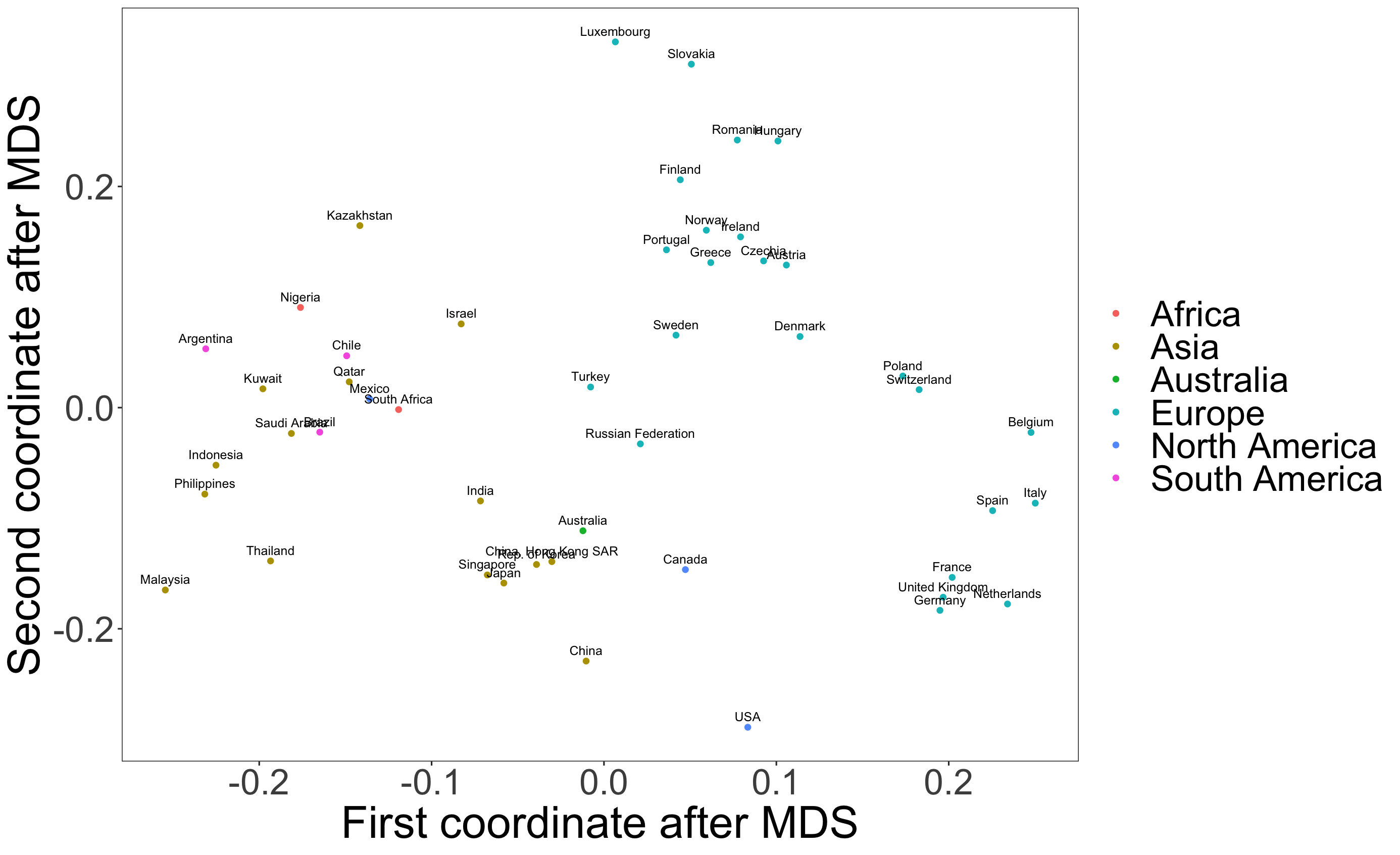
Figure 7: Latent positions of countries/regions for layers of bio-related daily products

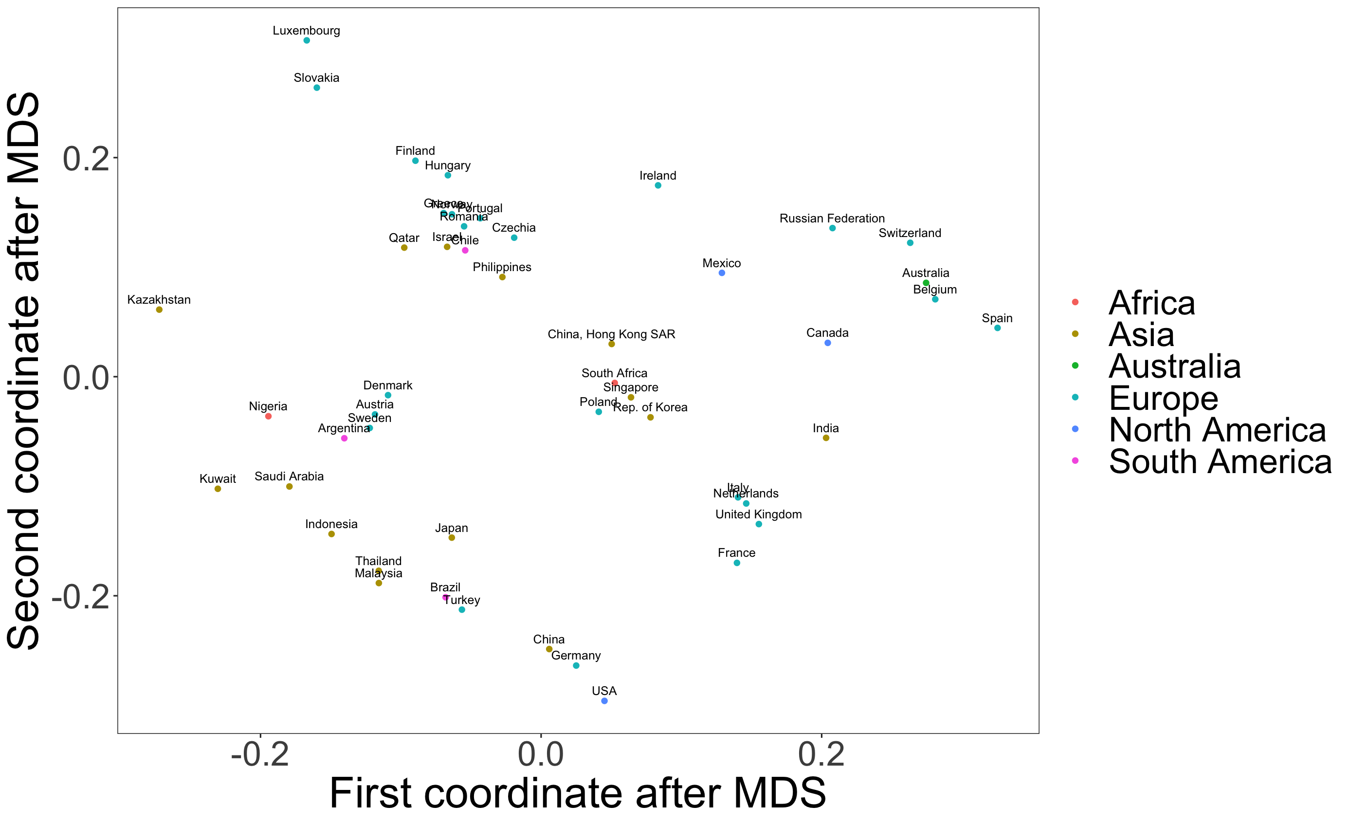
Figure 8: Latent positions of countries/regions for layers of industrial products

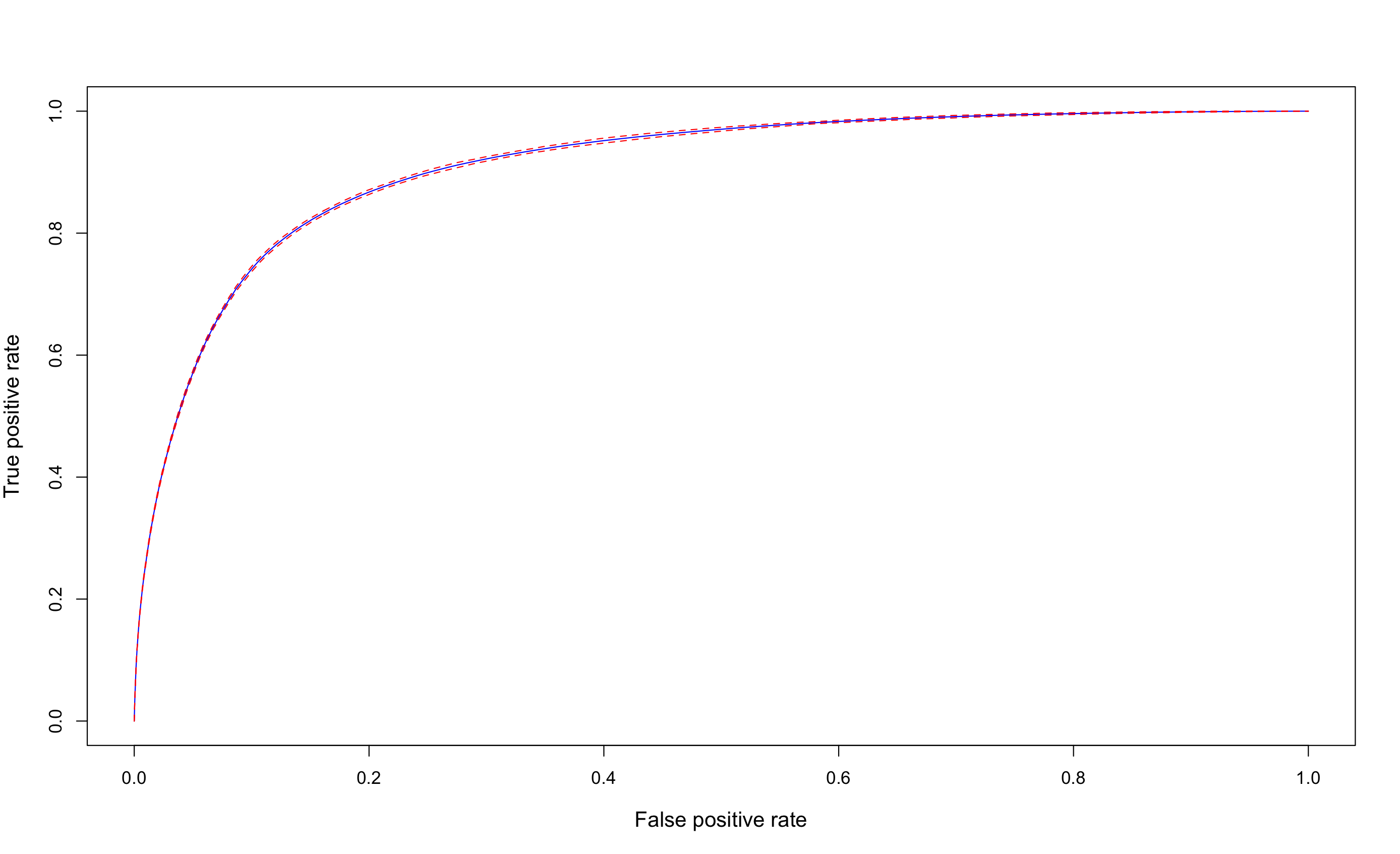
Figure 9: ROC curve for link prediction with $99.9\%$ CI (red dashed line)

6.2 Disease hypergraph network from MEDLINE

In the second data example, we analyze a hypergraph originated from the MEDLINE Database (www.nlm.nih.gov/medline). The database contains more than 27 million papers indexed by Medical Subject Headings (MeSH) concentrated on biomedicine. We focus on 12,637 papers published in 1960 annotated with 318 MeSH terms categorized into two types: Neoplasms (C04) and Nerve System Diseases (C10). In the constructed hypergraph network, the nodes are MeSH terms, and the hyperedges of sizes $1,2,3,4,5$ are formed among the nodes annotated by the same paper. For simplicity, we only deal with triadic relations. We remove the hyperedges of size $1$ and greater than $3$, and add one additional dummy node for those hyperedges of size $2$. We further abandon nodes of degrees less than $4$ to eliminate those with insignificant information. Finally, we obtain an adjacency tensor $\mathbf{A}$ sized $166\times 166\times 166$ (including one dummy node) of the hypergraph network with $n=165$ MeSH terms, among which, $115$ fall into class C04 and $50$ are in class C10.

We initiate Algorithm 1 by $2$ iterations of HOOI, run it on $\mathbf{A}$, and obtain the estimated $\widehat{U}$ positions, in which, we set $r=5$. Similarly, we perform MDS on $\widehat{U}$ for visualization. The result of node embedding is plotted in Figure 10-11. Started with an initialization $U^{(0)}$ in Figure 10, where the two types of disease are mixed together, the eventual estimation $\widehat{U}$ in Figure 11 shows a clear separation between the two clusters. Indeed, K-means clustering on the rows of $U^{(0)}$ and $\widehat{U}$ with $K=2$ clusters would produce $49.7\%$ and $3.64\%$ misclassification error rates, respectively. This clearly demonstrates the effectiveness and utility of our algorithm.

Finally, run a link prediction similar to that described in Section 6.1. Since the MeSH network is extremely sparse ($99.9\%$ entries of $\mathbf{A}$ are $0$’s), we construct the test tensor $\mathbf{A}_{\textsf{test}}$ by randomly setting half of $1$’s and the same number of $0$’s to be $0$, on which spots the accuracy of link prediction will be evaluated. This set up is constructed towards a balanced share between 0/1 values and a numerically stabler evaluation. Also in light of the observed sparsity, we choose a smaller scale parameter $\sigma$ in the link prediction here We obtain $\text{AUC}=0.944(\pm 0.005)$ over $30$ simulations. The ROC curve with $99.9\%$ confidence interval is presented in Figure 12.

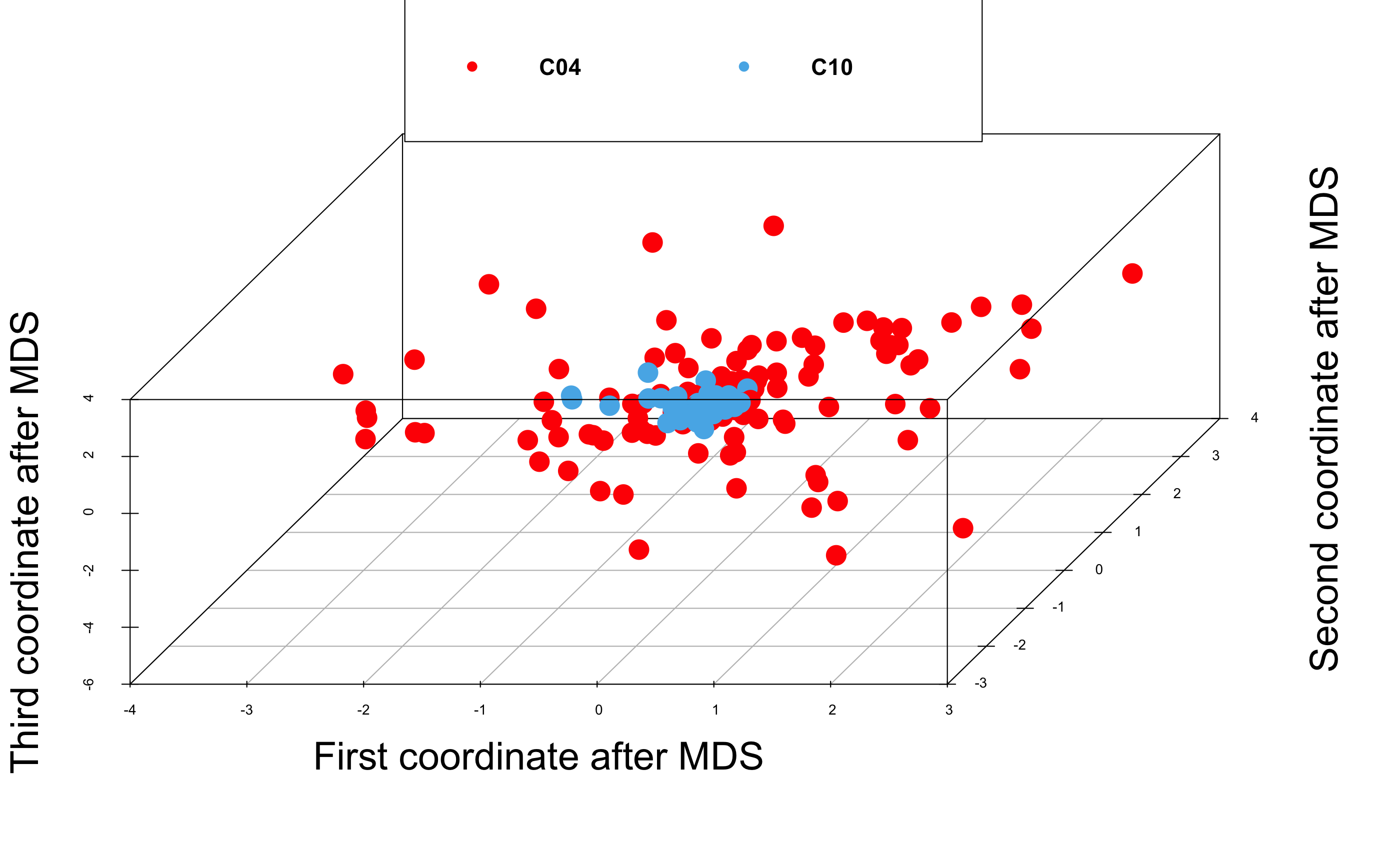
Figure 10: Initialized latent positions $\widehat{U}^{(0)}$

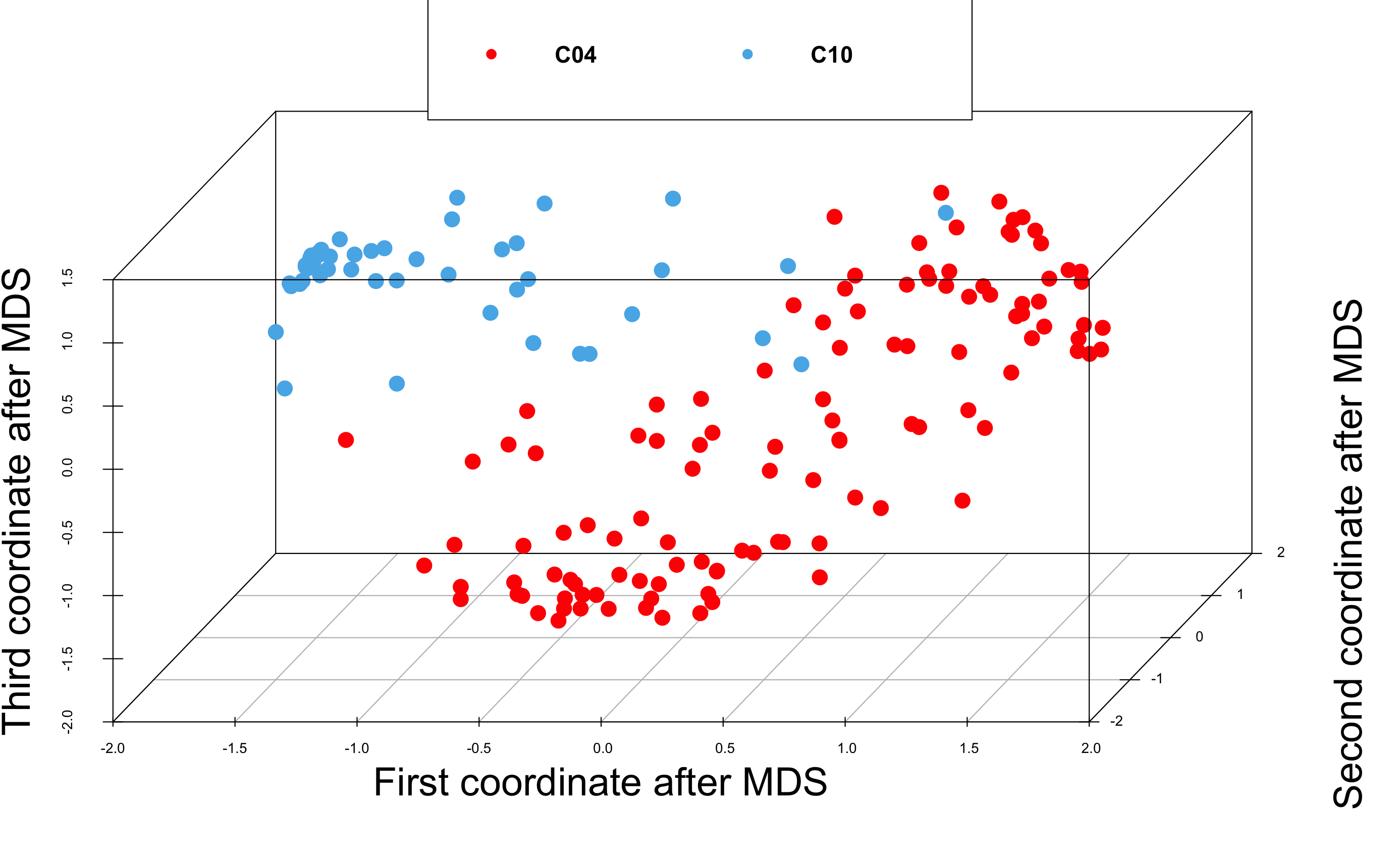
Figure 11: Latent positions $\widehat{U}$ output by Algorithm 1

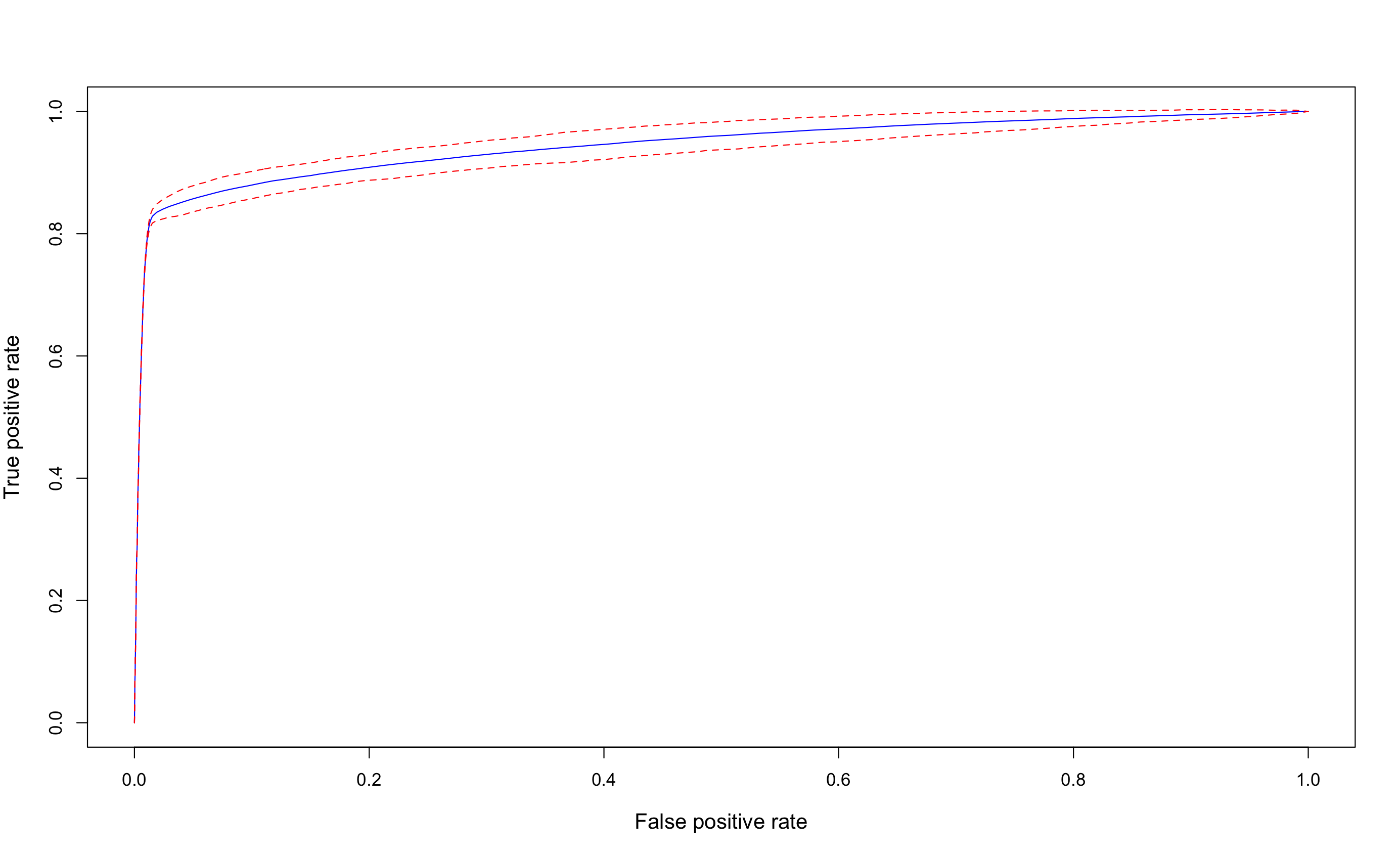
Figure 12: ROC curve for link prediction with $99.9\%$ CI (red dashed line)

7 Concluding remarks

In this paper, we propose a novel unified method for investigating the higher-order interactions in network data. Our framework is general in its abstraction of the concept “layer”, which could be either a third participant in a dyadic relationship/interaction, or it could index the multiple interactions between two nodes, or encode the time stamp in a dynamic network setting. Our model also allows the data generation scheme to connect to the interaction latent positions via a generalized linear link function. It covers several popular mainstream higher-order network models, including multilayer networks, hypergraphs and dynamic networks, as special cases. Our proposed method is therefore versatile and widely applicable. Further, we developed original theory that rigorously guarantees the good performance of the algorithm and quantitatively understand the finite-sample error bounds over our method’s iterations.

There are a number of interesting directions of future work. In this work, we focused on binary network interactions. We expect our algorithm and analysis can be expanded to some weighted edge generation schemes, such as exponential distribution and some sub-Gaussian distributions. But given the volume of work even under the Bernoulli model, we stick to binary edges in this paper and leave the direction for future investigation. Second, we constrain our data generation scheme to generalized linear link functions. While this formulation decently caters to the need of many real-life data analysis tasks, it is interesting to expand the methodology to more general link functions. A third interesting but much more challenging future exploration is to account for dependency between the higher-order interactions.

8 Proofs

For the ease of presentation, throughout the proofs we use $U_{1},U_{2},U_{3}$ to denote $U,V,W$ respectively together with their variants of different superscripts and subscripts (e.g. $U_{k}^{*}$, $U_{k}^{(t)}$ for $k=1,2,3$).

8.1 Proof of Lemma 2

To see the convexity of $\ell_{n}(\mathbf{C}\cdot\llbracket U_{1},U_{2},U_{3}\rrbracket)$, first note that

$$\text{vec}(\mathcal{M}_{1}(\mathbf{C}\times_{1}U_{1}\times_{2}U_{2}\times_{3}U_{3}))=(U_{3}\otimes U_{2}\otimes U_{1})\cdot\text{vec}(\mathcal{M}_{1}(\mathbf{C}))$$

Denote $c_{v}:=\text{vec}(\mathcal{M}_{1}(\mathbf{C}))\in\mathbb{R}^{r_{1}r_{2}r_{3}}$, $\mathring{U}:=U_{3}\otimes U_{2}\otimes U_{1}\in\mathbb{R}^{n_{1}n_{2}n_{3}\times r_{1}r_{2}r_{3}}$ and $\mathring{U}_{ijk}:=U_{3}(k,:)^{T}\otimes U_{2}(j,:)^{T}\otimes U_{1}(i,:)^{T}\in\mathbb{R}^{r_{1}r_{2}r_{3}}$, then the decomposition of $\Theta_{ijk}$ can be written as

$$\Theta_{ijk}=\sum_{l_{1}l_{2}l_{3}}C_{l_{1}l_{2}l_{3}}U_{1}(i,l_{1})U_{2}(j,l_{2})U_{3}(k,l_{3})=\langle c_{v},\mathring{U}_{ijk}\rangle$$

The objective $\ell_{n}(\mathbf{C}\cdot\llbracket U_{1},U_{2},U_{3}\rrbracket)$ essentially becomes

$$f(c_{v}): =-\sum_{ijk}\left[A_{ijk}\log p(\langle c_{v},\mathring{U}_{ijk}\rangle)+(1-A_{ijk})\log(1-p(\langle c_{v},\mathring{U}_{ijk}\rangle))\right]$$

and calculating the hessian of $f(\cdot)$ gives that

$$\nabla^{2}f(c_{v}) =\sum_{ijk}\Bigg{[}A_{ijk}\left(\left(\frac{p^{\prime}(\langle c_{v},\mathring{U}_{ijk}\rangle)}{p(\langle c_{v},\mathring{U}_{ijk}\rangle)}\right)^{2}-\frac{p^{\prime\prime}(\langle c_{v},\mathring{U}_{ijk}\rangle)}{p(\langle c_{v},\mathring{U}_{ijk}\rangle)}\right)$$

$$+(1-A_{ijk})\left(\left(\frac{p^{\prime}(\langle c_{v},\mathring{U}_{ijk}\rangle)}{1-p(\langle c_{v},\mathring{U}_{ijk}\rangle)}\right)^{2}+\frac{p^{\prime\prime}(\langle c_{v},\mathring{U}_{ijk}\rangle)}{1-p(\langle c_{v},\mathring{U}_{ijk}\rangle)}\right)\Bigg{]}\mathring{U}_{ijk}\mathring{U}_{ijk}^{T}$$

For any $x\in\mathbb{R}^{r_{1}r_{2}r_{3}}$ such that $\|x\|_{2}=1$, by Assumption 1 we have

$$\langle\nabla^{2}f(c_{v})x,x\rangle =\sum_{ijk}\Bigg{[}A_{ijk}\left(\left(\frac{p^{\prime}(\langle c_{v},\mathring{U}_{ijk}\rangle)}{p(\langle c_{v},\mathring{U}_{ijk}\rangle)}\right)^{2}-\frac{p^{\prime\prime}(\langle c_{v},\mathring{U}_{ijk}\rangle)}{p(\langle c_{v},\mathring{U}_{ijk}\rangle)}\right)$$

$$+(1-A_{ijk})\left(\left(\frac{p^{\prime}(\langle c_{v},\mathring{U}_{ijk}\rangle)}{1-p(\langle c_{v},\mathring{U}_{ijk}\rangle)}\right)^{2}+\frac{p^{\prime\prime}(\langle c_{v},\mathring{U}_{ijk}\rangle)}{1-p(\langle c_{v},\mathring{U}_{ijk}\rangle)}\right)\Bigg{]}x^{T}\mathring{U}_{ijk}\mathring{U}_{ijk}^{T}x$$

$$\geq\gamma_{\alpha}\sum_{ijk}x^{T}\mathring{U}_{ijk}\mathring{U}_{ijk}^{T}x=\gamma_{\alpha}x^{T}\left(\sum_{ijk}\mathring{U}_{ijk}\mathring{U}_{ijk}^{T}\right)x=\gamma_{\alpha}$$

which implies that $\nabla^{2}f(c_{v})\succeq\gamma_{\alpha}\bm{I}_{r_{1}r_{2}r_{3}}$.

8.2 Proof of Lemma 3

Denote $\mathbf{X}:=\nabla\ell_{n}(\mathbf{\Theta}^{*})-\mathbb{E}\nabla\ell_{n}(\mathbf{\Theta}^{*})$, by the definition of $\textsf{Err}_{\mathbf{r}}$ we have

$$\textsf{Err}_{\mathbf{r}} =\sup_{\begin{subarray}{c}\mathbf{\Theta}\in\mathbb{R}^{n_{1}\times n_{2}\times n_{3}},\|\mathbf{\Theta}\|_{F}\leq 1\\ \text{rank}(\mathbf{\Theta})=(r_{1},r_{2},r_{3})\end{subarray}}\langle X,\mathbf{\Theta}\rangle=\sup_{\begin{subarray}{c}\mathbf{C}\in\mathbb{R}^{r_{1}\times r_{2}\times r_{3}},\|\mathbf{C}\|_{F}\leq 1\\ \|U_{k}\|\leq 1,k=1,2,3\end{subarray}}\langle X,\mathbf{C}\times_{1}U_{1}\times_{2}U_{2}\times_{3}U_{3}\rangle$$

Now we let

$$(\mathbf{C}^{\dagger},U_{1}^{\dagger},U_{2}^{\dagger},U_{3}^{\dagger})=\operatorname*{arg\,max}_{\begin{subarray}{c}\mathbf{C}\in\mathbb{R}^{r_{1}\times r_{2}\times r_{3}},\|\mathbf{C}\|_{F}\leq 1\\ \|U_{k}\|\leq 1,k=1,2,3\end{subarray}}\langle X,\mathbf{C}\times_{1}U_{1}\times_{2}U_{2}\times_{3}U_{3}\rangle$$

and let $\mathcal{N}_{C}^{\epsilon}$ be an $\epsilon$-net of $\{\mathbf{C}\in\mathbb{R}^{r_{1}\times r_{2}\times r_{3}}:\|\mathbf{C}\|_{\rm F}\leq 1\}$ and $\mathcal{N}_{k}^{\epsilon}$ be an $\epsilon$-net of $\{U\in\mathbb{R}^{n_{k}\times r_{k}}:\|U\|\leq 1\}$ for $k=1,2,3$. A simple fact is that

$$\lvert\mathcal{N}_{C}^{\epsilon}\rvert\leq\left(\frac{2+\epsilon}{\epsilon}\right)^{r_{1}r_{2}r_{3}},\quad\lvert\mathcal{N}_{k}^{\epsilon}\rvert\leq\left(\frac{2+\epsilon}{\epsilon}\right)^{n_{k}r_{k}}\text{~{}for~{}}k=1,2,3$$

By the definition of $\epsilon$-net, there exists $\widetilde{\mathbf{C}}\in\mathcal{N}_{C}^{\epsilon}$ and $\widetilde{U}_{k}\in\mathcal{N}_{k}^{\epsilon}$ such that

$$\|\widetilde{C}-C^{\dagger}\|_{\rm F}\leq\epsilon,\quad\|\widetilde{U}_{k}-U_{k}^{\dagger}\|\leq\epsilon$$

Hence we have

$$\textsf{Err}_{\mathbf{r}} =\langle\mathbf{X},\widetilde{}\mathbf{C}\times_{1}\widetilde{U}_{1}\times_{2}\widetilde{U}_{2}\times_{3}\widetilde{U}_{3}\rangle+\langle\mathbf{X},\mathbf{C}^{\dagger}\times_{1}U_{1}^{\dagger}\times_{2}U_{2}^{\dagger}\times_{3}U_{3}^{\dagger}\rangle-\langle\mathbf{X},\widetilde{}\mathbf{C}\times_{1}\widetilde{U}_{1}\times_{2}\widetilde{U}_{2}\times_{3}\widetilde{U}_{3}\rangle$$

$$\leq\langle\mathbf{X},\widetilde{}\mathbf{C}\times_{1}\widetilde{U}_{1}\times_{2}\widetilde{U}_{2}\times_{3}\widetilde{U}_{3}\rangle+4\epsilon\cdot\textsf{Err}_{\mathbf{r}}$$

Note that for any $\mathbf{C}\in\mathcal{N}_{C}^{\epsilon}$ and $U_{k}\in\mathcal{N}_{k}^{\epsilon}$, the Hoeffding inequality gives

$$\mathbb{P}\Big{(}\lvert\langle\mathbf{X},\mathbf{C}\times_{1}U_{1}\times_{2}U_{2}\times_{3}U_{3}\rangle\rvert\geq\frac{t}{2}\Big{)}\leq\exp\left(-{\frac{t^{2}}{2\zeta_{\alpha}^{2}}}\right)$$

where we use $X_{ijk}\in\left\{-\frac{p^{\prime}(\Theta_{ijk})}{p(\Theta_{ijk})},\frac{p^{\prime}(\Theta_{ijk})}{1-p(\Theta_{ijk})}\right\}$ and the definition of $\zeta_{\alpha}$. Now taking $\epsilon=1/8$ and using a union bound, we conclude that

$$\mathbb{P}(\textsf{Err}_{\mathbf{r}}\geq t) \leq\mathbb{P}\Big{(}\max_{\begin{subarray}{c}\mathbf{C}\in N_{C}^{\epsilon}\\ U_{k}\in N_{k}^{\epsilon},k=1,2,3\end{subarray}}\langle\mathbf{X},\mathbf{C}\times_{1}U_{1}\times_{2}U_{2}\times_{3}U_{3}\rangle\geq\frac{t}{2}\Big{)}$$

$$=\mathbb{P}\Big{(}\bigcup_{\begin{subarray}{c}\mathbf{C}\in N_{C}^{\epsilon}\\ U_{k}\in N_{k}^{\epsilon},k=1,2,3\end{subarray}}\left\{\langle\mathbf{X},\mathbf{C}\times_{1}U_{1}\times_{2}U_{2}\times_{3}U_{3}\rangle\geq\frac{t}{2}\right\}\Big{)}$$

$$\leq C^{r_{1}r_{2}r_{3}+\sum_{k=1}^{3}n_{k}r_{k}}\exp\left(-\frac{t^{2}}{2\zeta_{\alpha}^{2}}\right)$$

The proof is completed by adjusting the constant.

8.3 Proof of Theorem 1

8.3.1 Notations and conditions

For the notational simplicity, we interchangeably write $\mathbf{C}^{*}\cdot\llbracket U_{1}^{*},U_{2}^{*},U_{3}^{*}\rrbracket$ and $\mathbf{C}^{*}\times_{1}U_{1}^{*}\times_{2}U_{2}^{*}\times_{3}U_{3}^{*}$ to denote the multilinear product throughout the proof. We denote $O_{k}^{(t)}:=\text{argmin}_{O}\|U^{(t)}-n_{k}^{-1/2}U_{k}^{*}O\|_{\rm F}$, $d_{k}^{(t)}:=d_{\textsf{f}}(U^{(t)},n_{k}^{-1/2}U_{k}^{*})$, and $d_{\textsf{C}}^{(t)}:=\|\mathbf{C}^{(t)}-\mathbf{C}^{*}\cdot\llbracket O_{1}^{(t)\top},O_{2}^{(t)\top},O_{3}^{(t)\top}\rrbracket\|_{\rm F}$. We also denote $\bar{r}=\max_{k}r_{k}$ and

$$\widetilde{U}_{k}^{(t)}:=U^{(t)}-\nabla_{U_{k}}\ell_{n}(\mathbf{\Theta}^{(t)})$$

$$\widetilde{\mathbf{\Theta}}^{(t)}:=(\mathbf{C}^{*}\cdot\llbracket O_{1}^{(t)\top},O_{2}^{(t)\top},O_{3}^{(t)\top}\rrbracket)\times_{1}U_{1}^{(t)}\times_{2}U_{2}^{(t)}\times_{3}U_{3}^{(t)}$$

As we noted before, $U_{k}^{(t)}$ is an estimate of $n_{k}^{-1/2}U_{k}^{*}$. Without loss of generality, throughout the proof we assume $U_{k}^{*}$ is multiplied by the scale factor $n_{k}^{-1/2}$ and the core tensor $\mathbf{C}^{\ast}$ is multiplied by the scale factor $(n_{1}n_{2}n_{3})^{1/2}$. Now we state the conditions in the theorem explicitly. Here $c_{0}$ is some constant to be determined later.

1. $$\textsf{D}_{0}^{2}=\sum_{k=1}^{3}(d_{k}^{(0)})^{2}\leq\frac{c_{1}}{\kappa_{0}^{8}\cdot\bar{r}}$$

   where $c_{1}=\min\left\{c_{1}^{(k)},k=0,\cdots,4\right\}$

   $$c_{1}^{(0)}=\frac{c_{0}^{2}\gamma_{\alpha}^{2}\bar{r}}{12\beta_{\alpha}^{2}},\quad c_{1}^{(1)}=\frac{\bar{r}}{8(2+4\sqrt{\bar{r}})}$$

   $$\quad c_{1}^{(2)}=\frac{\gamma_{\alpha}^{3}\bar{r}}{8\Big{[}\gamma_{\alpha}(1+c_{0})+3(\beta_{\alpha}+1)\Big{]}(\beta_{\alpha}+\gamma_{\alpha})},\quad c_{1}^{(3)}=\frac{c_{2}^{2}\gamma_{\alpha}^{2}}{513^{2}\cdot 128}$$

   $$c_{1}^{(4)}=\frac{\gamma_{\alpha}^{2}\sqrt{\bar{r}}}{16(\beta_{\alpha}+3\gamma_{\alpha})(1+c_{0})^{2}}$$

2. $$\frac{\underline{\Lambda}(\mathbf{C}^{*})}{\textsf{Err}_{\mathbf{r}}}\geq\max\left\{\frac{2}{c_{0}\gamma_{\alpha}},\sqrt{\frac{{256C_{0}^{\prime\prime}c_{3}}}{{\bar{r}}}},\frac{513\sqrt{128C_{0}^{\prime\prime}\bar{r}}}{c_{2}\gamma_{\alpha}}\kappa_{0}^{2},\sqrt{\frac{8{C_{0}}\bar{r}}{c_{1}\gamma_{\alpha}}}\kappa_{0}^{4}\right\}$$

and also

$$\quad c_{3}=\frac{\gamma_{\alpha}^{3}}{384\beta_{\alpha}^{2}(\beta_{\alpha}+\gamma_{\alpha})^{2}(1+c_{0})^{2}}$$

8.3.2 Error of the core tensor $C^{(t)}$

We first focus on iteration $t=1$ and will finalize our proof by induction in the last part (for generality we keep the superscript $t$ here). Notice that $\mathbb{E}\nabla\ell_{n}(\mathbf{\Theta}^{*})=0$. At iteration $t$, $\mathbf{C}^{(t-1)}=\text{argmin}_{\|\mathbf{C}\|_{\rm F}\leq\textsf{Err}_{\mathbf{r}}}\ell_{n}(\mathbf{C}\times_{1}U_{1}^{(t-1)}\times_{2}U_{2}^{(t-1)}\times_{3}U_{3}^{(t-1)})$. By Lemma 2 we have for any $\mathbf{C}\in\mathbb{R}^{r_{1}\times r_{2}\times r_{3}}$

$$\addcontentsline{lla}{section}{\numberline{\string\crtrefnumber{optim_cond}}{o}ptim_{c}ond}\langle\nabla_{\mathbf{C}}\ell_{n}(\mathbf{\Theta}^{(t-1)}),\mathbf{C}^{(t-1)}-\mathbf{C}\rangle\leq 0$$ (12)

where $\nabla_{\mathbf{C}}\ell_{n}(\mathbf{\Theta}^{(t-1)})=\nabla\ell_{n}(\mathbf{\Theta}^{(t-1)})\cdot\llbracket U_{1}^{(t-1)\top},U_{2}^{(t-1)\top},U_{3}^{(t-1)\top}\rrbracket$. Since $\|\mathbf{C}^{(t-1)}\|_{\rm F}\leq\textsf{Err}_{\mathbf{r}}$ and $U_{k}^{(t-1)}$’s are incoherent, we can guarantee that $\|\widetilde{\mathbf{\Theta}}^{(t-1)}\|_{\infty}\leq\alpha$ and $\|\mathbf{\Theta}^{(t-1)}\|_{\infty}\leq\alpha$. Then by Lemma 1 we have

$$\langle\nabla\ell_{n}(\mathbf{\Theta}^{(t-1)})-\nabla\ell_{n}(\widetilde{\mathbf{\Theta}}^{(t-1)}),\mathbf{\Theta}^{(t-1)}-\widetilde{\mathbf{\Theta}}^{(t-1)}\rangle\geq\gamma_{\alpha}\|\mathbf{\Theta}^{(t-1)}-\widetilde{\mathbf{\Theta}}^{(t-1)}\|_{F}^{2}=\gamma_{\alpha}\cdot(d_{\textsf{C}}^{(t-1)})^{2}\addcontentsline{lla}{section}{\numberline{\string\crtrefnumber{eqn0}}{e}qn0}$$ (13)

On the other hand by (12),

$$\langle\nabla\ell_{n}(\mathbf{\Theta}^{(t)}) -\nabla\ell_{n}(\widetilde{\mathbf{\Theta}}^{(t-1)}),\mathbf{\Theta}^{(t-1)}-\widetilde{\mathbf{\Theta}}^{(t-1)}\rangle\leq\langle-\nabla\ell_{n}(\widetilde{\mathbf{\Theta}}^{(t-1)}),\mathbf{\Theta}^{(t-1)}-\widetilde{\mathbf{\Theta}}^{(t-1)}\rangle$$

$$=\langle\nabla\ell_{n}(\mathbf{\Theta}^{*})-\nabla\ell_{n}(\widetilde{\mathbf{\Theta}}^{(t-1)}),\mathbf{\Theta}^{(t-1)}-\widetilde{\mathbf{\Theta}}^{(t-1)}\rangle+\langle\nabla\ell_{n}(\mathbf{\Theta}^{*}),\widetilde{\mathbf{\Theta}}^{(t-1)}-\mathbf{\Theta}^{(t-1)}\rangle$$

The first term above can be bounded as follows:

$$\langle\nabla\ell_{n}(\mathbf{\Theta}^{*})-\nabla\ell_{n}(\widetilde{\mathbf{\Theta}}^{(t-1)}),\mathbf{\Theta}^{(t-1)}-\widetilde{\mathbf{\Theta}}^{(t-1)}\rangle\leq\|\nabla\ell_{n}(\mathbf{\Theta}^{*})-\nabla\ell_{n}(\widetilde{\mathbf{\Theta}})\|_{F}\|\mathbf{\Theta}^{(t-1)}-\widetilde{\mathbf{\Theta}}\|_{F}$$

$$\leq\beta_{\alpha}\|\mathbf{\Theta}^{*}-\widetilde{\mathbf{\Theta}}^{(t-1)}\|_{F}\|\mathbf{\Theta}^{(t-1)}-\widetilde{\mathbf{\Theta}}^{(t-1)}\|_{F}\leq\beta_{\alpha}\|\mathbf{\Theta}^{*}-\widetilde{\mathbf{\Theta}}^{(t-1)}\|_{F}\cdot d_{\textsf{C}}^{(t-1)}$$

$$\leq\beta_{\alpha}\|\mathbf{C}^{*}\cdot\llbracket U_{1}^{*},U_{2}^{*},U_{3}^{*}\rrbracket-\mathbf{C}^{*}\cdot\llbracket U_{1}^{(t-1)}O_{1}^{(t-1)\top},U_{2}^{(t-1)}O_{2}^{(t-1)\top},U_{3}^{(t-1)}O_{3}^{(t-1)\top}\rrbracket\|_{\text{F}}\cdot d_{\textsf{C}}^{(t-1)}$$

$$\leq\beta_{\alpha}\overline{\Lambda}(\mathbf{C}^{*})\cdot d_{\textsf{C}}^{(t-1)}\cdot\sum_{k=1}^{3}d_{k}^{(t-1)}\addcontentsline{lla}{section}{\numberline{\string\crtrefnumber{eqn1}}{e}qn1}$$ (14)

The second term can bounded as follows:

$$\langle\nabla\ell_{n}(\mathbf{\Theta}^{*}),\widetilde{\mathbf{\Theta}}^{(t-1)}-\mathbf{\Theta}^{(t-1)}\rangle=\langle\nabla\ell_{n}(\mathbf{\Theta}^{*})-\nabla L(\mathbf{\Theta}^{*}),\widetilde{\mathbf{\Theta}}^{(t-1)}-\mathbf{\Theta}^{(t-1)}\rangle$$

$$\leq\|\left(\nabla\ell_{n}(\mathbf{\Theta}^{*})-\nabla L(\mathbf{\Theta}^{*})\right)\times_{1}(U_{1}^{(t-1)})^{\top}\times_{2}(U_{2}^{(t-1)})^{\top}\times_{3}(U_{3}^{(t-1)})^{\top}\|_{F}\cdot d_{\textsf{C}}^{(t-1)}$$

$$=\sup_{\begin{subarray}{c}\mathbf{C}\in\mathbb{R}^{r_{1}\times r_{2}\times r_{3}},\|\mathbf{C}\|_{F}\leq 1\end{subarray}}\langle\left(\nabla\ell_{n}(\mathbf{\Theta}^{*})-\nabla L(\mathbf{\Theta}^{*})\right),\mathbf{C}\times_{1}U_{1}^{(t-1)}\times_{2}U_{2}^{(t-1)}\times_{3}U_{3}^{(t-1)}\rangle\cdot d_{\textsf{C}}^{(t-1)}$$

$$\leq\textsf{Err}_{\mathbf{r}}\cdot d_{\textsf{C}}^{(t-1)}\addcontentsline{lla}{section}{\numberline{\string\crtrefnumber{eqn2}}{e}qn2}$$ (15)

Combining (13), (14) and (15) we have

$$d_{\textsf{C}}^{(t-1)}\leq\frac{\beta_{\alpha}}{\gamma_{\alpha}}\cdot\overline{\Lambda}(\mathbf{C}^{*})\cdot\sum_{k=1}^{3}d_{k}^{(t-1)}+\frac{\textsf{Err}_{\mathbf{r}}}{\gamma_{\alpha}}\addcontentsline{lla}{section}{\numberline{\string\crtrefnumber{Cerror}}{C}error}$$ (16)

which hold for $t=1$.

8.3.3 Error of $\widetilde{U}_{k}^{(t)}$ (Gradient descent step)

By (16) and the condition (a) and (b), we have

$$\sum_{k=1}^{3}d_{k}^{(t-1)}\leq\sqrt{3\sum_{k=1}^{3}(d_{k}^{(t-1)})^{2}}\leq\frac{c_{0}\gamma_{\alpha}}{2\beta_{\alpha}\kappa_{0}^{2}},\quad\underline{\Lambda}(\mathbf{C}^{*})\geq\frac{2\textsf{Err}_{\mathbf{r}}}{\gamma_{\alpha}c_{0}}\addcontentsline{lla}{section}{\numberline{\string\crtrefnumber{dklambdacond}}{d}klambdacond}$$ (17)

and the following inequality which will be used throughout this section:

$$\overline{\Lambda}(\mathbf{C}^{(t)})\leq(1+c_{0})\overline{\Lambda}(\mathbf{C}^{*}),\quad\underline{\Lambda}(\mathbf{C}^{(t)})\geq(1+c_{0})\underline{\Lambda}(\mathbf{C}^{*})\addcontentsline{lla}{section}{\numberline{\string\crtrefnumber{CtCstarrel}}{C}tCstarrel}$$ (18)

WLOG we consider the case $k=1$. Note that at iteration $t$, we have

$$\|\widetilde{U}_{1}^{(t)}-{U}_{1}^{*}O_{1}^{(t-1)}\|_{F}^{2} =\|{U}_{1}^{(t)}-\eta\mathcal{M}_{1}(\nabla\ell_{n}(\mathbf{\Theta}^{(t-1)}))(U_{3}^{(t-1)}\otimes U_{2}^{(t-1)})\mathcal{M}_{1}^{T}(\mathbf{C}^{(t-1)})-{U}_{k}^{*}O_{1}^{(t-1)}\|_{F}^{2}$$

$$=(d_{1}^{(t)})^{2}+\eta^{2}\|\mathcal{M}_{1}(\nabla\ell_{n}(\mathbf{\Theta}^{(t-1)}))(U_{3}^{(t-1)}\otimes U_{2}^{(t-1)})\mathcal{M}_{1}^{T}(\mathbf{C}^{(t-1)})\|_{F}^{2}$$

$$-2\eta\langle{U}_{1}^{(t)}-{U}_{k}^{*}O_{1}^{(t-1)},\mathcal{M}_{1}(\nabla\ell_{n}(\mathbf{\Theta}^{(t-1)}))(U_{3}^{(t-1)}\otimes U_{2}^{(t-1)})\mathcal{M}_{1}^{T}(\mathbf{C}^{(t-1)})\rangle$$

Then we bound the last two terms separately. Note that

$$\eta^{2}\|\mathcal{M}_{1}(\nabla\ell_{n}(\mathbf{\Theta}^{(t-1)}))(U_{3}^{(t-1)}\otimes U_{2}^{(t-1)})\mathcal{M}_{1}^{T}(\mathbf{C}^{(t-1)})\|_{F}^{2}$$

$$\leq 2\eta^{2}\|\mathcal{M}_{1}(\nabla\ell_{n}(\mathbf{\Theta}^{*}))(U_{3}^{(t-1)}\otimes U_{2}^{(t-1)})\mathcal{M}_{1}^{T}(\mathbf{C}^{(t-1)})\|_{F}^{2}$$

$$+2\eta^{2}\|\mathcal{M}_{1}(\nabla\ell_{n}(\mathbf{\Theta}^{(t-1)})-\nabla\ell_{n}(\mathbf{\Theta}^{*}))(U_{3}^{(t-1)}\otimes U_{2}^{(t-1)})\mathcal{M}_{1}^{T}(\mathbf{C}^{(t-1)})\|_{F}^{2}$$

$$\leq 2\eta^{2}\|\mathcal{M}_{1}(\mathbf{C}^{(t-1)})\|^{2}\textsf{Err}_{\mathbf{r}}^{2}+2\eta^{2}\beta_{\alpha}^{2}\|\mathbf{\Theta}^{(t-1)}-\mathbf{\Theta}^{*}\|_{F}^{2}\|\mathcal{M}_{1}(\mathbf{C}^{(t-1)})\|^{2}$$

$$\leq{2\eta^{2}\overline{\Lambda}^{2}(\mathbf{C}^{(t-1)})\left[\textsf{Err}_{\mathbf{r}}^{2}+\beta_{\alpha}^{2}\left(d_{\textsf{C}}^{(t-1)}+\overline{\Lambda}(\mathbf{C}^{*})\sum_{k=1}^{3}d_{k}^{(t-1)}\right)^{2}\right]}$$

$$\leq\frac{8\beta_{\alpha}^{2}(\beta_{\alpha}+\gamma_{\alpha})^{2}(1+c_{0})^{2}\overline{\Lambda}^{4}(\mathbf{C}^{*})}{\gamma_{\alpha}^{2}}\eta^{2}\cdot\sum_{k=1}^{3}(d_{k}^{(t-1)})^{2}+\frac{(8\beta_{\alpha}^{2}+2\gamma_{\alpha}^{2})(1+c_{0})^{2}\overline{\Lambda}^{2}(\mathbf{C}^{*})}{\gamma_{\alpha}^{2}}\eta^{2}\textsf{Err}_{\mathbf{r}}^{2}=:A$$

Similarly we could derive the bound for $k=2$ and $k=3$. Therefore, we can write

$$\sum_{k=1}^{3}\|\widetilde{U}_{k}^{(t)}-{U}_{k}^{*}O_{k}^{(t-1)}\|_{F}^{2} \leq\sum_{k=1}^{3}(d_{k}^{(t-1)})^{2}+3A-2\eta\langle\nabla\ell_{n}(\mathbf{\Theta}^{(t-1)}),B_{0}+B_{1}+B_{2}+B_{3}+B_{4}\rangle\addcontentsline{lla}{section}{\numberline{\string\crtrefnumber{UB01234}}{U}B01234}$$ (19)

where

$$B_{0}=\mathbf{C}^{(t-1)}\cdot\llbracket U_{1}^{(t-1)},U_{2}^{(t-1)},U_{3}^{(t-1)}\rrbracket-\mathbf{C}^{*}\cdot\llbracket U_{1}^{*},U_{2}^{*},U_{3}^{*}\rrbracket$$

$$B_{1}=\mathbf{C}^{(t-1)}\cdot\llbracket U_{1}^{(t-1)}-U_{1}^{*}O_{1}^{(t-1)},U_{2}^{(t-1)}-U_{2}^{*}O_{2}^{(t-1)},U_{3}^{(t-1)}\rrbracket$$

$$B_{2}=\mathbf{C}^{(t-1)}\cdot\llbracket U_{1}^{(t-1)}-U_{1}^{*}O_{1}^{(t-1)},U_{2}^{(t-1)},U_{3}^{(t-1)}-U_{3}^{*}O_{3}^{(t-1)}\rrbracket$$

$$B_{3}=\mathbf{C}^{(t-1)}\cdot\llbracket U_{1}^{(t-1)},U_{2}^{(t-1)}-U_{2}^{*}O_{2}^{(t-1)},U_{3}^{(t-1)}-U_{3}^{*}O_{3}^{(t-1)}\rrbracket$$

$$B_{4}=\left[\mathbf{C}^{*}-\mathbf{C}^{(t-1)}\cdot\llbracket O_{1}^{(t-1)},O_{2}^{(t-1)},O_{3}^{(t-1)}\rrbracket\right]\cdot\llbracket U_{1}^{*},U_{2}^{*},U_{2}^{*}\rrbracket$$

We are going to bound $\langle\nabla\ell_{n}(\mathbf{\Theta}^{(t-1)}),B_{0}+B_{1}+B_{2}+B_{3}+B_{4}\rangle$ separately. First note that

$$\langle\nabla\ell_{n}(\mathbf{\Theta}^{(t-1)}),B_{0}\rangle =\langle\nabla\ell_{n}(\mathbf{\Theta}^{(t-1)})-\nabla\ell_{n}(\mathbf{\Theta}^{*}),\mathbf{\Theta}^{(t-1)}-\mathbf{\Theta}^{*}\rangle+\langle\nabla\ell_{n}(\mathbf{\Theta}^{*})-\nabla L(\mathbf{\Theta}^{*}),\mathbf{\Theta}^{(t-1)}-\mathbf{\Theta}^{*}\rangle$$

$$\geq\gamma_{\alpha}\|\mathbf{\Theta}^{(t-1)}-\mathbf{\Theta}^{*}\|_{F}^{2}-|\langle\nabla\ell_{n}(\mathbf{\Theta}^{*})-\nabla L(\mathbf{\Theta}^{*}),\mathbf{\Theta}^{(t-1)}-\mathbf{\Theta}^{*}\rangle|\addcontentsline{lla}{section}{\numberline{\string\crtrefnumber{eqn3}}{e}qn3}$$ (20)

where we need to expand the $\|\mathbf{\Theta}^{(t-1)}-\mathbf{\Theta}^{*}\|_{F}^{2}$ to find a lower bound of it. Denote $\Delta_{k}:=U_{k}^{(t-1)}O_{k}^{(t-1)T}-U_{k}^{*}$ for $k=1,2,3$ and $\Delta_{C}:=\mathbf{C}^{(t-1)}-\mathbf{C}^{*}\cdot\llbracket O_{1}^{(t-1)\top},O_{2}^{(t-1)\top},O_{3}^{(t-1)\top}\rrbracket$ then we have

$$\|\mathbf{\Theta}^{(t-1)}-\mathbf{\Theta}^{*}\|_{F}^{2}=\|\mathbf{\Theta}^{(t-1)}-\widetilde{\mathbf{\Theta}}^{(t-1)}+\widetilde{\mathbf{\Theta}}^{(t-1)}-\mathbf{\Theta}^{*}\|_{F}^{2}$$

$$=\big{\|}\mathbf{\Theta}^{(t-1)}-\widetilde{\mathbf{\Theta}}^{(t-1)}+\underbrace{\mathbf{C}^{*}\cdot\llbracket{\Delta_{1}},U_{2}^{(t-1)}O_{2}^{(t-1)\top},U_{3}^{(t-1)}O_{3}^{(t-1)\top}\rrbracket}_{B_{01}}$$

$$+\underbrace{\mathbf{C}^{*}\cdot\llbracket U_{1}^{*},{\Delta_{2}},U_{3}^{(t-1)}O_{3}^{(t-1)\top}\rrbracket}_{B_{02}}+\underbrace{\mathbf{C}^{*}\cdot\llbracket U_{1}^{*},U_{2}^{*},{\Delta_{3}}\rrbracket}_{B_{03}}\big{\|}_{F}^{2}$$

$$=\big{\|}\mathbf{\Theta}^{(t-1)}-\widetilde{\mathbf{\Theta}}^{(t-1)}\big{\|}_{F}^{2}+\sum_{k=1}^{3}\|B_{0k}\|_{F}^{2}+2\sum_{k=1}^{3}\langle\mathbf{\Theta}^{(t-1)}-\widetilde{\mathbf{\Theta}}^{(t-1)},B_{0k}\rangle+2\sum_{k,l\in[3],k\neq l}\langle B_{0k},B_{0l}\rangle\addcontentsline{lla}{section}{\numberline{\string\crtrefnumber{eqn4}}{e}qn4}$$ (21)

Note that the first term on the RHS of (21) is nothing but $(d_{\textsf{C}}^{(t-1)})^{2}$ and moreover,

$$\|B_{01}\|_{F}^{2}=\|\Delta_{1}\mathcal{M}(\mathbf{C}^{*})(U_{3}^{(t-1)}O_{3}^{(t-1)}\otimes U_{2}^{(t-1)}O_{2}^{(t-1)})^{\top}\|_{F}^{2}=\|\Delta_{1}\mathcal{M}(\mathbf{C}^{*})\|_{F}^{2}\geq\underline{\Lambda}^{2}(\mathbf{C}^{*})(d_{1}^{(t-1)})^{2}$$

Similar bounds holds for $\|B_{02}\|_{F}^{2}$ and $\|B_{03}\|_{F}^{2}$, then we have the lower bound for the second term

$$\sum_{k=1}^{3}\|B_{0k}\|_{F}^{2}\geq\underline{\Lambda}^{2}(\mathbf{C}^{*})\sum_{k=1}^{3}(d_{k}^{(t-1)})^{2}\addcontentsline{lla}{section}{\numberline{\string\crtrefnumber{eqn5}}{e}qn5}$$ (22)

For the third term of (21), note that

$$|\langle\mathbf{\Theta}^{(t-1)}-\widetilde{\mathbf{\Theta}}^{(t-1)},B_{01}\rangle|$$

$$=|\langle\mathcal{M}_{1}(\Delta_{C})(U_{3}^{(t-1)}\otimes U_{2}^{(t-1)}),U_{1}^{(t-1)T}\Delta_{1}\mathcal{M}_{1}(\mathbf{C}^{*})(U_{3}^{(t-1)}O_{3}^{(t-1)}\otimes U_{2}^{(t-1)}O_{2}^{(t-1)})\rangle|$$

$$\leq{\overline{\Lambda}}(\mathbf{C}^{*})d_{\textsf{C}}^{(t-1)}\|U_{1}^{(t-1)T}\Delta_{1}\|_{F}\leq{\overline{\Lambda}}(\mathbf{C}^{*})d_{\textsf{C}}^{(t-1)}(d_{1}^{(t-1)})^{2}$$

where the last inequality can be found in, e.g., Xia and Yuan (2019). Therefore, we have

$$2\sum_{k=1}^{3}|\langle\mathbf{\Theta}^{(t-1)}-\widetilde{\mathbf{\Theta}}^{(t-1)},B_{0k}\rangle|\leq 2{\overline{\Lambda}}(\mathbf{C}^{*})d_{\textsf{C}}^{(t-1)}\sum_{k=1}^{3}(d_{k}^{(t-1)})^{2}\addcontentsline{lla}{section}{\numberline{\string\crtrefnumber{eqn6}}{e}qn6}$$ (23)

For the last term of (21), note that

$$|\langle B_{01},B_{02}\rangle| =|\langle\Delta_{1}\mathcal{M}_{1}(\mathbf{C}^{*})(U_{3}^{(t-1)}O_{3}^{(t-1)T}\otimes U_{2}^{(t-1)}O_{2}^{(t-1)T}),U_{1}^{*}\mathcal{M}_{1}(\mathbf{C}^{*})(U_{3}^{(t-1)}O_{3}^{(t-1)T}\otimes\Delta_{2})\rangle|$$

$$=|\langle\mathcal{M}_{1}(\mathbf{C}^{*})(I_{r_{3}}\otimes U_{2}^{(t-1)T}O_{2}^{(t-1)}\Delta_{2}),\Delta_{1}^{T}U_{1}^{*}\mathcal{M}_{1}(\mathbf{C}^{*})\rangle|$$

$$\leq\sqrt{r_{3}}\bar{\Lambda}^{2}(\mathbf{C}^{*})(d_{1}^{(t-1)})^{2}(d_{2}^{(t-1)})^{2}$$

Therefore we have

$$2\sum_{k,l\in[3],k\neq l}|\langle B_{0k},B_{0l}\rangle| \leq 2{\overline{\Lambda}}^{2}(\mathbf{C}^{*})\sqrt{\bar{r}}\left((d_{1}^{(t-1)}d_{2}^{(t-1)})^{2}+(d_{1}^{(t-1)}d_{3}^{(t-1)})^{2}+(d_{2}^{(t-1)}d_{3}^{(t-1)})^{2}\right)$$

$$\leq 2{\overline{\Lambda}}^{2}(\mathbf{C}^{*})\sqrt{\bar{r}}\sum_{k=1}^{3}(d_{k}^{(t-1)})^{4}\addcontentsline{lla}{section}{\numberline{\string\crtrefnumber{eqn7}}{e}qn7}$$ (24)

In addition, similar to (15), the second term of (20) can be bounded as

$$|\langle\nabla\ell_{n}(\mathbf{\Theta}^{*})-\nabla L(\mathbf{\Theta}^{*}),\mathbf{\Theta}^{(t-1)}-\mathbf{\Theta}^{*}\rangle|\leq\left(d_{\textsf{C}}^{(t-1)}+{\overline{\Lambda}}(\mathbf{C}^{*})\sum_{k=1}^{3}d_{k}^{(t-1)}\right)\cdot\textsf{Err}_{\mathbf{r}}\addcontentsline{lla}{section}{\numberline{\string\crtrefnumber{eqn8}}{e}qn8}$$ (25)

Combining (20) to (25), we have

$$\langle\nabla\ell_{n}(\mathbf{\Theta}^{(t-1)}),B_{0}\rangle \geq\gamma_{\alpha}\Big{[}(d_{\textsf{C}}^{(t-1)})^{2}+\underline{\Lambda}^{2}(\mathbf{C}^{*})\sum_{k=1}^{3}(d_{k}^{(t-1)})^{2}-2{\overline{\Lambda}}(\mathbf{C}^{*})d_{\textsf{C}}^{(t-1)}\sum_{k=1}^{3}(d_{k}^{(t-1)})^{2}$$

$$-2{\overline{\Lambda}}^{2}(\mathbf{C}^{*})\sqrt{\bar{r}}\sum_{k=1}^{3}(d_{k}^{(t-1)})^{4}\Big{]}-\left(d_{\textsf{C}}^{(t-1)}+{\overline{\Lambda}}(\mathbf{C}^{*})\sum_{k=1}^{3}d_{k}^{(t-1)}\right)\cdot\textsf{Err}_{\mathbf{r}}\addcontentsline{lla}{section}{\numberline{\string\crtrefnumber{B0}}{B}0}$$ (26)

Next, notice that

$$|\langle\nabla\ell_{n}(\mathbf{\Theta}^{(t-1)}),\sum_{k=1}^{3}B_{k}\rangle| \leq|\langle\nabla\ell_{n}(\mathbf{\Theta}^{(t-1)})-\nabla\ell_{n}(\mathbf{\Theta}^{*}),\sum_{k=1}^{3}B_{k}\rangle|+|\langle\nabla\ell_{n}(\mathbf{\Theta}^{*}),\sum_{k=1}^{3}B_{k}\rangle|$$

$$\leq\beta_{\alpha}\|\mathbf{\Theta}^{(t-1)}-\mathbf{\Theta}^{*}\|_{F}\big{\|}\sum_{k=1}^{3}B_{k}\big{\|}_{F}+|\langle\nabla\ell_{n}(\mathbf{\Theta}^{*}),\sum_{k=1}^{3}B_{k}\rangle|$$

$$\leq\beta_{\alpha}\left(d_{\textsf{C}}^{(t-1)}+{\overline{\Lambda}}(\mathbf{C}^{*})\sum_{k=1}^{3}d_{k}^{(t-1)}\right)\sum_{k=1}^{3}\|B_{k}\|_{F}+|\langle\nabla\ell_{n}(\mathbf{\Theta}^{*}),\sum_{k=1}^{3}B_{k}\rangle|$$

By the definition of $\{B_{k}\}_{k=1}^{3}$, we have

$$\sum_{k=1}^{3}\|B_{k}\|_{F} \leq\overline{\Lambda}(\mathbf{C}^{(t-1)})\left(d_{1}^{(t-1)}d_{2}^{(t-1)}+d_{1}^{(t-1)}d_{3}^{(t-1)}+d_{2}^{(t-1)}d_{2}^{(t-1)}\right)\leq\overline{\Lambda}(\mathbf{C}^{(t-1)})\sum_{k=1}^{3}(d_{k}^{(t-1)})^{2}$$

And a similar argument to (15) gives that

$$|\langle\nabla\ell_{n}(\mathbf{\Theta}^{*}),\sum_{k=1}^{3}B_{k}\rangle| \leq\overline{\Lambda}(\mathbf{C}^{(t-1)})\cdot\textsf{Err}_{\mathbf{r}}\cdot\left(d_{1}^{(t-1)}d_{2}^{(t-1)}+d_{1}^{(t-1)}d_{3}^{(t-1)}+d_{2}^{(t-1)}d_{2}^{(t-1)}\right)\leq\overline{\Lambda}(\mathbf{C}^{(t-1)})\cdot\textsf{Err}_{\mathbf{r}}\cdot\sum_{k=1}^{3}(d_{k}^{(t-1)})^{2}$$

Therefore, we have

$$|\langle\nabla\ell_{n}(\mathbf{\Theta}^{(t-1)}),\sum_{k=1}^{3}B_{k}\rangle| \leq\overline{\Lambda}(\mathbf{C}^{(t-1)})\left[\beta_{\alpha}d_{\textsf{C}}^{(t-1)}+\beta_{\alpha}{\overline{\Lambda}}(\mathbf{C}^{*})\sum_{k=1}^{3}d_{k}^{(t-1)}+\textsf{Err}_{\mathbf{r}}\right]\cdot\sum_{k=1}^{3}(d_{k}^{(t-1)})^{2}\addcontentsline{lla}{section}{\numberline{\string\crtrefnumber{B123}}{B}123}$$ (27)

It remains to upper bound $-\langle\nabla\ell_{n}(\mathbf{\Theta}^{(t-1)}),B_{4}\rangle$. Observe that

$$-\langle\nabla\ell_{n}(\mathbf{\Theta}^{(t-1)}),B_{4}\rangle=\langle\nabla\ell_{n}(\mathbf{\Theta}^{(t-1)}),\left[\mathbf{C}^{(t-1)}\cdot\llbracket O_{1}^{(t-1)},O_{2}^{(t-1)},O_{3}^{(t-1)}\rrbracket-\mathbf{C}^{*}\right]\cdot\llbracket U_{1}^{*},U_{2}^{*},U_{2}^{*}\rrbracket\rangle$$

$$=\langle\nabla\ell_{n}(\mathbf{\Theta}^{(t-1)}),\underbrace{\Delta_{C}\cdot\llbracket U_{1}^{*}O_{1}^{(t-1)},U_{2}^{*}O_{2}^{(t-1)},U_{3}^{*}O_{3}^{(t-1)}\rrbracket-\Delta_{C}\cdot\llbracket U_{1}^{(t-1)},U_{2}^{(t-1)},U_{3}^{(t-1)}\rrbracket}_{B_{40}}\rangle$$

$$+\langle\nabla\ell_{n}(\mathbf{\Theta}^{(t-1)}),\Delta_{C}\cdot\llbracket U_{1}^{(t-1)},U_{2}^{(t-1)},U_{3}^{(t-1)}\rrbracket\rangle$$

$$\leq\langle\nabla\ell_{n}(\mathbf{\Theta}^{(t-1)}),B_{40}\rangle=\langle\nabla\ell_{n}(\mathbf{\Theta}^{(t-1)})-\nabla\ell_{n}(\mathbf{\Theta}^{*}),{B_{40}}\rangle+\langle\nabla\ell_{n}(\mathbf{\Theta}^{*}),{B_{40}}\rangle$$

$$\leq\beta_{\alpha}\|\mathbf{\Theta}^{(t-1)}-\mathbf{\Theta}^{*}\|_{F}\cdot d_{\textsf{C}}^{(t-1)}\sum_{k=1}^{3}d_{k}^{(t-1)}+\textsf{Err}_{\mathbf{r}}\cdot d_{\textsf{C}}^{(t-1)}\sum_{k=1}^{3}d_{k}^{(t-1)}$$

$$\leq\left[\beta_{\alpha}d_{\textsf{C}}^{(t-1)}+\beta_{\alpha}{\overline{\Lambda}}(\mathbf{C}^{*})\sum_{k=1}^{3}d_{k}^{(t-1)}+\textsf{Err}_{\mathbf{r}}\right]d_{\textsf{C}}^{(t-1)}\cdot\sum_{k=1}^{3}d_{k}^{(t-1)}\addcontentsline{lla}{section}{\numberline{\string\crtrefnumber{B4}}{B}4}$$ (28)

where the first inequality is due to the optimality condition (12), and the third inequality follows from the following decomposition

$$B_{40}= \Delta_{C}\cdot\Big{[}\llbracket-\Delta_{1}O_{1}^{(t-1)},U_{2}^{*}O_{2}^{(t-1)},U_{3}^{*}O_{3}^{(t-1)}\rrbracket+\llbracket U_{1}^{(t-1)},-\Delta_{2}O_{2}^{(t-1)},U_{3}^{*}O_{3}^{(t-1)}\rrbracket$$

$$+\llbracket U_{1}^{(t-1)},U_{2}^{(t-1)},-\Delta_{3}O_{3}^{(t-1)}\rrbracket\Big{]}$$

Combining (16), (26), (27) and (28) we have

$$-2\eta\langle\nabla\ell_{n}(\mathbf{\Theta}^{(t-1)}),B_{0}+B_{1}+B_{2}+B_{3}+B_{4}\rangle\leq-2\eta\gamma_{\alpha}\Big{[}(d_{\textsf{C}}^{(t-1)})^{2}+\underline{\Lambda}^{2}(\mathbf{C}^{*})\sum_{k=1}^{3}(d_{k}^{(t-1)})^{2}$$

$$-2{\overline{\Lambda}}(\mathbf{C}^{*})d_{\textsf{C}}^{(t-1)}\sum_{k=1}^{3}(d_{k}^{(t-1)})^{2}-2{\overline{\Lambda}}^{2}(\mathbf{C}^{*})\sqrt{\bar{r}}\sum_{k=1}^{3}(d_{k}^{(t-1)})^{4}\Big{]}+2\eta\left(d_{\textsf{C}}^{(t-1)}+{\overline{\Lambda}}(\mathbf{C}^{*})\sum_{k=1}^{3}d_{k}^{(t-1)}\right)\cdot\textsf{Err}_{\mathbf{r}}$$

$$+2\eta\overline{\Lambda}(\mathbf{C}^{(t-1)})\left[\beta_{\alpha}d_{\textsf{C}}^{(t-1)}+\beta_{\alpha}{\overline{\Lambda}}(\mathbf{C}^{*})\sum_{k=1}^{3}d_{k}^{(t-1)}+\textsf{Err}_{\mathbf{r}}\right]\cdot\sum_{k=1}^{3}(d_{k}^{(t-1)})^{2}$$

$$+2\eta\left[\beta_{\alpha}d_{\textsf{C}}^{(t-1)}+\beta_{\alpha}{\overline{\Lambda}}(\mathbf{C}^{*})\sum_{k=1}^{3}d_{k}^{(t-1)}+\textsf{Err}_{\mathbf{r}}\right]d_{\textsf{C}}^{(t-1)}\cdot\sum_{k=1}^{3}d_{k}^{(t-1)}$$

$$\leq-2\eta\gamma_{\alpha}\underline{\Lambda}^{2}(\mathbf{C}^{*})\sum_{k=1}^{3}(d_{k}^{(t-1)})^{2}+(2+4\sqrt{\bar{r}})\gamma_{\alpha}{\overline{\Lambda}}^{2}(\mathbf{C}^{*})\eta\cdot\sum_{k=1}^{3}(d_{k}^{(t-1)})^{2}\cdot\sum_{k=1}^{3}(d_{k}^{(t-1)})^{2}$$

$$+\frac{2(\beta_{\alpha}+\gamma_{\alpha}){\overline{\Lambda}}(\mathbf{C}^{*})}{\gamma_{\alpha}}\eta\textsf{Err}_{\mathbf{r}}\cdot\sum_{k=1}^{3}d_{k}^{(t-1)}+\frac{2}{\gamma_{\alpha}}\eta\textsf{Err}_{\mathbf{r}}^{2}+\frac{2\beta_{\alpha}(\beta_{\alpha}+\gamma_{\alpha})(1+c_{0}){\overline{\Lambda}}^{2}(\mathbf{C}^{*})}{\gamma_{\alpha}}\eta\cdot\sum_{k=1}^{3}d_{k}^{(t-1)}\cdot\sum_{k=1}^{3}(d_{k}^{(t-1)})^{2}$$

$$+\frac{2(\beta_{\alpha}+\gamma_{\alpha})(1+c_{0})\overline{\Lambda}(\mathbf{C}^{*})}{\gamma_{\alpha}}\eta\textsf{Err}_{\mathbf{r}}\cdot\sum_{k=1}^{3}(d_{k}^{(t-1)})^{2}+\frac{6\beta_{\alpha}(\beta_{\alpha}+\gamma_{\alpha}){\overline{\Lambda}}^{2}(\mathbf{C}^{*})}{\gamma_{\alpha}^{2}}\eta\cdot\sum_{k=1}^{3}d_{k}^{(t-1)}\cdot\sum_{k=1}^{3}(d_{k}^{(t-1)})^{2}$$

$$+\frac{6\beta_{\alpha}(\beta_{\alpha}+\gamma_{\alpha}){\overline{\Lambda}}(\mathbf{C}^{*})}{\gamma_{\alpha}^{2}}\eta\textsf{Err}_{\mathbf{r}}\cdot\sum_{k=1}^{3}(d_{k}^{(t-1)})^{2}+\frac{6(\beta_{\alpha}+\gamma_{\alpha}){\overline{\Lambda}}(\mathbf{C}^{*})}{\gamma_{\alpha}^{2}}\eta\textsf{Err}_{\mathbf{r}}\cdot\sum_{k=1}^{3}(d_{k}^{(t-1)})^{2}+\frac{2(\beta_{\alpha}+\gamma_{\alpha})}{\gamma_{\alpha}^{2}}\eta\textsf{Err}_{\mathbf{r}}^{2}\cdot\sum_{k=1}^{3}d_{k}^{(t-1)}$$

$$\leq-2\eta\gamma_{\alpha}\underline{\Lambda}^{2}(\mathbf{C}^{*})\sum_{k=1}^{3}(d_{k}^{(t-1)})^{2}+\frac{\gamma_{\alpha}{\overline{\Lambda}}^{2}(\mathbf{C}^{*})}{\kappa_{0}^{2}}\eta\sum_{k=1}^{3}(d_{k}^{(t-1)})^{2}$$

$$+\Big{[}(2+4\sqrt{\bar{r}})\gamma_{\alpha}+\frac{\Big{[}\gamma_{\alpha}(1+c_{0})+3(\beta_{\alpha}+1)\Big{]}(\beta_{\alpha}+\gamma_{\alpha})}{\gamma_{\alpha}^{2}}\Big{]}{\overline{\Lambda}}^{2}(\mathbf{C}^{*})\eta\cdot\sum_{k=1}^{3}(d_{k}^{(t-1)})^{2}\cdot\sum_{k=1}^{3}(d_{k}^{(t-1)})^{2}$$

$$+\frac{\Big{[}2\gamma_{\alpha}(1+c_{0})+6\Big{]}\beta_{\alpha}(\beta_{\alpha}+\gamma_{\alpha}){\overline{\Lambda}}^{2}(\mathbf{C}^{*})}{\gamma_{\alpha}^{2}}\eta\cdot\sum_{k=1}^{3}d_{k}^{(t-1)}\cdot\sum_{k=1}^{3}(d_{k}^{(t-1)})^{2}$$

$$+\Big{[}\frac{\Big{[}\gamma_{\alpha}(1+c_{0})+3(\beta_{\alpha}+1)\Big{]}(\beta_{\alpha}+\gamma_{\alpha})+2\gamma_{\alpha}}{\gamma_{\alpha}^{2}}+\frac{3(\beta_{\alpha}+\gamma_{\alpha})^{2}\kappa_{0}^{2}}{\gamma_{\alpha}^{3}}+\frac{2(\beta_{\alpha}+\gamma_{\alpha})}{\gamma_{\alpha}^{2}}\cdot\sum_{k=1}^{3}d_{k}^{(t-1)}\Big{]}\eta\textsf{Err}_{\mathbf{r}}^{2}$$

By (a) we have

$$\sum_{k=1}^{3}d_{k}^{(t-1)}\leq\sqrt{3\sum_{k=1}^{3}(d_{k}^{(t-1)})^{2}}\leq\frac{\gamma_{\alpha}^{3}}{8\Big{[}2\gamma_{\alpha}(1+c_{0})+6\Big{]}\beta_{\alpha}(\beta_{\alpha}+\gamma_{\alpha})\kappa_{0}^{2}}\addcontentsline{lla}{section}{\numberline{\string\crtrefnumber{dk1cond}}{d}k1cond}$$ (30)

$$\sum_{k=1}^{3}(d_{k}^{(t-1)})^{2}\leq\frac{1}{\kappa_{0}^{4}}\min\left\{\frac{1}{8(2+4\sqrt{\bar{r}})},\frac{\gamma_{\alpha}^{3}}{8\Big{[}\gamma_{\alpha}(1+c_{0})+3(\beta_{\alpha}+1)\Big{]}(\beta_{\alpha}+\gamma_{\alpha})}\right\}\addcontentsline{lla}{section}{\numberline{\string\crtrefnumber{dk2cond}}{d}k2cond}$$ (31)

and also

$$\eta\leq\frac{\gamma_{\alpha}^{3}}{192\beta_{\alpha}^{2}(\beta_{\alpha}+\gamma_{\alpha})^{2}(1+c_{0})^{2}\kappa_{0}^{4}}\cdot\frac{1}{\underline{\Lambda}^{2}(\mathbf{C}^{*})}\addcontentsline{lla}{section}{\numberline{\string\crtrefnumber{etacond}}{e}tacond}$$ (32)

Using the relation ${\gamma_{\alpha}{\overline{\Lambda}}^{2}(\mathbf{C}^{*})}/{\kappa_{0}^{2}}=\gamma_{\alpha}\underline{\Lambda}^{2}(\mathbf{C}^{*})$, (30) and (31) , the concentration for $\widetilde{U}^{(t)}_{k}$’s becomes

$$\sum_{k=1}^{3}\|\widetilde{U}_{k}^{(t)}-{U}_{k}^{*}O_{k}^{(t-1)}\|_{F}^{2}\leq\left(1-\frac{1}{2}\eta\gamma_{\alpha}\underline{\Lambda}^{2}(\mathbf{C}^{*})\right)\sum_{k=1}^{3}(d_{k}^{(t-1)})^{2}+C_{0}^{\prime}\eta\textsf{Err}_{\mathbf{r}}^{2}\addcontentsline{lla}{section}{\numberline{\string\crtrefnumber{Utildeerror}}{U}tildeerror}$$ (33)

where

$$C_{0}^{\prime}: =\frac{\Big{[}\gamma_{\alpha}(1+c_{0})+3(\beta_{\alpha}+1)\Big{]}(\beta_{\alpha}+\gamma_{\alpha})+2\gamma_{\alpha}}{\gamma_{\alpha}^{2}}+\frac{3(\beta_{\alpha}+\gamma_{\alpha})^{2}\kappa_{0}^{2}}{\gamma_{\alpha}^{3}}$$

$$+\frac{\gamma_{\alpha}}{3\Big{[}2\gamma_{\alpha}(1+c_{0})+6\Big{]}\beta_{\alpha}\kappa_{0}^{2}}+\frac{(4\beta_{\alpha}^{2}+\gamma_{\alpha}^{2})\gamma_{\alpha}}{96\beta_{\alpha}^{2}(\beta_{\alpha}+\gamma_{\alpha})^{2}\kappa_{0}^{2}}$$

8.3.4 Error of $\check{U}_{k}^{(t)}$ (SVD step)

For $k\in[3]$, denote the compact SVD of $\widetilde{U}_{k}^{(t)}$ as $\check{U}_{k}^{(t)}\check{\Sigma}_{k}^{(t)}\check{R}_{k}^{(t)\top}$, then

$$\check{U}_{k}^{(t)}\check{\Sigma}_{k}^{(t)}\check{R}_{k}^{(t)\top}=\widetilde{U}_{k}^{(t)}=U_{k}^{*}O_{k}^{(t-1)}+(\widetilde{U}_{k}^{(t)}-U_{k}^{*}O_{k}^{(t-1)})$$

Hence

$$\check{U}_{k}^{(t)}-U_{k}^{*}O_{k}^{(t)} =U_{k}^{*}O_{k}^{(t-1)}\check{R}_{k}^{(t)}(\check{\Sigma}_{k}^{(t)})^{-1}-U_{k}^{*}O_{k}^{(t)}+(\widetilde{U}_{k}^{(t)}-U_{k}^{*}O_{k}^{(t-1)})\check{R}_{k}^{(t)}(\check{\Sigma}_{k}^{(t)})^{-1}$$

$$=U_{k}^{*}O_{k}^{(t)}\Big{[}(\check{\Sigma}_{k}^{(t)})^{-1}-I\Big{]}+(\widetilde{U}_{k}^{(t)}-U_{k}^{*}O_{k}^{(t-1)})\check{R}_{k}^{(t)}(\check{\Sigma}_{k}^{(t)})^{-1}$$

Therefore, we have

$$\|\check{U}_{k}^{(t)}-U_{k}^{*}O_{k}^{(t)}\|_{F}^{2} \leq\|\widetilde{U}_{k}^{(t)}-U_{k}^{*}O_{k}^{(t-1)}\|_{F}^{2}\|(\check{\Sigma}_{k}^{(t)})^{-1}\|+\|U_{k}^{*}O_{k}^{(t)}\Big{[}(\check{\Sigma}_{k}^{(t)})^{-1}-I\Big{]}\|_{F}^{2}$$

$$+2\langle U_{k}^{*}O_{k}^{(t)}\Big{[}(\check{\Sigma}_{k}^{(t)})^{-1}-I\Big{]},(\widetilde{U}_{k}^{(t)}-U_{k}^{*}O_{k}^{(t-1)})\check{R}_{k}^{(t)}(\check{\Sigma}_{k}^{(t)})^{-1}\rangle\addcontentsline{lla}{section}{\numberline{\string\crtrefnumber{3terms}}{3}terms}$$ (34)

We are going to bound each term on the RHS of (34) seperately. Note that

$$\sigma_{\min}(\widetilde{U}_{k}^{(t)})\geq\sigma_{\min}(U_{k}^{*}O_{k}^{(t-1)})-\|\widetilde{U}_{k}^{(t)}-U_{k}^{*}O_{k}^{(t-1)}\|\geq 1-\frac{c_{0}}{2\kappa_{0}^{4}}$$

where we used the condition (b). Thus we have

$$\|(\check{\Sigma}_{k}^{(t)})^{-1}\|=(\sigma_{\min}(\widetilde{U}_{k}^{(t)}))^{-1}\leq\frac{1}{1-\frac{c_{0}}{2\kappa_{0}^{2}}}\leq 1+\frac{c_{0}}{\kappa_{0}^{4}}\addcontentsline{lla}{section}{\numberline{\string\crtrefnumber{term1}}{t}erm1}$$ (35)

To bound the second term of (34), let $k_{1},k_{2}\in[3],k_{1}>k_{2}$, observe that

$$\widetilde{U}_{k}^{(t)} =\underbrace{U_{k}^{(t-1)}-\eta\mathcal{M}_{k}(\nabla\ell(\mathbf{\Theta}^{*}))(U_{k_{1}}^{(t-1)}\otimes U_{k_{2}}^{(t-1)})\mathcal{M}_{k}^{T}(\mathbf{C}^{(t-1)})}_{V_{k}}$$

$$+\underbrace{\eta\mathcal{M}_{k}(\nabla\ell(\mathbf{\Theta}^{*})-\nabla\ell(\mathbf{\Theta}^{(t-1)}))(U_{k_{1}}^{(t-1)}\otimes U_{k_{2}}^{(t-1)})\mathcal{M}_{k}^{T}(\mathbf{C}^{(t-1)})}_{\Delta V_{k}}$$

with

$$\|{\Delta V_{k}}\| \leq\|{\Delta V_{k}}\|_{F}\leq\eta\overline{\Lambda}(\mathbf{C}^{(t-1)})\cdot\|\mathcal{M}_{k}(\nabla\ell(\mathbf{\Theta}^{*})-\nabla\ell(\mathbf{\Theta}^{(t-1)}))(U_{k_{1}}^{(t-1)}\otimes U_{k_{2}}^{(t-1)})\|_{F}$$

$$\leq\eta\beta(1+c_{0})\overline{\Lambda}(\mathbf{C}^{*})\cdot\|\mathbf{\Theta}^{*}-\mathbf{\Theta}^{(t-1)}\|_{F}\leq\eta\beta(1+c_{0})\overline{\Lambda}(\mathbf{C}^{*})\Big{(}d_{C}^{(t-1)}+\overline{\Lambda}(\mathbf{C}^{*})\sum_{k=1}^{3}d_{k}^{(t-1)}\Big{)}$$

$$\leq\eta\beta(1+c_{0})\overline{\Lambda}(\mathbf{C}^{*})\Big{(}\frac{\beta+\gamma}{\gamma}\overline{\Lambda}(\mathbf{C}^{*})\sum_{k=1}^{3}d_{k}^{(t-1)}+\frac{\textsf{Err}_{\mathbf{r}}}{\gamma}\Big{)}$$

where we’ve used the relationship between $d_{C}^{(t-1)}$ and $\sum_{k=1}^{3}d_{k}^{(t-1)}$ in (16). Also note that

$$V_{k}^{T}V_{k}=I_{r_{k}}-\eta\mathcal{M}_{k}(\mathbf{C}^{(t-1)})(U_{k_{1}}^{(t-1)}\otimes U_{k_{2}}^{(t-1)})^{T}\mathcal{M}_{k}^{T}(\nabla\ell(\mathbf{\Theta}^{*}))U_{k}^{(t-1)}$$

$$-\eta(U_{k}^{(t-1)})^{T}\mathcal{M}_{k}(\nabla\ell(\mathbf{\Theta}^{*}))(U_{k_{1}}^{(t-1)}\otimes U_{k_{2}}^{(t-1)})\mathcal{M}_{k}^{T}(\mathbf{C}^{(t-1)})$$

$$+\eta^{2}\mathcal{M}_{k}(\mathbf{C}^{(t-1)})(U_{k_{1}}^{(t-1)}\otimes U_{k_{2}}^{(t-1)})^{T}\mathcal{M}_{k}^{T}(\nabla\ell(\mathbf{\Theta}^{*}))\mathcal{M}_{k}(\nabla\ell(\mathbf{\Theta}^{*}))(U_{k_{1}}^{(t-1)}\otimes U_{k_{2}}^{(t-1)})\mathcal{M}_{k}^{T}(\mathbf{C}^{(t-1)})$$

Hence we have

$$\|V_{k}^{T}V_{k}-I_{r_{k}}\| \leq\|V_{k}^{T}V_{k}-I_{r_{k}}\|_{F}\leq\eta^{2}\|\mathcal{M}_{k}(\nabla\ell(\mathbf{\Theta}^{*}))(U_{k_{1}}^{(t-1)}\otimes U_{k_{2}}^{(t-1)})\mathcal{M}_{k}^{T}(\mathbf{C}^{(t-1)})\|_{F}^{2}$$

$$+2\eta\|\mathcal{M}_{k}(\mathbf{C}^{(t-1)})(U_{k_{1}}^{(t-1)}\otimes U_{k_{2}}^{(t-1)})^{T}\mathcal{M}_{k}^{T}(\nabla\ell(\mathbf{\Theta}^{*}))U_{k}^{(t-1)}\|_{F}$$

$$\leq\eta^{2}\Big{[}\sup_{U\in\mathbb{R}^{n_{k}\times r_{k}},\|U\|_{F}\leq 1}\langle\mathcal{M}_{k}(\nabla\ell(\mathbf{\Theta}^{*})),U\mathcal{M}_{k}(\mathbf{C}^{(t-1)})(U_{k_{1}}^{(t-1)}\otimes U_{k_{2}}^{(t-1)})^{T}\rangle\Big{]}^{2}$$

$$+2\eta\sup_{U\in\mathbb{R}^{n_{k}\times r_{k}},\|U\|_{F}\leq 1}\langle\mathcal{M}_{k}(\nabla\ell(\mathbf{\Theta}^{*})),U\mathcal{M}_{k}(\mathbf{C}^{(t-1)})(U_{k_{1}}^{(t-1)}\otimes U_{k_{2}}^{(t-1)})^{T}\rangle$$

$$\leq(1+c_{0})^{2}\overline{\Lambda}^{2}(\mathbf{C}^{*})\eta^{2}\textsf{Err}_{\mathbf{r}}^{2}+2(1+c_{0})\overline{\Lambda}(\mathbf{C}^{*})\eta\textsf{Err}_{\mathbf{r}}$$

$$\leq 3(1+c_{0})\overline{\Lambda}(\mathbf{C}^{*})\eta\textsf{Err}_{\mathbf{r}}:=\omega$$

where the last inequality is due to the assumption (17) and (32). It follows that $1-\omega\leq\sigma_{r_{k}}(V_{k})\leq\sigma_{1}(V_{k})\leq 1+\omega$. Then we have

$$\|\widetilde{U}_{k}^{(t)}\|-1=\|V_{k}+\Delta V_{k}\|-1\leq\omega+\|\Delta V_{k}\|,\quad 1-\|\widetilde{U}_{k}^{(t)}\|\leq 1-\sigma_{r_{k}}(V_{k}+\Delta V_{k})\leq\omega+\|\Delta V_{k}\|$$

Similarly, we have

$$1-\sigma_{r_{k}}(\widetilde{U}_{k}^{(t)})\leq\omega+\|\Delta V_{k}\|,\quad\sigma_{r_{k}}(\widetilde{U}_{k}^{(t)})-1\leq\|\widetilde{U}_{k}^{(t)}\|-1\leq\omega+\|\Delta V_{k}\|$$

Therefore, we get

$$\|(\check{\Sigma}_{k}^{(t)})^{-1}-I\|=\max\Big{\{}\Big{|}\|\check{\Sigma}_{k}^{(t)}\|-1\Big{|},\Big{|}1-\sigma_{r_{k}}(\check{\Sigma}_{k}^{(t)})\Big{|}\Big{\}}\leq\omega+\|\Delta V_{k}\|$$

Then the second term of (34) can bounded as

$$\|U_{k}^{*}O_{k}^{(t)}\Big{[}(\check{\Sigma}_{k}^{(t)})^{-1}-I\Big{]}\|_{F}^{2}\leq r_{k}\|(\Sigma_{k}^{(t)})^{-1}-I\|^{2}\leq 2\bar{r}(\omega^{2}+\|\Delta V_{k}\|^{2})$$

$$\leq\bar{r}\Big{[}18(1+c_{0})^{2}\overline{\Lambda}^{2}(\mathbf{C}^{*})\eta^{2}\textsf{Err}_{\mathbf{r}}^{2}+\frac{8\beta_{\alpha}^{2}(\beta_{\alpha}+{\gamma_{\alpha}})^{2}(1+c_{0})^{2}\overline{\Lambda}^{4}(\mathbf{C}^{*})}{{\gamma_{\alpha}}^{2}}\eta^{2}\cdot\sum_{k=1}^{3}(d_{k}^{(t-1)})^{2}$$

$$+\frac{8\beta_{\alpha}^{2}(1+c_{0})^{2}\overline{\Lambda}^{2}(\mathbf{C}^{*})}{{\gamma_{\alpha}}^{2}}\eta^{2}\textsf{Err}_{\mathbf{r}}^{2}\Big{]}$$

$$=\frac{8\bar{r}\beta_{\alpha}^{2}(\beta_{\alpha}+{\gamma_{\alpha}})^{2}(1+c_{0})^{2}\overline{\Lambda}^{4}(\mathbf{C}^{*})}{{\gamma_{\alpha}}^{2}}\eta^{2}\cdot\sum_{k=1}^{3}(d_{k}^{(t-1)})^{2}+\frac{\bar{r}(8\beta_{\alpha}^{2}+18\gamma_{\alpha}^{2})(1+c_{0})^{2}\overline{\Lambda}^{2}(\mathbf{C}^{*})}{{\gamma_{\alpha}}^{2}}\eta^{2}\textsf{Err}_{\mathbf{r}}^{2}$$

It remains to bound the third term of (34), notice that

$$2\langle U_{k}^{*}O_{k}^{(t)}\Big{[}(\check{\Sigma}_{k}^{(t)})^{-1}-I\Big{]},(\widetilde{U}_{k}^{(t)}-U_{k}^{*}O_{k}^{(t-1)})\check{R}_{k}^{(t)}(\check{\Sigma}_{k}^{(t)})^{-1}\rangle$$

$$=2\langle(\check{\Sigma}_{k}^{(t)})^{-1}-I,(U_{k}^{*}O_{k}^{(t)})^{\top}(\widetilde{U}_{k}^{(t)}-U_{k}^{*}O_{k}^{(t-1)})\check{R}_{k}^{(t)}(\check{\Sigma}_{k}^{(t)})^{-1}\rangle$$

$$\leq 2\|(\Sigma_{k}^{(t)})^{-1}-I\|_{F}\|(U_{k}^{*}O_{k}^{(t)})^{T}(\widetilde{U}_{k}^{(t)}-U_{k}^{*}O_{k}^{(t-1)})\|_{F}\|(\check{\Sigma}_{k}^{(t)})^{-1}\|$$

$$\leq 2\sqrt{\bar{r}}(1+\frac{c_{0}}{\kappa_{0}^{2}})\Big{[}\omega+\|\Delta V_{k}\|\Big{]}\|\widetilde{U}_{k}^{(t)}-{U}_{k}^{*}O_{k}^{(t-1)}\|_{F}^{2}$$

$$\leq 2\sqrt{\bar{r}}(1+\frac{c_{0}}{\kappa_{0}^{2}})\Big{[}\frac{\beta_{\alpha}(\beta_{\alpha}+\gamma_{\alpha})(1+c_{0})\overline{\Lambda}^{2}(\mathbf{C}^{*})}{\gamma_{\alpha}}\eta\sum_{k=1}^{3}d_{k}^{(t-1)}+\frac{(\beta_{\alpha}+3\gamma_{\alpha})(1+c_{0})\overline{\Lambda}(\mathbf{C}^{*})}{\gamma_{\alpha}}\eta\textsf{Err}_{\mathbf{r}}\Big{]}\|\widetilde{U}_{k}^{(t)}-{U}_{k}^{*}O_{k}^{(t-1)}\|_{F}^{2}$$

Therefore, combining bounds for three terms of (34) and the relationship (33), we have

$$\sum_{k=1}^{3}\|\check{U}_{k}^{(t)}-U_{k}^{*}O_{k}^{(t)}\|_{F}^{2}\leq\left(1+\frac{c_{0}}{\kappa_{0}^{4}}\right)^{2}\sum_{k=1}^{3}\|\widetilde{U}_{k}^{(t)}-U_{k}^{*}O_{k}^{(t-1)}\|_{F}^{2}$$

$$+\frac{24\bar{r}\beta_{\alpha}^{2}(\beta_{\alpha}+\gamma_{\alpha})^{2}(1+c_{0})^{2}\overline{\Lambda}^{4}(\mathbf{C}^{*})}{\gamma_{\alpha}^{2}}\eta^{2}\cdot\sum_{k=1}^{3}(d_{k}^{(t-1)})^{2}+\frac{6\bar{r}(4\beta_{\alpha}^{2}+9\gamma_{\alpha}^{2})(1+c_{0})^{2}\overline{\Lambda}^{2}(\mathbf{C}^{*})}{\gamma_{\alpha}^{2}}\eta^{2}\textsf{Err}_{\mathbf{r}}^{2}$$

$$+2\sqrt{\bar{r}}(1+\frac{c_{0}}{\kappa_{0}^{2}})\Big{[}\frac{\beta_{\alpha}(\beta_{\alpha}+\gamma_{\alpha})(1+c_{0})\overline{\Lambda}^{2}(\mathbf{C}^{*})}{\gamma_{\alpha}}\eta\sum_{k=1}^{3}d_{k}^{(t-1)}+\frac{(\beta_{\alpha}+3\gamma_{\alpha})(1+c_{0})\overline{\Lambda}(\mathbf{C}^{*})}{\gamma_{\alpha}}\eta\textsf{Err}_{\mathbf{r}}\Big{]}\sum_{k=1}^{3}\|\widetilde{U}_{k}^{(t)}-{U}_{k}^{*}O_{k}^{(t-1)}\|_{F}^{2}$$

$$\leq\left(1+\frac{c_{0}}{\kappa_{0}^{4}}\right)^{2}\Big{[}\left(1-\frac{1}{2}\eta\gamma_{\alpha}\underline{\Lambda}^{2}(\mathbf{C}^{*})\right)\sum_{k=1}^{3}(d_{k}^{(t-1)})^{2}+C_{0}^{\prime}\eta\textsf{Err}_{\mathbf{r}}^{2}\Big{]}$$

$$+\frac{24\bar{r}\beta_{\alpha}^{2}(\beta_{\alpha}+\gamma_{\alpha})^{2}(1+c_{0})^{2}\overline{\Lambda}^{4}(\mathbf{C}^{*})}{\gamma_{\alpha}^{2}}\eta^{2}\cdot\sum_{k=1}^{3}(d_{k}^{(t-1)})^{2}+\frac{6\bar{r}(4\beta_{\alpha}^{2}+9\gamma_{\alpha}^{2})(1+c_{0})^{2}\overline{\Lambda}^{2}(\mathbf{C}^{*})}{\gamma_{\alpha}^{2}}\eta^{2}\textsf{Err}_{\mathbf{r}}^{2}$$

$$+\frac{2\sqrt{\bar{r}}\beta_{\alpha}(\beta_{\alpha}+\gamma_{\alpha})(1+c_{0})^{2}\overline{\Lambda}^{2}(\mathbf{C}^{*})}{\gamma_{\alpha}}\eta\sum_{k=1}^{3}d_{k}^{(t-1)}\Big{[}\left(1-\frac{1}{2}\eta\gamma_{\alpha}\underline{\Lambda}^{2}(\mathbf{C}^{*})\right)\sum_{k=1}^{3}(d_{k}^{(t-1)})^{2}+C_{0}^{\prime}\eta\textsf{Err}_{\mathbf{r}}^{2}\Big{]}$$

$$+\frac{2\sqrt{\bar{r}}(\beta_{\alpha}+3\gamma_{\alpha})(1+c_{0})^{2}\overline{\Lambda}(\mathbf{C}^{*})}{\gamma_{\alpha}}\eta\textsf{Err}_{\mathbf{r}}\Big{[}\left(1-\frac{1}{2}\eta\gamma_{\alpha}\underline{\Lambda}^{2}(\mathbf{C}^{*})\right)\sum_{k=1}^{3}(d_{k}^{(t-1)})^{2}+C_{0}^{\prime}\eta\textsf{Err}_{\mathbf{r}}^{2}\Big{]}$$

$$\leq\left(1+\frac{c_{0}}{\kappa_{0}^{4}}\right)^{2}\left(1-\frac{1}{2}\eta\gamma_{\alpha}\underline{\Lambda}^{2}(\mathbf{C}^{*})\right)\sum_{k=1}^{3}(d_{k}^{(t-1)})^{2}+\left(1+\frac{c_{0}}{\kappa_{0}^{2}}\right)^{2}C_{0}^{\prime}\eta\textsf{Err}_{\mathbf{r}}^{2}$$

$$+\frac{24\bar{r}\beta_{\alpha}^{2}(\beta_{\alpha}+\gamma_{\alpha})^{2}(1+c_{0})^{2}\overline{\Lambda}^{4}(\mathbf{C}^{*})}{\gamma_{\alpha}^{2}}\eta^{2}\cdot\sum_{k=1}^{3}(d_{k}^{(t-1)})^{2}$$

$$+\frac{6\bar{r}(4\beta_{\alpha}^{2}+9\gamma_{\alpha}^{2})(1+c_{0})^{2}\overline{\Lambda}^{2}(\mathbf{C}^{*})}{\gamma_{\alpha}^{2}}\eta^{2}\textsf{Err}_{\mathbf{r}}^{2}+\frac{2\sqrt{\bar{r}}\beta_{\alpha}(\beta_{\alpha}+\gamma_{\alpha})(1+c_{0})^{2}\overline{\Lambda}^{2}(\mathbf{C}^{*})}{\gamma_{\alpha}}\eta\sum_{k=1}^{3}d_{k}^{(t-1)}\Big{[}\sum_{k=1}^{3}(d_{k}^{(t-1)})^{2}+C_{0}^{\prime}\eta\textsf{Err}_{\mathbf{r}}^{2}\Big{]}$$

$$+\frac{\sqrt{\bar{r}}(\beta_{\alpha}+3\gamma_{\alpha})(1+c_{0})^{2}}{\gamma_{\alpha}}\eta\Big{[}\overline{\Lambda}^{2}(\mathbf{C}^{*})\Big{(}\sum_{k=1}^{3}(d_{k}^{(t-1)})^{2}\Big{)}^{2}+\textsf{Err}_{\mathbf{r}}^{2}\Big{]}$$

$$+\frac{2\sqrt{\bar{r}}(\beta_{\alpha}+3\gamma_{\alpha})(1+c_{0})^{2}\overline{\Lambda}(\mathbf{C}^{*})}{\gamma_{\alpha}}C_{0}^{\prime}\eta^{2}\textsf{Err}_{\mathbf{r}}^{3}\addcontentsline{lla}{section}{\numberline{\string\crtrefnumber{finalrel}}{f}inalrel}$$ (36)

Now we can choose $c_{0}=\gamma_{\alpha}c_{2}/48$, it follows that

$$\left(1+\frac{c_{0}}{\kappa_{0}^{4}}\right)^{2}\left(1-\frac{1}{2}\eta\gamma_{\alpha}\underline{\Lambda}^{2}(\mathbf{C}^{*})\right)\leq 1-\frac{7}{16}\eta\gamma_{\alpha}\underline{\Lambda}^{2}(\mathbf{C}^{*})$$

By condition (a), we have

$$\sum_{k=1}^{3}d_{k}^{(t-1)}\leq\sqrt{3\sum_{k=1}^{3}(d_{k}^{(t-1)})^{2}}\leq\frac{\gamma_{\alpha}^{2}}{32\sqrt{\bar{r}}\beta_{\alpha}(\beta_{\alpha}+\gamma_{\alpha})(1+c_{0})^{2}\kappa_{0}^{2}}$$

$$\sum_{k=1}^{3}(d_{k}^{(t-1)})^{2}\leq\frac{\gamma_{\alpha}^{2}}{16\sqrt{\bar{r}}(\beta_{\alpha}+3\gamma_{\alpha})(1+c_{0})^{2}\kappa_{0}^{2}}$$

and also

$$\eta\leq\frac{\gamma_{\alpha}^{3}}{384\bar{r}\beta_{\alpha}^{2}(\beta_{\alpha}+\gamma_{\alpha})^{2}(1+c_{0})^{2}\kappa_{0}^{4}}\cdot\frac{1}{\underline{\Lambda}^{2}(\mathbf{C}^{*})}$$

Moreover, note the last term of (36) is small due to the assumption (17), which implies

$$\overline{\Lambda}(\mathbf{C}^{*})\eta^{2}\textsf{Err}_{\mathbf{r}}^{3}\leq\frac{\gamma_{\alpha}^{3}}{384\bar{r}\beta_{\alpha}^{2}(\beta_{\alpha}+\gamma_{\alpha})^{2}(1+c_{0})^{2}\kappa_{0}^{3}}\cdot\frac{\textsf{Err}_{\mathbf{r}}}{\underline{\Lambda}(\mathbf{C}^{*})}\eta\textsf{Err}_{\mathbf{r}}^{2}\leq\frac{\gamma_{\alpha}^{4}c_{0}}{768\bar{r}\beta_{\alpha}^{2}(\beta_{\alpha}+\gamma_{\alpha})^{2}\kappa_{0}^{3}}$$

Finally we have the contraction property

$$\sum_{k=1}^{3}\|\check{U}_{k}^{(t)}-U_{k}^{*}O_{k}^{(t)}\|_{F}^{2}\leq\left(1-\frac{1}{4}\eta\gamma_{\alpha}\underline{\Lambda}^{2}(\mathbf{C}^{*})\right)\sum_{k=1}^{3}(d_{k}^{(t-1)})^{2}+C_{0}^{\prime\prime}\eta\textsf{Err}_{\mathbf{r}}^{2}\addcontentsline{lla}{section}{\numberline{\string\crtrefnumber{Ucheckerror}}{U}checkerror}$$ (37)

where

$$C_{0}^{\prime\prime}=\frac{9\gamma_{\alpha}}{64(\beta_{\alpha}^{2}+\gamma_{\alpha}^{2})\kappa_{0}^{2}}+\Big{(}\frac{c_{0}}{768}+\frac{1}{6144\kappa_{0}}\Big{)}\frac{\gamma_{\alpha}^{4}}{\beta_{\alpha}^{2}(\beta_{\alpha}+\gamma_{\alpha})^{2}\kappa_{0}^{3}}C_{0}^{\prime}+\frac{\sqrt{\bar{r}}(\beta_{\alpha}+3\gamma_{\alpha})(1+c_{0})^{2}}{\gamma_{\alpha}}$$

8.3.5 Error of $\widehat{U}_{k}^{(t)}$ (Regularization step)

Denote $\widehat{U}_{k}^{(t)}:=\textsf{Reg}_{\delta_{k}}(\check{U}_{k}^{(t)})$ and let $\widehat{O}_{k}^{(t)}:=\operatorname*{arg\,min}_{O}\|\widehat{U}_{k}^{(t)}-U_{k}^{*}O\|_{F}$. Since $U_{k}^{*}O_{k}^{(t-1)}$ is $\mu_{0}$-incoherent, we have

$$\|\widehat{U}_{k}^{(t)}-U_{k}^{*}\widehat{O}_{k}^{(t)}\|_{F}\leq\|\widehat{U}_{k}^{(t)}-U_{k}^{*}{O}_{k}^{(t-1)}\|_{F}\leq\|\check{U}_{k}^{(t)}-U_{k}^{*}O_{k}^{(t-1)}\|_{F}\addcontentsline{lla}{section}{\numberline{\string\crtrefnumber{Uhatbound}}{U}hatbound}$$ (38)

We write ${U}_{k}^{(t)}=U_{k}^{*}\widehat{O}_{k}^{(t)}+({U}_{k}^{(t)}-U_{k}^{*}\widehat{O}_{k}^{(t)})$, then by perturbation bound for singular subspaces (see Xia (2019b, a)) we have

$$\|{U}_{k}^{(t)}{U}_{k}^{(t)\top}-U_{k}^{*}U_{k}^{*\top}\|_{F}^{2}\leq 2\|\widehat{U}_{k}^{(t)}-U_{k}^{*}\widehat{O}_{k}^{(t)}\|_{F}^{2}-2\sum_{j\geq 3}\langle\Xi\Xi^{\top},\mathcal{S}_{j}\rangle$$

where

$$\Xi\Xi^{T}=\left(\begin{array}[]{cc}U_{k}^{*}U_{k}^{*\top}&0\\ 0&I_{r_{k}}\end{array}\right)$$

and $\mathcal{S}_{j}$ is $j$-th order perturbation term whose Frobenius norm can be bounded by

$$\|\mathcal{S}_{j}\|_{F}\leq\left(4\sqrt{2}\|\widehat{U}_{k}^{(t)}-U_{k}^{*}\widehat{O}_{k}^{(t)}\|_{F}\right)^{j}$$

It follows that

$$|\sum_{j\geq 3}\langle\Xi\Xi^{\top},\mathcal{S}_{j}\rangle|\leq\|\Xi\Xi^{\top}\|_{F}\sum_{j\geq 3}\|\mathcal{S}_{j}\|_{F}\leq\sqrt{2r_{k}}\left(4\sqrt{2}\|\widehat{U}_{k}^{(t)}-U_{k}^{*}\widehat{O}_{k}^{(t)}\|_{F}\right)^{k}\leq 512\sqrt{\bar{r}}\|\widehat{U}_{k}^{(t)}-U_{k}^{*}\widehat{O}_{k}^{(t)}\|_{F}^{3}$$

The last inequality is due to (38), from which we have

$$\|\check{U}_{k}^{(t)}-U_{k}^{*}O_{k}^{(t-1)}\|_{F}\leq\sqrt{\sum_{k=1}^{3}(d_{k}^{(t-1)})^{2}+C_{0}^{\prime\prime}\eta\textsf{Err}_{\mathbf{r}}^{2}}\leq\frac{1}{8\sqrt{2}}$$

provided that $\underline{\Lambda}(\mathbf{C}^{*})\geq\sqrt{256C_{0}^{\prime\prime}c_{3}/\bar{r}}\cdot\textsf{Err}_{\mathbf{r}}$ and $\sum_{k=1}^{3}(d_{k}^{(t-1)})^{2}\leq 1/256$. Using the explicit formula for geodesics on the Grassmann manifold (e.g., Xia and Yuan (2019)Edelman et al. (1998)), we can derive the relation between projection distance and $d_{k}^{(t)}$

$$(d_{k}^{(t)})^{2}=\|{U}_{k}^{(t)}-U_{k}^{*}O_{k}^{(t)\top}\|_{F}^{2}\leq\frac{1}{2}\|{U}_{k}^{(t)}{U}_{k}^{(t)\top}-U_{k}^{*}U_{k}^{*\top}\|_{F}^{2}+\frac{1}{4}\|{U}_{k}^{(t)}{U}_{k}^{(t)\top}-U_{k}^{*}U_{k}^{*\top}\|_{F}^{4}\addcontentsline{lla}{section}{\numberline{\string\crtrefnumber{distrel}}{d}istrel}$$ (39)

Then by (37) (38) and (39) we have

$$\sum_{k=1}^{3}(d_{k}^{(t)})^{2} \leq\sum_{k=1}^{3}\|\widehat{U}_{k}^{(t)}-U_{k}^{*}\widehat{O}_{k}^{(t)}\|_{F}^{2}+513\sqrt{\bar{r}}\sum_{k=1}^{3}\|\widehat{U}_{k}^{(t)}-U_{k}^{*}\widehat{O}_{k}^{(t)}\|_{F}^{3}$$

$$\leq\left(1-\frac{1}{4}\eta\gamma_{\alpha}\underline{\Lambda}^{2}(\mathbf{C}^{*})\right)\sum_{k=1}^{3}(d_{k}^{(t-1)})^{2}+C_{0}^{\prime\prime}\eta\textsf{Err}_{\mathbf{r}}^{2}+513\sqrt{\bar{r}}\left(\sum_{k=1}^{3}(d_{k}^{(t-1)})^{2}+C_{0}^{\prime\prime}\eta\textsf{Err}_{\mathbf{r}}^{2}\right)^{3/2}$$

$$\leq\left(1-\frac{1}{8}\eta\gamma_{\alpha}\underline{\Lambda}^{2}(\mathbf{C}^{*})\right)\sum_{k=1}^{3}(d_{k}^{(t-1)})^{2}+C_{0}\eta\textsf{Err}_{\mathbf{r}}^{2}\addcontentsline{lla}{section}{\numberline{\string\crtrefnumber{contractioninq}}{c}ontractioninq}$$ (40)

provided that

$$\sum_{k=1}^{3}(d_{k}^{(t-1)})^{2}\leq\frac{c_{2}^{2}\gamma_{\alpha}^{2}}{513^{2}\cdot 128\bar{r}\kappa_{0}^{8}}$$

$$\underline{\Lambda}(\mathbf{C}^{*})\geq\frac{513\sqrt{128C_{0}^{\prime\prime}\cdot\bar{r}}}{c_{2}\gamma_{\alpha}}\kappa_{0}^{2}\cdot\textsf{Err}_{\mathbf{r}}$$

and $C_{0}=(1+{513\cdot c_{3}\gamma_{\alpha}\sqrt{\bar{r}}}/{\kappa_{0}^{4}})\cdot C_{0}^{\prime\prime}$.

8.3.6 Induction step

Note that the above arguments hold only when $U_{k}^{(0)}$’s are $2\mu_{0}$-incoherent and $\sum_{k=1}^{3}(d_{k}^{(t)})^{2}$ satisify the condition (a). To deduce the contraction inequality, it suffices to verifty these conditions hold for $t\geq 2$. Suppose for $t=t_{0}$ ($t_{0}\geq 1$) we have

$$\max_{j}\|e_{j}^{\top}U_{k}^{(t_{0})}\|_{2}\leq 2\mu_{0}\sqrt{\frac{r_{k}}{n_{k}}},\quad\sum_{k=1}^{3}(d_{k}^{(t_{0}-1)})^{2}\leq\frac{c_{1}}{\kappa_{0}^{8}\bar{r}}$$

Then for $t=t_{0}+1$, the regularization step guarantees that $U_{k}^{(t_{0}+1)}$’s are $2\mu_{0}$-incoherent given that $\sum_{k=1}^{3}(d_{k}^{(t_{0}-1)})^{2}\leq 1/256$ (see Keshavan et al. (2010)). By (40) we have

$$\quad\sum_{k=1}^{3}(d_{k}^{(t_{0})})^{2} \leq\left(1-\frac{1}{8}\eta\gamma_{\alpha}\underline{\Lambda}^{2}(\mathbf{C}^{*})\right)\sum_{k=1}^{3}(d_{k}^{(t_{0}-1)})^{2}+C_{0}\eta\textsf{Err}_{\mathbf{r}}^{2}$$

$$\leq\frac{c_{1}}{\kappa_{0}^{8}\bar{r}}+C_{0}\eta\textsf{Err}_{\mathbf{r}}^{2}-\frac{1}{8}\eta\gamma_{\alpha}\underline{\Lambda}^{2}(\mathbf{C}^{*})\cdot\frac{c_{1}}{\kappa_{0}^{8}\bar{r}}\leq\frac{c_{1}}{\kappa_{0}^{8}\bar{r}}$$

where the last inequality holds as long as

$$\underline{\Lambda}(\mathbf{C}^{*})/\textsf{Err}_{\mathbf{r}}\geq\sqrt{\frac{8{C_{0}}\bar{r}}{c_{1}\gamma_{\alpha}}}\kappa_{0}^{4}$$

By induction, (40) holds for all $t$ and the proof is completed.

8.4 Proof of Corollary 1

By the definition of $\mathbf{C}^{*}$ and $\bar{\mathbf{C}}$, we have the following estimation on $\underline{\Lambda}(\mathbf{C}^{*})$:

$$\underline{\Lambda}(\mathbf{C}^{*})\geq n^{-1}L^{-1/2}\sigma_{\min}^{2}(\bar{U})\underline{\Lambda}(\bar{\mathbf{C}})\sqrt{\min_{1\leq j\leq L}L_{j}}\geq\frac{\sqrt{m}}{\kappa_{\bar{U}}}c_{*}$$

where we’ve used $\sigma_{\min}(\bar{U})\geq r^{-1/2}\kappa_{\bar{U}}^{-1}\|\bar{U}\|_{\rm F}$ and the assumption that the network cluster sizes are balanced. Combined with Theorem 1 and Lemma 3, we have completed the proof.

8.5 Proof of Theorem 2

By a similar argument to the proof of Corollary 1, we have

$$\|\widehat{W}-L^{-1/2}W^{*}\widehat{O}\|_{\rm F}^{2}\leq\mathcal{R}$$

where $\widehat{O}=\operatorname*{arg\,min}_{O\in\mathbb{O}_{r}}\|\widehat{W}-L^{-1/2}W^{*}O\|_{\rm F}$ and

$$\addcontentsline{lla}{section}{\numberline{\string\crtrefnumber{errorR}}{e}rrorR}\mathcal{R}=C_{3}\zeta_{\alpha}^{2}\kappa_{\bar{U}}^{4}\frac{(r\vee m)\left(2nr+Lm+mr^{2}\right)}{c_{*}^{2}n^{2}L{m}}$$ (41)

for some constant $C>0$ depending on $\alpha$. Now denote $\widehat{W}=[\widehat{w}_{1},\cdots,\widehat{w}_{L}]^{\top}$ and $W_{L}^{*}=[w_{1}^{*},\cdots,w_{L}^{*}]^{\top}$ where $\{\widehat{w}_{l}\}_{l=1}^{L}$ and $\{w_{l}^{*}\}_{l=1}^{L}$ are rows of $\widehat{W}$ and $L^{-1/2}W^{*}$, respectively. By definition, $W^{*}_{L}$ has exactly $m$ distinct rows, denoted by $\{v_{j}^{*\top}\}_{j=1}^{m}$. Now we first consider the oracle case such that we put $m$ cluster centers at $\{\widehat{O}^{\top}v_{j}^{*}\}_{j=1}^{m}$, and assign nodes in network class $j$ to the cluster centroid $\widehat{O}^{\top}v_{j}^{*}$. Let $\rm WCSS^{*}$ denote the objective value (within-cluster sum of squares) of k-means, we have

$$\addcontentsline{lla}{section}{\numberline{\string\crtrefnumber{WCSS}}{W}CSS}\text{WCSS}^{*}=\sum_{j=1}^{m}\sum_{l\in\mathbb{S}_{j}}\|\widehat{w}_{l}-\widehat{O}^{\top}v_{j}^{*}\|_{2}^{2}=\sum_{l=1}^{L}\|\widehat{w}_{l}-\widehat{O}^{\top}w_{l}^{*}\|_{2}^{2}=\|\widehat{W}-W_{L}^{*}\widehat{O}\|_{\rm F}^{2}\leq\mathcal{R}$$ (42)

where $\mathbb{S}_{j}$ denotes the index set of layers in network class $j$. We also introduce the following index set for layers:

$$J=\left\{l\in[L]:\|\widehat{w}_{l}-\widehat{O}^{\top}w_{l}^{*}\|_{2}\leq\frac{\nu}{3}\right\}$$

where $\nu=c\sqrt{m/L}$, where $c$ is the same absolute constant in the network class sizes condition, i.e. $\lvert\mathbb{S}_{j}\rvert\geq cL/m$ for all $j\in[m]$. Then for every layer $l$ in $J^{c}$, $w_{l}$ has a distance (in $\ell_{2}$ norm) at least $\nu/3$ to the centroid $\widehat{O}^{\top}w_{l}^{*}$. Therefore we have the following estimate:

$$\lvert J^{c}\rvert\left(\frac{\nu}{3}\right)^{2}\leq\sum_{l\in J^{c}}\|\widehat{w}_{l}-\widehat{O}^{\top}w_{l}^{*}\|_{2}^{2}\leq\mathcal{R}$$

which leads to

$$\addcontentsline{lla}{section}{\numberline{\string\crtrefnumber{est:Jc}}{e}st:Jc}\lvert J^{c}\rvert\leq 9\mathcal{R}/\nu^{2}$$ (43)

Now denote $\rm\widehat{WCSS}$ the objective value of k-means algorithm screening on the rows of $\widehat{W}$, and we give the following claim:
For each $j\in[m]$, there exists a unique cluster centroid which has a distance (in $\ell_{2}$ norm) at most $\nu$ to $\widehat{O}^{\top}v_{j}^{*}$.
To show it, we first prove the existence using proof by contradiction. Suppose for some $j\in[m]$, the k-means algorithm assigns all centers having distances larger than $\nu$ to $\widehat{O}^{\top}v_{j}^{*}$. Then for any $j\in J\cap\mathbb{S}_{j}$, let $\widehat{c}_{j}$ denote the closest center to $\widehat{w}_{j}$, and by triangular inequality we have

$$\|\widehat{w}_{j}-\widehat{c}_{j}\|_{2}\geq\|\widehat{c}_{j}-\widehat{O}^{\top}w_{j}^{*}\|_{2}-\|\widehat{w}_{j}-\widehat{O}^{\top}w_{j}^{*}\|_{2}\geq\nu-\frac{\nu}{3}=\frac{2\nu}{3}$$

The network class size balance condition suggest $\lvert\mathbb{S}_{j}\rvert\geq cL/m$, together with (43), we arrive at

$$\lvert J\cap\mathbb{S}_{j}\rvert=\lvert\mathbb{S}_{j}\rvert-\lvert J^{c}\cap\mathbb{S}_{j}\rvert\geq\lvert\mathbb{S}_{j}\rvert-\lvert J^{c}\rvert\geq\frac{cL}{m}-\frac{9\mathcal{R}}{\nu^{2}}=O\left(\frac{L}{m}\right)$$

where we use (41) and the condition that $\mathcal{R}=O\left((n+L)/(n^{2}L)\right)\leq O(1)$. Also we have

$$\widehat{\text{WCSS}}\geq\lvert J\cap\mathbb{S}_{j}\rvert\cdot\|\widehat{w}_{j}-\widehat{c}_{j}\|_{2}^{2}\gtrsim O(1)$$

But (42) implies that $\text{WCSS}^{*}\leq\mathcal{R}=O\left((n+L)/(n^{2}L)\right)$. Sending $n,L\rightarrow\infty$ such that $L=O(n)$, we get $\text{WCSS}^{*}\leq\mathcal{R}\rightarrow 0$, which is a contradiction.
Next we show the uniqueness of such centroid. Observe that for $i\in\mathbb{S}_{k}$, $j\in\mathbb{S}_{l}$ and $k\neq l$, under the network class sizes balance condition, we have

$$\|\widehat{O}^{\top}v_{k}^{*}-\widehat{O}^{\top}v_{l}^{*}\|_{2}=\|v_{k}^{*}-v_{l}^{*}\|_{2}=\|w_{i}^{*}-w_{j}^{*}\|_{2}\geq c\sqrt{\frac{m}{L}}=3\nu$$

It follows that one cluster center cannot be within a distance of $\nu$ to $\widehat{O}^{\top}v_{k}^{*}$ and $\widehat{O}^{\top}v_{l}^{*}$ simultaneously, which implies that for each $j\in m$ the cluster centroid that has a distance at most $\nu$ to $\widehat{O}^{\top}v_{j}^{*}$ is unique and we finish the proof of the claim.
Now we denote the unique cluster centers in the above claim achieving $\widehat{\text{WCSS}}$ by $\{\widehat{v}_{j}\}_{j=1}^{m}$. For each $i\in J\cap\mathbb{S}_{j}$,

$$\|\widehat{w}_{i}-\widehat{v}_{j}\|_{2}\leq\|\widehat{w}_{i}-\widehat{O}^{\top}v_{j}^{*}\|_{2}+\|\widehat{O}^{\top}v_{j}^{*}-\widehat{v}_{j}\|_{2}\leq\frac{\nu}{3}+\nu=\frac{4\nu}{3}$$

For any $l$ such that $l\neq j$,

$$\|\widehat{O}^{\top}v_{j}^{*}-\widehat{v}_{l}\|_{2}\geq\|v_{j}^{*}-v_{l}^{*}\|_{2}-\|\widehat{v}_{l}-\widehat{O}^{\top}v_{l}^{*}\|_{2}\geq 3\nu-\nu=2\nu$$

Thus we have

$$\|\widehat{w}_{i}-\widehat{v}_{l}\|_{2}\geq\|\widehat{O}^{\top}v_{j}^{*}-\widehat{v}_{l}\|_{2}-\|\widehat{w}_{i}-\widehat{O}^{\top}v_{j}^{*}\|_{2}\geq 2\nu-\frac{\nu}{3}=\frac{5\nu}{3}$$

which implies that the layer $i$ is correctly assigned to the center $\widehat{v}_{j}$. Therefore, the wrongly clustered layers can only belong to $J^{c}$, which leads to

$$\mathcal{L}(\widehat{\mathbb{S}},\mathbb{S})\leq\frac{1}{L}\cdot\lvert J^{c}\rvert\leq C_{3}\zeta_{\alpha}^{2}\kappa_{\bar{U}}^{4}\frac{(r\vee m)\left(2nr+Lm+mr^{2}\right)}{c_{*}^{2}n^{2}L{m}^{2}}$$

8.6 Proof of Theorem 3

Let $W^{*}_{L}:=L^{-1/2}W^{*}$. By the condition that time interval are balanced, we have for any change point $t+1\in\{t_{j}\}_{j=1}^{m}$,

$$\|[W^{*}_{L}]_{t+1,:}-[W^{*}_{L}]_{t,:}\|_{2}=\sqrt{T_{s_{t+1}}^{-1}+T_{s_{t}}^{-1}}\asymp\sqrt{\frac{T}{m}}$$

By Theorem 2 we have

$$\|\widehat{W}-W_{L}^{*}\widehat{O}\|_{\rm F}^{2}\leq\mathcal{R}:=C_{3}\zeta_{\alpha}^{2}\kappa_{\bar{U}}^{4}\frac{(r\vee m)\left(2nr+Lm+mr^{2}\right)}{c_{*}^{2}n^{2}L{m}}$$

where $\widehat{O}=\operatorname*{arg\,min}_{O\in\mathbb{O}_{r}}\|\widehat{W}-W_{L}^{*}O\|_{\rm F}$. Hence for $t+1\in\{t_{j}\}_{j=1}^{m}$, by triangular inequality we get

$$c\sqrt{\frac{T}{m}} \leq\|[W^{*}_{L}]_{t+1,:}-[W^{*}_{L}]_{t,:}\|_{2}\leq\|[W^{*}_{L}]_{t+1,:}-[\widehat{W}]_{t+1,:}\widehat{O}^{T}\|_{2}+\|[\widehat{W}]_{t+1,:}-[\widehat{W}]_{t,:}\|_{2}+\|[W^{*}_{L}]_{t,:}-[\widehat{W}]_{t,:}\widehat{O}^{T}\|_{2}$$

$$\leq 2\sqrt{\mathcal{R}}+\|[\widehat{W}]_{t+1,:}-[\widehat{W}]_{t,:}\|_{2}$$

Hence we have

$$\|[\widehat{W}]_{t+1,:}-[\widehat{W}]_{t,:}\|_{2}\geq c\sqrt{\frac{T}{m}}-2\sqrt{\mathcal{R}}$$

On the other hand, for $t+1\notin\{t_{j}\}_{j=1}^{m}$, since $\|[W^{*}_{L}]_{t+1,:}-[W^{*}_{L}]_{t,:}\|_{2}=0$, we have

$$\|[\widehat{W}]_{t+1,:}-[\widehat{W}]_{t,:}\|_{2}\leq\|[\widehat{W}]_{t+1,:}-[W^{*}_{L}]_{t+1,:}\widehat{O}\|_{2}+\|[\widehat{W}]_{t,:}-[W^{*}_{L}]_{t,:}\widehat{O}\|_{2}\leq 2\sqrt{\mathcal{R}}$$

Then if $nT\geq C\kappa_{\bar{U}}^{2}(r\vee m)^{1/2}\left(2nr+Tm+{mr^{2}}\right)^{1/2}\cdot c_{*}^{-1}$ for some constant $C>0$ depending only on $\alpha$, we arrive at

$$3\sqrt{\mathcal{R}}<c\sqrt{\frac{T}{m}}-2\sqrt{\mathcal{R}}$$

Hence choosing $\epsilon\in[0.4c(T/m)^{1/2},0.6c(T/m)^{1/2}]$ completes the proof.

References

- Arroyo et al. (2019) Jesús Arroyo, Avanti Athreya, Joshua Cape, Guodong Chen, Carey E Priebe, and Joshua T Vogelstein. Inference for multiple heterogeneous networks with a common invariant subspace. arXiv preprint arXiv:1906.10026, 2019.
- Athreya et al. (2017) Avanti Athreya, Donniell E Fishkind, Minh Tang, Carey E Priebe, Youngser Park, Joshua T Vogelstein, Keith Levin, Vince Lyzinski, and Yichen Qin. Statistical inference on random dot product graphs: a survey. The Journal of Machine Learning Research, 18(1):8393–8484, 2017.
- Balasubramanian (2021) Krishnakumar Balasubramanian. Nonparametric modeling of higher-order interactions via hypergraphons. arXiv preprint arXiv:2105.2105.08678, 2021.
- Benson et al. (2016) Austin R Benson, David F Gleich, and Jure Leskovec. Higher-order organization of complex networks. Science, 353(6295):163–166, 2016.
- Bhattacharjee et al. (2018) Monika Bhattacharjee, Moulinath Banerjee, and George Michailidis. Change point estimation in a dynamic stochastic block model. arXiv preprint arXiv:1812.03090, 2018.
- Bick et al. (2021) Christian Bick, Elizabeth Gross, Heather A Harrington, and Michael T Schaub. What are higher-order networks? arXiv preprint arXiv:2104.11329, 2021.
- Cai et al. (2021) Jian-Feng Cai, Jingyang Li, and Dong Xia. Generalized low-rank plus sparse tensor estimation by fast riemannian optimization. arXiv preprint arXiv:2103.08895, 2021.
- Cardillo et al. (2013a) Alessio Cardillo, Jesús Gómez-Gardenes, Massimiliano Zanin, Miguel Romance, David Papo, Francisco Del Pozo, and Stefano Boccaletti. Emergence of network features from multiplexity. Scientific reports, 3(1):1–6, 2013a.
- Cardillo et al. (2013b) Alessio Cardillo, Massimiliano Zanin, Jesús Gómez-Gardenes, Miguel Romance, Alejandro J García del Amo, and Stefano Boccaletti. Modeling the multi-layer nature of the european air transport network: Resilience and passengers re-scheduling under random failures. The European Physical Journal Special Topics, 215(1):23–33, 2013b.
- Chen and Zhang (2015) Hao Chen and Nancy Zhang. Graph-based change-point detection. Annals of Statistics, 43(1):139–176, 2015.
- Chen et al. (2021) Yunxiao Chen, Chengcheng Li, and Gongjun Xu. A note on statistical inference for noisy incomplete 1-bit matrix. arXiv preprint arXiv:2105.01769, 2021.
- Chien et al. (2018) I Chien, Chung-Yi Lin, and I-Hsiang Wang. Community detection in hypergraphs: Optimal statistical limit and efficient algorithms. In International Conference on Artificial Intelligence and Statistics, pages 871–879. PMLR, 2018.
- Dickison et al. (2016) Mark E Dickison, Matteo Magnani, and Luca Rossi. Multilayer social networks. Cambridge University Press, 2016.
- Edelman et al. (1998) Alan Edelman, Tomás A Arias, and Steven T Smith. The geometry of algorithms with orthogonality constraints. SIAM journal on Matrix Analysis and Applications, 20(2):303–353, 1998.
- Ghoshal et al. (2009) Gourab Ghoshal, Vinko Zlatić, Guido Caldarelli, and Mark EJ Newman. Random hypergraphs and their applications. Physical Review E, 79(6):066118, 2009.
- Ghoshdastidar and Dukkipati (2014) Debarghya Ghoshdastidar and Ambedkar Dukkipati. Consistency of spectral partitioning of uniform hypergraphs under planted partition model. Advances in Neural Information Processing Systems, 27:397–405, 2014.
- Ghoshdastidar and Dukkipati (2015) Debarghya Ghoshdastidar and Ambedkar Dukkipati. A provable generalized tensor spectral method for uniform hypergraph partitioning. In International Conference on Machine Learning, pages 400–409. PMLR, 2015.
- Ghoshdastidar and Dukkipati (2017) Debarghya Ghoshdastidar and Ambedkar Dukkipati. Consistency of spectral hypergraph partitioning under planted partition model. Annals of Statistics, 45(1):289–315, 2017.
- Goldenberg et al. (2010) Anna Goldenberg, Alice X Zheng, Stephen E Fienberg, and Edoardo M Airoldi. A survey of statistical network models. 2010.
- Han et al. (2020) Rungang Han, Rebecca Willett, and Anru Zhang. An optimal statistical and computational framework for generalized tensor estimation. arXiv preprint arXiv:2002.11255, 2020.
- Hoff et al. (2002) Peter D Hoff, Adrian E Raftery, and Mark S Handcock. Latent space approaches to social network analysis. Journal of the american Statistical association, 97(460):1090–1098, 2002.
- Holland et al. (1983) Paul W Holland, Kathryn Blackmond Laskey, and Samuel Leinhardt. Stochastic blockmodels: First steps. Social networks, 5(2):109–137, 1983.
- Hore et al. (2016) Victoria Hore, Ana Viñuela, Alfonso Buil, Julian Knight, Mark I McCarthy, Kerrin Small, and Jonathan Marchini. Tensor decomposition for multiple-tissue gene expression experiments. Nature genetics, 48(9):1094–1100, 2016.
- Ji and Jin (2016) Pengsheng Ji and Jiashun Jin. Coauthorship and citation networks for statisticians. The Annals of Applied Statistics, 10(4):1779–1812, 2016.
- Jing et al. (2021+) Bing-Yi Jing, Ting Li, Zhongyuan Lyu, and Dong Xia. Community detection on mixture multi-layer networks via regularized tensor decomposition. The Annals of Statistics, 2021+.
- Ke et al. (2019) Zheng Tracy Ke, Feng Shi, and Dong Xia. Community detection for hypergraph networks via regularized tensor power iteration. arXiv preprint arXiv:1909.06503, 2019.
- Keshavan et al. (2010) Raghunandan H Keshavan, Andrea Montanari, and Sewoong Oh. Matrix completion from a few entries. IEEE transactions on information theory, 56(6):2980–2998, 2010.
- Kim et al. (2018) Chiheon Kim, Afonso S Bandeira, and Michel X Goemans. Stochastic block model for hypergraphs: Statistical limits and a semidefinite programming approach. arXiv preprint arXiv:1807.02884, 2018.
- Kivelä et al. (2014) Mikko Kivelä, Alex Arenas, Marc Barthelemy, James P Gleeson, Yamir Moreno, and Mason A Porter. Multilayer networks. Journal of complex networks, 2(3):203–271, 2014.
- Larremore et al. (2013) Daniel B Larremore, Aaron Clauset, and Caroline O Buckee. A network approach to analyzing highly recombinant malaria parasite genes. PLoS Comput Biol, 9(10):e1003268, 2013.
- Le et al. (2018) Can M Le, Keith Levin, and Elizaveta Levina. Estimating a network from multiple noisy realizations. Electronic Journal of Statistics, 12(2):4697–4740, 2018.
- Lee et al. (2017) Sang Hoon Lee, José Manuel Magallanes, and Mason A Porter. Time-dependent community structure in legislation cosponsorship networks in the congress of the republic of peru. Journal of Complex Networks, 5(1):127–144, 2017.
- Lei and Rinaldo (2015) Jing Lei and Alessandro Rinaldo. Consistency of spectral clustering in stochastic block models. Annals of Statistics, 43(1):215–237, 2015.
- Lei et al. (2020) Jing Lei, Kehui Chen, and Brian Lynch. Consistent community detection in multi-layer network data. Biometrika, 107(1):61–73, 2020.
- Levin et al. (2017) Keith Levin, Avanti Athreya, Minh Tang, Vince Lyzinski, Youngser Park, and Carey E Priebe. A central limit theorem for an omnibus embedding of multiple random graphs and implications for multiscale network inference. arXiv preprint arXiv:1705.09355, 2017.
- Ma et al. (2020) Zhuang Ma, Zongming Ma, and Hongsong Yuan. Universal latent space model fitting for large networks with edge covariates. Journal of Machine Learning Research, 21(4):1–67, 2020.
- MacDonald et al. (2020) Peter W MacDonald, Elizaveta Levina, and Ji Zhu. Latent space models for multiplex networks with shared structure. arXiv preprint arXiv:2012.14409, 2020.
- Matias and Miele (2017) Catherine Matias and Vincent Miele. Statistical clustering of temporal networks through a dynamic stochastic block model. Journal of the Royal Statistical Society: Series B (Statistical Methodology), 79(4):1119–1141, 2017.
- Newman (2018) Mark Newman. Networks. Oxford university press, 2018.
- Newman (2011) Mark EJ Newman. The structure of scientific collaboration networks. In The Structure and Dynamics of Networks, pages 221–226. Princeton University Press, 2011.
- Pal and Zhu (2019) Soumik Pal and Yizhe Zhu. Community detection in the sparse hypergraph stochastic block model. arXiv preprint arXiv:1904.05981, 2019.
- Park et al. (2012) Youngser Park, Carey E Priebe, and Abdou Youssef. Anomaly detection in time series of graphs using fusion of graph invariants. IEEE journal of selected topics in signal processing, 7(1):67–75, 2012.
- Paul and Chen (2020a) Subhadeep Paul and Yuguo Chen. A random effects stochastic block model for joint community detection in multiple networks with applications to neuroimaging. Annals of Applied Statistics, 14(2):993–1029, 2020a.
- Paul and Chen (2020b) Subhadeep Paul and Yuguo Chen. Spectral and matrix factorization methods for consistent community detection in multi-layer networks. The Annals of Statistics, 48(1):230–250, 2020b.
- Pensky (2019) Marianna Pensky. Dynamic network models and graphon estimation. Annals of Statistics, 47(4):2378–2403, 2019.
- Pensky and Zhang (2019) Marianna Pensky and Teng Zhang. Spectral clustering in the dynamic stochastic block model. Electronic Journal of Statistics, 13(1):678–709, 2019.
- Rohe et al. (2011) Karl Rohe, Sourav Chatterjee, and Bin Yu. Spectral clustering and the high-dimensional stochastic blockmodel. Annals of Statistics, 39(4):1878–1915, 2011.
- Sarkar and Moore (2005) Purnamrita Sarkar and Andrew W Moore. Dynamic social network analysis using latent space models. Acm Sigkdd Explorations Newsletter, 7(2):31–40, 2005.
- Sewell and Chen (2015) Daniel K Sewell and Yuguo Chen. Latent space models for dynamic networks. Journal of the American Statistical Association, 110(512):1646–1657, 2015.
- Tang et al. (2017) Runze Tang, Minh Tang, Joshua T Vogelstein, and Carey E Priebe. Robust estimation from multiple graphs under gross error contamination. arXiv preprint arXiv:1707.03487, 2017.
- Wang et al. (2018) Daren Wang, Yi Yu, and Alessandro Rinaldo. Optimal change point detection and localization in sparse dynamic networks. arXiv preprint arXiv:1809.09602, 2018.
- Wang et al. (2013) Heng Wang, Minh Tang, Youngser Park, and Carey E Priebe. Locality statistics for anomaly detection in time series of graphs. IEEE Transactions on Signal Processing, 62(3):703–717, 2013.
- Wang et al. (2019) Lu Wang, Zhengwu Zhang, and David Dunson. Common and individual structure of brain networks. The Annals of Applied Statistics, 13(1):85–112, 2019.
- Wang and Li (2020) Miaoyan Wang and Lexin Li. Learning from binary multiway data: Probabilistic tensor decomposition and its statistical optimality. Journal of Machine Learning Research, 21(154):1–38, 2020.
- Wang et al. (2017) Yu Wang, Aniket Chakrabarti, David Sivakoff, and Srinivasan Parthasarathy. Fast change point detection on dynamic social networks. arXiv preprint arXiv:1705.07325, 2017.
- Wilson et al. (2019) James D Wilson, Nathaniel T Stevens, and William H Woodall. Modeling and detecting change in temporal networks via the degree corrected stochastic block model. Quality and Reliability Engineering International, 35(5):1363–1378, 2019.
- Xia (2019a) Dong Xia. Confidence region of singular subspaces for low-rank matrix regression. IEEE Transactions on Information Theory, 65(11):7437–7459, 2019a.
- Xia (2019b) Dong Xia. Normal approximation and confidence region of singular subspaces. arXiv preprint arXiv:1901.00304, 2019b.
- Xia and Yuan (2019) Dong Xia and Ming Yuan. On polynomial time methods for exact low-rank tensor completion. Foundations of Computational Mathematics, 19(6):1265–1313, 2019.
- Xu (2015) Kevin Xu. Stochastic block transition models for dynamic networks. In Artificial Intelligence and Statistics, pages 1079–1087. PMLR, 2015.
- Yuan et al. (2018) Mingao Yuan, Ruiqi Liu, Yang Feng, and Zuofeng Shang. Testing community structures for hypergraphs. arXiv preprint arXiv:1810.04617, 2018.
- Zhang and Xia (2018) Anru Zhang and Dong Xia. Tensor svd: Statistical and computational limits. IEEE Transactions on Information Theory, 64(11):7311–7338, 2018.
- Zhang and Cao (2017) Jingfei Zhang and Jiguo Cao. Finding common modules in a time-varying network with application to the drosophila melanogaster gene regulation network. Journal of the American Statistical Association, 112(519):994–1008, 2017.
- Zhang et al. (2020a) Xuefei Zhang, Songkai Xue, and Ji Zhu. A flexible latent space model for multilayer networks. In International Conference on Machine Learning, pages 11288–11297. PMLR, 2020a.
- Zhang et al. (2016) Yuan Zhang, Elizaveta Levina, and Ji Zhu. Community detection in networks with node features. Electronic Journal of Statistics, 10(2):3153–3178, 2016.
- Zhang et al. (2020b) Yuan Zhang, Elizaveta Levina, and Ji Zhu. Detecting overlapping communities in networks using spectral methods. SIAM Journal on Mathematics of Data Science, 2(2):265–283, 2020b.
- Zhao et al. (2017) Yunpeng Zhao, Yun-Jhong Wu, Elizaveta Levina, and Ji Zhu. Link prediction for partially observed networks. Journal of Computational and Graphical Statistics, 26(3):725–733, 2017.
- Zhen and Wang (2021) Yaoming Zhen and Junhui Wang. Community detection in general hypergraph via graph embedding. arXiv preprint arXiv:2103.15035, 2021.