A high-order finite element method for nonlinear convection-diffusion equation on time-varying domain

Abstract

A high-order finite element method is proposed to solve the nonlinear convection-diffusion equation on a time-varying domain whose boundary is implicitly driven by the solution of the equation. The method is semi-implicit in the sense that the boundary is traced explicitly with a high-order surface-tracking algorithm, while the convection-diffusion equation is solved implicitly with high-order backward differentiation formulas and fictitious-domain finite element methods. By numerical experiments on severely deforming domains, we show that optimal convergence orders are obtained in energy norm for both third-order and fourth-order methods.

1 Introduction

Time-varying interface problems are frequently encountered in numerical simulations for multi-phase flows and fluid-structure interactions. Transient deformation of material region poses a great challenge to the design of high-order numerical methods for solving such kind of problems. The problem becomes even more difficult when the evolution of the solution and the deformation of the domain have strong and nonlinear interactions.

In this paper, we study the nonlinear convection-diffusion equation on a time-varying domain

$$\partial_{t}{\boldsymbol{u}}+{\boldsymbol{u}}\cdot\nabla{\boldsymbol{u}}-\nu\Delta{\boldsymbol{u}}={\boldsymbol{f}} \quad\text{in}\;\;\Omega_{t},$$ (1a)

$$\partial_{\boldsymbol{n}}{\boldsymbol{u}}=0 \quad\text{on}\;\;\Gamma_{t},$$ (1b)

$${\boldsymbol{u}}(0)={\boldsymbol{u}}_{0} \quad\text{in}\;\;\Omega_{0},$$ (1c)

where $\Omega_{t}\subset\mathbb{R}^{2}$ is a bounded domain for each $t\geq 0$, $\Gamma_{t}=\partial\Omega_{t}$ the boundary of $\Omega_{t}$, ${\boldsymbol{f}}({\boldsymbol{x}},t)$ the source term, $\nu$ the diffusion coefficient which is a positive constant, ${\boldsymbol{u}}_{0}$ the initial value, and $\Omega_{0}$ the initial shape of the domain. Moreover, $\partial_{t}{\boldsymbol{u}}$ denotes the partial derivative $\frac{\partial{\boldsymbol{u}}}{\partial t}$ and $\partial_{\boldsymbol{n}}{\boldsymbol{u}}$ denotes the directional derivative $\frac{\partial{\boldsymbol{u}}}{\partial{\boldsymbol{n}}}$ on $\Gamma_{t}$ with ${\boldsymbol{n}}$ being the unit outer normal on $\Gamma_{t}$. Equation (1a) can be viewed as a simplification of the momentum equation of the incompressible Navier-Stokes equations by removing the pressure term.

The flow velocity ${\boldsymbol{u}}$ drives the deformation of $\Omega_{t}$, that is, $\Omega_{t}=\big{\{}{\boldsymbol{X}}(t;0,{\boldsymbol{x}}):\forall\,{\boldsymbol{x}}\in\Omega_{0}\big{\}}$, where ${\boldsymbol{X}}(t;0,{\boldsymbol{x}})$ is the solution to the ordinary differential equation (ODE)

$$\frac{\mathrm{d}}{\mathrm{d}t}{\boldsymbol{X}}(t;0,{\boldsymbol{x}})={\boldsymbol{u}}\big{(}{\boldsymbol{X}}(t;0,{\boldsymbol{x}}),t\big{)},\qquad{\boldsymbol{X}}(0;0,{\boldsymbol{x}})={\boldsymbol{x}}.$$ (2)

Throughout the paper, we assume that the exact solution ${\boldsymbol{u}}({\boldsymbol{x}},t)$ is ${\boldsymbol{C}}^{2}$-smooth in both ${\boldsymbol{x}}$ and $t$. Classic theories for ODEs show that (2) has a unique solution. The nonlinearity of the problem appears not only in the convection term, but also in the interaction between ${\boldsymbol{u}}$ and $\Omega_{t}$. To design high-order numerical methods for (1), one must also seek a high-order surface-tracking algorithm for building the varying domain with numerical solutions. An entirely high-order solver requires that the surface-tracking algorithm has at least the same order of accuracy as the numerical method for solving the partial differential equation (PDE) [31].

If the driving velocity of surface is known, there are extensive works in the literature on tracing and representing the surface approximately. We refer to [5, 13, 17, 34, 35, 36] and the references therein for level set methods, to [16, 18, 21] for volume-of-fluid methods, to [3, 4, 12] for moment-of-fluid methods, and to [38, 44] for front-tracking method. In a series of works [40, 41, 42, 43], Zhang developed the cubic MARS (Mapping and Adjusting Regular Semi-analytic sets) algorithm for tracking the loci of free surface. The algorithm traces control points on the surface and forms an approximate surface with cubic spline interpolations. It can achieve high order accuracy by controling distances between neighboring control points. In the previous work [31], we developed a high-order finite element method for solving linear advection-diffusion equation on Eulerian meshes. In that work, the driving velocity of the domain is explicitly given so that the surface-tracking procedure can be implemented easily with cubic MARS algorithm. A thorough error analysis for the finite element solution is conducted by considering all errors from interface-tracking, spatial discretization, and temporal integration. However, for the nonlinear problem (1), what’s more difficult is that the driving velocity of the boundary is the unknown solution to the PDE. To maintain the overall high-order accuracy of numerical method, we propose a high-order implicit-explicit (IMEX) scheme which advances the boundary explicitly, while solves (1) implicitly.

During the past three decades, numerical schemes for solving interface problems on unfitted grids are very popular in the literature. To mention some of them, we refer to [8, 33, 37] for the immersed boundary method, to [24, 25] for the immersed interface method, to [14, 26, 27, 28] for the immersed finite element method, and to [7, 15, 19, 22, 29, 23, 39] for Nitsche extended finite element methods. The main idea is to double the degrees of freedom on interface elements and add penalty terms to enforce interface conditions weakly. Similar ideas can also be found in fictitious domain methods which allow the boundary to cross mesh elements [9, 11, 20, 32]. To the best of our knowledge, there are very few papers in the literature on high-order methods for free-surface problems where the motion of domain is driven by the solution to the equation, particularly, for those problems on severely deforming domains. The purpose of this paper is to develop third- and fourth-order methods for solving the nonlinear convection-diffusion equation (1) on time-varying domains.

For time integration, we propose an IMEX scheme by applying the $k^{\rm th}$-order Semi-implicit Backward Difference Formula (SBDF-$k$) [6] to a Lagrangian form of the convection-diffusion equation. The spatial arguments of the velocity are implicitly defined by means of flow maps. For spatial discretization, we adopt high-order fictitious-domain finite element methods using cut elements. The methods are based on a fixed Eulerian mesh that covers the full movement range of the deforming domain. The novelties of this work are listed as follows.

• A high-order IMEX scheme is proposed for solving (1), where the time integration is taken implicitly along characteristic curves, while the computational domains are formed explicitly with high-order surface-tracking algorithm.

• By numerical examples on severely deforming domains, we show that the SBDF-$3$ and SBDF-$4$ schemes have optimal convergence orders.

The rest of the paper is organized as follows. In section 2, we introduce the semi-discrete SBDF-$k$ schemes, $1\leq k\leq 4$, for solving problem (1). In section 3, we introduce the fully discrete finite element method for solving (1) on a fixed Eulerian mesh. A high-order surface-tracking algorithm is presented to build the computational domains explicitly with numerical solutions. In section 4, we present an efficient algorithm for computing backward flow maps. Three numerical examples are presented to show that the proposed numerical methods have overall optimal convergence orders for $k=3,4$.

2 The semi-discrete schemes

For any fixed ${\boldsymbol{x}}\in\Omega_{0}$, the chain rule and (2) indicate that the material derivative of ${\boldsymbol{u}}$ satisfies

$$\frac{\mathrm{d}}{\mathrm{d}t}{\boldsymbol{u}}\big{(}{\boldsymbol{X}}(t;0,{\boldsymbol{x}}),t\big{)}=\partial_{t}{\boldsymbol{u}}\big{(}{\boldsymbol{X}}(t;0,{\boldsymbol{x}}),t\big{)}+{\boldsymbol{u}}\big{(}{\boldsymbol{X}}(t;0,{\boldsymbol{x}}),t\big{)}\cdot\nabla{\boldsymbol{u}}\big{(}{\boldsymbol{X}}(t;0,{\boldsymbol{x}}),t\big{)},$$ (3)

where $\nabla{\boldsymbol{u}}({\boldsymbol{z}},t)$ denotes the gradient of ${\boldsymbol{u}}$ with respect to ${\boldsymbol{z}}$ and $\partial_{t}{\boldsymbol{u}}({\boldsymbol{z}},t)$ denotes the partial derivative of ${\boldsymbol{u}}$ with respect to $t$. Similarly, $\Delta{\boldsymbol{u}}({\boldsymbol{z}},t)$ also denotes the Laplacian of ${\boldsymbol{u}}$ with respect to ${\boldsymbol{z}}$. For convenience, we omit the arguments of ${\boldsymbol{u}}$ without causing confusions and write problem (1) into a compact form

$$\frac{\mathrm{d}{\boldsymbol{u}}}{\mathrm{d}t}-\nu\Delta{\boldsymbol{u}}={\boldsymbol{f}} \quad\text{in}\;\;\Omega_{t},$$ (4a)

$$\partial_{\boldsymbol{n}}{\boldsymbol{u}}=0 \quad\text{on}\;\;\Gamma_{t},$$ (4b)

$${\boldsymbol{u}}|_{t=0}={\boldsymbol{u}}_{0} \quad\text{in}\;\;\Omega_{0}.$$ (4c)

Through (3), problems (2) and (4) form a coupled system of initial-boundary value problems.

Now we describe the SBDF-$k$ for solving (2) and (4). Let $0=t_{1}\leq t_{2}\leq\cdots\leq t_{N}=T$ be the uniform partition of the interval $[0,T]$ with step size $\tau=T/N$. For convenience, we denote the exact flow map from $\Omega_{t_{m}}$ to $\Omega_{t_{n}}$ by ${\boldsymbol{X}}^{m,n}:={\boldsymbol{X}}(t_{n};t_{m},\cdot)$ for all $0\leq m\leq n\leq N$. The inverse of ${\boldsymbol{X}}^{m,n}$ is denoted by

$${\boldsymbol{X}}^{n,m}:=\big{(}{\boldsymbol{X}}^{m,n}\big{)}^{-1}.$$

For each $k\leq n\leq N$, we are going to study the approximate solution ${\boldsymbol{X}}^{0,n}_{\tau}({\boldsymbol{x}})$ of (2) and the approximate solution ${\boldsymbol{u}}^{n}$ of (3) at $t_{n}$.

First we assume that the discrete approximations ${\boldsymbol{X}}^{0,m}_{\tau}({\boldsymbol{x}})$ of ${\boldsymbol{X}}(t_{m};0,{\boldsymbol{x}})$ have already been obtained for all $0\leq m<n$ and all ${\boldsymbol{x}}\in\Omega^{0}\equiv\Omega_{0}$. The approximate domain at $t_{m}$ is defined as the range of ${\boldsymbol{X}}^{0,m}_{\tau}$, namely,

$$\Omega^{m}=\big{\{}{\boldsymbol{X}}^{0,m}_{\tau}({\boldsymbol{x}}):\forall\,{\boldsymbol{x}}\in\Omega^{0}\big{\}}.$$

Suppose that ${\boldsymbol{X}}^{0,m}_{\tau}$ provides a good approximation to ${\boldsymbol{X}}^{0,m}$. The boundedness of ${\boldsymbol{X}}^{0,m}$ implies that ${\boldsymbol{X}}^{0,m}_{\tau}$ is one-to-one and has a bounded inverse. For any $0\leq j\leq m$, the maps ${\boldsymbol{X}}^{j,m}_{\tau}$: $\Omega^{j}\to\Omega^{m}$ and ${\boldsymbol{X}}^{j,m}$: $\Omega_{t_{j}}\to\Omega_{t_{m}}$ are defined as

$${\boldsymbol{X}}_{\tau}^{j,m}:={\boldsymbol{X}}_{\tau}^{0,m}\circ\big{(}{\boldsymbol{X}}_{\tau}^{0,j}\big{)}^{-1},\qquad{\boldsymbol{X}}^{j,m}:={\boldsymbol{X}}^{0,m}\circ\big{(}{\boldsymbol{X}}^{0,j}\big{)}^{-1}.$$ (5)

The inverses of ${\boldsymbol{X}}_{\tau}^{j,m}$ is denoted by

$${\boldsymbol{X}}_{\tau}^{m,j}:=\big{(}{\boldsymbol{X}}_{\tau}^{j,m}\big{)}^{-1}.$$ (6)

Next we suppose that the approximate solutions ${\boldsymbol{u}}^{m}$ of (4) are obtained for $0\leq m<n$ and that each ${\boldsymbol{u}}^{m}$ is supported on $\overline{\Omega^{m}}$. In the $n^{\rm th}$ time step, the explicit $k^{\rm th}$-order scheme for solving (2) has the form

$$a_{0}^{k}{\boldsymbol{X}}_{\tau}^{0,n}({\boldsymbol{x}})=\tau\sum_{i=1}^{k}b_{i}^{k}{\boldsymbol{u}}^{n-i}\circ{\boldsymbol{X}}_{\tau}^{0,n-i}({\boldsymbol{x}})-\sum_{i=1}^{k}a_{i}^{k}{\boldsymbol{X}}_{\tau}^{0,n-i}({\boldsymbol{x}}),\qquad\forall\,{\boldsymbol{x}}\in\Omega^{0}.$$ (7)

where the coefficients $a_{i}^{k},b_{i}^{k}$ are listed in Table 1. Using (6), we can rewrite (7) equivalently as follows

$$a_{0}^{k}{\boldsymbol{X}}_{\tau}^{n-1,n}({\boldsymbol{x}})=\tau\sum_{i=1}^{k}b_{i}^{k}{\boldsymbol{u}}^{n-i}\circ{\boldsymbol{X}}_{\tau}^{n-1,n-i}({\boldsymbol{x}})-\sum_{i=1}^{k}a_{i}^{k}{\boldsymbol{X}}_{\tau}^{n-1,n-i}({\boldsymbol{x}}),\qquad\forall\,{\boldsymbol{x}}\in\Omega^{n-1}.$$ (8)

Clearly ${\boldsymbol{X}}^{n-1,n}_{\tau}$ defines the approximate domain of the $n^{\rm th}$ time step

$$\Omega^{n}=\big{\{}{\boldsymbol{X}}^{n-1,n}_{\tau}({\boldsymbol{x}}):\forall\,{\boldsymbol{x}}\in\Omega^{n-1}\big{\}},\qquad\Gamma^{n}:=\partial\Omega^{n}.$$ (9)

Define ${\boldsymbol{f}}^{n}:={\boldsymbol{f}}(\cdot,t_{n})$. The implicit $k^{\rm th}$-order scheme for solving (4) is given by

$$a_{0}^{k}{\boldsymbol{u}}^{n}-\tau\nu\Delta{\boldsymbol{u}}^{n}=\tau{\boldsymbol{f}}^{n}-\sum_{i=1}^{k}a_{i}^{k}{\boldsymbol{u}}^{n-i}\circ{\boldsymbol{X}}^{n,n-i}_{\tau}\quad \hbox{in}\;\;\Omega^{n},$$ (10a)

$$\partial_{\boldsymbol{n}}{\boldsymbol{u}}^{n}=0\quad \hbox{on}\;\;\Gamma^{n}.$$ (10b)

Table 1: Coefficients for SBDF schemes.

	$0$	$1$	$2$	$3$	$4$
$1$	$(1,\times)$	$(-1,\,1)$	$(0,\,0)$	$(0,\,0)$	$(0,\,0)$
$2$	$(3/2,\,\times)$	$(-2,\,2)$	$(1/2,\,-1)$	$(0,\,0)$	$(0,\,0)$
$3$	$(11/6,\,\times)$	$(-3,\,3)$	$(3/2,\,-3)$	$(-1/3,\,1)$	$(0,\,0)$
$4$	$(25/12,\,\times)$	$(-4,\,4)$	$(3,\,-6)$	$(-4/3,\,4)$	$(1/4,\,-1)$

3 High-order finite element methods

In practice, we are not able to build $\Omega^{n}$ with (8) and (9). The purpose of this section is to propose a surface-tracking algorithm to build an approximate domain $\Omega^{n}_{h}$ and to propose a fictitious-domain finite element method using cut elements ([9, 11]) for computing the discrete solution ${\boldsymbol{u}}^{n}_{h}\in{\boldsymbol{H}}^{1}({\Omega^{n}_{h}})$ in each time step. Let $D\subset\mathbb{R}^{2}$ be an open domain satisfying $\bar{\Omega}_{t}\subset D$ for all $0\leq t\leq T$. Let $\mathcal{T}_{h}$ be the uniform partion of $\bar{D}$, which consists of close squares of side-length $h$.

The algorithms for computing ${\boldsymbol{u}}^{n}_{h}$ and $\Omega^{n}_{h}$ will be described successively.

First we assume that all the quantities below have been obtained for all $0\leq m<n$, 1. the computational domains $\Omega^{m}_{h}$ and the finite element solutions ${\boldsymbol{u}}^{m}_{h}\in{\boldsymbol{H}}^{1}({\Omega^{m}_{h}})$, 2. the discrete forward maps ${\boldsymbol{X}}^{m-1,m}_{h}$: $\bar{\Omega}^{m-1}_{h}\to{\boldsymbol{X}}^{m-1,m}(\bar{\Omega}^{m-1}_{h})$, and 3. the discrete backward maps ${\boldsymbol{X}}^{m,m-1}_{h}$: $\bar{\Omega}^{m}_{h}\to\bar{\Omega}^{m-1}_{h}$. Our task is to establish the computational domain $\Omega^{n}_{h}$, the finite element solution ${\boldsymbol{u}}^{n}_{h}$, the forward map ${\boldsymbol{X}}^{n-1,n}_{h}$, and the backward map ${\boldsymbol{X}}^{n,n-1}_{h}$.

3.1 Finite element spaces

Let $\Gamma^{m}_{h}=\partial\Omega^{m}_{h}$ denote the boundary of $\Omega^{m}_{h}$ for convenience. We introduce an open domain $\tilde{\Omega}^{m}_{h}$ which is larger than $\Omega^{m}_{h}$

$$\tilde{\Omega}^{m}_{h}=\left\{{\boldsymbol{x}}+t{\boldsymbol{n}}({\boldsymbol{x}}):0\leq t<h/4,\;{\boldsymbol{x}}\in\Gamma^{m}_{h}\right\},$$ (11)

where ${\boldsymbol{n}}({\boldsymbol{x}})$ is the unit normal of $\Gamma^{m}_{h}$ at ${\boldsymbol{x}}$ and points to the exterior of $\Omega^{m}_{h}$. Without loss of generality, we assume that $\tilde{\Omega}^{m}_{h}\subset D$. Let $\mathcal{T}^{m}_{h,I}$ denote the set of interior elements of $\Omega^{m}_{h}$, namely,

$$\mathcal{T}^{m}_{h,I}=\left\{K\in\mathcal{T}_{h}:\;K\subset\Omega^{m}_{h}\right\}.$$

The mesh $\mathcal{T}_{h}$ induces a cover of $\tilde{\Omega}^{m}_{h}$ and a cover of $\Gamma^{m}_{h}$, which are defined as follows

$$\mathcal{T}^{m}_{h}:=\big{\{}K\in\mathcal{T}_{h}:\;\mathrm{area}(K\cap\tilde{\Omega}^{m}_{h})>0\big{\}},\qquad\mathcal{T}^{m}_{h,B}:=\mathcal{T}^{m}_{h}\backslash\mathcal{T}^{m}_{h,I}.$$

The cover $\mathcal{T}^{m}_{h}$ generates a fictitious domain which is denoted by

$$D^{m}:=\mathrm{interior}\big{(}\cup_{K\in\mathcal{T}^{m}_{h}}K\big{)}.$$

Clearly we have $\Omega^{m}_{h}\subset\tilde{\Omega}^{m}_{h}\subset D^{m}$. Let $\mathcal{E}_{h}$ denote the set of all edges in $\mathcal{T}_{h}$. The set of boundary-zone edges is denoted by (see Fig. 1)

$$\mathcal{E}_{h,B}^{m}=\left\{E\in\mathcal{E}_{h}:\;E\not\subset\partial D^{m}\;\;\hbox{and}\;\;\exists K\in\mathcal{T}^{m}_{h,B}\;\;\hbox{s.t.}\;\;E\subset\partial K\right\}.$$

Figure 1: $\mathcal{T}^{m}_{h}:$ the squares colored in red and yellow;  $\mathcal{T}^{m}_{h,B}:$ the squares colored in red;  $\mathcal{E}^{m}_{h,B}:$ the edges colored in blue;  $D^{m}:$ the open domain colored in red and yellow; $\Gamma^{m}_{h}$: the black circle; $\partial\tilde{\Omega}^{m}_{h}$: the yellow circle.

Now we define the finite element spaces as follows

$$V(k,\mathcal{T}_{h}):=\big{\{}v\in H^{1}({D}):v|_{K}\in Q_{k}(K),\;\forall\,K\in\mathcal{T}_{h}\big{\}},\quad V(k,\mathcal{T}^{m}_{h}):=\big{\{}v|_{D^{m}}:v\in V(k,\mathcal{T}_{h})\big{\}},$$

where $Q_{k}$ is the space of polynomials whose degrees are no more than $k$ for each variable. The space of piecewise regular functions over the mesh $\mathcal{T}^{m}_{h}$ is defined by

$$H^{j}(\mathcal{T}^{m}_{h}):=\big{\{}v\in L^{2}({D^{n}}):\;v|_{K}\in H^{j}(K),\;\forall\,K\in\mathcal{T}^{m}_{h}\big{\}},\qquad j\geq 1.$$

It is clear that $V(k,\mathcal{T}_{h}^{m})\subset H^{j}(\mathcal{T}^{m}_{h})$. We will use the notations ${\boldsymbol{V}}(k,\mathcal{T}_{h})=\big{(}V(k,\mathcal{T}_{h})\big{)}^{2}$ and ${\boldsymbol{V}}(k,\mathcal{T}^{m}_{h})=\big{(}V(k,\mathcal{T}^{m}_{h})\big{)}^{2}$ in the rest of the paper.

3.2 Forward flow map ${\boldsymbol{X}}_{h}^{n-1,n}$

Using the one-step maps ${\boldsymbol{X}}^{m,m-1}_{h}$ with $0\leq m<n$, we can define the multi-step backward flow map ${{\boldsymbol{X}}}_{h}^{n-1,n-i}$: $\bar{\Omega}^{n-1}_{h}\to\bar{\Omega}^{n-i}_{h}$ as

$${{\boldsymbol{X}}}_{h}^{n-1,n-i}:={{\boldsymbol{X}}}_{h}^{n-i+1,n-i}\circ{{\boldsymbol{X}}}_{h}^{n-i+2,n-i+1}\circ\cdots\circ{{\boldsymbol{X}}}_{h}^{n-1,n-2},\qquad 1\leq i\leq k.$$ (12)

Similar to (8), we first define the forward flow map at $t_{n}$

$${\boldsymbol{X}}^{n-1,n}_{h}({\boldsymbol{x}}):=\frac{1}{a_{0}^{k}}\sum_{i=1}^{k}\big{[}\tau b_{i}^{k}{\boldsymbol{u}}_{h}^{n-i}\circ{\boldsymbol{X}}^{n-1,n-i}_{h}({\boldsymbol{x}})-a_{i}^{k}{\boldsymbol{X}}^{n-1,n-i}_{h}({\boldsymbol{x}})\big{]},\quad\forall\,{\boldsymbol{x}}\in\bar{\Omega}^{n-1}_{h}.$$ (13)

Since ${\boldsymbol{X}}^{n-1,n}_{h}$ represents the forward evolution of computational domain from $t_{n-1}$ to $t_{n}$, we call it the forward flow map.

3.3 The computational domain $\Omega^{n}_{h}$

Next we present the surface-tracking algorithm which generates the approximate boundary $\Gamma^{n}_{h}$, or equivalently, the computational domain $\Omega^{n}_{h}$. In [43], Zhang and Fogelson proposed a surface-tracking algorithm which uses cubic spline interpolation and explicit expression of driving velocity. Here we present a modified algorithm which uses the numerical solution as the driving velocity.

Let $\mathcal{P}^{0}=\left\{{\boldsymbol{p}}^{0}_{j}:0\leq j\leq J^{0}\right\}$ be the set of control points on the initial boundary $\Gamma^{0}_{h}:=\Gamma_{0}$. Suppose that the arc length of $\Gamma^{0}_{h}$ between ${\boldsymbol{p}}^{0}_{0}$ and ${\boldsymbol{p}}^{0}_{j}$ equals to $L^{0}_{j}=j\eta$ for $1\leq j\leq J^{0}$, where $\eta:=L^{0}/J^{0}$ and $L^{0}$ is the arc length of $\Gamma^{0}_{h}$. For all $0\leq m<n$, suppose that we are given with the set of control points $\mathcal{P}^{m}=\{{\boldsymbol{p}}^{m}_{j}:0\leq j\leq J^{m}\}\subset\Gamma^{m}_{h}$ and the parametric representation $\boldsymbol{\chi}_{m}$ of $\Gamma^{m}_{h}$, which satisfies

$$\boldsymbol{\chi}_{m}(L^{m}_{j})={\boldsymbol{p}}^{m}_{j},\qquad L^{m}_{j}=\sum_{i=0}^{j}\left|{{\boldsymbol{p}}^{m}_{i+1}-{\boldsymbol{p}}^{m}_{i}}\right|,\quad 0\leq i\leq J^{m}.$$

Algorithm 3.4.

Given $n\geq 1$ and a constant $\delta\in(0,0.5]$, the surface-tracking algorithm for constructing $\Gamma^{n}_{h}$ consists of three steps.

1. Trace forward each control point in $\mathcal{P}^{n-1}$ to obtain the new set of control points $\mathcal{P}^{n}=\{{\boldsymbol{p}}^{n}_{j}:j=0,\cdots,J^{n}\}$, where ${\boldsymbol{p}}^{n}_{j}={\boldsymbol{X}}^{n-1,n}_{h}({\boldsymbol{p}}^{n-1}_{j})$ and $J^{n}=J^{n-1}$.

2. Adjust $\mathcal{P}^{n}$. For each $0\leq j<J^{n}$, let $M_{j}$ be the smallest integer no less than $|{\boldsymbol{p}}_{j+1}^{n}-{\boldsymbol{p}}^{n}_{j}|/\eta$.

   • If $M_{j}>1$, define $\Delta l_{j}:=(L^{n-1}_{j+1}-L^{n-1}_{j})/M_{j}$ and update $\mathcal{P}^{n}$, $J^{n}$ as follows

     $$\mathcal{P}^{n}\leftarrow\mathcal{P}^{n}\cup\big{\{}{\boldsymbol{p}}^{n}_{j,m}:1\leq m<M_{j}\big{\}},\qquad J^{n}\leftarrow J^{n}+M_{j}-1.$$ (14)

     where ${\boldsymbol{p}}^{n}_{j,m}={\boldsymbol{X}}_{h}^{n-1,n}({\boldsymbol{p}}^{n-1}_{j,m})$ and ${\boldsymbol{p}}^{n-1}_{j,m}=\boldsymbol{\chi}_{n-1}(L^{n-1}_{j}+m\Delta l_{j})$.

   • Otherwise, remove control points from $\mathcal{P}^{n}$ as many as possible such that $\delta\eta<\left|{{\boldsymbol{p}}^{n}_{j+1}-{\boldsymbol{p}}^{n}_{j}}\right|\leq\eta$ holds for all $j$.

3. Based on the point set $\mathcal{P}^{n}$ and the nodal set $\mathcal{L}^{n}=\big{\{}\sum_{j=0}^{i}\big{|}{\boldsymbol{p}}^{n}_{j+1}-{\boldsymbol{p}}^{n}_{j}\big{|}:0\leq i<J^{n}\big{\}}$, we construct the cubic spline function $\boldsymbol{\chi}_{n}$ and define

   $$\Gamma^{n}_{h}:=\left\{\boldsymbol{\chi}_{n}(l):l\in[0,L^{n}]\right\},\qquad L^{n}:=\sum_{j=0}^{J_{n}}\big{|}{\boldsymbol{p}}^{n}_{j+1}-{\boldsymbol{p}}^{n}_{j}\big{|}.$$

Remark 3.5.

Step 2 of Algorithm 3.4 not only adapts the interface-tracking algorithm to severely deforming domains, but also enhances the stability of the cubic spline interpolation. For low-speed flow and short-time simulations, it is also reasonable to remove Step 2 from Algorithm 3.4 and set $\mathcal{L}^{n}\equiv\mathcal{L}^{0}$.

3.6 Backward flow map ${\boldsymbol{X}}^{n,n-1}_{h}$

Note that $\Omega^{n}_{h}$ is constructed with cubic spline interpolation over the point set $\mathcal{P}^{n}$. Generally we have $\Omega^{n}_{h}\neq{\boldsymbol{X}}^{n-1,n}(\bar{\Omega}^{n-1}_{h})$. Moreover, the computation of $\big{(}{\boldsymbol{X}}^{n-1,n}_{h}\big{)}^{-1}$ is very time-consuming in practical computations. The backward flow map ${\boldsymbol{X}}^{n,n-1}_{h}$ is an approximation of $({\boldsymbol{X}}^{n-1,n}_{h})^{-1}$ and will be defined in two steps.

Step 1. Define an approximation $\tilde{\boldsymbol{X}}^{n-1,n}_{h}$ of ${\boldsymbol{X}}^{n-1,n}_{h}$. We shall define $\tilde{\boldsymbol{X}}^{n-1,n}_{h}$: $\bar{\Omega}^{n-1}_{h}\to\mathbb{R}^{2}$ piecewise on each element $K\in\mathcal{T}^{n-1}_{h}$.

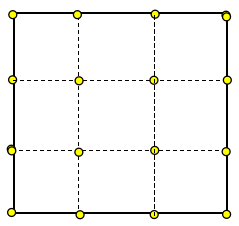
Figure 2: Uniform nodal points on an interior element $K\in\mathcal{T}^{n-1}_{h,I}$.

First we consider each interior element $K\in\mathcal{T}^{n-1}_{h,I}$. Let ${\boldsymbol{A}}^{K}_{ij}$, $0\leq i,j\leq k$, be the nodal points taken uniformly on $K$ (see Fig. 2). Let $P_{k}([0,1])$ be the space of polynomials on $[0,1]$ with degrees $\leq k$ and let $\{b_{0},\cdots,b_{k}\}$ be the basis of $P_{k}([0,1])$ satisfying

$$b_{i}(j/k)=\delta_{i,j},\qquad 0\leq j\leq k,$$

where $\delta_{i,j}$ stands for the Kronecker delta function. An isoparametric transform from the reference element $\hat{K}=[0,1]^{2}$ to $K$ is defined as

$$F_{K}(\boldsymbol{\xi}):=\sum_{i,j=0}^{k}{\boldsymbol{A}}^{K}_{ij}b_{i}(\xi_{1})b_{j}(\xi_{2}),\qquad\forall\,\boldsymbol{\xi}=(\xi_{1},\xi_{2})\in\hat{K}.$$ (15)

We use ${\boldsymbol{X}}^{n-1,n}_{h}$ to trace forward each ${\boldsymbol{A}}^{K}_{ij}$ from $t_{n-1}$ to $t_{n}$ and get the nodal points

$${\boldsymbol{X}}^{n-1,n}_{h}\big{(}{\boldsymbol{A}}^{K}_{ij}\big{)},\qquad 0\leq i,j\leq k.$$

They define another isoparametric transform

$$G_{K}(\boldsymbol{\xi}):=\sum_{i,j=0}^{k}{\boldsymbol{X}}^{n-1,n}_{h}\big{(}{\boldsymbol{A}}^{K}_{ij}\big{)}b_{i}(\xi_{1})b_{j}(\xi_{2})\qquad\forall\,\boldsymbol{\xi}=(\xi_{1},\xi_{2})\in\hat{K}.$$ (16)

We get a homeomorphism from $K$ to $K^{n}:=\big{\{}G_{K}(\boldsymbol{\xi}):\boldsymbol{\xi}\in\hat{K}\big{\}}$

$$\tilde{\boldsymbol{X}}^{n-1,n}_{K}:=G_{K}\circ F_{K}^{-1}.$$ (17)

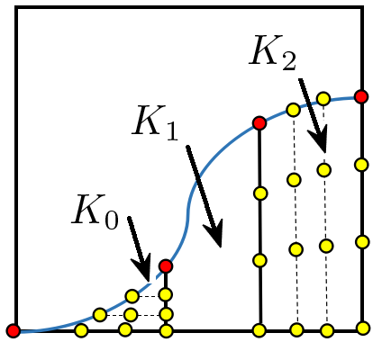
Figure 3: The partition of $K\cap\Omega^{n-1}_{h}$ into curved polygons $K_{0}$, $K_{1}$, and $K_{2}$, where red dots stand for control points in $\mathcal{P}^{n-1}$. Quasi-uniform nodal points are shown on $K_{0}$ and $K_{2}$, respectively.

Next we consider each $K\in\mathcal{T}^{n-1}_{h,B}$. Since $\Gamma^{n-1}_{h}\cap K$ is represented by the piecewise cubic funtion $\boldsymbol{\chi}_{n-1}$. Let $M$ be the number of control points in the interior of $K$. We subdivide $K\cap\bar{\Omega}^{n-1}_{h}$ into $M+1$ curved polygons

$$K\cap\bar{\Omega}^{n-1}_{h}=K_{0}\cup K_{1}\cup\cdots\cup K_{M},\qquad\mathring{K}_{l}\cap\mathring{K}_{m}=\emptyset\quad\hbox{for}\;\;l\neq m.$$

Each $K_{m}$ is either a curved triangle or a curved quadrilateral with only one curved edge $\partial K_{m}\cap\Gamma^{n-1}_{h}$ (see Fig. 3). We define isoparametric transforms for the two cases of $K_{m}$ respectively.

• If $K_{m}$ is a curved quadrilateral (see $K_{2}$ in Fig. 3), we take nodal points ${\boldsymbol{A}}^{K_{m}}_{ij},0\leq i,j\leq k$, quasi-uniformly on $K_{m}$. Similar to (15)–(16), we define two isoparametric transforms as

  $$F_{K_{m}}(\boldsymbol{\xi}):=\sum_{i,j=0}^{k}{\boldsymbol{A}}^{K_{m}}_{ij}b_{i}(\xi_{1})b_{j}(\xi_{2}),\quad G_{K_{m}}(\boldsymbol{\xi}):=\sum_{i,j=0}^{k}{\boldsymbol{X}}^{n-1,n}_{h}\big{(}{\boldsymbol{A}}^{K_{m}}_{ij}\big{)}b_{i}(\xi_{1})b_{j}(\xi_{2}),\quad\forall\,\boldsymbol{\xi}\in\hat{K}.$$ (18)

• If $K_{m}$ is a curved triangle (see $K_{0}$ in Fig. 3), we take $(k+1)(k+2)/2$ nodal points ${\boldsymbol{A}}^{K_{m}}_{ij},0\leq i+j\leq k$, quasi-uniformly on $K_{m}$. Let $\hat{T}$ be the reference triangle with vertices $(0,0)$, $(1,0)$, and $(0,1)$. The two isoparametric transforms are defined as

  $$F_{K_{m}}(\boldsymbol{\xi}):=\sum_{i+j=0}^{k}{\boldsymbol{A}}^{K_{m}}_{ij}b_{ij}(\boldsymbol{\xi}),\quad G_{K_{m}}(\boldsymbol{\xi}):=\sum_{i+j=0}^{k}{\boldsymbol{X}}^{n-1,n}_{h}\big{(}{\boldsymbol{A}}^{K_{m}}_{ij}\big{)}b_{ij}(\boldsymbol{\xi}),\quad\forall\,\boldsymbol{\xi}\in\hat{T},$$ (19)

  where $b_{ij}\in P_{k}(\hat{T})$ satisfies $b_{ij}(l/k,m/k)=\delta_{i,l}\delta_{j,m}$ for two integers satisfying $0\leq l+m\leq k$.

In both cases, they define a homeomorphism from $K_{m}$ to $K^{n}_{m}:=\big{\{}G_{K_{m}}(\boldsymbol{\xi}):\boldsymbol{\xi}\in\hat{K}\big{\}}$

$$\tilde{\boldsymbol{X}}^{n-1,n}_{K_{m}}:=G_{K_{m}}\circ F_{K_{m}}^{-1}.$$ (20)

Therefore, we obtain a homeomorphism $\tilde{\boldsymbol{X}}^{n-1,n}_{K}$: $K\cap\bar{\Omega}^{n-1}_{h}\to K^{n}:=\cup_{m=0}^{M}K^{n}_{m}$

$$\tilde{\boldsymbol{X}}^{n-1,n}_{K}\big{|}_{K_{m}}=\tilde{\boldsymbol{X}}^{n-1,n}_{K_{m}}.$$ (21)

Define $\Omega^{n}_{{\boldsymbol{X}}}:=\cup_{K\in\mathcal{T}^{n-1}_{h}}K^{n}$. Combining (17) and (21), we obtain a homeomorphism $\tilde{\boldsymbol{X}}^{n-1,n}_{h}$: $\bar{\Omega}^{n-1}_{h}\to\bar{\Omega}^{n}_{{\boldsymbol{X}}}$ which is defined piecewise as follows

$$\tilde{\boldsymbol{X}}^{n-1,n}_{h}=\tilde{\boldsymbol{X}}^{n-1,n}_{K}\quad\hbox{on}\;\;K\cap\bar{\Omega}^{n-1}_{h}.$$ (22)

Step 2. Define the backward flow map ${\boldsymbol{X}}^{n,n-1}_{h}$. First we let $\tilde{\boldsymbol{X}}^{n,n-1}_{h}:=\big{(}\tilde{\boldsymbol{X}}^{n,n-1}_{h}\big{)}^{-1}$ which is a homeomorphism from $\bar{\Omega}^{n}_{{\boldsymbol{X}}}$ to $\bar{\Omega}^{n-1}_{h}$. Note that $\tilde{\boldsymbol{X}}^{n,n-1}_{h}$ is undefined on $\Omega^{n}_{h}\backslash\Omega^{n}_{{\boldsymbol{X}}}$. Next we extend it to $\bar{\Omega}^{n}_{h}\cup\bar{\Omega}^{n}_{{\boldsymbol{X}}}$ and denote the extension by the same notation.

For any ${\boldsymbol{x}}\in\partial\Omega^{n}_{{\boldsymbol{X}}}$, let ${\boldsymbol{n}}({\boldsymbol{x}})$ be the unit outer normal at ${\boldsymbol{x}}\in\partial\Omega^{n}_{{\boldsymbol{X}}}$ (see Fig. 4). The extension is defined by constant along ${\boldsymbol{n}}({\boldsymbol{x}})$, namely,

$$\tilde{\boldsymbol{X}}^{n,n-1}_{h}\big{(}{\boldsymbol{x}}+t{\boldsymbol{n}}({\boldsymbol{x}})\big{)}\equiv\tilde{\boldsymbol{X}}^{n,n-1}_{h}({\boldsymbol{x}})\qquad\hbox{for all}\;\;t>0\;\;\hbox{satisfying}\;\;{\boldsymbol{x}}+t{\boldsymbol{n}}_{\boldsymbol{x}}\in\bar{\Omega}^{n}_{h}.$$ (23)

Finally, we define the backward flow map as

$${\boldsymbol{X}}^{n,n-1}_{h}=\tilde{\boldsymbol{X}}^{n,n-1}_{h}\big{|}_{\bar{\Omega}^{n}_{h}}.$$ (24)

Clearly ${\boldsymbol{X}}^{n,n-1}_{h}$: $\bar{\Omega}^{n}_{h}\to\bar{\Omega}^{n-1}_{h}$ is neither surjective nor injective.

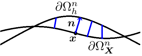
Figure 4: Constant extension of $\tilde{{\boldsymbol{X}}}_{h}^{n,n-1}$ to $\bar{\Omega}^{n}_{h}\backslash\bar{\Omega}^{n}_{{\boldsymbol{X}}}$ along the normal direction ${\boldsymbol{n}}={\boldsymbol{n}}({\boldsymbol{x}})$.

Remark 3.7.

By (15)–(20), the computation of $\tilde{\boldsymbol{X}}^{n-1,n}_{h}=\big{(}\tilde{\boldsymbol{X}}^{n-1,n}_{h}\big{)}^{-1}$ requires two operations

• tracing the nodal points ${\boldsymbol{A}}^{K}_{ij}$, ${\boldsymbol{A}}^{K_{m}}_{ij}$ one step forward $($see (16) and (18)–(19)$)$ ,

• computing composite isoparametric transforms $F_{K}\circ G_{K}^{-1}$ and $F_{K_{m}}\circ G_{K_{m}}^{-1}$ $($see (17) and (20)$)$ .

In view of (24), we know that the computational complexity of ${\boldsymbol{X}}^{n,n-1}_{h}$ is much more economic than that of the inverse map $\big{(}{\boldsymbol{X}}^{n-1,n}_{h}\big{)}^{-1}$. Nevertheless, optimal convergence orders are observed in numerical experiments which use ${\boldsymbol{X}}^{n,n-1}_{h}$.

3.8 Finite element scheme for computing ${\boldsymbol{u}}^{n}_{h}$

Remember that we have obtained the computation domain $\Omega^{n}_{h}$ in subsection 3.3. Let $\mathcal{T}^{n}_{h}$ be the sub-mesh covering $\Omega^{n}_{h}$ and let $\mathcal{E}_{h,B}^{n}$ be the set of boundary-zone edges.

For any edge $E\in\mathcal{E}_{h,B}^{n}$, suppose $E=K_{1}\cap K_{2}$ with $K_{1},K_{2}\in\mathcal{T}_{h}^{n}$. Let ${\boldsymbol{n}}_{K_{1}}$ be the unit normal of $E$ , pointing to the exterior of $K_{1}$, and let ${\boldsymbol{n}}_{K_{2}}=-{\boldsymbol{n}}_{K_{1}}$. The normal jump of a scalar function $v$ across $E$ is defined by

$$\left\llbracket{v}\right\rrbracket({\boldsymbol{x}})=\lim_{\varepsilon\to 0+}\left[v({\boldsymbol{x}}-\varepsilon{\boldsymbol{n}}_{K_{1}}){\boldsymbol{n}}_{K_{1}}+v({\boldsymbol{x}}-\varepsilon{\boldsymbol{n}}_{K_{2}}){\boldsymbol{n}}_{K_{2}}\right]\qquad\forall\,{\boldsymbol{x}}\in E.$$

Clearly $\left\llbracket{{\boldsymbol{v}}}\right\rrbracket$ is a matrix function on $E$ if ${\boldsymbol{v}}$ is a vector function. For two vector functions ${\boldsymbol{v}}$ and ${\boldsymbol{w}}$, the Euclidean inner product of $\left\llbracket{{\boldsymbol{v}}}\right\rrbracket$ and $\left\llbracket{{\boldsymbol{w}}}\right\rrbracket$ is defined by

$$\left\llbracket{{\boldsymbol{v}}}\right\rrbracket:\left\llbracket{{\boldsymbol{w}}}\right\rrbracket=\left\llbracket{v_{1}}\right\rrbracket\cdot\left\llbracket{w_{1}}\right\rrbracket+\left\llbracket{v_{2}}\right\rrbracket\cdot\left\llbracket{w_{2}}\right\rrbracket.$$

Furthermore, we define two bilinear forms on ${\boldsymbol{H}}^{k+1}(\mathcal{T}^{n}_{h})\cap{\boldsymbol{H}}^{1}({D^{n}})$ as follows

$$\mathscr{A}^{n}_{h}({\boldsymbol{w}},{\boldsymbol{v}}):=\, \int_{\Omega^{n}_{h}}\nu\nabla{\boldsymbol{w}}\cdot\nabla{\boldsymbol{v}}+\mathscr{J}_{h}^{n}({\boldsymbol{w}},{\boldsymbol{v}}),$$ (25)

$$\mathscr{J}^{n}_{h}({\boldsymbol{w}},{\boldsymbol{v}}):=\, \gamma\sum_{E\in\mathcal{E}_{h,B}^{n}}\sum_{l=1}^{k}\frac{h^{2l-1}}{[(l-1)!]^{2}}\int_{E}\nu\left\llbracket{\partial_{{\boldsymbol{n}}}^{l}{\boldsymbol{w}}}\right\rrbracket:\left\llbracket{\partial_{{\boldsymbol{n}}}^{l}{\boldsymbol{v}}}\right\rrbracket,$$ (26)

where $\gamma$ is a positive constant whose value will be specified in the section for numerical experiments. Here $\mathscr{J}_{h}^{n}$, called “ghost penalty stabilization” in the literature (cf. [10]), is used to enhance the stability of numerical solutions.

Define $\underline{{\boldsymbol{U}}^{n}_{h}}=\big{[}{\boldsymbol{U}}^{n-k,n}_{h},\cdots,{\boldsymbol{U}}^{n,n}_{h}\big{]}^{\top}$, ${\boldsymbol{U}}^{n,n}_{h}={\boldsymbol{u}}^{n}_{h}$, and ${\boldsymbol{U}}_{h}^{n-i,n}:={\boldsymbol{u}}_{h}^{n-i}\circ{{\boldsymbol{X}}}_{h}^{n,n-i}$ for $1\leq i\leq k$. Similar to (10a), we define the discrete BDF-$k$ difference operator as

$$\frac{1}{\tau}\Lambda^{k}\underline{{\boldsymbol{U}}_{h}^{n}}:=\frac{1}{\tau}\sum_{i=0}^{k}a_{i}^{k}{\boldsymbol{U}}_{h}^{n-i,n}.$$ (27)

The finite element approximation to problem (10) is to seek ${\boldsymbol{u}}^{n}_{h}\in{\boldsymbol{V}}(k,\mathcal{T}_{h}^{n})$ such that $\displaystyle\big{(}\Lambda^{k}\underline{{\boldsymbol{U}}^{n}_{h}},{\boldsymbol{v}}_{h}\big{)}_{\Omega^{n}_{h}}+\tau\mathscr{A}^{n}_{h}({\boldsymbol{u}}_{h}^{n},{\boldsymbol{v}}_{h})=\tau({\boldsymbol{f}}^{n},{\boldsymbol{v}}_{h})_{\Omega^{n}_{h}}\qquad\forall\,{\boldsymbol{v}}_{h}\in{\boldsymbol{V}}(k,\mathcal{T}_{h}^{n}).$ (28)

Remark 3.9.

Suppose that the approximation of $\Gamma^{n}_{h}$ to the exact boundary $\Gamma_{t_{n}}$ is high-order, say

$$\max_{{\boldsymbol{x}}\in\Gamma_{t_{n}}}\min_{{\boldsymbol{y}}\in\Gamma^{n}_{h}}\left|{{\boldsymbol{x}}-{\boldsymbol{y}}}\right|=O(h^{k}),\qquad k\geq 2.$$

From (11) we know that $\bar{\Omega}_{t_{n}}\subset\tilde{\Omega}^{n}_{h}$ if $h$ is small enough. This guarantees that the numerical solution ${\boldsymbol{u}}^{n}_{h}$ is well-defined on the exact domain $\bar{\Omega}_{t_{n}}$. That is why we choose an enlarged domain $\tilde{\Omega}^{n}_{h}\subset D^{n}$ to define the finite element space, instead of the tracked domain $\Omega^{n}_{h}$.

To end this section, we prove the well-posedness of the discrete problem.

Theorem 3.10.

Suppose that the pre-calculated solutions ${\boldsymbol{u}}^{0}_{h},\cdots,{\boldsymbol{u}}^{k-1}_{h}$ are given. Then the discrete problem (28) has a unique solution ${\boldsymbol{u}}^{n}_{h}\in{\boldsymbol{V}}(k,\mathcal{T}^{n}_{h})$ for each $k\leq n\leq N$.

Proof.

From (25) and (26), it is easy to see that the bilinear form $\mathscr{A}^{n}_{h}$ is symmetic and semi-positive on ${\boldsymbol{V}}(k,\mathcal{T}^{n}_{h})$. It suffices to show that $a_{0}^{k}\tau^{-1}({\boldsymbol{v}}_{h},{\boldsymbol{v}}_{h})_{\Omega^{n}_{h}}+\mathscr{A}^{n}_{h}({\boldsymbol{v}}_{h},{\boldsymbol{v}}_{h})=0$ implies ${\boldsymbol{v}}_{h}\equiv 0$. It clearly yields

$${\boldsymbol{v}}_{h}=0\quad\hbox{in}\;\;\Omega^{n}_{h},\qquad\left\llbracket{\partial_{{\boldsymbol{n}}}^{l}{\boldsymbol{v}}_{h}}\right\rrbracket=0\quad\hbox{on any}\;E\in\mathcal{E}^{n}_{h,B},\quad 0\leq l\leq k.$$

The conclusion is obvious. ∎

4 Numerical experiments

In this section, we use three numerical examples to verify the convergence orders of the proposed finite element method. The second and third examples demonstrate the robustness of the method for severely deforming domains.

4.1 An efficient algorithm for computing $\big{(}{\boldsymbol{U}}_{h}^{n,n-i},{\boldsymbol{v}}_{h}\big{)}_{\Omega_{h}^{n}}$

Remember from (28) that we need to calculate the integrals accurately and efficiently

$$\big{(}{\boldsymbol{U}}_{h}^{n,n-i},{\boldsymbol{v}}_{h}\big{)}_{\Omega^{n}_{h}}=\big{(}{\boldsymbol{u}}_{h}^{n-i}\circ{\boldsymbol{X}}^{n,n-i}_{h},{\boldsymbol{v}}_{h}\big{)}_{\Omega^{n}_{h}}\quad\hbox{for}\;\;1\leq i\leq k\;\;\hbox{and}\;\;{\boldsymbol{v}}_{h}\in{\boldsymbol{V}}(k,\mathcal{T}^{n}_{h}).$$

For $i\geq 2$, the computation of $\big{(}{\boldsymbol{u}}_{h}^{n-i}\circ{\boldsymbol{X}}^{n,n-i}_{h},{\boldsymbol{v}}_{h}\big{)}_{\Omega^{n}_{h}}$ involves multi-step map ${\boldsymbol{X}}^{n,n-i}_{h}$ and is time-consuming. To simplify the computation while keep accuracy, we make the replacement in calculating the integral

$$\big{(}{\boldsymbol{U}}_{h}^{n,n-i},{\boldsymbol{v}}_{h}\big{)}_{\Omega^{n}_{h}}\approx\big{(}\hat{\boldsymbol{u}}_{h}^{n,n-i},{\boldsymbol{v}}_{h}\big{)}_{\Omega^{n}_{h}},$$

where $\hat{\boldsymbol{u}}_{h}^{n,n-i}\in{\boldsymbol{V}}(k,\mathcal{T}_{h}^{n})$ is defined in Algorithm 4.2 via modified $L^{2}$-projections. The computation of $\hat{\boldsymbol{u}}_{h}^{n,n-i}$ only involves one-step maps and reduces the computational time significantly.

Algorithm 4.2.

The functions $\hat{\boldsymbol{u}}_{h}^{n,n-i}\in{\boldsymbol{V}}(k,\mathcal{T}_{h}^{n})$, $1\leq i\leq k$, are calculated successively. Suppose that $\hat{\boldsymbol{u}}_{h}^{n-1,n-i}\in{\boldsymbol{V}}(k,\mathcal{T}_{h}^{n-1})$, $2\leq i\leq k$, have been obtained. Find $\hat{\boldsymbol{u}}_{h}^{n,n-i}\in{\boldsymbol{V}}(k,\mathcal{T}_{h}^{n})$ such that

$$\mathscr{M}^{n}_{h}\big{(}\hat{\boldsymbol{u}}_{h}^{n,n-i},{\boldsymbol{v}}_{h}\big{)}=(\hat{{\boldsymbol{u}}}_{h}^{n-1,n-i}\circ{{\boldsymbol{X}}}_{h}^{n,n-1},{\boldsymbol{v}}_{h})_{\Omega_{h}^{n}}\quad\forall\,{\boldsymbol{v}}_{h}\in{\boldsymbol{V}}(k,\mathcal{T}_{h}^{n}),\quad 1\leq i\leq k.$$ (29)

where $\hat{{\boldsymbol{u}}}_{h}^{n-1,n-1}={\boldsymbol{u}}^{n-1}_{h}$ and

$$\mathscr{M}^{n}_{h}({\boldsymbol{w}},{\boldsymbol{v}}):=\, \int_{\Omega^{n}_{h}}{\boldsymbol{w}}\cdot{\boldsymbol{v}}+\gamma\sum_{E\in\mathcal{E}_{h,B}^{n}}\sum_{l=1}^{k}\frac{h^{2l+1}}{(l!)^{2}}\int_{E}\left\llbracket{\partial_{{\boldsymbol{n}}}^{l}{\boldsymbol{w}}}\right\rrbracket:\left\llbracket{\partial_{{\boldsymbol{n}}}^{l}{\boldsymbol{v}}}\right\rrbracket.$$

4.3 The computation of $\big{(}{\boldsymbol{w}}_{h}\circ{\boldsymbol{X}}_{h}^{n,n-1},{\boldsymbol{v}}_{h}\big{)}_{\Omega_{h}^{n}}$ for any ${\boldsymbol{w}}_{h}\in{\boldsymbol{V}}(k,\mathcal{T}_{h}^{n-1})$ and ${\boldsymbol{v}}_{h}\in{\boldsymbol{V}}(k,\mathcal{T}_{h}^{n})$

Using (24), we approximate the integral as follows

$$\big{(}{\boldsymbol{w}}_{h}\circ{{\boldsymbol{X}}}_{h}^{n,n-1},{\boldsymbol{v}}_{h}\big{)}_{\Omega^{n}_{h}}=\big{(}{\boldsymbol{w}}_{h}\circ\tilde{{\boldsymbol{X}}}_{h}^{n,n-1},{\boldsymbol{v}}_{h}\big{)}_{\Omega^{n}_{h}}\approx\big{(}{\boldsymbol{w}}_{h}\circ\tilde{{\boldsymbol{X}}}_{h}^{n,n-1},{\boldsymbol{v}}_{h}\big{)}_{\Omega^{n}_{\boldsymbol{X}}}=\big{(}{\boldsymbol{w}}_{h}\circ\big{(}\tilde{{\boldsymbol{X}}}_{h}^{n-1,n}\big{)}^{-1},{\boldsymbol{v}}_{h}\big{)}_{\Omega^{n}_{\boldsymbol{X}}},$$

where $\Omega^{n}_{\boldsymbol{X}}=\tilde{\boldsymbol{X}}^{n-1,n}_{h}(\Omega^{n-1}_{h})$. By (22), $\tilde{\boldsymbol{X}}^{n-1,n}_{h}$ is a homeomorphism from $\bar{\Omega}^{n-1}_{h}$ to $\Omega^{n}_{\boldsymbol{X}}$ and provides an approximation to the forward flow map ${\boldsymbol{X}}^{n-1,n}_{h}$. Moreover, $\tilde{\boldsymbol{X}}^{n-1,n}_{h}$ is defined piecewise on each $K\in\mathcal{T}^{n-1}_{h}$. By (15)–(20), the integral on the right-hand side can be calculated as follows

$$\big{(}{\boldsymbol{w}}_{h}\circ\big{(}\tilde{{\boldsymbol{X}}}_{h}^{n-1,n}\big{)}^{-1},{\boldsymbol{v}}_{h}\big{)}_{\Omega^{n}_{\boldsymbol{X}}}=\, \sum_{K\in\mathcal{T}^{n-1}_{h,I}}\int_{\hat{K}}({\boldsymbol{w}}_{h}\circ F_{K})\cdot({\boldsymbol{v}}_{h}\circ G_{K})\left|{\det(\mathrm{d}_{\boldsymbol{\xi}}G_{K})}\right|$$

$$+\sum_{K\in\mathcal{T}^{n-1}_{h,B}}\sum_{m=0}^{M}\int_{\hat{K}_{m}}({\boldsymbol{w}}_{h}\circ F_{K_{m}})\cdot({\boldsymbol{v}}_{h}\circ G_{K_{m}})\left|{\det(\mathrm{d}_{\boldsymbol{\xi}}G_{K_{m}})}\right|,$$ (30)

where $\hat{K}_{m}=\hat{K}$ if $K_{m}$ is a curved quadriliteral and $\hat{K}_{m}=\hat{T}$ if $K_{m}$ is a curved triangle (see subsection 3.6). Here $F_{K}$ is the isoparametric transform from the reference element $\hat{K}$ to $K$ or $K_{m}$, $G_{K}$ is the isoparametric transform from $\hat{K}$ to $K^{n}$ or $K^{n}_{m}$, and $\mathrm{d}_{\boldsymbol{\xi}}G_{K}$, $\mathrm{d}_{\boldsymbol{\xi}}G_{K_{m}}$ are Jacobi matrices of $G_{K}$ and $G_{K_{m}}$, respectively. Each integral on reference elements will be computed with Gaussian quadrature rule of the $(k+1)^{\rm th}$-order.

Since $\hat{{\boldsymbol{u}}}_{h}^{n-1,n-i}\in{\boldsymbol{V}}(k,\mathcal{T}^{n-1}_{h})$, the right-hand side of (29) can be calculated with the formula (30).

4.4 Numerical examples

In this section, we report three examples for various scenarios of the domain: rotation, vortex shear, and severe deformation. In order to test convergence orders of the method, we take ${\boldsymbol{u}}$ as smooth functions and set the right-hand side of (1) by

$${\boldsymbol{f}}=\partial_{t}{\boldsymbol{u}}+{\boldsymbol{u}}\cdot\nabla{\boldsymbol{u}}-\nu\Delta{\boldsymbol{u}}.$$

The Neumann condition is set by

$${\boldsymbol{g}}_{N}:=\nabla{\boldsymbol{u}}\cdot{\boldsymbol{n}}\quad\hbox{on}\;\;\Gamma_{t}.$$

For each example, we require that the final shape of domain $\Omega_{T}$ coincides with the initial shape $\Omega_{0}$. This helps us to compute the surface-tracking error

$$e_{\Omega}=\sum_{K\in\mathcal{T}_{h}}\left|\mathrm{area}\big{(}\Omega_{T}\cap K\big{)}-\mathrm{area}\big{(}\Omega^{N}_{h}\cap K\big{)}\right|,$$ (31)

which is also called the geometrical error [1, 2]. Here $t_{N}=T$ is the final time of evolution. Since the exact boundary $\Gamma_{T}$ and the approximate boundary $\Gamma^{N}_{h}$ are very close, calculating the exact area of domain difference directly

$$e_{0,\Omega}=\mathrm{area}(\Omega_{T}\backslash\Omega_{h}^{N})+\mathrm{area}(\Omega_{h}^{N}\backslash\Omega_{T})$$

may cause an ill-conditioned problem. In fact, it is easy to see that $e_{\Omega}\to e_{0,\Omega}$ as $h\to 0$.

To measure the error between the exact velocity and the numerical solution, we use

$$e_{0}=\left\|{{\boldsymbol{u}}(\cdot,T)-{\boldsymbol{u}}_{h}^{N}}\right\|_{{\boldsymbol{L}}^{2}(\Omega_{T})},$$

since $\Omega_{T}=\Omega_{0}$ is explicitly given. However, $\Omega_{t_{n}}$ are unknown in intermediate time steps. We measure the $H^{1}$-norm errors on the computational domains by

$$e_{1}=\bigg{(}\sum_{n=k}^{N}\tau\left|{{\boldsymbol{u}}(\cdot,t_{n})-{\boldsymbol{u}}_{h}^{n}}\right|_{{\boldsymbol{H}}^{1}(\Omega_{h}^{n})}^{2}\bigg{)}^{1/2}.$$

Throughout this section, we set the diffusion coefficient by $\nu=1$. Other constant values of $\nu$ do not influence the convergence orders for $\tau$ small enough. The penalty parameter is set by $\gamma=0.001$ in $\mathscr{J}^{n}_{h}$. In Algorithm 3.4, the parameters for surface-tracking are set by $\eta=0.5h$ and $\delta=0.01$.

Example 4.5 (Rotation of an elliptic disk).

The exact velocity is set by

$${\boldsymbol{u}}=(0.5-y,x-0.5).$$

The initial domain is an elliptic disk whose center is located at $(0.5,0.5)$, major axis $R_{1}=0.6$, and minor axis $R_{2}=0.3$. The finial time is set by $T=\pi$.

The moving domain $\Omega_{t}$ rotates half a circle counterclockwise with angular velocity $=1$ and returns to its original shape at $t=T$. Fig. 8 shows the snapshots of $\Omega^{n}_{h}$ which are formed with Algorithm 3.4 at $t_{n}=0$, $T/8$, $T/4$, $T/2$, $3T/4$, and $T$, respectively. From Tables 6 and 7, we find that optimal convergence orders are obtained for both the SBDF-3 and SBDF-4 schemes, namely,

$$e_{0}\sim\tau^{k},\qquad e_{1}\sim\tau^{k},\qquad e_{\Omega}\sim\tau^{k},\qquad k=3,4.$$

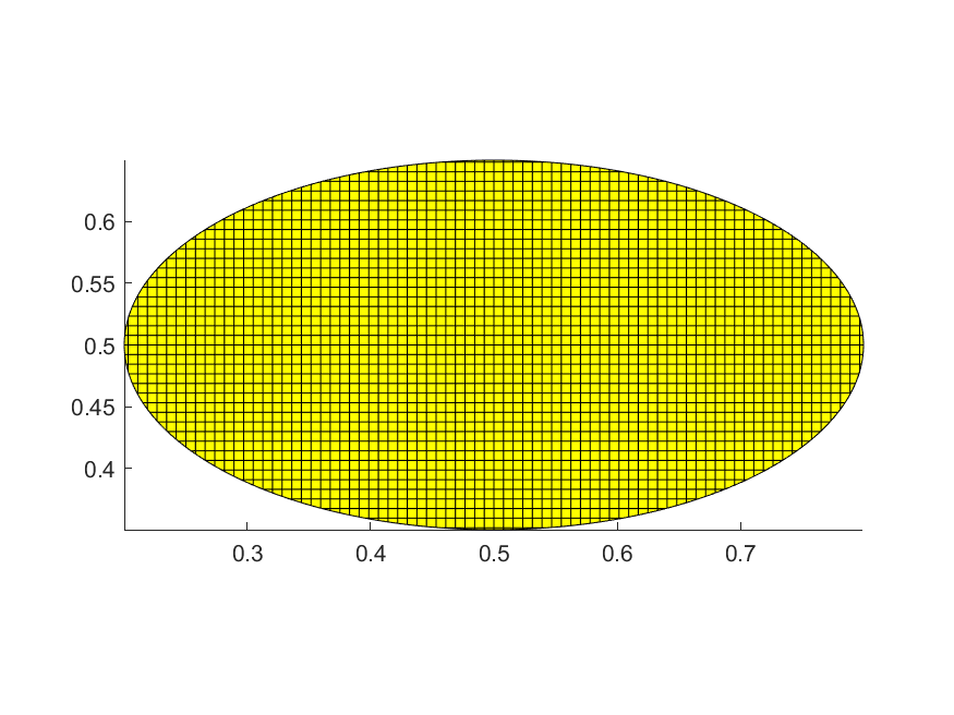
(a) $t=0$

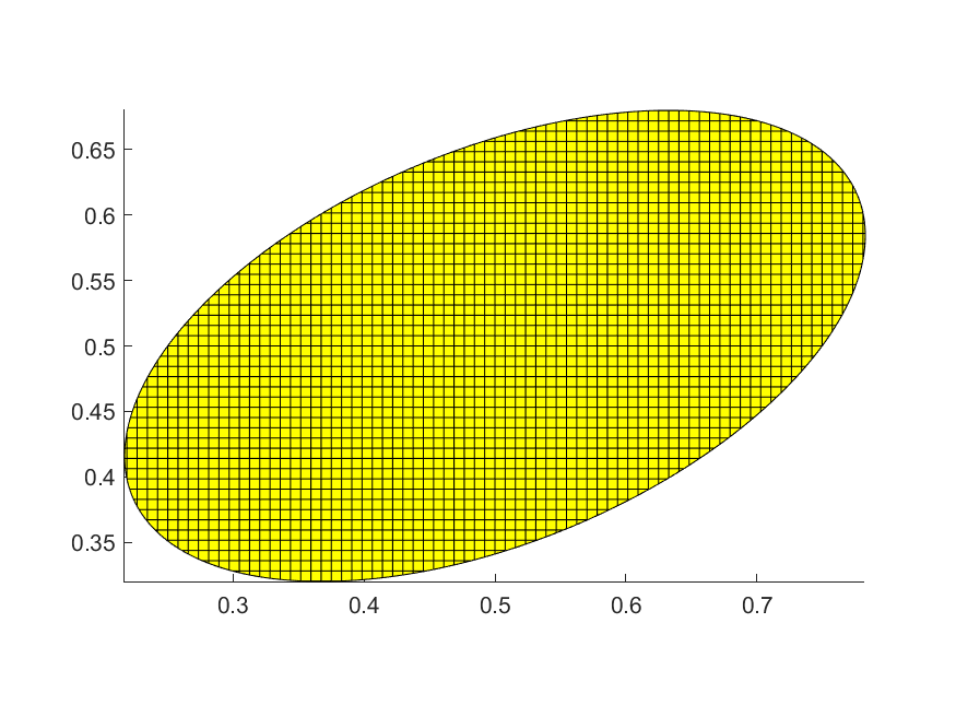
(b) $t=T/8$

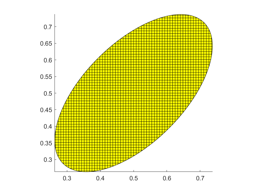
(c) $t=T/4$

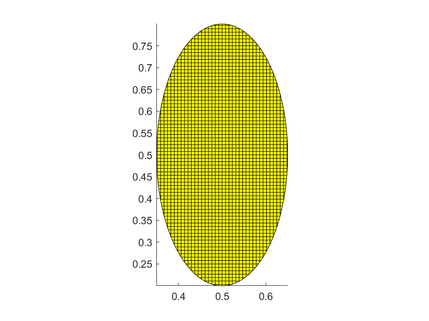
(d) $t=T/2$

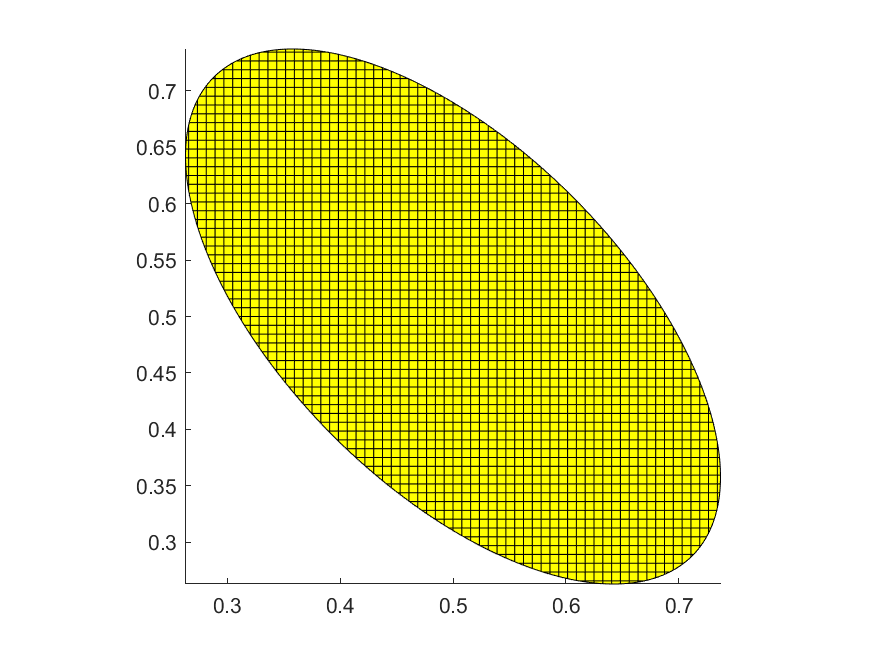
(e) $t=3T/4$

(f) t=$T$

Figure 5: Computational domains $\Omega^{n}_{h}$ at different time steps $(h=1/128,\;k=3)$.

Table 2: Convergence orders for the SBDF-3 scheme (Example 4.5).

$h=\tau/\pi$	$e_{0}$	Order	$e_{1}$	Order	$e_{\Omega}$	Order
1/16	1.06e-05	-	1.10e-04	-	4.03e-03	-
1/32	1.36e-06	2.93	1.47e-05	2.91	5.73e-04	2.81
1/64	1.71e-07	2.99	1.89e-06	2.96	7.54e-05	2.92
1/128	2.14e-08	3.00	2.39e-07	2.98	9.64e-06	2.97

Table 3: Convergence orders for the SBDF-4 scheme (Example 4.5).

$h=\tau/\pi$	$e_{0}$	Order	$e_{1}$	Order	$e_{\Omega}$	Order
1/16	2.13e-06	-	2.17e-05	-	4.14e-04	-
1/32	1.34e-07	3.98	1.44e-06	3.91	2.83e-05	3.87
1/64	8.42e-09	4.00	9.26e-08	3.96	1.86e-06	3.93
1/128	5.56e-10	3.92	5.88e-09	3.98	1.20e-07	3.96

Example 4.6 (Vortex shear of a circular disk).

The exact velocity is given by

$${\boldsymbol{u}}=\cos(\pi t/3)\big{(}\sin^{2}(\pi x)\sin(2\pi y),\,-\sin^{2}(\pi y)\sin(2\pi x)\big{)}.$$

The initial domain is a disk with radius $R=0.15$ and centering at $(0.5,0.75)$. The final time is $T=3$.

The domain is stretched into a snake-like region at $T/2$ and goes back to its initial shape at $t=T$. Fig. 6 shows the snapshots of the computational domain $\Omega^{n}_{h}$ during the time evolution procedure. Tables 2 and 3 show optimal convergence orders for both the SBDF-3 and SBDF-4 schemes, respectively. From Fig. 6 (d), we find that although the domain experiences severe deformations, high-order convergence is still obtained. This demonstrates the robustness of the finite element method.

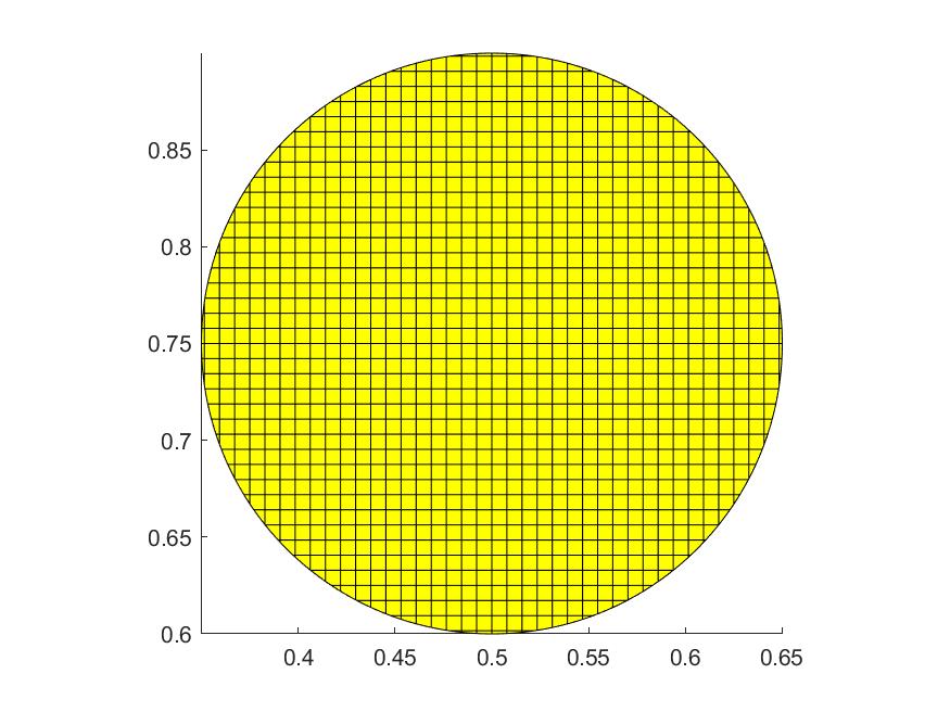
(a) t=$0$

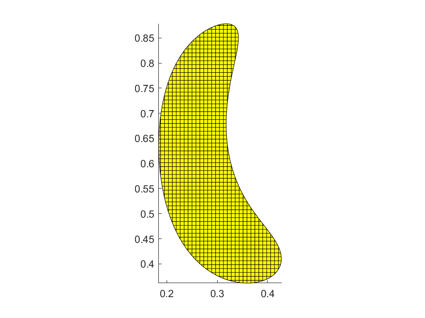
(b) $t=T/8$

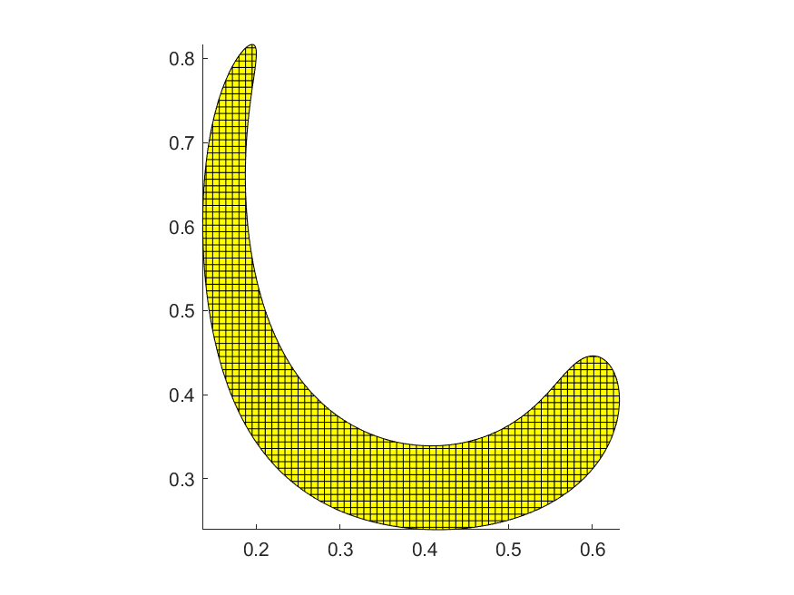
(c) $t=T/4$

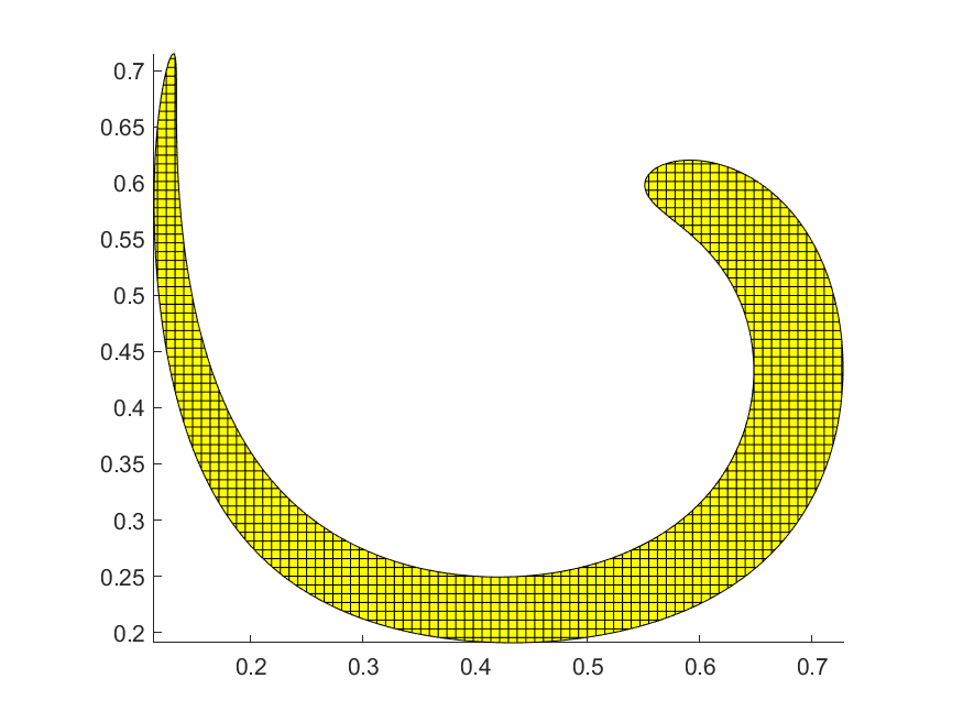
(d) $t=T/2$

(e) $t=3T/4$

(f) $t=T$

Figure 6: Computational domains $\Omega^{n}_{h}$ at different time steps $(h=1/128,\;k=3)$.

Table 4: Convergence orders for the SBDF-3 scheme (Example 4.6).

$h=\tau$	$e_{0}$	Order	$e_{1}$	Order	$e_{\Omega}$	Order
1/16	1.17e-03	-	1.71e-03	-	6.70e-03	-
1/32	1.07e-04	3.45	2.00e-04	3.09	1.03e-03	2.71
1/64	9.59e-06	3.48	2.51e-05	3.00	1.45e-04	2.82
1/128	9.52e-07	3.33	3.16e-06	2.99	1.89e-05	2.94

Table 5: Convergence orders for the SBDF-4 scheme (Example 4.6).

$h=\tau$	$e_{0}$	Order	$e_{1}$	Order	$e_{\Omega}$	Order
1/16	1.60e-03	-	7.40e-04	-	1.14e-02	-
1/32	1.18e-04	3.76	5.80e-05	3.67	7.20e-04	3.98
1/64	7.62e-06	3.95	3.95e-06	3.87	4.24e-05	4.08
1/128	4.78e-07	3.99	2.53e-07	3.97	2.51e-06	4.08

Example 4.7 (Deformation of a circular disk).

The exact solution is given by

$${\boldsymbol{u}}=\cos(\pi t/3)\big{(}\sin(2\pi x)\sin(2\pi y),\cos(2\pi x)\cos(2\pi y)\big{)}.$$

The initial domain $\Omega_{0}$ is same to that in Example 4.6, that is, a disk of radius $R=0.15$ and centering at $(0.5,0.5)$. The final time is set by $T=3$.

In this example, the deformation of the domain is even more severe than that in Example 4.6. At $t=T/2$, the middle part of the domain is stretched into a filament (see Fig. 7). At this time, the domain attains its largest deformation compared with the initial shape. In the second half period, the domain returns to its initial shape. Moreover, we adopt a fine mesh with $h=1/256$ to capture the largest deformation of the domain. Nevertheless, Tables 4 and 5 show that quasi-optimal convergence is observed for both the SBDF-3 and SBDF-4 schemes, respectively. This indicates that

$$e_{0}\sim\tau^{k},\qquad e_{1}\sim\tau^{k},\qquad e_{\Omega}\sim\tau^{k},\qquad k=3,4,$$

hold asymptotically as $\tau=h\to 0$.

Finally, Fig. 6 shows the computational domains formed with the surface-tracking Algorithm 3.4 during the time evolution procedure. The severe deformations demonstrate the competitive behavior of the finite element method.

Table 6: Convergence orders for the SBDF-3 scheme (Example 4.7).

$h=\tau$	$e_{0}$	Order	$e_{1}$	Order	$e_{\Omega}$	Order
1/32	9.41e-05	-	5.13e-04	-	7.56e-03	-
1/64	3.88e-06	4.60	6.13e-05	3.06	1.01e-03	2.90
1/128	3.49e-07	3.47	7.85e-06	2.96	1.28e-04	2.98
1/256	5.25e-08	2.73	9.95e-07	2.98	1.60e-05	3.00

Table 7: Convergence orders for the SBDF-4 scheme (Example 4.7).

$h=\tau$	$e_{0}$	Order	$e_{1}$	Order	$e_{\Omega}$	Order
1/32	9.77e-05	-	2.65e-04	-	2.57e-04	-
1/64	9.03e-06	3.44	1.27e-05	4.38	6.83e-05	1.91
1/128	6.04e-07	3.90	7.77e-07	4.03	6.39e-06	3.42
1/256	3.84e-08	3.98	5.12e-08	3.92	4.82e-07	3.73

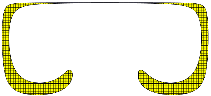
Figure 7: The computational domain $\Omega^{n}_{h}$ at $t_{n}=T/2$ $(h=1/128,\;k=4)$.

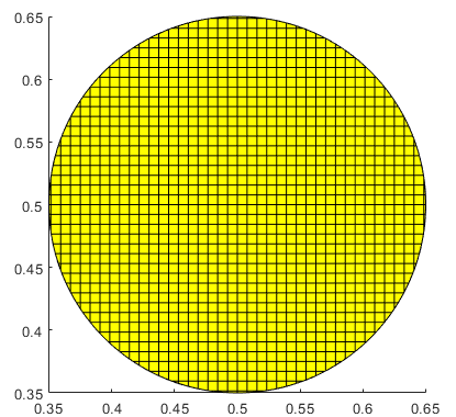
(a) $t=0$

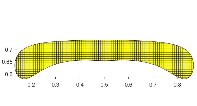
(b) $t=T/8$

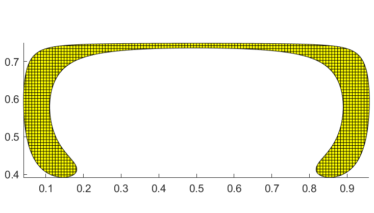
(c) $t=T/4$

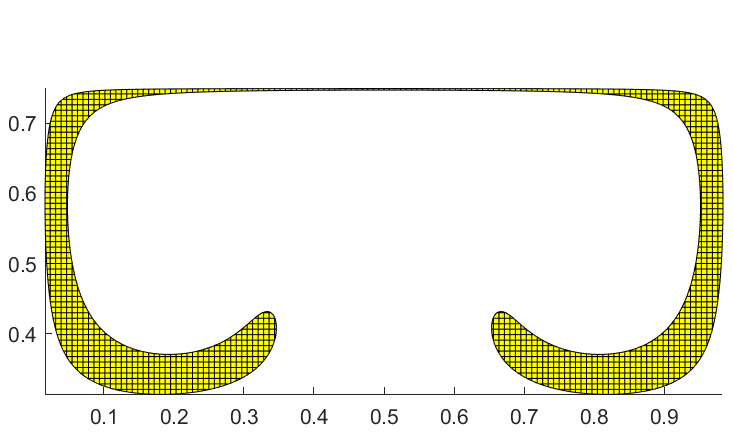
(d) $t=T/2$

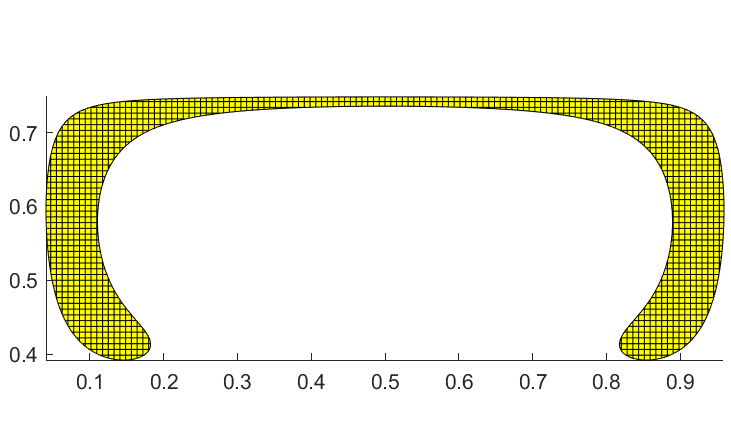
(e) $t=3T/4$

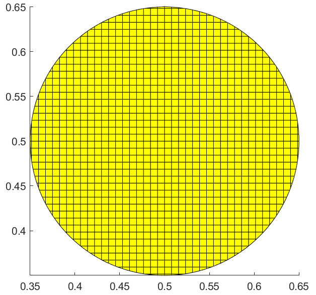
(f) $t=T$

Figure 8: Computational domains $\Omega^{n}_{h}$ at different time steps $(h=1/128,\;k=4)$.

References

• [1] E. Aulisa, S. Manservisi, R. Scardovelli, A mixed markers and volume-of-fluid method for the reconstruction and advection of interfaces in two-phase and free-boundary flows, J. Comput. Phys., 188 (2003), pp. 611–639.
• [2] E. Aulisa, S. Manservisi, R. Scardovelli, A surface marker algorithm coupled to an area-preserving marker redistribution method for three-dimensional interface tracking, J. Comput. Phys., 197 (2004), pp. 555–584.
• [3] H.T. Ahn and M. Shashkov, Multi-material interface reconstruction on generalized polyhedral meshes, J. Comput. Phys., 226 (2007), pp. 2096–2132.
• [4] H.T. Ahn and M. Shashkov, Adaptive moment-of-fluid method, J. Comput. Phys., 228 (2009), pp. 2792–2821.
• [5] A. Alex, Level Set Methods and Fast Marching Methods: Evolving Interfaces in Computational Geometry, Fluid Mechanics, Computer Vision, and Materials Science, Cambridge University Press, 1999.
• [6] U. M. Ascher, S.J. Ruuth and B. T. R. Wetton, Implicit-Explicit methods for time-dependent partial differential equations, SIAM J. Sci. Comput., 32 (1995), pp. 797–823.
• [7] R. Becker, E. Burman and P. Hansbo, A Nitsche extended finite element method for incompressible elasticity with discontinuous modulus of elasticity, Comput. Methods Appl. Mech. Engrg., 198 (2009), pp. 3352–3360.
• [8] W.P. Breugem, A second-order accurate immersed boundary method for fully resolved simulations of particle-laden flows, J. Comput. Phys., 231 (2012), pp. 4469–4498.
• [9] E. Burman and P. Hansbo, Fictitious domain finite element methods using cut elements: I. A stabilized Lagrange multiplier method, Comput. Methods Appl. Mech. Engrg., 199 (2010), pp. 2680–2686.
• [10] E. Burman and P. Hansbo, Interior-penalty stabilized Lagrange multiplier methods for the finite-element solution of elliptic interface problems, IMA J. Numer. Anal., 30 (2010), pp. 870–885.
• [11] E. Burman and P. Hansbo, Fictitious domain finite element methods using cut elements: II. A stabilized Nitsche method, Appl. Numer. Math., 62 (2012), pp. 328–341.
• [12] V. Dyadechko and M. Shashkov, Reconstruction of multi-material interfaces from moment data, J. Comput. Phys., 227 (2008), pp. 5361–5384.
• [13] Y. Giga, Surface Evolution Equations: A Level Set Approach, Monogr. Math. 99, Birkh$\ddot{\rm a}$user, Basel, 2006.
• [14] R. Guo, Solving parabolic moving interface problems with dynamical immersed spaces on unfitted meshes:fully discrete analysis, SIAM J. Numer. Anal., 59 (2021), pp. 797–828.
• [15] A. Hansbo and P. Hansbo, An unfitted finite element method, based on Nitsche’s method, for elliptic interface problems, Comput. Methods Appl. Mech. Engrg., 191 (2002), pp. 5537–5552.
• [16] D. J. E. Harvie and D. F. Fletcher, A new volume of fluid advection algorithm: The stream scheme, J. Comput. Phys., 162 (2000), pp. 1–32.
• [17] M. Herrmann, A balanced force refined level set grid method for two-phase flows on unstructured flow solver grids, J. Comput. Phys., 227 (2008), pp. 2674–2706.
• [18] C. W. Hirt and B. D. Nichols, Volume of fluid (VOF) method for the dynamics of free boundaries, J. Comput. Phys., 39 (1981), pp. 201–225.
• [19] P. Huang, H. Wu, and Y. Xiao, An unfitted interface penalty finite element method for elliptic interface problems, Comput. Methods Appl. Mech. Engrg., 323 (2017) pp. 439–460.
• [20] H. Jaroslav and R. Yves, A new fictitious domain approach inspired by the extended finite element method, SIAM J.Numer. Anal. 47 (2009), pp. 1474–1499.
• [21] R. Kumara, L. Cheng, Y. Xiong, B. Xie, R. Abgrall, and F. Xiao, THINC scaling method that bridges VOF and level set schemes, J. Comput. Phys., 436 (2021), 110323.
• [22] C. Lehrenfeld, The Nitsche XFEM-DG space-time method and its implementation in three space dimensions, SIAM J. Sci. Comput., 37 (2015), pp. A245–A270.
• [23] C. Lehrenfeld and R. Arnold, Analysis of a Nitsche XFEM-DG discretization for a class of two-phase mass transport problems, SIAM J.Numer. Anal. 51 (2013), pp. 958–983.
• [24] R.J. LeVeque and Z. Li, The immersed interface method for elliptic equations with discontinuous coefficients and singular sources, SIAM J. Numer. Anal., 31 (1994), pp. 1019–1044.
• [25] Z. Li and K. Ito, The Immersed Interface Method: Numerical Solutions of PDEs Involving Interfaces and Irregular Domains, Frontiers in Applied Mathematics, Society for Industrial and Applied Mathematics, 2006.
• [26] Z. Li, The immersed interface method using a finite element formulation, Appl. Numer. Math., 27 (1998), pp. 253–267.
• [27] Z. Li, T. Lin, and X. Wu, New Cartesian grid methods for interface problems using the finite element formulation, Numer. Math., 96 (2003), pp. 61–98.
• [28] T. Lin, Y. Lin and X. Zhang, Partially penalized immersed finite element methods for elliptic interface problems, SIAM J.Numer. Anal. 79 (2009), pp. 69–93.
• [29] H. Liu, L. Zhang, X. Zhang, and W. Zheng, Interface-penalty finite element methods for interface problems in $H^{1}$, ${\boldsymbol{H}}(\operatorname{{\bf curl}})$, and ${\boldsymbol{H}}(\operatorname{div})$, Comput. Methods Appl. Mech. Engrg., 367 (2020), 113137.
• [30] J. Liu, Simple and efficient ALE methods with provable temporal accuracy up to fifth order for the Stokes equations on time-varying domains, SIAM J. Numer. Anal., 51 (2013), pp. 743–772.
• [31] C. Ma, Q. Zhang, and W. Zheng, A high-order fictitious-domain method for the advection-diffusion equation on time-varying domain, arXiv:2104.01870 .
• [32] A. Massing, M.G. Larson, A. Logg, and M.E. Rognes, A stabilized Nitsche fictitious domain method for the Stokes problem, J. Sci. Comput., 61 (2014), pp. 604–628.
• [33] R. Mittal and G. Iaccarino, Immersed boundary methods, Ann. Rev. Fluid Mech., 37 (2005), pp. 239–261.
• [34] N.R. Morgan and J.I. Waltz, 3D level set methods for evolving fronts on tetrahedral meshes with adaptive mesh refinement, J. Comput. Phys., 336 (2017), pp. 492–512.
• [35] S. Osher and J.A. Sethian, Fronts Propagating with Curvature Dependent Speed: Algorithms Based on Hamilton-Jacobi Formulations, J. Comput. Phys., 79 (1988), pp. 12–49.
• [36] S. Osher and R.P. Fedkiw, Level Set Methods: An Overview and Some Recent Results, J. Comput. Phys., 169 (2000), pp. 463–502.
• [37] C. S. Peskin, Numerical analysis of blood flow in the heart, J. Comput. Phys., 25 (1977), pp. 220–252.
• [38] G. Tryggvason, B. Bunner, D. Juric, W. Tauber, S. Nas, J. Han, N. Al-Rawahi, and Y.-J. Jan, A front-tracking method for the computations of multiphase flow, J. Comput. Phys., 169 (2001), pp. 708–759.
• [39] H. Wu and Y. Xiao, An unfitted hp-interface penalty finite element method for elliptic interface problems, J. Comp. Math., 37 (2019), pp. 316–339.
• [40] Q. Zhang and A. Fogelson, Fourth-order interface tracking in two dimensions via an improved polygonal area mapping method, SIAM J. Sci. Comput., 36 (2014), pp. A2369–A2400.
• [41] Q. Zhang and A. Fogelson, Mars: An analytic framework of interface tracking via mapping and adjusting regular semialgebraic sets, SIAM J. Numer. Anal., 54 (2016), pp. 530–560.
• [42] Q. Zhang, HFES: A height function method with explicit input and signed output for high-order estimations of curvature and unit vectors of planar curves, SIAM J.Numer. Anal., 55 (2017), pp. 1024–1056.
• [43] Q. Zhang and A. Fogelson, Fourth-and higher-order interface tracking via mapping and adjusting regular semianalytic sets represented by cubic splines, SIAM J. Sci. Comput., 40 (2018), pp. A3755–A3788.
• [44] P. Zhao and J.C. Heinrich, Front-tracking finite element method for dendritic solidification, J. Comput. Phys., 173 (2001), pp. 765–796.