What Can Linear Interpolation of Neural Network Loss Landscapes Tell Us?

Abstract

Studying neural network loss landscapes provides insights into the nature of the underlying optimization problems. Unfortunately, loss landscapes are notoriously difficult to visualize in a human-comprehensible fashion. One common way to address this problem is to plot linear slices of the landscape, for example from the initial state of the network to the final state after optimization. On the basis of this analysis, prior work has drawn broader conclusions about the difficulty of the optimization problem. In this paper, we put inferences of this kind to the test, systematically evaluating how linear interpolation and final performance vary when altering the data, choice of initialization, and other optimizer and architecture design choices. Further, we use linear interpolation to study the role played by individual layers and substructures of the network. We find that certain layers are more sensitive to the choice of initialization, but that the shape of the linear path is not indicative of the changes in test accuracy of the model. Our results cast doubt on the broader intuition that the presence or absence of barriers when interpolating necessarily relates to the success of optimization.

1 Introduction

Neural network loss landscapes are difficult to visualize due to their high-dimensionality and the complicated nature of the actual optimization path. This motivated the use of the loss along the linear path between the initial and final parameters of a neural network as a crude yet simple measure of the loss landscape (Goodfellow et al., 2015). In this work we revisit this 1D linear interpolation technique and address whether the shape of the path reflects the test accuracy of the model and can inform training.

Linear interpolation from beginning to end. Goodfellow et al. (2015) observed that for fully-connected and convolutional networks with maxout (Goodfellow et al., 2013) trained on MNIST data the loss decays monotonically along the linear path between their initial and final state. The absence of obstacles along the linear path led them to conclude that “these tasks are relatively easy to optimize.” This result has been cited widely as an indication of the ease of training (e.g., Li et al. (2018a); McCandlish et al. (2018); Fort et al. (2019)) and the linear interpolation technique itself was used in many papers (Huang et al., 2017; Keskar et al., 2017; Izmailov et al., 2018; Jastrzȩbski et al., 2018; Hao et al., 2019). In this paper we address empirically how meaningful the use of this linear path actually is. The exact definition of training tasks being “easy to optimize” is an open question and optimization choices directly influence which linear path we observe. It is also arguable whether we actually want tasks to be easier to optimize; lowering the amount of training data or reducing regularization simplifies training but lowers test accuracy.

The work by Goodfellow et al. (2015) was recently revisited and extended by Frankle (2020) and Lucas et al. (2021) for a range of modern neural network models, such as ResNet and VGG architectures, on image data sets. Frankle (2020) observed for default parameter settings that the loss often remained at the level of random chance until close to the optimum for these models, different than the behavior observed by Goodfellow et al. (2015). In addition to concurrently confirming this result, Lucas et al. (2021) found that the monotonic decay property observed by Goodfellow et al. (2015) was often maintained when BatchNorm was removed and non-adaptive optimizers were used. On this basis, they hypothesized that “large distances moved in weight space encourage non-monotonic interpolation.”

In our work, we interrogate conjectures stated in prior work that the shape of loss along the linear path relates to the “success” of optimization (which we measure in terms of test accuracy) or other aspects of optimization (e.g., distance travelled). We systematically study the influence of various optimizer and architecture design choices on the shape of the linear path and the test accuracy of the final model, and examine interpolation for individual layers in addition to the entire network. An overview of our results is shown in Table 1. Our main finding is that there are situations that both support and violate the aforementioned intuitions on the shape of the linear path. As such, we recommend caution when using this analysis to infer other information about the nature of the optimization problem.

Table 1: The effect of various interventions in training in (1) the shape of loss over the linear path between the initial and final state of the network and (2) the final test accuracy of the network. Different shapes of loss over the linear path are: no barrier (NB), barrier (B), and plateau (P). If the height of layer-wise barriers changes, we denote this as H-LB (higher) and L-LB (lower layer-wise barriers).

Category	Intervention	Shape of the linear path	Test accuracy
	Pre-train full model (Fig. 2A)	NB	Better
Initialization	Pre-train on random labels (Fig. 2B)	H-LB	Worse (if no weight decay)
(Sec. 4)	Height of the barrier initialization (Fig. 3)	NB	Better
	Partial (pre-)training (Fig. 4)	B/NB/P	Often worse
	Partial random label pre-training (Fig. 5)	B/NB	Often Worse
Data	Less data (Fig. 6)	NB / L-LB	Worse
(Sec. 5)	No data augmentation (Fig. 6)	L-LB	Worse
	Less weight decay (Fig. 9)	NB / B	Worse
	More weight decay (Fig. 9)	P	Worse
Optimizer	Fixed learning rate $h$ = 0.01 (Fig. 9)	P	Better
(Sec. 6)	Fixed learning rate $h\neq$ 0.01 (Fig. 9)	NB	Worse
	Smaller initial $h$ for conv blocks with barriers (Fig. 9)	NB	Worse
	Depth (Fig. 10)	H-LB	Better
Model	No batch normalization (Appx. F)	NB	Worse
(Sec. 7)	MLPs: overparameterize (Appx. F)	NB	Often better

Our findings:

• Pre-training on ImageNet consistently removes the presence of barriers for ResNet architectures trained on CIFAR-10 data, whereas adversarial initialization on random labels increases barriers. The former typically increases the final test accuracy, whereas (in the absence of weight decay) the adversarial initialization lowers it.

• Layers have different levels of sensitivity to the choice of initialization. We introduce the concept of partial pre-training, where we set some layers to a trained (on CIFAR-10) or pre-trained (on ImageNet) state, while using random initialization for others. We use this setting as initialization and train on CIFAR-10. We find that partial pre-training generally leads to worsened test accuracy and (uncorrelated) affects the shape of the linear path.

• The amount of weight decay used during training directly influences both the shape of the linear interpolation path and the final test accuracy, but there is no correlation between them.

• The distance between the initial and final parameter state is not a reliable indicator of non-monotonic behaviour along the linear path.

• The shape of the linear path from initial to final parameter state is not a reliable indicator of test accuracy.

2 Related Work

Interpolation on the loss landscape. Interpolation between networks in various forms has been a valuable tool for gaining insight into the structure of the optimization landscape. Frankle (2020) found that although the loss did not increase from initial to final state, barriers did appear along the linear path from later iterations to the final state. Other work focused on interpolations between different optima: Draxler et al. (2018) and Garipov et al. (2018) showed that there exist non-linear paths with (nearly) constant low-loss that connect a pair of minima trained from different random initializations. Fort & Jastrzebski (2019) generalized this to show that there exist $m$ low-loss connectors between $(m+1)$-tuples of optima, again using non-linear paths. Neyshabur et al. (2020) used linear interpolation to study transfer learning. They did not observe barriers along the linear path between the final states of two ResNet-50 models both trained from pre-trained, while barriers did occur between two models trained from scratch (even when trained with the same random initialization). They interpreted this as “pre-trained weights guide the optimization to a flat basin of the loss landscape.” We comment on the role of pre-training in Section 4.

Loss landscape visualization. To improve upon linear interpolation, 2D or 3D visualizations of the loss landscape were made by Goodfellow et al. (2015); Im et al. (2016); Li et al. (2018b); Hao et al. (2019). The reduction of the high-dimensional loss landscape into 2D or 3D slices requires a choice of directions. The chosen directions strongly affect the resulting observed behaviour. Although the linear interpolation method also sacrifices information by taking a 1D slice, it does so with perfect fidelity by considering the path between initial and final state. Linear interpolation is seen as “a simple and lightweight method to probe neural network loss landscapes” (Lucas et al., 2021) and therefore remains frequently used, e.g. by Keskar et al. (2017); Jastrzȩbski et al. (2018); Lucas et al. (2020); Neyshabur et al. (2020).

Role of layers. Zhang et al. (2019) studied the role of different layers by training a neural network and then re-setting specific layers to their initial value or a random value, while keeping the other layers fixed at their final state. They observed that certain critical layers are much more sensitive to this perturbation. Chatterji et al. (2020) extended this analysis by studying linear interpolation for specific modules. They relate their concept of “module criticality” with high robustness to noise and valley width. Neyshabur et al. (2020) studied both the direct and optimization path from initial to final state for modules of pre-trained models and found that later layers have tighter valleys.

Our novel contributions. Previous work studied the shape of the linear path (Frankle, 2020; Lucas et al., 2021), but did not interrogate the connection with the success of optimization. Dating back to Goodfellow et al. (2015) intimating that an absence of barriers along the linear path means that “tasks are relatively easy to optimize”, numerous works have implicitly relied on the presence of such a connection to make other claims (McCandlish et al., 2018; Li et al., 2018b; Fort et al., 2019; Hao et al., 2019; Lucas et al., 2020; Neyshabur et al., 2020). In our work, we study exhaustively if such a connection exists by systematically altering initialization, data, and other optimizer and architecture design choices. We also study the hypothesis by Lucas et al. (2021) that “large distances moved in weight space encourage non-monotonic interpolation”. Further, we introduce several novel modes of analysis, such as initializing from the height of the barrier and using linear interpolation to study the role played by individual layers and substructures of the network. In particular, we illustrate the sensitivity of different layers to the choice of initialization and demonstrate the adversarial effect of partial pre-training (Section 4).

3 Linear Interpolation from Start to Finish

We use the 1D linear interpolation technique (Goodfellow et al., 2015) to study the linear path between the initial and final state of the model. We introduce this technique and how we study the linear path layer-wise in Section 3.1. In Section 3.2 we discuss which different shapes of this linear path we observe and compare our results with the literature (Goodfellow et al., 2015; Frankle, 2020; Lucas et al., 2021).

3.1 Methodology

Training. We focus on a ResNet-18 (He et al., 2016) architecture with batch normalization trained for 100 epochs on CIFAR-10 data (Krizhevsky & Hinton, 2009) using SGD with momentum ($0.9$) and weight decay (5e-4) using PyTorch (Paszke et al., 2017). We use initial learning rate $h=0.1$ that drops by 10x at epochs 33 and 66. For pre-trained settings, we use initial learning rate $h=0.001$ that drops by 10x after 30 epochs. Results are averaged over 10 runs unless indicated otherwise. By modifying different aspects of this training problem, we will study the role of the initialization, data, optimizer, and model throughout this paper. We also consider other architectures in the main body and supplement, including other ResNets, VGG architectures, and multi-layer perceptrons.

Linear interpolation measure for the full model. Consider a $L$-layer neural network with parameters $\theta=(\theta^{(0)},\dots,\theta^{(L)})$. We use $\theta_{i}$ to refer to the initial state of these parameters and $\theta_{f}$ to refer to the parameters after training using algorithm $\mathcal{T}_{t}(\theta_{i},\mathcal{D})$ on dataset $\mathcal{D}$ for $t$ steps. Following Goodfellow et al. (2015), a linear interpolation path between $\theta_{i}$ and $\theta_{f}$ is created as follows:

$$\theta_{\alpha}=(1-\alpha)\theta_{i}+\alpha\theta_{f}~{}~{}\textrm{for}~{}~{}\alpha\in[0,1].$$ (1)

To examine the loss landscape along this path, we plot the loss for a discrete set of values of $\alpha$ from 0 (initial state) to 1 (final state). One can extend this technique to evaluate the linear path between the state of the model at different steps in training, where $\theta_{i}$ and $\theta_{f}$ are replaced by the model states at the considered steps. One can also study the path between $\theta_{f}$ and a different random initialization $\theta^{\prime}_{i}$, which is separately sampled from the initialization distribution.

Layer-wise linear interpolation. We also study linear interpolation in a layer-wise fashion: we vary a single layer (or convolutional block) from initial to final state while keeping all other parameters fixed at their final state. Concretely, for an $L$-layer network where we vary layer $\ell$:

$$\theta^{(\ell)}_{\alpha}=(1-\alpha)\theta^{(\ell)}_{0}+\alpha\theta^{(\ell)}_{f},\ \ \ \theta^{(k)}_{\alpha}=\theta^{(k)}_{f},\ k\neq\ell.$$ (2)

This technique was first proposed by Chatterji et al. (2020), who found that certain ResNet layers were more robust to parameter perturbations. In this work, we use the layer-wise linear path to study the role played by substructures of the network. We will vary convolutional blocks as a whole.

3.2 Appearance of Barriers in the Loss Landscape

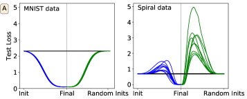
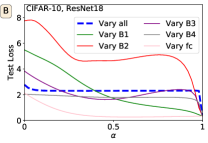
Figure 1: (A) Left: MNIST data. Right: spiral data. Test loss over 10 runs for a two hidden layer MLP along the linear path between: $\theta_{i}$ and $\theta_{f}$ (blue), $\theta_{f}$ and $\theta^{\prime}_{i}$ (green), $\theta_{i}$ and $\theta^{\prime}_{i}$ (black). (B) Test loss when interpolating for convolutional blocks (denoted as B), fully connected layer (fc), or the entire network (blue dashed line) for a ResNet-18 architecture on CIFAR-10 data, averaged over 10 runs.

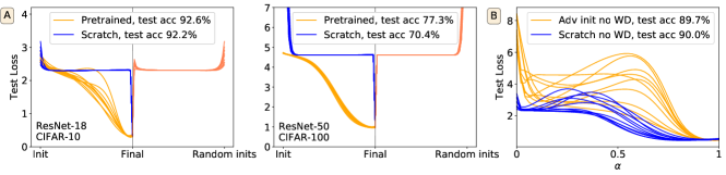
Figure 2: (A) Test loss between $\theta_{i}$ and $\theta_{f}$ of a ResNet-18 for CIFAR-10 (left) and ResNet-50 for CIFAR-100 (middle), when trained from scratch (blue) or pre-trained on ImageNet (orange) over 10 runs. Orange-red lines represent the linear path between $\theta_{f}$ (trained from pre-trained) to $\theta^{\prime}_{i}$. (B) Test loss between $\theta_{i}$ and $\theta_{f}$ of a ResNet-18 trained with SGD without weight decay (WD) on CIFAR-10 either from scratch (blue) or from a network pre-trained on 100% random labels (orange).

Defining barriers. We consider the linear path to contain a barrier if it exhibits a monotonic increase in loss. Goodfellow et al. (2015) observed that, for fully-connected networks on MNIST data, loss decays monotonically along the linear path between initial and trained model, i.e., there are no barriers. Figure 1A (left) reproduces this behaviour for an MLP with two hidden layers trained on MNIST (blue) (full details in Appendix A); moreover, the same monotonic decrease occurs when interpolating between these final weights and any random initialization (green). However, this barrier-free linear interpolation is not a universal phenomenon. As a counterexample, when using the exact same architecture and optimizer but a different dataset (the spiral dataset), barriers do appear along the linear path (Figure 1A, right), in fact rising above the level of loss at initialization; barriers rise even higher when interpolating to other initializations.

Barriers in modern neural network architectures. Frankle (2020) and Lucas et al. (2021) updated the results of Goodfellow et al. (2015) by studying linear interpolation in modern vision settings. Both observed that, in many cases, “loss plateaus and error remains at the level of random chance…until near the optimum” (Frankle, 2020); that is, loss remains flat, neither monotonically decreasing or encountering barriers. Our results for a ResNet-18 on CIFAR-10 agree with these findings when interpolating for the entire network as the dashed blue line in Figure 1B illustrates.

Block-wise interpolation. Individual convolutional blocks behave differently from the full network. As the solid lines in Figure 1B show, different blocks take on a variety of behaviors including barriers and monotonic decay. This suggests that it may be valuable to study the connection between linear interpolation and other properties of the network at the finer granularity of individual structural components rather than at the coarse granularity of the entire network.

4 The Role of Initialization

The choice of initialization affects the path that the model follows and the optimum it finds. It is therefore natural to believe that it also affects the nature of the loss when linearly interpolating from start to finish, a relationship we study in this section. We observe an intuitive relationship between initialization and barriers: actions that make the task easier (e.g., pre-training the model or initializing at the barrier) remove barriers, while those that make the task harder (e.g., initializing adversarially) increase the size of barriers. Pre-training only certain layers can both create barriers and worsen test accuracy, although not in a correlated fashion.

Pre-training. Training a model from a pre-trained state (on ImageNet) causes the loss along the linear path to monotonically decay and improves test accuracy (Figure 2A). This is distinct from the behavior when interpolating to a new random initialization, which exhibits a plateau. This result aligns with the intuition that pre-training simplifies optimization (Hao et al., 2019; Neyshabur et al., 2020).

Adversarial initialization. We perform adversarial initialization by training on 100% random labels until 100% training accuracy is reached and use this state as initialization for training. In the absence of weight decay, pre-training a ResNet-18 on random labels lowers the final test accuracy (Liu et al., 2020) and increases the barrier height between initial and final state (Figure 2B). This directly opposes the effect of pre-training (Figure 2A), suggesting adversarial initialization complicates optimization.

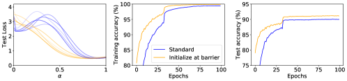
Figure 3: ResNet-18 on CIFAR-10 without weight decay. Left: test loss between $\theta_{i}$ and $\theta_{f}$, when trained either from scratch (blue) or from a initialization corresponding to the height of the barrier along each blue line (orange). Initialization at the height of the barrier removes the presence of a barrier (left), speeds up training (middle), and improves the test accuracy (right), averaged over 5 runs.

Method	Test acc (%)
T-All but RI-1	91.79 $\pm$0.23
T-All but RI-2	91.83 $\pm$0.21
T-All but RI-3	92.35 $\pm$0.20
T-All but RI-4	90.97 $\pm$0.31
P-All but RI-1	89.97 $\pm$0.13
P-All but RI-2	89.91 $\pm$0.21
P-All but RI-3	91.78 $\pm$0.22
P-All but RI-4	92.78 $\pm$0.22

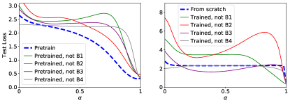
Figure 4: We set a ResNet-18 to a pre-trained (P) (middle) or trained (T) (right) state, but re-set a specific convolutional block (B) to a random initialization (RI). Then we train as usual on CIFAR-10. This often affects the test accuracy of the final model (left). Sometimes barriers appear along the linear path for the full net between $\theta_{i}$ and $\theta_{f}$ (middle/right), averaged over 10 runs.

Height of the barrier initialization. The linear path of a ResNet-18 trained without weight decay on CIFAR-10 exhibits barriers for some random seeds. For the runs that exhibit barriers, we save the model state at the height of the barrier and use this as initialization for training to study if there exists a barrier between this state and the new optimum. Although it was initialized at a higher loss than occurs at random initialization, the resulting network obtains a higher test accuracy than the network trained from scratch and its linear path is barrier free (Figure 3). This mirrors the pre-training results (Figure 2A), suggesting initialization at the height of the barrier aids optimization.

Partial pre-training. Zhang et al. (2019) measured the change in test accuracy when re-setting specific layers of a trained neural network to their initial state and found large differences across layers. To extend this work, one can study the loss from the initial state of a specific layer to its final state, while keeping all other layers fixed at their final state (Chatterji et al., 2020). We found that the shape of this path greatly varies per convolutional block of a ResNet-18 (Figure 1B). But what these studies do not address is the effect of different layer-wise (or block-wise) initialization on training itself. We thus introduce the concept of “partial (pre-)training”: we first train on CIFAR-10 (or pre-train on ImageNet) and then re-set a specific convolutional block to its initial (random) state, while keeping the other parameters at their (pre-)trained state. We then use this state of the model as initialization and train as usual on CIFAR-10 data.

We find that while pre-training a ResNet-18 leads to higher test accuracy (Figure 2A), partial pre-training often leads to a lower accuracy of the final trained network (Figure 4, left) compared to training the net from scratch. Further, while pre-training the full net leads to monotonic decay along the linear path between initial and final state (Figure 2A), partial pre-training often generates barriers (Figure 4). The sensitivity of the network to partial pre-training varies per convolutional block and also between the trained and pre-trained setting (e.g., when re-setting convolutional block 4 (RI-4), using a trained state for the rest of the net (T-All) strongly affects test accuracy, but using a pre-trained state (P-All) does not). We conclude that the choice of initialization for different convolutional blocks strongly affects test accuracy after training and changes the nature of optimization. It is remarkable that using a random initialization for the full net leads to higher test accuracy than using a partially pre-trained or partially trained net as initialization.

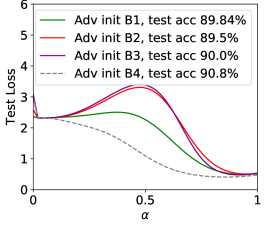
Figure 5: ResNet-18 on CIFAR-10 without weight decay. Test loss between $\theta_{i}$ and $\theta_{f}$ when one conv block (B) was adversarially initialized using random labels, averaged over 10 runs.

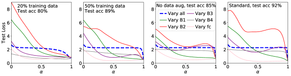
Figure 6: Test loss between $\theta_{i}$ and $\theta_{f}$ for ResNet-18 on CIFAR-10 when varying the amount of training data and whether data augmentation (horizontal flips, random crops) is used. Averaged over 10 runs.

Block-wise adversarial initialization. To further explore the effect of using different initializations for individual convolutional blocks on the linear path and test accuracy, we set one convolutional block to a random label adversarial initialization while using a standard random initialization for the rest of the net. We then re-train using this initialization. We find that while adversarial initialization for the first convolutional blocks lowers the test accuracy, using adversarial initialization for convolutional block 4 slightly increases the final test accuracy compared to training from scratch (Figure 5). This is also reflected by the shape of the linear path: when using an adversarial initialization for convolutional block 4 the linear path exhibits monotonic decay while others settings exhibit barriers.

Summary. Whereas the use of pre-training removes the presence of barriers and increases test accuracy, the use of adversarial initialization increases barriers and lowers test accuracy. Initializing neural networks at the height of the barrier along their initial to converged state leads to monotonic decay along the linear path, speeds up training, and improves test accuracy. Further, we find that certain convolutional blocks are more sensitive to partial pre-training than others, but the change in test accuracy is not correlated with the shape of the linear path. Whereas pre-training of the full net increases test accuracy and leads to monotonic decay, partial pre-training typically worsens the test accuracy of the resulting net and can generate barriers.

5 The Role of the Dataset

As illustrated in Figure 1A, where we used the same architecture, initialization, and optimizer to train on two different datasets, the data has a direct influence on the behaviour when linearly interpolating. In this section, we further investigate the effect of data on interpolation.

Number of examples. When only a subset of the training data set is used throughout training, we expect optimization to be easier and faster, yet the test accuracy of the final model is typically lowered. We find that using a smaller amount of CIFAR-10 training data induces monotonic decay when interpolating and lowers test accuracy (Figure 6, left).

Role of data augmentation. Throughout this work we use a horizontal flip and random crop as data augmentation for CIFAR-10. Removing data augmentation lowers the layer-wise barriers along the linear path (Figure 6, center right). In Appendix D, we show that increasing data augmentation increases the height of layer-wise barriers, while removing data augmentation when using only a subset of the training data further reduces the presence of layer-wise barriers.

Summary. The shape of the layer-wise linear path is affected by changes to the data, but the shape of the full model linear path is less representative (blue dashed lines, Figure 6). Reducing the complexity of the task (e.g., reducing the amount of data or removing augmentation) lowers or removes layer-wise barriers. The setting with the highest layer-wise barriers reaches the highest test accuracy, and the setting without barriers reaches the lowest test accuracy.

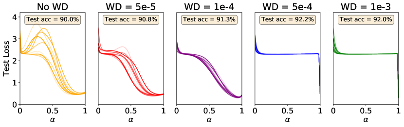
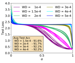
Figure 7: Effect of the amount of weight decay (WD) used for training ResNet-18 on CIFAR-10 on the linear path and test accuracy. The highest test accuracy is reached using WD =5e-4 (blue).

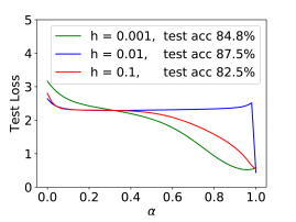
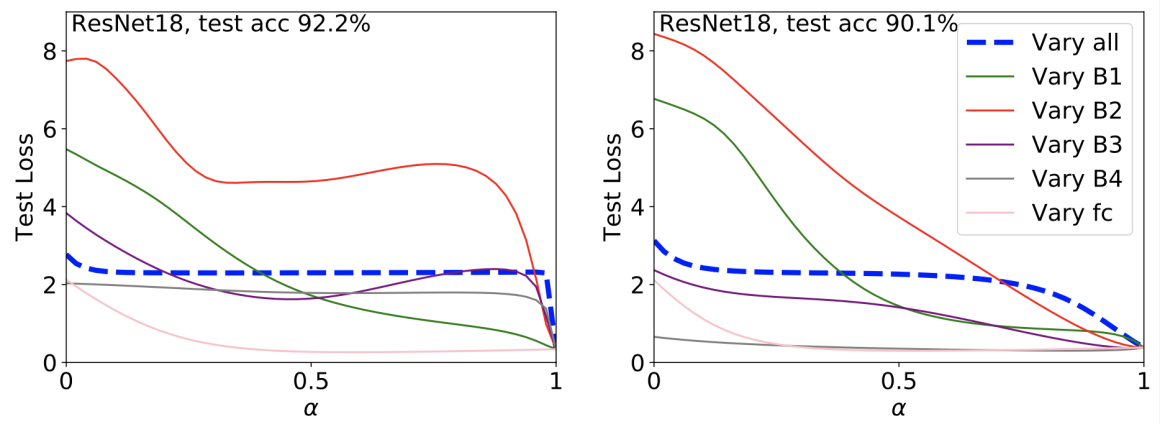
Figure 8: ResNet-18 trained on CIFAR-10 with fixed learning rate $h$. Averaged over 10 runs.

Figure 9: Block-wise linear interpolation for ResNet-18 trained on CIFAR-10 using different initial learning rates $h_{0}$. Left: $h_{0}=0.1$ for all, right: $h_{0}$ = 0.01 for layers/conv. blocks that exhibit barriers and $h_{0}$ = 0.1 for the rest.

6 The Role of the Optimizer

Optimizer hyperparameter settings, such as the learning rate and weight decay values, strongly affect which optimum is found and the test accuracy. Further, Lucas et al. (2021) found that training modern vision networks with Adam (as opposed to the more typical SGD with momentum) more frequently leads to non-monotonic decay of the loss when linearly interpolating. Adam also increases the distance that the network travels from initialization, leading Lucas et al. (2021) to posit “large distances moved in weight space encourage non-monotonic interpolation”. Inspired by this, we study how using different levels of weight decay or different fixed learning rates —both of which affect the distance travelled and final accuracy— affect the shape of loss when linearly interpolating. We find that the hypothesis of Lucas et al. (2021) does not hold in general and that the level of weight decay directly controls the behaviour along the linear path.

The effect of weight decay on linear interpolation. In Figure 9, we vary the amount of weight decay (WD) that is used to train ResNet-18 on CIFAR-10 data. When using little or no weight decay, the behaviour of the loss varies over different runs; it sometimes exhibits barriers and sometimes monotonic decay. When using more weight decay, the behaviour changes. At 1e-4 (purple), the loss consistently monotonically decays. The highest test accuracy is reached when training with 5e-4 (blue), for which loss consists of a plateau with a sudden drop close to the final state. When increasing beyond that, test accuracy decreases, but the loss still exhibits a plateau. The shape of the linear path is thus not a reliable indicator of test accuracy of the final model.

How do barriers connect to the distance travelled? Non-monotonic behaviour occurs when training a model both with zero and large weight decay values (Figure 9), while we would expect models without weight decay to travel farther. To further study this relationship, we trained a ResNet-18 at different fixed learning rates $h$ (Figure 9). The linear paths for models trained using higher and lower learning rates ($h=0.1$ and $0.001$) exhibit monotonic decay, while training with an intermediate learning rate ($h=0.01$) does not. This contradicts the hypothesis of Lucas et al. (2021), under which we would expect the model with the highest learning rate (which travels the furthest) to have a barrier, not a model with a lower learning rate. In addition, these results also cast doubt on a connection between monotonically decreasing loss and better accuracy; the middle learning rate (the one that induces a barrier) reaches higher test accuracy than either of the other learning rates (which do not).

Layer-wise sensitivity to learning rate. We have observed that linear interpolation behaviour varies by layer (Figure 1B) and that layers/individual conv blocks have different levels of sensitivity to the choice of initialization (Figure 4 and Figure 5). This raises the question of how the use of different optimizer hyperparameter choices for different layers affects the shape of the linear path and the final test accuracy of the model. Figure 9 shows the effect of training layers that exhibit barriers with a different learning rate than those that do not. Lowering the initial learning rate used for layers that exhibit barriers removes those barriers, but also substantially lowers the test accuracy of the final model.

Summary. The distance between initial and final state is not a reliable indicator of non-monotonic behaviour. The shape of the linear path is directly influenced by the amount of weight decay and is not indicative of test accuracy. Training layers that exhibit barriers with a smaller initial learning rate removes the barriers, but also lowers test accuracy.

7 The Role of the Model

Throughout this work we focused on a ResNet-18 architecture with batch normalization. We now discuss the role of the model architecture on the shape of the linear path.

Architecture depth. Generally, the use of deeper ResNet architectures on CIFAR-10 data generates or increases the height of convolutional block-wise barriers (Figure 10).

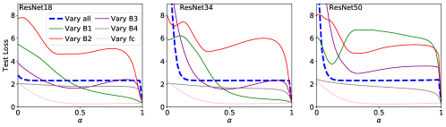
Figure 10: Test loss when interpolating for convolutional blocks (denoted as B) and the entire network (blue dashed line) for different ResNet architectures trained from scratch on CIFAR-10 data. Results are averaged over 10 runs.

Role of batch normalization. Similar to Lucas et al. (2021), we find that the use of batch normalization (BN) leads to non-monotonic behaviour along the linear path for ResNet and VGG architectures (see Appendix F). However, we find that for various datasets, MLPs do exhibit barriers in the absence of BN (see e.g., Figure 1A). We also study the linear interpolation parameter group-wise and show that the running mean and variance BN parameters play an important role in the shape of the linear interpolation path observed for the full convolutional block (see Appendix F).

Summary of other architectures. In Appendix F, we show that the behaviour for VGG-11 is similar to that of a ResNet-18. For MLPs, we find that increasing the number of nodes in layers with barriers removes the overall presence of barriers. This effect does not transfer to ResNet architectures. For MLPs, early layers contain barriers, whereas later layers do not exhibit barriers. Similarly, Zhang et al. (2019) found that the first layer is most sensitive to re-initialization.

Summary. Batch normalization encourages non-monotonic behaviour. Meanwhile, in Figure 9 (and Table A3) we showed that using a large initial learning rate for layers/conv blocks that contain barriers is necessary to achieve good test accuracy. These effects together corroborate the observation by Jastrzȩbski et al. (2020) that using a large learning rate is necessary for networks with batch normalization. We also find that the behaviour for MLPs is distinct from ResNet or VGG architectures.

8 Discussion and Future Work

Throughout this work, we explored the relationship between the shape of the linear path between the initial and final model states and the outcome of optimization. We also studied the linear path in a layer-wise fashion to illustrate that individual convolutional blocks have different sensitivities to initialization and optimizer hyperparameter settings.

What influences the shape of loss when linearly interpolating? This one-dimensional slice of the landscape is heavily influenced by both initialization and optimization choices. We found that the data also directly influences the linear path (Figure 1A and Section 5). In addition, the natural language processing literature suggests that attention-based models need adaptive optimizers (e.g. Adam) to train properly (Devlin et al., 2018; Liu et al., 2019; Zhang et al., 2020), unlike convolutional models for vision data, which can be trained well with SGD with momentum (Szegedy et al., 2014; He et al., 2016; Zagoruyko & Komodakis, 2016). While we focused on the latter, we think that revisiting this study for attention-based models is an interesting direction for future work.

Does the shape of loss when interpolating provide insight into other aspects of optimization? Linear interpolation is a one-dimensional view of the high-dimensional optimization landscape. The network follows a different, nonlinear path from initialization to its final weights. As such, linear interpolation inherently sacrifices information about the optimization problem; prior work and this paper consider whether the information it gleans still provides useful insights into optimization.

Despite the intuition provided by Goodfellow et al. (2015) that the absence or presence of obstacles reflects difficulty of optimization, we found many cases where higher layer-wise barriers or the creation of barriers along the linear path of the full model appear alongside increased test accuracy. This evidence implies that either a more difficult optimization trajectory can lead to improved generalization, or Goodfellow et al.’s intuition about the relationship between interpolation and optimization difficulty does not apply to the networks we studied. Moreover, we found cases where monotonically decreasing loss was accompanied by higher test accuracy (e.g., pre-training). We also found others where the linear path exhibited both barriers and monotonic decay over different runs (e.g., weight decay) and where the presence or absence of barriers was not correlated with increased or decreased test accuracy. In short, for the settings we considered, the shape of the linear path between initial and final state was not a reliable indicator of test accuracy of the trained model. Our results show that caution is needed when using linear interpolation to make broader claims on the shape of the landscape and success of optimization.

Layer-wise interpolation. Interpolating layer-wise makes it possible to study changes in behaviour that are difficult or impossible to discern when interpolating using the full network, for example changes in the data (Figure 6) or model (Figure 10). Further, independent of the shape of the linear path, we found that partial pre-training of convolutional blocks can counterintuitively lower test accuracy of the final model; this result implicates the increasingly popular direction of training individual layers in different ways (You et al., 2017; Leimkuhler et al., 2019; Murfet et al., 2020; You et al., 2020) and raises questions about the basis upon which we should make such decisions.

9 Conclusion

We conclude that the shape of the linear path from initial to final state is not a reliable indicator of test accuracy. Although focusing on one line of analysis, e.g. on the role of initialization, seems to suggest that there does exist a connection, the full picture (Table 1, Fig. A11) illustrates that this is misleading. We believe publishing this negative result is important due to the widespread use of the linear interpolation method. Further, we introduce a new line of inquiry by studying the role played by individual layers and substructures of the network. We find that certain layers require larger initial learning rates to maintain the same test accuracy. We also show the surprising adversarial effect of partial pre-training. Further exploration of the layer-wise sensitivity to choice of initialization offers an exciting direction for future work.

Appendix A Implementation Details

Throughout the paper we focus on a ResNet-18 architecture with batch normalization trained on CIFAR-10 data. We set batchsize to 128, use cross entropy loss, and use as data augmentation: horizontal flip, random crop, and normalization. We train the network for 100 epochs using SGD with momentum with weight decay set to 5e-4 and the momentum hyperparameter set to 0.9. We use an initial learning rate of $h=0.1$ that is dropped by a factor of 10 every 33 epochs. For pre-trained models we use initial learning rate $h=0.001$ that is dropped by a factor of 10 after 30 epochs. We obtain our pre-trained models from the PyTorch library, which have been trained on ImageNet. We replace the final fully connected layer to match the number of classes and (when training on CIFAR-10 data) set the first convolutional layer to have 3 input channels, 64 output channels, and a kernel size of $3\times 3$. We perform all our experiments in PyTorch using NVIDIA DGX-1 GPUs and use standard random PyTorch initialization. Our results are all averaged across multiple runs with different random seeds on initialization and data order.

In this work we vary specific aspects of the training problem, such as the optimizer hyperparameters, data, initialization, and model, while keeping all other aspects fixed. For example, we consider deeper ResNet architectures (Figure 10), but use the same optimizer, data, and initialization settings as for our base model. But, as described in the paper, there are a few experiments where we change multiple aspects of the training problem: we turn off weight decay for both our random label initialization experiment (Figure 2B) and our height of barrier initialization experiment (Figure 3). For the former, we wanted to study the effect of adversarial initialization that lowered the test accuracy of the final trained network. A network trained on 100% random labels as initialization typically does not affect the test accuracy of the final model, when using SGD with momentum, learning rate decay and weight decay (Liu et al., 2020). But turning off weight decay during training in combination with pre-training on random labels does lower the test accuracy. For our height of barrier initialization experiment (Figure 3) we needed a setting for which the linear path exhibited clear barriers. For a ResNet-18 this is found for some seeds when weight decay is turned off (Figure 9). For the runs that exhibited barriers we saved the state of the model at the height of this barrier and used this as initialization for our model to produce Figure 3.

Further, to obtain Figure 1A we used a two hidden layer perceptron with 50 nodes in each hidden layer and ReLU activations. We used Adam with $h=$ 5e-4, without weight decay or any learning rate scheduling. We use batch size 128 for MNIST data and cross entropy loss. We use binary cross entropy loss for the binary classification spiral data set. The first class of the spiral data set is generated using

$$x =2\sqrt{t}\cos(8\sqrt{t}\pi)+0.02\mathcal{N}(0,1),$$

$$y =2\sqrt{t}\sin(8\sqrt{t}\pi)+0.02\mathcal{N}(0,1),$$ (3)

where $t$ is drawn repeatedly from the uniform distribution $\mathcal{U}(0,1)$ to generate data points. The other class of this dataset is obtained by shifting the argument of the trigonometric functions by $\pi$. For our experiments on the spiral data set we used 10000 training data, 5000 test data points and a batch size of 500.

Appendix B Overview of Results

A summary of all our findings can be found in Figure A11.

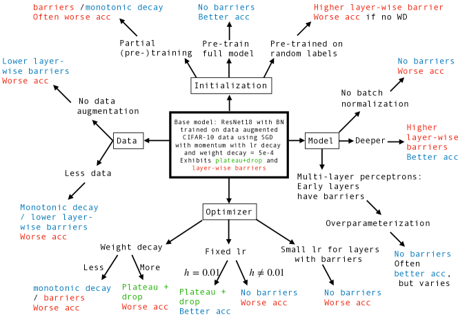
Figure A11: The linear path between $\theta_{i}$ and $\theta_{f}$ of our base ResNet-18 architecture exhibits a plateau at the level of random chance until close to the optimum (plateau + drop); it exhibits barriers when evaluating the linear path layer-wise (see Figure 1B). The base model obtains 92.2% accuracy on CIFAR-10 test data. In this figure we present the change in test accuracy and shape of the linear path between $\theta_{i}$ and $\theta_{f}$ compared to this base model along four axes: the optimizer, the data, the initialization, and the model. The presence of barriers (indicated in red) frequently coincides with a better test accuracy (indicated in blue).

Appendix C Further Studies on the Role of Initialization

Left/right of barrier initialization. In Section 4 we showed the effect of initializing neural networks at the parameter configuration which corresponds to the height of the barrier along their initial to converged state. We considered a ResNet-18 architecture which was trained without weight decay on CIFAR-10 data. The linear interpolation path in this setting clearly exhibits barriers for some seeds (Section 6, Figure 9). For the runs that exhibited barriers, we saved the model state at the the height of the barrier and used this as initialization for our model. Although it was initialized at a higher loss than occurs at random initialization, the resulting network obtained a higher test accuracy than the network trained from scratch and its linear path exhibited monotonic decay (Figure 3). In Figure A12 and Table A2 we show that these effects are not restricted to initialization at the barrier: choosing an initialization along the linear path to the left or the right of the barrier leads to similar performance improvement (Table A2) and typically monotonic decay along the linear path (Figure A12).

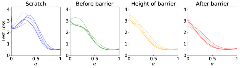
Figure A12: ResNet-18 on CIFAR-10 without weight decay. Test loss between $\theta_{i}$ and $\theta_{f}$ for discrete set of $\alpha\in[0,1]$ in 50 equally spaced subintervals, when trained either from scratch (blue) or from an initialization corresponding to $\theta_{\alpha}$ of the blue line at: the height of the barrier $\alpha_{\text{barrier}}$ (orange), just before the barrier at $\alpha=\alpha_{\text{barrier}}-5$ (green), just after the barrier at $\alpha=\alpha_{\text{barrier}}+5$ (red).

Table A2: ResNet-18 on CIFAR-10 without weight decay. Test loss between $\theta_{i}$ and $\theta_{f}$ for discrete set of $\alpha\in[0,1]$ in 50 equally spaced subintervals, when trained either from scratch (blue) or from an initialization corresponding to $\theta_{\alpha}$ of the blue line at: the height of the barrier $\alpha_{\text{barrier}}$, before the barrier at $\alpha=\alpha_{\text{barrier}}-5$, after the barrier at $\alpha=\alpha_{\text{barrier}}+5$ (red).

Initialization	Training accuracy (%)	Test accuracy (%)
Random initialization	99.44 $\pm$0.12	90.01 $\pm$0.39
Before barrier	99.80 $\pm$0.04	91.05 $\pm$0.21
Height of barrier	99.86 $\pm$0.02	91.12 $\pm$0.18
After barrier	99.88 $\pm$ 0.02	90.85 $\pm$0.17

Block-wise adversarial initialization with different levels of weight decay. To further explore the effect of using different initializations for individual convolutional blocks on the linear path and test accuracy, we set one convolutional block to a random label adversarial initialization while using a standard random initialization for the rest of the net. We then re-train using this initialization with different amounts of weight decay (WD). We vary the WD value to study how changes in the full model linear path (Figure 9) are reflected by the convolutional block-wise linear path. We find that while adversarial initialization for the first convolutional blocks lowers the test accuracy, using adversarial initialization for convolutional block 4 slightly increases the final test accuracy compared to training from scratch (compare Figure A13 with Figure 9). This is also reflected by the shape of the linear path: when using an adversarial initialization for convolutional block 4 the linear path exhibits monotonic decay while others settings exhibit barriers (no WD) and a barrier while other settings exhibit a plateau (WD = 5e-4).

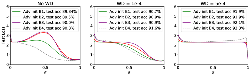
Figure A13: Test loss between $\theta_{i}$ and $\theta_{f}$ when one specific conv block (B) was adversarially initialized using random labels. The net was trained either without weight decay (WD) (left), with WD = 1e-4 (middle) or with WD = 5e-4 (right). Averaged over 10 runs.

Appendix D Further Studies on the Role of Data

Less training data and no data augmentation. Further to our experiments in Section 5, we here show the combined effect of reducing the number of training data in addition to removing data augmentation (Figure A14, left). We find that although this further reduces the test accuracy and presence of block-wise barriers, the overall behaviour for the linear interpolation of the full model (blue dotted line) is maintained (unless the number of training data is further reduced, see Figure 6, left in main paper).

Figure A14: Test loss between $\theta_{i}$ and $\theta_{f}$ for ResNet-18 on CIFAR-10 when varying the amount of training data and whether data augmentation (horizontal flips and random crops) is used.

More data augmentation. In Figure A15 we show that using additional data augmentation causes the height of layer-wise barriers to slightly increase (for B2 and B3).

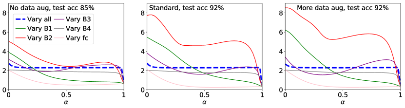
Figure A15: Test loss between $\theta_{i}$ and $\theta_{f}$ for ResNet-18 on CIFAR-10 when using either no data augmentation (left), standard data augmentation (horizontal flips and random crops) (middle), or additional data augmentation (brightness = 0.05) (right).

Appendix E Further Studies on the Role of Optimization

Distance. In our fixed learning rate experiment (Figure 9) we showed that setting $h=0.01$ leads to the largest test accuracy of the trained model and non-monotonic behaviour of the loss along the linear path between initial and final state. Meanwhile using a larger ($h=0.1$) or smaller ($h=0.001$) learning rate led to a lower test accuracy and monotonic decay of the loss along the linear path. We used the same initialization to compare the different settings, but averaged the results presented in Figure 9 over 10 runs using different random seeds. To measure the distance between initial $\theta_{i}$ and final $\theta_{f}$ models we use the following measure (as used in (Liu et al., 2020)):

$$d(\theta_{f},\theta_{i})=\frac{\|\theta_{f}-\theta_{i}\|_{F}}{\|\theta_{i}\|_{F}},$$ (4)

where $\|\cdot\|_{F}$ denotes the Frobenius norm. There exist many other ways of measuring the distance, which affect the order of magnitude. Since we focus only on the relative distances travelled for different learning rate settings the use of Eq. (4) suffices for this purpose. We find that the average distance travelled when using $h=0.1$ is 1.03, whereas the average distance travelled when using $h=0.01$ is 0.88 and when using $h=0.001$ is 0.22. This confirms our intuition that using a larger learning rate will increase the distance travelled.

Custom optimization schemes. We observed that using a smaller initial learning rate for layers or convolutional blocks which exhibit barriers removes these barriers, but also lowers the test accuracy of the resulting model for a ResNet-18 architecture (Figure 9 or Figure A16A). We observe the same behaviour for a VGG-11 architecture (Figure A16B). We consider layers (or convolutional blocks) to not exhibit barriers if the loss along their linear path is monotonically decreasing; the exact layers are specified in the caption of Figure A16.

The changes in linear interpolation behaviour per layer, raises the question whether we can optimize different layers differently depending on the absence or presence of barriers. Table A3 shows the result of using custom optimization schemes that train layers (or convolutional blocks) that exhibit barriers with a different learning rate or amount of weight decay than those that do not. Lowering the initial learning rate used for layers without barriers or eliminating weight decay has a smaller (ResNet-18) or no (VGG-11) effect on the test accuracy of the trained model, whereas doing so for layers with barriers or for the full model does significantly affect performance.

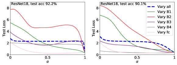
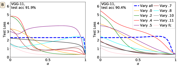
Figure A16: Layer-wise (or block-wise) linear interpolation for ResNet-18 (A) and VGG-11 (B) trained from scratch on CIFAR-10 data using different initial learning rates $h_{0}$. For ResNet-18 (A): left: $h_{0}=0.1$ for all, right: $h_{0}$ = 0.01 for conv block 2, 3, and 4.0 and $h_{0}$ = 0.1 for rest. For VGG-11 (B): left: $h_{0}=0.1$ for all, right: $h_{0}$ = 0.01 for layers 4-10 and $h_{0}$ = 0.1 for rest. Using smaller learning rates for layers that exhibit barriers (ResNet-18: conv block 2, 3, and 4.0, VGG-11: layer 4-10) can remove barriers, but lowers the test accuracy of the resulting model.

Table A3: We train layers that exhibit barriers (B) with a different learning rate or amount of weight decay (WD) than those that do not (NB). Test accuracy is maintained much better when training only the layers with barriers at the higher learning rate or with weight decay. Results are averaged over 10 runs.

	Test accuracy
Initial learning rate $h_{0}$	ResNet-18	VGG-11
$0.1$ (all)	92.2 $\pm$0.2%	91.9 $\pm$0.2%
$0.1$ (B), $0.01$ (NB)	91.8 $\pm$0.2%	92.0 $\pm$0.1%
$0.01$ (B), $0.1$ (NB)	90.1 $\pm$0.2%	90.4 $\pm$0.1%
$0.01$ (all)	90.3 $\pm$0.3%	90.9 $\pm$0.1%
WD (B), No WD (NB)	91.5 $\pm$0.2%	91.8 $\pm$0.1%
No WD (B), WD (NB)	90.1 $\pm$0.3%	90.2 $\pm$0.1%
No WD (all)	90.1 $\pm$0.4%	90.4 $\pm$0.3%

Appendix F Further Studies on the Role of the Model

Multi-layer perceptrons. For multi-layer perceptrons (MLPs) we find that the early layers (close to the input) typically exhibit barriers, whereas later layers exhibit monotonic decay (Figure A17, left). By increasing the number of nodes in layers that exhibit barriers one can reduce the presence of barriers for the overall model (Figure A17, middle). Meanwhile, layers that do not exhibit barriers can be narrowed without removing the monotonic decay property (Figure A17, right).

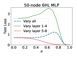
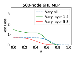
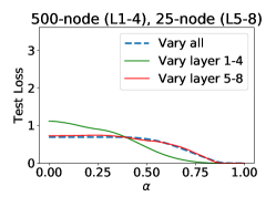
Figure A17: A 6 hidden layer MLP trained on spiral data (generated using Eq. 3) using different amount of nodes in the hidden layers: 50-node for all layers (left), 500-node for all layers (middle), 500-node for layers that exhibit barriers (layer 1-4) and 25-node for layers that exhibit monotonic decay (layer 5-8) (right). All approaches obtain 100% test accuracy. Increasing the number of nodes in layers that exhibit barriers removes the presence of barriers for the overall model (blue dotted line).

Batch normalization. In Figure A18 we show using parametergroup-wise linear interpolation that the running mean and variance batch normalization parameters appear to govern the behaviour of the full convolutional block. For the linear path of the full model, we corroborate the findings of (Lucas et al., 2021) that the use of batch normalization often leads to non-monotonic behaviour (Figure A19). In the absence of batch normalization, ResNet and VGG architectures often exhibit monotonic decay along their linear path from initial to final state. However, for various datasets we find that MLPs do exhibit barriers in the absence of batch normalization, see e.g., Figure A17.

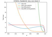
Figure A18: We keep all parameters of a ResNet-18 architecture fixed at their final trained position (on CIFAR-10 data), apart from specific parameter groups in the third convolutional block, which we vary from their initial to final position using the linear interpolation technique. The blue line is when the full third convolutional block is varied. The batch normalization parameters are split into two groups, the running mean and variance (red) and the others (green).

VGG-11. In Figure A19 we show the loss along the linear path for a VGG-11 architecture on CIFAR-10 data with (left) and without (right) batch normalization.

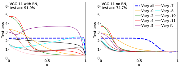
Figure A19: Test loss between $\theta_{i}$ and $\theta_{f}$ for VGG-11 on CIFAR-10 when varying whether batch normalization (BN) is used.

Layer width: We find for a VGG-11 architecture with batch normalization on CIFAR-10 data that layers without barriers can be narrowed without affecting the generalization performance (Table A4). This does not hold for layers that do exhibit barriers along the linear path between the initial and final state. We found that this effect did not generalize to a ResNet-18 architecture, so recommend caution with using the presence or absence of layer-wise layers as an indication of which layers can be narrowed.

Table A4: Layer-wise linear interpolation for a VGG-11 architecture with batch normalization trained from scratch on CIFAR-10 data. This architecture exhibits no barriers in the first two layers, final layer and the fully connected layer, whereas it does exhibit barriers in the five middle layers (see also Figure A19, left). We find that narrowing all non-barrier layers by half only marginally lowers the test accuracy (2nd row), whereas narrowing only one barrier layer (3rd row) already has a large impact. Narrowing two (4th row) or all barrier layers (final row) lowers the test accuracy even further.

Intervention	Test accuracy (%)
Standard	91.93 $\pm$0.19
Narrow no-barrier layers	91.73 $\pm$0.19
Narrow   1 barrier layer	91.53 $\pm$0.20
Narrow   2 barrier layers	91.25 $\pm$0.12
Narrow all barrier layers	91.15 $\pm$0.13

References

- Chatterji et al. (2020) Chatterji, N. S., Neyshabur, B., and Sedghi, H. The intriguing role of module criticality in the generalization of deep networks. ICLR, 2020.
- Devlin et al. (2018) Devlin, J., Chang, M.-W., Lee, K., and Toutanova, K. BERT: Pre-training of deep bidirectional transformers for language understanding. arXiv preprint arXiv:1810.04805, 2018.
- Draxler et al. (2018) Draxler, F., Veschgini, K., Salmhofer, M., and Hamprecht, F. A. Essentially no barriers in neural network energy landscape. arXiv:1803.00885, 2018.
- Fort & Jastrzebski (2019) Fort, S. and Jastrzebski, S. Large scale structure of neural network loss landscapes. ICML, 2019.
- Fort et al. (2019) Fort, S., Hu, H., and Lakshminarayanan, B. Deep ensembles: A loss landscape perspective. Bayesian Deep Learning workshop, NeurIPS, 2019.
- Frankle (2020) Frankle, J. Revisiting “qualitatively characterizing neural network optimization problems”. ML Retrospectives NeurIPS workshop, 2020.
- Garipov et al. (2018) Garipov, T., Izmailov, P., Podoprikhin, D., Vetrov, D. P., and Wilson, A. G. Loss surfaces, mode connectivity, and fast ensembling of DNNs. NIPS, 31:8789–8798, 2018.
- Goodfellow et al. (2013) Goodfellow, I., Warde-Farley, D., Mirza, M., Courville, A., and Bengio, Y. Maxout networks. ICML, 2013.
- Goodfellow et al. (2015) Goodfellow, I., Vinyals, O., and Saxe, A. Qualitatively characterizing neural network optimization problems. ICLR, 2015.
- Hao et al. (2019) Hao, Y., Dong, L., Wei, F., and Xu, K. Visualizing and understanding the effectiveness of BERT. EMNLP, 2019.
- He et al. (2016) He, K., Zhang, X., Ren, S., and Sun, J. Deep residual learning for image recognition. In Proceedings of the IEEE conference on computer vision and pattern recognition, pp. 770–778, 2016.
- Huang et al. (2017) Huang, G., Li, Y., Pleiss, G., Liu, Z., Hopcroft, J., and Weinberger, K. Snapshot ensembles: Train 1, get M for free. ICLR, 2017.
- Im et al. (2016) Im, D., M.Tao, and Branson, K. An empirical analysis of deep network loss surfaces. arXiv:1612.04010, 2016.
- Izmailov et al. (2018) Izmailov, P., Podoprikhin, D., Garipov, T., Vetrov, D., and Wilson, A. G. Averaging weights leads to wider optima and better generalization. Uncertainty in Artificial Intelligence, 2018.
- Jastrzȩbski et al. (2018) Jastrzȩbski, S., Kenton, Z., Arpit, D., Ballas, N., Fischer, A., Bengio, Y., and Storkey, A. Three factors influencing minima in SGD. ICANN, 2018.
- Jastrzȩbski et al. (2020) Jastrzȩbski, S., Szymczak, M., Fort, S., Arpit, D., Tabor, J., Cho, K., and Geras, K. The break-even point on optimization trajectories of deep neural networks. ICLR, 2020.
- Keskar et al. (2017) Keskar, N., Mudigere, D., Nocedal, J., Smelyanskiy, M., and Tang, P. On large-batch training for deep learning: generalization gap and sharp minima. ICLR, 2017.
- Krizhevsky & Hinton (2009) Krizhevsky, A. and Hinton, G. Learning multiple layers of features from tiny images. 2009.
- Leimkuhler et al. (2019) Leimkuhler, B., Matthews, C., and Vlaar, T. Partitioned integrators for thermodynamic parameterization of neural networks. Foundations of Data Science, 1(4):457–489, 2019.
- Li et al. (2018a) Li, C., Farkhoor, H., Liu, R., and Yosinski, J. Measuring the intrinsic dimension of objective landscapes. ICLR, 2018a.
- Li et al. (2018b) Li, H., Xu, Z., Taylor, G., Studer, C., and Goldstein, T. Visualizing the loss landscape of neural nets. NIPS, 2018b.
- Liu et al. (2020) Liu, S., Papailiopoulos, D., and Achlioptas, D. Bad global minima exist and SGD can reach them. NeurIPS, 2020.
- Liu et al. (2019) Liu, Y., Ott, M., Goyal, N., Du, J., Joshi, M., Chen, D., Levy, O., Lewis, M., Zettlemoyer, L., and Stoyanov, V. RoBERTa: A robustly optimized BERT pretraining approach. arXiv:1907.11692, 2019.
- Lucas et al. (2020) Lucas, J., Bae, J., Zhang, M., Ba, J., Zemel, R., and Grosse, R. On monotonic linear interpolation of neural network parameters. OptML NeurIPS workshop, 2020.
- Lucas et al. (2021) Lucas, J., Bae, J., Zhang, M., Fort, S., Zemel, R., and Grosse, R. Analyzing monotonic linear interpolation in neural network loss landscapes. ICML, 2021.
- McCandlish et al. (2018) McCandlish, S., Kaplan, J., Amodei, D., and Team, O. D. An empirical model of large-batch training. arXiv:1812.06162, 2018.
- Murfet et al. (2020) Murfet, D., Wei, S., Gong, M., Li, H., Gell-Redman, J., and Quella, T. Deep learning is singular, and that’s good. arXiv:2010.11560, 2020.
- Neyshabur et al. (2020) Neyshabur, B., Sedghi, H., and Zhang, C. What is being transferred in transfer learning? NeurIPS, 2020.
- Paszke et al. (2017) Paszke, A., Gross, S., Chintala, S., Chanan, G., Yang, E., DeVito, Z., Lin, Z., Desmaison, A., Antiga, L., and Lerer, A. Automatic differentiation in PyTorch. 2017.
- Szegedy et al. (2014) Szegedy, C., Liu, W., Jia, Y., Sermanet, P., Reed, S., Anguelov, D., Erhan, D., Vanhoucke, V., and Rabinovich, A. Going deeper with convolutions. CoRR, 2014.
- You et al. (2017) You, Y., Gitman, I., and Ginsburg, B. Large batch training of convolutional networks. arXiv preprint arXiv:1708.03888, 2017.
- You et al. (2020) You, Y., Li, J., Reddi, S., Hseu, J., Kumar, S., Bhojanapalli, S., Song, X., Demmel, J., Keutzer, K., and Hsieh, C. Large batch optimization for deep learning: training BERT in 76 minutes. ICLR, 2020.
- Zagoruyko & Komodakis (2016) Zagoruyko, S. and Komodakis, N. Wide residual networks. CoRR, 2016.
- Zhang et al. (2019) Zhang, C., Bengio, S., and Singer, Y. Are all layers created equal? arXiv:1902.01996, 2019.
- Zhang et al. (2020) Zhang, J., Karimireddy, S., Veit, A., Kim, S., Reddi, S., Kumar, S., and Sra, S. Why are adaptive methods good for attention models? NeurIPS, 2020.