THE BEAUTY OF THE RARE: $B_{(s)}\rightarrow\mu^{+}\mu^{-}$ AT THE LHCb

Abstract

The latest and improved measurements in $B^{0}_{(s)}\rightarrow\mu^{+}\mu^{-}$ processes have been performed by LHCb using full Run 1 and Run 2 data. The measurement of the branching fraction of $B^{0}_{s}\rightarrow\mu^{+}\mu^{-}$ is presented as the most precise single experiment measurement of such a rare process. While no significant excess is found for $B^{0}\rightarrow\mu^{+}\mu^{-}$, an stringent upper limit is set for its braching fraction. Both results are in agreement with SM predictions and with previous results.

1 Theoretical beauty

Flavour changing neutral currents (FCNC) are suppressed in the SM for several reasons. They are forbidden at tree level and can only take place through loop transitions involving multiple weak interactions. This adds to their branching fraction calculation loop and weak interaction suppression factors. Apart from this, they are also affected by the GIM mechanism, arising from the unitarity property of the CKM matrix.

The $B_{s}^{0}\rightarrow\mu^{+}\mu^{-}$ and $B^{0}\rightarrow\mu^{+}\mu^{-}$ decays, which will be further referred to as $B_{(s)}^{0}\rightarrow\mu^{+}\mu^{-}$, fall under this category. Such decays are even further affected by helicity suppression, originating from the relation between the spin of the $B_{(s)}^{0}$ and the helicity of the muons.

These processes can be described using effective field theory. Their decay amplitude can be written using an effective Hamiltonian as [1]:

$$\mathcal{M}(B_{(s)}^{0}\rightarrow\mu^{+}\mu^{-})=\langle\mu^{+}\mu^{-}|\mathcal{H}_{eff}|B_{(s)}^{0}\rangle\propto\sum_{i=10,S,P}C_{i}\mbox{ }\langle\mu^{+}\mu^{-}|\mathcal{O}_{i}|B_{(s)}^{0}\rangle$$ (1)

where $C_{i}$ are the perturbative Wilson coefficients and $\mathcal{O}_{i}$ are the non-perturbative Wilson operators, describing the short and long distance effects, respectively. The $B_{(s)}^{0}\rightarrow\mu^{+}\mu^{-}$ final state is purely leptonic whereas the initial state is purely hadronic, resulting in a lack of direct interaction between the two. Consequently, the matrix element in Eq. 1 can be factorised into the hadronic and leptonic parts, resulting in a very clean theoretical calculation:

$$\mathcal{M}(B_{(s)}^{0}\rightarrow\mu^{+}\mu^{-})=\sum_{i=10,S,P}C_{i}\mbox{ }\langle\mu^{+}\mu^{-}|\mathcal{O}_{i,ll}|0\rangle\otimes\langle 0|\mathcal{O}_{i,qq}|B_{(s)}^{0}\rangle$$ (2)

All these properties make $B_{(s)}^{0}\rightarrow\mu^{+}\mu^{-}$ decays extremely rare in the SM with very precise predicted time-integrated branching fraction [2]:

$$\mathcal{B}(B_{s}^{0}\rightarrow\mu^{+}\mu^{-}) = (3.66\pm 0.14)\times 10^{-9}$$

$$\mathcal{B}(B^{0}\rightarrow\mu^{+}\mu^{-}) = (1.03\pm 0.05)\times 10^{-10}$$

As a final remark, only the Wilson operator $\mathcal{O}_{10}$ describing axial vector interactions contributes to the $B_{(s)}^{0}\rightarrow\mu^{+}\mu^{-}$ processes in the SM. While this operator is strongly affected by helicity suppression, the scalar and pseudo-scalar contributions, $\mathcal{O}_{S}$ and $\mathcal{O}_{P}$, are not helicity suppressed. Apart from adding a whole new type of interaction to the process, NP might also arise from new axial vector interactions, such that $C_{10}=\mathcal{C}_{10}^{\mathrm{SM}}+\mathcal{C}_{10}^{\mathrm{NP}}$, which is currently the main sensitivity test related to the latest anomalies observed [3]. Hence, a small difference between the measured and the theoretical values of the branching fraction might be a strong hint of NP [4, 5].

2 Experimental beauty

An improved measurement of the $B_{(s)}^{0}\rightarrow\mu^{+}\mu^{-}$ branching fractions has been performed by LHCb using the full Run 1 and Run 2 data [6, 7]. To perform the analysis, a pair of opposite charged muons with invariant mass, $m_{\mu^{+}\mu^{-}}\in[4900,6000]\mathrm{MeV/c}^{2}$, are selected by requiring them to form a good-quality vertex displaced from the interaction point.

The signal yields are obtained from a maximum likelihood fit to the dimuon invariant mass. To increase the separation between signal and background, the fit is performed in bins of a Boosted Decision Tree (BDT) classifer, which categorizes events as more or less signal-like. This is done by assigning an score between 0 and 1 to each event such that, the closer the score to 0, the more background-like the event is. The BDT distribution of events for the full Run 1 and Run 2 datasets is shown in Fig. 1 where the dash green lines represent the limits of the signal mass region.

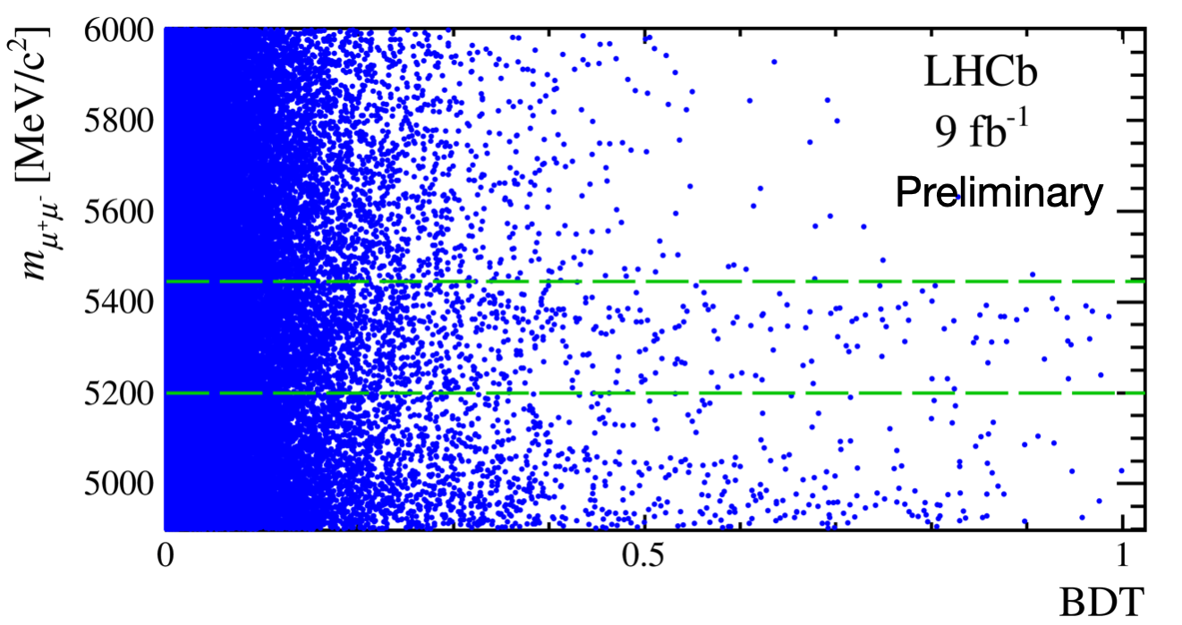
Figure 1: Distribution of events for the full dataset in BDT and invariant mass of the muons. The dashed green lines represent the signal mass region.

From the signal yields the branching fractions are determined using $B^{+}\rightarrow J/\psi K^{+}$ and $B^{0}\rightarrow K^{+}\pi^{-}$ as normalization channels, the former having similar particle identification (PID) and trigger requirements as the signal and the latter, similar kinematics.

Due to the limited statistics on the signal sample, several calibrations and estimations have to be performed to constrain the fit parameters, such as the estimation of the shapes and yields of the various backgrounds components, the signal shape calibration and the BDT calibration among others. The yields of the exclusive backgrounds are estimated from a combination of theoretical inputs, simulation and techniques based on data.

In addition, the mean and the width of the $B_{(s)}^{0}\rightarrow\mu^{+}\mu^{-}$ mass shapes, both described by a Double-Sided Crystal Ball (DSCB) function [8], are also calibrated. For the mean, fits to the invariant mass of the $B_{s}^{0}\rightarrow K^{+}K^{-}$ and $B^{0}\rightarrow K^{+}\pi^{-}$ data samples are performed using a DSCB as the mass shape. Fits to the charmonium ($J/\psi$, $\psi(2S)$) and bottonium ($\Upsilon(1S)$, $\Upsilon(2S)$, $\Upsilon(3S)$) resonances decaying to two muons are used to calibrate the width of the signal shape, which is determined from the interpolation $\sigma_{\mu\mu}(m_{\mu\mu})=a_{0}+a_{1}\cdot m_{\mu\mu}$, where the $a_{0}$ and $a_{1}$ are the interpolation constants. Finally, the tail parameters of the DSCB signal shapes are obtained from simulation samples, which are smeared with the resolution determined from the previously mentioned $\bar{q}q$ resonances.

2.1 BDT calibration

The $B_{(s)}^{0}\rightarrow\mu^{+}\mu^{-}$ decays are extremely rare processes and the measurements of their branching fractions are statistically limited. Therefore, the sensitivity of the data sample should be increased as much as possible. This is achieved by dividing the data sample in subsets of the BDT score and performing the mass fit simulatenously in all these subsets. Several binning schemes have been studied among which the best performant one has been found to be a six BDT bins scheme with the limits 0, 0.25, 0.4, 0.5, 0.6, 0.7 and 1.

As the fit is performed in bins of the BDT, the expected relative yield of $B_{(s)}^{0}\rightarrow\mu^{+}\mu^{-}$ events per BDT bin should be estimated, a procedure known as BDT calibration. The BDT calibration can be performed on corrected data, using the normalization channel $B^{0}\rightarrow K^{+}\pi^{-}$ corrected for the trigger and PID requirements, or on weighted simulation, directly from a $B^{0}_{(s)}\rightarrow\mu^{+}\mu^{-}$ simulation sample weighted to take into account the simulation and data differences. Fig. 2 displays the estimated yields of $B^{0}\rightarrow\mu^{+}\mu^{-}$ for Run 2 obtained following the two different approaches. While the former strategy was followed in the previous analysis [9], this time the latter has been analysed and used. As shown in Fig. 2, both strategies are in very good agreement and the uncertainty on the relative yields determined from the weighted simulation is significantly smaller with respect to results obtained from the previous strategy. This uncertainty reduction on the BDT calibration has a direct impact on the final uncertainty of the branching fraction measurement.

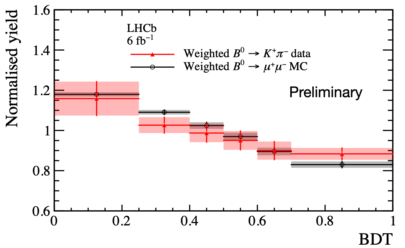
Figure 2: Expected BDT distribution for $B^{0}\rightarrow\mu^{+}\mu^{-}$ candidates using the two methods: in black $B^{0}\rightarrow\mu^{+}\mu^{-}$ weighted simulation and in red $B^{0}\rightarrow K^{+}\pi^{-}$ corrected data.

2.2 Final fit and results

The BDT calibration together with more ingredients, such as the signal calibration or the background estimation briefly mentioned before, are taken into account in the final invariant mass fit by constraining some of its parameters and shapes. Fig. 4 displays the mass distribution of the $B^{0}\rightarrow\mu^{+}\mu^{-}$ and $B^{0}_{s}\rightarrow\mu^{+}\mu^{-}$ candidates with BDT larger than 0.5 in green and red, respectively. In the same figure, the exclusive and combinatorial background distributions are also shown. From the fit, the branching fraction of $B^{0}_{s}\rightarrow\mu^{+}\mu^{-}$ is determined while a stringent upper limit is set for the $B^{0}\rightarrow\mu^{+}\mu^{-}$ branching fraction:

$$\mathcal{B}(B_{s}^{0}\to\mu^{+}\mu^{-}) = (3.09^{+0.46+0.15}_{-0.43-0.11})\times 10^{-9}$$

$$\mathcal{B}(B^{0}\to\mu^{+}\mu^{-}) < 2.6\times 10^{-10}\mbox{ at 95\% CL}$$

where the first and second uncertainties on the $B_{s}^{0}\to\mu^{+}\mu^{-}$ branching fraction correspond to the statistical and systematic uncertainties, respectively. The values measured are in good agreement with the previous results and with the SM predictions. This can also be seen from the two dimensional representation of both measured branching fractions illustrated in Fig. 4, where the contour from the previous analysis and the SM value are represented in yellow and red, respectively.

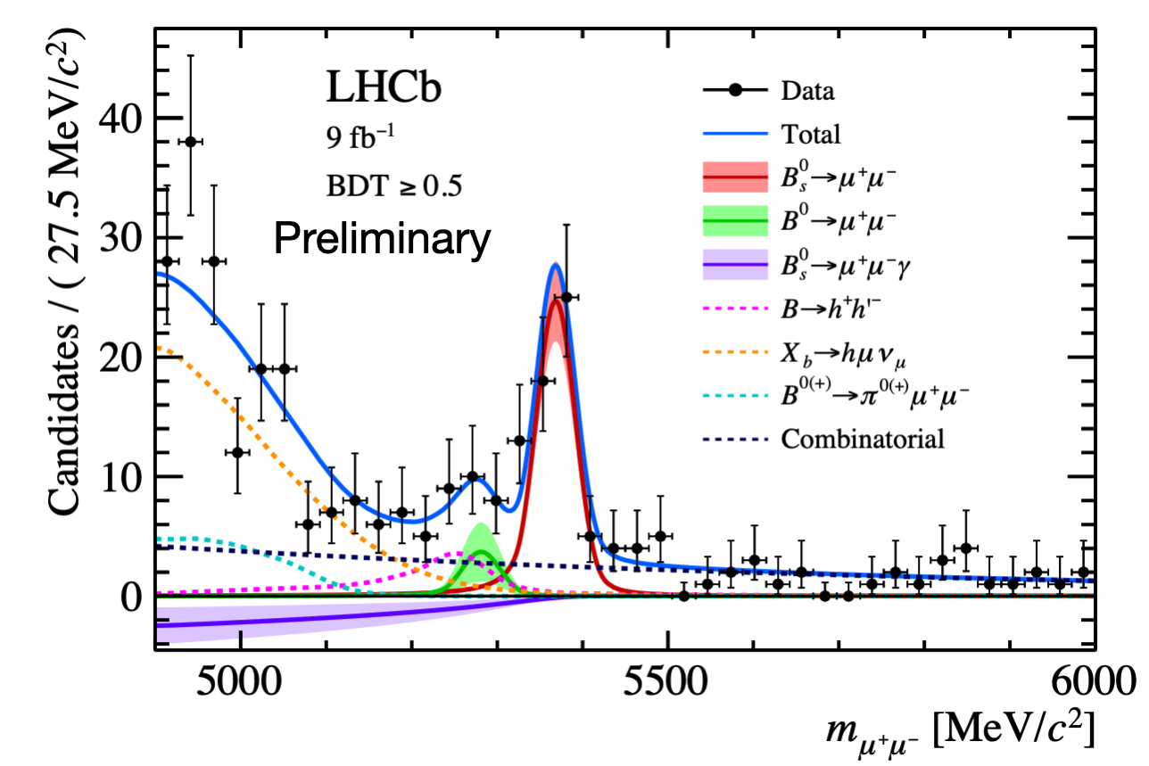
Figure 3: Mass distribution of $B^{0}_{s}\rightarrow\mu^{+}\mu^{-}$, $B^{0}\rightarrow\mu^{+}\mu^{-}$ candidates with BDT $>$ 0.5 in red and green, respectively. The result of the fit is shown in blue and the separated components for the combinatorial and exclusive backgrounds are also detailed.

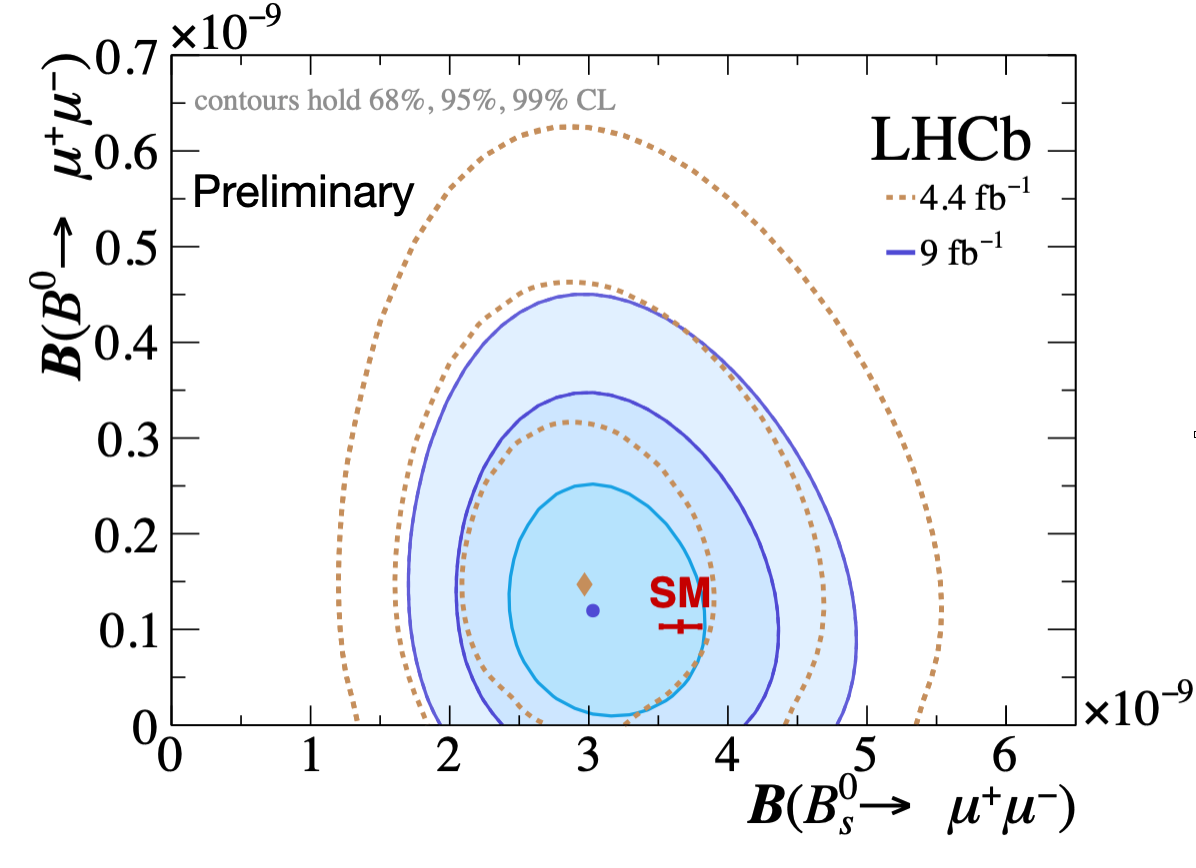
Figure 4: Two dimensional representation of the measured braching fraction values of $B^{0}\rightarrow\mu^{+}\mu^{-}$ and $B^{0}_{s}\rightarrow\mu^{+}\mu^{-}$. The contours of the previous analysis are represented in yellow and the SM value is displayed in red

An important difference with respect to the previous analysis is the addition of the search of $B_{s}^{0}\to\mu^{+}\mu^{-}\gamma$, whose fit component is shown in purple in Fig. 4, a process for which an upper limit on its branching fraction of $\mathcal{B}(B_{s}^{0}\to\mu^{+}\mu^{-}\gamma)_{m_{\mu\mu}>4.9\mbox{ }\mathsf{GeV}/c^{2}}<2.0\times 10^{-9}$ at 95% CL has been established.

3 Conclusion

The latest results for the branching fractions of $B_{(s)}^{0}\to\mu^{+}\mu^{-}$ decays have been presented. The branching fraction of $B_{s}^{0}\to\mu^{+}\mu^{-}$ is determined to be $\mathcal{B}(B_{s}^{0}\to\mu^{+}\mu^{-})=(3.09^{+0.46+0.15}_{-0.43-0.11})\times 10^{-9}$, where the first and second uncertainties correspond to the statistical and systematic uncertainties, respectively. This is the most precise single experiment measurement of the rarest of the B-hadron processes measured so far. An upper limit of $\mathcal{B}(B^{0}\to\mu^{+}\mu^{-})<2.6\times 10^{-10}\mbox{ at 95\% CL}$ is set for the $B^{0}\to\mu^{+}\mu^{-}$ branching fraction, where no significant excess is found. Similarly, an upper limit is found for the $B_{s}^{0}\to\mu^{+}\mu^{-}\gamma$ process of $\mathcal{B}(B_{s}^{0}\to\mu^{+}\mu^{-}\gamma)_{m_{\mu\mu}>4.9\mbox{ }\mathsf{GeV}/c^{2}}<2.0\times 10^{-9}$. All results are consistent with the SM predictions and previous results [9, 10] and help to further constraint NP models.

References

References

- [1] A. J. Buras, [arXiv:hep-ph/9806471 [hep-ph]].
- [2] M. Beneke, C. Bobeth, and R. Szafron, JHEP 10, 232 (2019).
- [3] LHCb collaboration, [arXiv:2103.11769 [hep-ex]].
- [4] K. De Bruyn, R. Fleischer, R. Knegjens, P. Koppenburg, M. Merk, A. Pellegrino and N. Tuning, Phys. Rev. Lett. 109, 041801 (2013).
- [5] R. Fleischer, R. Jaarsma and G. Tetlalmatzi-Xolocotzi, JHEP 05, 156 (2017).
- [6] LHCb collaboration, LHCb-PAPER-2021-007 in preparation.
- [7] LHCb collaboration, LHCb-PAPER-2021-008 in preparation.
- [8] T. Skwarnicki, PhD thesis, Institute of Nuclear Physics, Krakow, 1986, DESY-F31-86-02.
- [9] LHCb collaboration, Phys. Rev. Lett. 118, 191801 (2017).
- [10] ATLAS, CMS and LHCb collaborations, LHCb-CONF-2020-002.