The Kinetic and Hydrodynamic Bohm Criterions
for Plasma Sheath Formation
Masahiro Suzuki1 and Masahiro Takayama2
(1Department of Computer Science and Engineering,
Nagoya Institute of Technology,
Gokiso-cho, Showa-ku, Nagoya, 466-8555, Japan
2Department of Mathematics,
Keio University,
Hiyoshi, Kohoku-ku, Yokohama, 223-8522, Japan
)
Abstract
The purpose of this paper is to mathematically investigate the formation of
a plasma sheath, and to analyze the Bohm criterions which are required for the formation.
Bohm derived originally the (hydrodynamic) Bohm criterion from the Euler–Poisson system.
Boyd and Thompson proposed the (kinetic) Bohm criterion from a kinetic point of view,
and then Riemann derived it from the Vlasov–Poisson system.
In this paper, we prove the solvability of boundary value problems of the Vlasov–Poisson system.
On the process, we see that the kinetic Bohm criterion is a necessary condition for the solvability.
The argument gives a simpler derivation of the criterion.
Furthermore, the hydrodynamic criterion can be derived from the kinetic criterion.
It is of great interest to find the relation between
the solutions of the Vlasov–Poisson and Euler–Poisson systems.
To clarify the relation, we also study the delta mass limit of solutions of the Vlasov–Poisson system.
Keywords:
Vlasov–Poisson system,
Euler–Poisson system,
Boundary value problem,
Delta mass limit.
2020 Mathematics Subject Classification:
35A01, 35M32, 35Q35, 76X05
1 Introduction
The purpose of this paper is to mathematically investigate the formation of
a plasma boundary layer, called as a sheath,
near the surface of materials immersed in a plasma,
and to analyze the Bohm criterions which are required for the formation.
The sheath appears when a material is surrounded
by a plasma and the plasma contacts with its surface.
Because the thermal velocities of electrons are much higher than those of ions,
more electrons tend to hit the material compared with ions.
This makes the material negatively charged with respect to the surrounding plasma.
Then the material with a negative potential attracts and accelerates ions toward the surface,
while repelling electrons away from it.
Eventually, there appears a non-neutral potential region near the surface,
where a nontrivial equilibrium of the densities is achieved.
This non-neutral region is referred as to the sheath.
For more details of physicality of the sheath development,
we refer the reader to [5, 7, 25, 26, 32, 33].
For the formation of sheath, Langmuir [25] observed that
positive ions must enter the sheath region with a sufficiently large flow velocity.
Using the Euler–Poisson system (see (1.5) below),
Bohm [5] proposed the original Bohm criterion
which states that the flow velocity of positive ions at the plasma edge must exceed the ion acoustic speed.
In this paper, we call the criterion a hydrodynamic Bohm criterion.
Nowadays there are many mathematical results
which investigated the sheath formation by using the Euler–Poisson system.
The studies [1, 2, 28, 40, 41, 42] established
the existence and stability of stationary solutions assuming the hydrodynamic Bohm criterion.
These results validated mathematically the criterion.
From different perspectives to the those results’,
the sheath formation was discussed by considering the quasi-neutral limit
as letting the Debye length in the Euler–Poisson system tend to zero [10, 11, 21, 22, 23].
Furthermore, Feldman–Ha–Slemrod [9] studied the sheath formation adopting
a certain hydrodynamic model which describes the dynamics of an interface between the plasma and sheath
(see also [34]).
From a kinetic point of view, Boyd–Thompson [6] proposed a Bohm criterion.
After that Riemann [32] derived it from the Vlasov–Poisson system (see (1.1) below).
We call it a kinetic Bohm criterion in this paper.
There is no mathematical result which investigates the sheath formations
by using the Vlasov–Poisson system with rigorous proofs.
One of our goals is to prove the solvability of boundary value problems of
the Vlasov–Poisson system under the kinetic Bohm criterion.
On the process, we see that the criterion is a necessary condition for the solvability.
The argument gives a simpler derivation of the criterion.
It is worth pointing out that the hydrodynamic Bohm criterion can be derived from the kinetic Bohm criterion.
We are also interested in finding the relation between the solutions of
the Vlasov–Poisson and Euler–Poisson systems.
To clarify the relation, we study some limit of solutions of the Vlasov–Poisson system.
After a suitable nondimensionalization,
the stationary Vlasov–Poisson system is written by
(1.1a)
(1.1b)
where and
are the space variable and velocity, respectively.
The unknown functions and stand
for the velocity distribution of positive ions
and the electrostatic potential, respectively.
The given function denotes the number density of electrons.
We assume that
One of typical functions is the Boltzmann relation .
We study the boundary value problem of (1.1a)–(1.1b) with the boundary conditions
(1.1c)
(1.1d)
(1.1e)
(1.1f)
The constants and
denote the rate of refraction and the voltage on the boundary, respectively.
Furthermore, and are given nonnegative functions.
Physically speaking, the case and corresponds to a completely absorbing wall.
In addition, and mean
that the wall is negatively and positively charged, respectively.
Let us say attractive and repulsive boundaries for positive ions
if and , respectively.
Riemann [32] studied essentially the same boundary value problem as (1.1) to derive the kinetic Bohm criterion
(1.2)
He also assumed that the number density of electrons is given
by a function of the electrostatic potential as in (1.1b).
On the other hand, he did not impose any boundary condition for the potential at ,
and supposed implicitly a situation that is monotone.
The condition (1.1d) is one of simplest boundary conditions that can create the situation.
In stead of (1.1d), we can also impose the following boundary condition:
(1.3)
where is a constant.
This condition means physically that the outgoing fluxes of electrons and ions coincide at the boundary.
Even if we consider a boundary value problem of
(1.1a)–(1.1b) with conditions (1.1c), (1.1e), (1.1f), and (1.3),
it is seen that a value is determined a priori,
and thus we can reduce the problem to the boundary value problem (1.1) (for more details, see Appendix A).
Therefore, we focus ourself on the study of the problem (1.1) in this paper.
The derivation of (1.2) by Riemann [32] is clear to understand, but it seems to be simplified.
Indeed he divided the two cases and ,
and then changed the coordinates according to .
Some expansion of the unknown function was also used.
One of our purposes is to find a simpler derivation
avoiding the use of such coordinate transformations and expansions.
The Vlasov–Poisson system in (1.1)
is given by a system of partial and ordinary differential equations,
while the stationary Euler–Poisson system is given
by a system of just ordinary differential equations.
Besides has a non-local term.
The idea to resolve these difficulties is to reduce the problem (1.1) to
a boundary value problem of a first-order ordinary differential equation only for
by combining the characteristics method and the technique used in [40].
The reduction also enables us to derive more simply the kinetic Bohm criterion (1.2),
which is a necessary condition of the solvability of (1.1).
We will construct the solution under (1.2)
(see Theorems 2.2, 2.5, and 2.6 below).
It is worth pointing out that letting be a delta function
in the kinetic Bohm criterion (1.2), one can obtain
the hydrodynamic Bohm criterion:
(1.4)
where is a positive constant and
means the flow velocity of positive ions at infinite distance.
Bohm derived originally the criterion (1.4) by using
the stationary Euler–Poisson system of cold plasma:
(1.5a)
where , , and
represent the number density and flow velocity of positive ions and
the electrostatic potential, respectively.
Suzuki [40] showed the unique existence of solutions of
the system (1.5a) with the conditions
(1.5b)
where and are constants.
For more details, see Proposition 2.3 below.
It is of great interest to investigate the relation between
the solutions of the Vlasov–Poisson system (1.1)
and the Euler–Poisson system (1.5).
To clarify the relation,
we choose some approximate functions of the delta function for ,
and then show in Theorem 2.4
that the solution of (1.1) converges to that of (1.5)
by taking the limit of approximate functions to the delta function.
We call the limit a delta mass limit.
We review mathematical results on the Vlasov–Poisson system describing the motion of plasma.
For the Cauchy problem, early references [3, 27, 29, 35]
investigated the time-global solvability and dispersive analysis (see also textbooks [12, 31]).
Guo–Strauss [15] established spatially periodic stationary solutions and also investigated its instability
(see also [16] studying the relativistic Vlasov–Maxwell system).
For the the initial–boundary value problem,
Guo [14] and Hwang–Velázquez[20] showed the time-global solvability
adopting the specular reflection boundary condition.
Han-Kwan–Rousset [19] and Han-Kwan–Iacobelli [17, 18]
analyzed the quasi-neutral limit of solutions satisfying a periodic boundary condition.
Furthermore, Skubachevskii [36, 37] and Skubachevskii–Tsuzuki [39]
focused on the analysis of toroidal magnetic plasma containment devices (tokamak),
and established the existence of solutions of the initial–boundary value problem with an external magnetic field,
where supports do not contact with boundaries.
The stationary problem has also been extensively studied.
In an infinite cylinder and a half-space,
Belyaeva [4] and Skubachevskii [38] constructed stationary solutions whose supports do not contact with boundaries by applying an external magnetic field.
Similarly, Knopf [24] established the stationary solution in the whole space,
where the support is contained in an infinite cylinder.
Let us introduce results which treated more similar settings to this paper.
Greengard–Raviart [13] and Rein [30] constructed the stationary solutions
in bounded domains adopting the Dirichlet and the specular refection boundary conditions, respectively.
Recently, Esentürk–Hwang–Strauss [8] showed the solvability of the stationary problem
with diffusive boundary conditions for various domains including a half-space.
For the half-space case, they considered a situation
that there are only particles whose energies are bounded by some finite number,
and the boundary is not electrically charged.
This point is one of the differences between settings in [8] and this paper.
We also emphasize that there is no research
which studies the delta mass limit mentioned above.
This paper is organized as follows.
Section 2 provides our main theorems on the solvability and delta mass limit.
In Section 3, we treat the completely absorbing and attractive boundary, i.e.
and .
Subsection 3.1 is devoted to discussion on a simpler derivation of the kinetic Bohm criterion (1.2).
Subsection 3.2 establishes the solvability of the problem (1.1).
We also justify the delta mass limit in subsection 3.3.
In Section 4, we study general boundaries,
i.e. and .
Before closing this section, we give our notation used throughout this paper.
Notation.
For , is the Lebesgue space
equipped with the norm .
Let us denote by the inner product of .
For and , the function spaces and are defined by
Furthermore, stands for a one-dimensional half space;
stands for a three-dimensional upper half space;
stands for a three-dimensional lower half space.
We also use the one-dimensional indicator function of the set .
2 Main Results
We focus ourself on the analysis of solutions whose potential is monotone,
since the potential is observed as a monotone function when the plasma sheath is formed.
Let us give a definition of solutions of the boundary value problem (1.1).
Definition 2.1.
We say that is a solution of
the boundary value problem (1.1) if it satisfies the following:
(i)
and .
(ii)
, and either or .
(iii)
solves
(2.1a)
(2.1b)
where
.
(iv)
solves (1.1b) with (1.1d) and (1.1f) in the classical sense.
The equation (2.1a) is a standard weak form of the equation (1.1a) and boundary condition (1.1c).
We also remark that it is possible to replace the classical sense in the condition (iv) by the weak sense.
Indeed a weak solution of the problem of (1.1b) with (1.1d) and (1.1f)
is a classical solution if .
Next we discuss some necessary conditions for the solvability of the problem (1.1),
which are used to state our main results.
To solve the Poisson equation (1.1b) with (1.1f),
we must require the quasi-neutral condition
(2.2)
We remark that the boundary value problem (1.1) is overdetermined.
Let us explain briefly for the case .
First must be zero,
and then the equation (1.1a) implies that is independent of .
This fact together with the boundary condition (1.1e) means that .
On the other hand, due to the boundary condition (1.1c),
we have a necessary condition for and :
Consequently, we cannot choose independently and .
For the case , the 111We may not find any physical meaning of (2.3)–(2.5),
but mathematically speaking there is no solution without them.following are necessary conditions:
(2.3)
(2.4)
In particular, for the completely absorbing and attractive boundary, i.e. and , it is written by
(2.5)
We will show that (2.3), (2.4), and (2.5) are necessary conditions in Lemmas 4.1, 4.3, and 3.1, respectively.
From the above observation, we also see that
is a unique solution of (1.1) with ,
and hence suppose hereafter.
We state our main results for the completely absorbing and attractive boundary, i.e.
and in subsection 2.1.
It is one of the most discussed situation in plasma physics.
Subsection 2.2 provides the main results for general boundaries,
i.e. and .
2.1 The Completely Absorbing and Attractive Boundary
We first discuss the results of the solvability of the problem (1.1) with
the completely absorbing and attractive boundary.
After that we also study the delta mass limit of the solution.
It validates rigorously the relation of the kinetic and hydrodynamic Bohm criterions.
The solvability is summarized in Theorem 2.2 below.
Here the set is defined for as
where
(2.6)
The function is well-defined for . Indeed,
(2.7)
Theorem 2.2.
Let and .
Suppose that satisfies and
the necessary conditions (2.2) and (2.5).
(i)
Assume that
(2.8)
Then the set is not empty.
Furthermore, if and only if holds, the problem (1.1) has a unique solution .
There also hold that
(2.9)
(2.10)
where is the one-dimensional indicator function of the set , and
and are positive constants independent of . In addtion, if , then the solution is a classical solution.
(ii)
Assume that
If and only if holds, the problem (1.1) has a unique solution .
Further, (2.9) holds. If , then the solution is a classical solution.
This theorem covers all possible cases of and with ,
and clarifies completely when there is a solution or not.
Assertion (iv) means that the kinetic Bohm criterion (1.2) is a necessary condition for
the solvability of the problem (1.1), since (2.11) is the negation of (1.2).
Assertion (iv) will be shown in subsection 3.1.
The proof gives simultaneously a simpler derivation of the kinetic Bohm criterion than that of [32].
Subsection 3.1 also provides the proof of Assertion (iii).
In subsection 3.2, we will prove Assertions (i) and (ii).
Next we discuss the relation between
the solutions of the Vlasov–Poisson system (1.1)
and the Euler–Poisson system (1.5).
As mentioned in Section 1, the hydrodynamic Bohm criterion (1.4)
can be derived from the kinetic Bohm criterion (1.2)
by plugging a delta function into .
To investigate the relation of solutions,
we use
(2.12)
where is a positive constant and
(2.13)
Note that
This means that converges to the delta function
as .
Let us denote by
the solution of the problem (1.1) with ,
where satisfies
the conditions (2.2), (2.5), and (2.8)
being in Theorem 2.2 for and .
We also introduce the moments
It is expected that the moments converge to of the Euler–Poisson system (1.5)
by taking the delta mass limit as .
The solvability of the problem (1.5) is summarized in the following proposition.
Let (1.4) and hold.
Then the problem (1.5) has a unique monotone solution
.
Furthermore, there hold that
(2.14)
where and are positive constants independent of .
We are now in a position to state our results on the delta mass limit.
Theorem 2.4.
Let , , and .
There exist positive constants and such that if , then the following holds:
(2.15)
for any , where .
Now we mention some remarks.
We cannot choose directly a Maxwellian for due to
the necessary condition (2.5) for the solvability of the problem (1.1),
but it allows products of the Maxwellian and cut-off functions.
For such products, the delta mass limit as corresponds to that
the temperature of the Maxwellian tends to zero.
In this sense, it is reasonable that the limit is a solution of
the Euler–Poisson system of cold plasma.
2.2 General Boundaries
This section provides the main results for general boundary conditions, i.e.
and .
Similarly as Theorem 2.2, we use notation
(2.16)
(2.17)
where
(2.18)
(2.19)
The functions are well-defined for and
with , since all the integrants are nonnegative.
Furthermore, for and , it is seen 333If the problem (1.1) has a solution , then and must hold, whether or not and hold. For more details, see Lemmas 4.1 and 4.3.that
for
(2.20)
for
(2.21)
where is a positive constant, and is a positive constant depending on .
The proofs of the estimates are postponed until Appendix B.
In the definition (2.18), the indicator function is used
to extend continuously beyond .
Now we state main theorems on the solvability by employing the function spaces and . Here the set depends on whereas the set is independent of .
Theorem 2.5.
(Attractive boundary) Let , , 444We can construct multiple solutions for the case , and therefore we exclude it., , and for some .
Suppose 555If a solution exists, then (2.2), (2.3), and must hold. For more details, see Lemma 4.1.that (2.2), (2.3), and hold.
(i)
Assume that .
Then the set is not empty.
Furthermore, 666If for some , the second term in the definition of vanishes for . This means that is independent of . In this case, holds for .if and only if holds, the problem (1.1) has a unique solution .
There also hold that
(2.22)
where and are positive constants independent of .
(ii)
Assume that and .
If and only if holds, the problem (1.1) has a unique solution .
Furthermore, (LABEL:fform2) holds.
(iii)
Assume that and .
Then the problem (1.1) admits no solution.
(iv)
Assume that . Then the problem (1.1) admits no solution.
Theorem 2.6.
(Repulsive boundary) Let , , , and for some .
Suppose 777If a solution exists, then (2.2), (2.4), and must hold.
For more details, see Lemma 4.3.that (2.2), (2.4), and hold.
(i)
Assume that .
Then the set is not empty.
Furthermore, if and only if holds, the problem (1.1) has a unique solution .
There also hold that (2.22) and
(2.23)
(ii)
Assume that and .
If and only if holds, the problem (1.1) has a unique solution .
Furthermore, (2.23) holds.
(iii)
Assume that and .
Then the problem (1.1) admits no solution.
(iv)
Assume that . Then the problem (1.1) admits no solution.
From these theorems, we conclude that
the following conditions are general representations of the kinetic Bohm criterion:
(2.24)
Indeed, it can be rewritten by the kinetic Bohm criterion (1.2)
for the case , , and (for details, see (3.6)).
We can find some functions so that and (2.24) hold,
for example, the functions defined in (2.25) and (2.26) below.
We introduce some more general functions in Appendix C.
Theorems 2.5 and 2.6 will be shown in subsections 4.1 and 4.2, respectively.
We also state the results on the delta mass limit.
Let us define the functions 888
We first determine as (2.26),
and then find a suitable as (2.25)
so that the necessary conditions (2.3) and (2.4) hold.
This choice of is
one of the simplest extensions of in (2.12). and as
(2.25)
(2.26)
where and are defined in (2.13),
and , , , and are constants.
It is supposed that
(2.27)
which ensures (2.2) and for .
Let us denote by
the solution of the problem (1.1) with .
The important thing to note here is that and satisfy
the conditions (2.2)–(2.4) and
being in Theorems 2.5 and 2.6 for the case and .
In this case, is independent of , and also holds,
since the second term in the definition (2.18) of vanishes.
Note that is always independent of .
We also introduce the moments
Theorem 2.7.
Let , , and (2.27) hold.
There exist positive constants , , and such that if
, then the following holds:
(2.28)
for any , where solves a boundary value problem
(2.29a)
(2.29b)
and and are defined as
(2.30)
For the case , i.e. , the functions
in Theorem 2.7 solve a problem
(2.31a)
(2.31b)
which is similar to (1.5).
We conclude that (2.31) is a hydrodynamic model taking the reflection of positive ions
on the boundary into account.
3The Completely Absorbing and Attractive Boundary
In this section, we study the solvability and delta mass limit in Theorems 2.2 and 2.4 for completely absorbing and attractive boundary, i.e. and .
We first show Assertion (iv) in Theorem 2.2 in subsection 3.1.
The proof gives simultaneously a simpler derivation of the kinetic Bohm criterion (1.2) than that of [32],
and also shows that (2.5) is a necessary condition.
In subsection 3.1, we also prove Assertion (iii).
Subsections 3.2 deals with the proofs of Assertions (i) and (ii) of Theorem 2.2.
We show Theorem 2.4 in subsection 3.3.
3.1A Derivation of the Kinetic Bohm Criterion
We discuss necessary conditions for the solvability
by assuming that the solution of the problem (1.1) with and exists.
First we show the following lemma
which ensures immediately Assertion (iv) in Theorem 2.2.
Note that (1.2) is the negation of (2.11).
Lemma 3.1.
Let , , , , and (2.2) hold.
Suppose that the problem (1.1) has a solution .
Then the function satisfies the condition (2.5)
and the kinetic Bohm criterion (1.2).
Furthermore, solves (3.5) below with (1.1d) and (1.1f),
and is written as (2.9) by .
Proof.
First holds thanks to and the condition (ii) in Definition 2.1.
Owing to (1.1f), (2.1b),
, and ,
it follows from (1.1b) that is bounded and therefore is uniformly continuous on .
Then the fact together with (1.1f) and leads to a necessary condition
(3.1)
Let us first show that satisfies (2.5) and is written as (2.9).
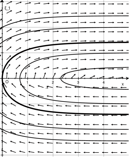
Regarding as a given function and then applying the characteristics method to (2.1a),
we see that the value of must remain a constant along the following characteristic curves:
where is some constant. We draw the illustration of characteristics in Figure 1 below.
Figure 1: characteristic curves for the case
It tells us that
(3.2a)
(3.2b)
(3.2c)
where and
The last inequality (3.2c) means that (2.5) must hold.
Furthermore, we conclude from (3.2) that must be written by (2.9), i.e.
where is the one-dimensional indicator function of the set .
Next we show that satisfies (3.5) below.
Integrating over ,
and using (2.5) and the change of variable ,
we see that
(3.3)
where is the same function defined in (2.6).
Substituting (3.3) into (1.1b) yields an ordinary differential equation for :
(3.4)
Multiply (3.4) by , integrate it over , and use (1.1f) and (3.1) to obtain
(3.5)
where is the same function defined in (2.6).
Thus must satisfy (3.5).
To obtain the kinetic Bohm criterion (1.2),
we divide the proof into two cases and
.
For the former case, follows from the monotone convergence theorem
and the fact .
We also see from (2.2) and (2.5) that
(3.6)
Hence, we arrive at the criterion (1.2) from
(3.5) and (3.6) with the aid of the Taylor theorem.
Furthermore, we show that the other case does not occur.
Suppose that holds.
Then there hold that , , and
where and are some positive constants.
These facts imply that holds for .
It contradicts to (3.5), and thus holds.
Consequently, (1.2) must hold.
∎
This proof provides a simpler derivation of the kinetic Bohm criterion (1.2).
On the other hand, it is clear from (3.5) that the case (a) does not occur.
It suffices to consider the case (b).
Suppose that a solution of the problem (1.1) exists.
For sufficiently large , there exists a sequence such that and .
Then we see from (3.5) that .
This fact contradicts to in Definition 2.1.
Therefore, the problem (1.1) admits no solution.
∎
3.2Solvability
We prove Assertions (i) and (ii) in Theorem 2.2 on the solvability of the problem (1.1).
We first note that (3.6) holds owing to .
It is seen that if (2.8) holds,
since the Taylor theorem with (2.8) and (3.6) ensures that is positive around .
It is easy to see from (3.5) and in Definition 2.1
that the condition is necessary for the solvability stated in Assertions (i) and (ii).
Hereafter we discuss simultaneously Assertions (i) and (ii).
Suppose that holds, which implies that for .
Let us construct with
by solving (3.5) with (1.1d) and (1.1f).
To this end, we rewrite (3.5) into the equivalent equation
(3.7)
The Taylor theorem together with (3.6) and the assumption ensures that
is Lipschitz continuous around .
Combining this and the fact that for ,
we deduce that is Lipschitz continuous on .
Therefore, a standard theory of ordinary differential equations gives
the unique solvability of (3.7) with (1.1d) and (1.1f).
Then it is straightforward to see and
from the equivalent equation.
Thus we have the desired satisfying (3.5) with (1.1d) and (1.1f).
Furthermore, it is easy to show by differentiating (3.5) and using
that satisfies (3.4).
Now we define as (2.9) by using , and prove that satisfies the conditions (i)–(iii) in Definition 2.1.
Owing to (2.5) and , there exists a sequence
such that for , and in as .
Let us show the condition (i), i.e. .
First follows from (2.7) and (3.3).
To investigate the continuity of ,
we set and observe that for ,
Using the change of variable and the fact that holds for ,
we can estimate as
where we have also used the fact in deriving the inequality.
Similarly, as .
Thus and can be arbitrarily small for suitably large .
For the fixed , the dominated convergence theorem ensures that converges to zero as .
Hence, we deduce .
Now it is straightforward to show .
It is clear that the condition (ii), i.e. , holds.
Let us prove (2.1a) and (2.1b) in the condition (iii). Obviously, (2.1b) follows from the same manner as above.
It is also evident that the function defined by replacing by in (2.9) belongs to , and satisfies the weak form (2.1a) for each .
Using the same change of variable as above and letting ,
we see that also satisfies (2.1a).
Consequently, all the conditions (i)–(iii) hold.
The condition (iv) is validated by (2.9), (3.3), and (3.4).
The uniqueness of a solution follows from
the uniqueness of the solution of (3.7) with (1.1d) and (1.1f).
Using (2.5), (2.9), and the fact ,
we can show that
if .
The decay estimate (2.10) follows from (2.8), (3.6), and (3.7). The proof is complete.
∎
For the proof of the delta mass limit as ,
we need to show that in Assertion (i) of Theorem 2.2 is bounded from below
by some positive constant independent of
for the problem (1.1) with .
Here is defined in (2.12).
Corollary 3.2.
Let and .
There exists a positive constant such that
if , then the problem (1.1) with
has a unique solution for any ,
where .
Proof.
We first note that satisfies
the conditions (2.2), (2.5), and (2.8)
being in Theorem 2.2 for any .
It suffices to show that there exists independent of such that
(3.8)
where denotes the function replaced by in (2.6).
Indeed, repeating the proof of Assertions (i) and (ii) of Theorem 2.2 with the aid of (3.8),
we can conclude that the problem (1.1) with
has a unique solution for and
.
Let us complete the proof by showing (3.8).
Using , we observe that
for any , where is independent of .
Recalling (3.6), we also see that
where we have used and .
By the Taylor theorem and the above two inequalities,
we conclude that there exists independent of such that
which together with (3.6) leads to (3.8).
The proof is complete.
∎
3.3The Delta Mass Limit
This section deals with the proof of Theorem 2.4 on the delta mass limit.
Let be a solution in Corollary 3.2,
and also be the moments of .
We first show the estimate of in (2.15).
From (1.5a), (2.14), (3.3), and (3.4),
we observe that
(3.9)
where
Set .
Owing to the assumption , we have .
Then it is seen by taking and small enough that
Furthermore, follows from (1.1f) and (1.5b).
Multiply (3.12) by ,
integrate it over , and use to obtain
(3.13)
The second term on the left hand side is positive.
Indeed, using the mean value theorem, (3.10), and ,
we arrive at
Therefore, (3.13) gives
which means .
Similarly, holds.
Thus the claim (3.11) is vaild.
Next let us estimate by as
where we have used the fact in deriving the equality,
and is a positive constant independent of .
This together with (3.11) leads to the estimate of in (2.15).
We complete the proof by showing the other estimates in (2.15).
Let us first handle .
It is clear that holds owing to (3.3).
With the aid of this and (2.14), we estimate as
Let us treat .
By the change of variable , the term is rewritten as
In this section, we prove Theorems 2.5–2.7
on the solvability and delta mass limit for general boundaries.
Subsections 4.1 and 4.2 deal with the solvability for
the attractive and repulsive boundaries, respectively.
In subsection 4.3, we study the delta mass limit.
4.1Solvability for the Attractive Boundary
We start from studying the necessary conditions for the solvability of the problem (1.1)
similarly as in Section 3.
Specifically, we show the following lemma which ensures immediately Assertion (iv) in Theorem 2.5.
Lemma 4.1.
Let , , , , , , and (2.2) hold.
Suppose that the problem (1.1) has a solution .
Then , , and the function satisfies the condition (2.3).
Furthermore, solves (4.4) below with (1.1d) and (1.1f),
and is written as (LABEL:fform2) by .
If , the generalized Bohm criterion holds:
(4.1)
Proof.
In much the same way as in the proof of Lemma 3.1, we see
and .
Let us first show that satisfies (2.3) and is written by (LABEL:fform2).
Applying the characteristics method to (2.1a),
we see that the value of must remain a constant along the characteristic curves
,
where is some constant.
The characteristics are drawn as in Figure 1.
Therefore, there hold that
where and
The last equality means that (2.3) must hold.
Furthermore, we conclude from these three equalities 999If and , we have multiple choices for the second term on the right hand side of (LABEL:fform2).that must be written by (LABEL:fform2), i.e.
Next we show that satisfies (4.4) below.
Integrating (LABEL:fform2) over and using
the change of variables , , and
for the first, second, and third terms on the right hand side of (LABEL:fform2), respectively, we see that
(4.2)
where and is the same function defined in (2.18).
Substituting (4.2) into (1.1b) yields an ordinary differential equation for :
(4.3)
Multiply (4.3) by , integrate it over , and use (1.1f) and to obtain
(4.4)
where the function is the same function defined in (2.16).
Thus must satisfy (4.4).
Now we show which immediately gives .
Owing to in Definition 2.1 and (2.1b), there hold that
These imply with the aid of (1.1f),
, and in Definition 2.1.
What is left is to obtain the generalized Bohm criterion (4.1).
We see from and (2.2) that
(4.5)
If , we arrive at (4.1)
from (4.4) and (4.5) with the aid of the Taylor theorem.
The proof is complete.
∎
Assertion (iii) in Theorem 2.5 can be shown
by the same method as in the proof of Assertion (iii) in Theorem 2.2 with the aid of (4.4).
We omit the proof.
Let us show Assertions (i) and (ii) in Theorem 2.5.
We first note that (4.5) holds. It is seen that if ,
since the Taylor theorem with (4.5) ensures that is positive around .
Let us show that is a necessary condition for the solvability stated in Assertions (i) and (ii).
Suppose that a solution exists for .
Then and .
Furthermore, there exists a unique so that .
On the other hand, due to (4.4), it is seen that . This contradicts to in Definition 2.1.
Hence, is necessary.
Hereafter we discuss simultaneously Assertions (i) and (ii).
Suppose that holds, which implies that for .
The Taylor theorem with (4.5) and the assumption ensures that
is Lipschitz continuous around .
Combining this and the fact that for ,
we deduce that is Lipschitz continuous on .
Hence, we can define by solving (4.4) with (1.1d) and (1.1f).
Then it is seen that satisfies , , and (4.3) by following the proof of Assertions (i) and (ii) of Theorem 2.2 in subsection 3.2.
Now by using , we define as (LABEL:fform2), i.e.
and prove that satisfies the conditions (i)–(iii) in Definition 2.1.
Owing to (2.3), , and ,
there exist sequences
such that (2.3) with holds;
holds for ; holds for ;
in as ;
in as .
Let us show the condition (i), i.e. .
It is seen that
in much the same way as the proof of Assertions (i) and (ii) of Theorem 2.2.
The fact follows from (2.20) and (4.2).
To investigate the continuity of , we set and observe that for ,
Using the change of variable , we can estimate as
where is the Hölder conjugate of , and is some positive constant. Similarly, as .
Thus and can be arbitrarily small for suitably large .
For the fixed , the dominated convergence theorem ensures that converges to zero as .
Hence, we deduce that holds and so does
.
Now it is straightforward to show .
It is clear that the condition (ii), i.e. , holds.
Let us prove (2.1a) and (2.1b) in the condition (iii).
Obviously, (2.1b) follows from the same manner as above.
It is also evident that the function defined by replacing by in (LABEL:fform2) belongs to , and satisfies the weak form (2.1a) for each .
Letting , we see that also satisfies (2.1a).
Consequently, all the conditions (i)–(iii) hold.
The condition (iv) is validated by (LABEL:fform2), (4.2), and (4.3).
The uniqueness of a solution follows from
the uniqueness of the solution of (4.4) with (1.1d) and (1.1f).
We have the decay estimate (2.22) from (4.4), (4.5), and
. The proof is complete.
∎
We also have Corollary 4.2 stating
that in Assertion (i) of Theorem 2.5 is bounded from below
by some positive constant independent of and
for the problem (1.1) with ,
where and are defined in (2.25) and (2.26).
As mentioned just after (2.27), the functions and satisfy
the conditions (2.2), (2.3), and being in Theorem 2.5 for and provided that (2.27) holds. Furthermore, is independent of , and also holds for .
We omit the proof of Corollary 4.2, since it is the same as the proof of Corollary 3.2.
Corollary 4.2.
Let and (2.27) hold.
There exist positive constants and such that
if , then the problem (1.1) with
has a unique solution for any .
4.2 Solvability for the Repulsive Boundary
We first study the necessary conditions for the solvability of the problem (1.1)
similarly as in subsection 4.1.
Specifically, we show the following lemma which ensures immediately Assertion (iv) in Theorem 2.6.
Lemma 4.3.
Let , , , , , and (2.2) hold.
Suppose that the problem (1.1) has a solution .
Then , , and the function satisfies the condition (2.4).
Furthermore, solves (4.9) below with (1.1d) and (1.1f),
and is written as (2.23) by .
If , the generalized Bohm criterion also holds:
(4.6)
Proof.
In the same manner as in subsection 3.1, we see
and .
Let us first show that satisfies (2.4) and is written by (2.23).
Applying the characteristics method to (2.1a),
we see that the value of must remain a constant along the characteristic curves
,
where is some constant.
We draw the illustration of characteristics in Figure 2 below.
Figure 2: characteristics curves for the case
It tells us that
where
The second and third equalities mean that (2.4) must hold.
Furthermore, we conclude from these three equalities that must be written by (2.23), i.e,
Next we show that satisfies (4.9) below.
Integrating (2.23) over and
using the change of variables and
for the first and second terms of the right hand side of (2.23), respectively,
we see that
(4.7)
where is the same function defined in (2.19).
Substituting (4.7) into (1.1b) yields an ordinary differential equation for :
(4.8)
Multiply (4.8) by , integrate it over , and use (1.1f) and to obtain
(4.9)
where the function is the same function defined in (2.17).
Thus must satisfy (4.9).
Now we show which immediately gives .
Owing to and (2.1b) in Definition 2.1, there hold that
These imply with the aid of (1.1f),
, and in Definition 2.1.
What is left is to obtain the generalized Bohm criterion (4.6).
We see from and (2.2) that
(4.10)
If , we arrive at (4.6)
from (4.9) and (4.10) with the aid of the Taylor theorem.
The proof is complete.
∎
Assertion (iii) in Theorem 2.6 can be shown
by the same method as in the proof of Assertion (iii) in Theorem 2.2 with the aid of (4.9).
We omit the proof.
Let us show Assertions (i) and (ii) in Theorem 2.6.
In the same way as in the proof of Assertions (i) and (ii) in Theorem 2.5,
we first see that if ;
is necessary;
is Lipschitz continuous on .
To find a solution with of the equation (4.9) with (1.1d) and (1.1f),
we rewrite (4.9) into the equivalent equation
Then we complete the proof in the same manner as that of Assertions (i) and (ii) of Theorems 2.2 and 2.5.
∎
Similarly as the proof of Corollary 3.2,
we also see that in Assertion (i) of Theorem 2.6 is bounded from above
by some negative constant independent of
for the problem (1.1) with .
Here and defined in (2.25) and (2.26) satisfy
the conditions (2.2), (2.4), and being
in Theorem 2.6 for and provided that (2.27) holds.
The result is summarized in the following corollary.
Corollary 4.4.
Let (2.27) hold.
There exist positive constants and such that
if , then the problem (1.1) with
has a unique solution for any .
4.3 The Delta Mass Limit
This section provides the proof of Theorem 2.7 on the delta mass limit.
We start from showing the next lemma on the solvability of the problem (2.29).
Lemma 4.5.
Let (2.27) hold.
There exists a positive constant such that
if , then the problem (2.29) has a unique monotone solution .
Proof.
We first note that must hold if such a solution exists.
Now multiply (2.29a) by and integrate it over to obtain
It is straightforward to see that holds for some .
From , , and (2.27), one can know that
Then following the proofs of Assertions (i) and (ii) of Theorems 2.2, 2.5, and 2.6, we can complete the proof.
∎
Let be solutions in Corollaries 4.2 and 4.4,
and also be the moments of .
We first show the estimate of in (2.28).
From (2.29a), (4.3), and (4.8), we observe that
where we have used the fact that the second term vanishes in (2.20) for and ,
and and are defined as
Set .
Owing to and (2.27), we have .
Then it is seen by taking and small enough that
where we have used the fact
in deriving the equality,
and is a positive constant independent of .
This together with (4.11) leads to the estimate of in (2.28).
We complete the proof by showing the other estimates in (2.28).
It is clear that holds owing to (4.2) and (4.7).
We estimate as
Let us treat .
By the change of variables ,
the term is rewritten as
Acknowledge.
This work was supported by JSPS KAKENHI Grant Numbers 18K03364 and 21K03308.
Appendix A Reduction
In this section, we reduce the boundary value problem of
(1.1a)–(1.1b) with conditions (1.1c), (1.1e), (1.1f), and (1.3)
to the boundary value problem (1.1).
For simplicity, we treat the reduction only for the completely absorbing boundary, i.e. .
Suppose that the former boundary value problem has a solution with .
It is sufficient to show that a value is determined a priori by .
Indeed we can construct the soluiton of the former problem by solving
the problem (1.1) with .
Let us find an a priori value .
Following the proof of Lemma 3.1,
we see that must be written by the form (2.9) even for the former problem.
Substituting (2.9) into (1.3) with yields the 101010If there is no value so that this condition holds, the boundary value problem of
(1.1a)–(1.1b) with conditions (1.1c), (1.1e), (1.1f), and (1.3) admits no solution.following condition:
By solving this with respect to , we can know the a priori value .
Consequently, the former problem can be reduced to
the problem (1.1) with .
Appendix B Estimates of
This section provides the proofs of estimates (2.20) and (2.21).
First we can obtain (2.20) by using the Hölder inequality as follows:
for , where is the Hölder conjugate of . Similarly, we observe that for ,
We investigate properties of the functions defined in (2.16) and (2.17).
Lemma C.1.
(Attractive boundary) Let , , and satisfy and
(C.1)
for some .
Suppose that satisfies , (2.2), (2.3), and (2.8).
Then there exists a positive constant such that if ,
the function belongs to and satisfies .
(Repulsive boundary) Let , , and .
Suppose that satisfies , (2.2), (2.4), (2.8), and
for some .
Then there exists a constant such that if ,
the function belongs to and satisfies .
Proof.
We show only the assertion for the attractive boundary, since the other one can be shown similarly.
Recalling the definition of in (2.18),
we see from (C.1) that the second term vanishes for sufficiently small .
Therefore, we can complete the proof
by following the same argument as in the last paragraph of the proof of Lemma 3.1,
and also noting that
where we have used (2.8) in deriving the last inequality.
∎
References
[1]A. Ambroso,
Stability for solutions of a stationary Euler–Poisson problem,
Math. Models Methods Appl. Sci. 16 (2006), 1817–1837.
[2]A. Ambroso, F. Méhats and P.-A. Raviart,
On singular perturbation problems for the nonlinear Poisson equation,
Asympt. Anal. 25 (2001), 39–91.
[3]C. Bardos and P. Degond,
Global existence for the Vlasov–Poisson equation in 3 space variables with small initial data,
Ann. Inst. H. Poincaré Anal. Non Linéaire 2 (1985), 101–118.
[4]Y. O. Belyaeva,
Stationary solutions of the Vlasov–Poisson system for two-component plasma
under an external magnetic field in a half-space,
Math. Model. Nat. Phenom. 12 (2017), 37–50.
[5]D. Bohm,
Minimum ionic kinetic energy for a stable sheath,
in The characteristics of electrical discharges in magnetic fields,
A. Guthrie and R.K.Wakerling eds., McGraw-Hill, New York, (1949), 77–86.
[6]R. L. F. Boyd and J. B. Thompson,
The Operation of Langmuir Probes in Electro-Negative Plasmas,
Proc. R. Soc. Lond. A 252 (1959), 102–119.
[7]F. F. Chen,
Introduction to Plasma Physics and Controlled Fusion,
2nd edition edition, Springer, 1984.
[8]E. Esentürk, H. J. Hwang, and W. A. Strauss,
Stationary solutions of the Vlasov–Poisson system with diffusive boundary conditions,
J. Nonlinear Sci. 25 (2015), 315–342.
[9]M. Feldman, S.-Y. Ha, and M. Slemrod,
A geometric level-set formulation of a plasma-sheath interface,
Arch. Ration. Mech. Anal. 178 (2005), 81–123.
[10]D. Gérard-Varet, D. Han-Kwan, and F. Rousset,
Quasineutral limit of the Euler–Poisson system for ions
in a domain with boundaries,
Indiana Univ. Math. J. 62 (2013), 359–402.
[11]D. Gérard-Varet, D. Han-Kwan, and F. Rousset,
Quasineutral limit of the Euler–Poisson system for ions
in a domain with boundaries II,
J. Éc. polytech. Math. 1 (2014), 343–386.
[12]R. T. Glassey,
The Cauchy problem in kinetic theory, Society for Industrial and Applied Mathematics (SIAM),
Philadelphia, PA, 1996.
[13]C. Greengard and P.-A. Raviart,
A boundary value problem for the stationary Vlasov–Poisson equations: The plane diode,
Comm. Pure Appl. Math. 43 (1990), 473–507.
[14]Y. Guo,
Regularity for the Vlasov equations in a half space,
Indiana Univ. Math. J. 43 (1994), 255–320.
[15]Y. Guo and W. Strauss,
Instability of periodic BGK equilibria,
Comm. Pure Appl. Math. 48 (1995), 861–894.
[16]Y. Guo and W. Strauss,
Unstable BGK solitary waves and collisionless shocks,
Comm. Math. Phys. 195 (1998), 267–293.
[17]D. Han-Kwan and M. Iacobelli,
Quasineutral limit for Vlasov–Poisson via Wasserstein stability estimates in higher dimension,
J. Differential Equations 263 (2017), 1–25.
[18]D. Han-Kwan and M. Iacobelli,
The quasineutral limit of the Vlasov–Poisson equation in Wasserstein metric,
Commun. Math. Sci. 15 (2017), 481–509.
[19]D. Han-Kwan and F. Rousset,
Quasineutral limit for Vlasov–Poisson with Penrose stable data,
Ann. Sci. Éc. Norm. Supér. 49 (2016), 1445–1495.
[20]H. J. Hwang and J. J. L. Velázquez,
On global existence for the Vlasov–Poisson system in a half space,
J. Differential Equations 247 (2009), 1915–1948.
[21]C.-Y. Jung, B. Kwon, and M. Suzuki,
Quasi-neutral limit for the Euler–Poisson system in the presence of plasma sheaths with spherical symmetry,
Math. Models Methods Appl. Sci. 26 (2016), 2369–2392.
[22]C.-Y. Jung, B. Kwon, and M. Suzuki,
Quasi-neutral limit for Euler–Poisson system in the presence of boundary layers in an annular domain,
J. Differential Equations 269 (2020), 8007–8054.
[23]C.-Y. Jung, B. Kwon, and M. Suzuki,
On approximate solutions to the Euler–Poisson system with boundary layers,
Commun. Nonlinear Sci. Numer. Simul. 96 (2021), 105717.
[24]P. Knopf,
Confined steady states of a Vlasov–Poisson plasma in an infinitely long cylinder,
Math. Methods Appl. Sci. 42 (2019), 6369–6384.
[25]I. Langmuir,
The interaction of electron and positive ion space charges in cathode sheaths,
Phys. Rev. 33 (1929), 954–989.
[26]M. A. Lieberman and A. J. Lichtenberg,
Principles of Plasma Discharges and Materials Processing,
2nd edition, Wiley-Interscience, 2005.
[27]P.-L. Lions and B. Perthame,
Propagation of moments and regularity for the 3-dimensional Vlasov–Poisson system,
Invent. Math. 105 (1991), 415–430.
[28]S. Nishibata, M. Ohnawa, and M. Suzuki,
Asymptotic stability of boundary layers
to the Euler–Poisson equations arising in plasma physics,
SIAM J. Math. Anal. 44 (2012), 761–790.
[29]K. Pfaffelmoser,
Global classical solutions of the Vlasov–Poisson system in three dimensions for general initial data,
Journal of Differential Equations 95 (1992), 281–303.
[30]G. Rein,
Existence of stationary, collisionless plasmas in bounded domains,
Math. Methods Appl. Sci. 15 (1992), 365–374.
[31]G. Rein,
Collisionless kinetic equations from astrophysics—the Vlasov–Poisson system,
Handbook of differential equations: evolutionary equations, Vol. III, 383–476, Handb. Differ. Equ., Elsevier/North-Holland, Amsterdam, 2007.
[32]K.-U. Riemann,
The Bohm criterion and sheath formation,
J. Phys. D: Appl. Phys. 24 (1991), 493–518.
[33]K.-U. Riemann,
The Bohm Criterion and Boundary Conditions for a Multicomponent System,
IEEE Trans. Plasma Sci. 23 (1995), 709–716.
[34]K.-U. Riemann and T. Daube,
Analytical model of the relaxation of a collisionless ion matrix sheath,
J. Appl. Phys. 86 (1999), 1201–1207.
[35]J. Schaeffer,
Global existence of smooth solutions to the Vlasov–Poisson system in three dimensions,
Communications in Partial Differential Equations 16 (1991), 1313–1335.
[36]A. L. Skubachevskii,
On the unique solvability of mixed problems for the system of Vlasov–Poisson equations in a half-space,
Dokl. Math. 85 (2012), 255–258.
[37]A. L. Skubachevskii,
Initial–Boundary Value Problems for the Vlasov–Poisson equations in a half-space,
Proc. Steklov Inst. Math. 283 (2013), 197–225.
[38]A. L. Skubachevskii,
Vlasov–Poisson equations for a two-component plasma in a homogeneous magnetic field,
Russ. Math. Surv. 69 (2014), 291–330.
[39]A. L. Skubachevskii and Y. Tsuzuki,
Classical solutions of the Vlasov–Poisson equations with external magnetic field in a half-space,
Comput. Math. Math. Phys., 57 (2017), 541–557.
[40]M. Suzuki,
Asymptotic stability of stationary solutions
to the Euler–Poisson equations arising in plasma physics,
Kinet. Relat. Models 4 (2011), 569–588.
[41]M. Suzuki,
Asymptotic stability of a boundary layer
to the Euler–Poisson equations for a multicomponent plasma,
Kinet. Relat. Models 9 (2016), 587–603.
[42]M. Suzuki and M. Takayama,
Stability and existence of stationary solutions to the Euler–Poisson equations in a domain with a curved boundary,
Arch. Ration. Mech. Anal. 239 (2021), 357–387.