Group Testing under Superspreading Dynamics

Abstract

Testing is recommended for all close contacts of confirmed COVID-19 patients. However, existing group testing methods are oblivious to the circumstances of contagion provided by contact tracing. Here, we build upon a well-known semi-adaptive pool testing method, Dorfman’s method with imperfect tests, and derive a simple group testing method based on dynamic programming that is specifically designed to use the information provided by contact tracing. Experiments using a variety of reproduction numbers and dispersion levels, including those estimated in the context of the COVID-19 pandemic, show that the pools found using our method result in a significantly lower number of tests than those found using standard Dorfman’s method, especially when the number of contacts of an infected individual is small. Moreover, our results show that our method can be more beneficial when the secondary infections are highly overdispersed.

Introduction

As countries around the world learn to live with COVID-19, the use of testing, contact tracing and isolation (TTI) has been proven to be as important as social distancing for containing the spread of the disease [1]. However, as the infection levels grow, TTI reaches a tipping point and its effectiveness quickly degrades as the health authorities lack resources to trace and test all contacts of diagnosed individuals [2]. In this context, there has been a flurry of interest on the use of group testing—testing groups of samples simultaneously—to scale up testing under limited resources.

The literature on group testing methods has a rich history, starting with the seminal work by Dorfman [3, 4, 5]. However, existing methods [6, 7], including those developed and used in the context of the COVID-19 pandemic [8, 9, 10, 11, 12, 13, 14, 15, 16], are oblivious to the circumstances of contagion provided by contact tracing and assume statistical independence of the samples to be tested. This assumption can be seemingly justified by classical epidemiological models where the number of infections caused by a single individual follows a Poisson distribution. However, in COVID-19, there is growing evidence suggesting that the number of secondary infections caused by a single individual is overdispersed—most individuals do not infect anyone but a few superspreaders infect many in infection hotspots [17, 18, 19, 20, 21, 22, 23]. Overdispersion has been also observed in MERS and SARS [24, 25, 26]. In this work, our goal is to develop group testing methods that are specifically designed to use the information provided by contact tracing and are effective in the presence of overdispersion.

More specifically, we build upon a well-known semi-adaptive pool testing method, Dorfman’s method with imperfect tests [27, 5]. In Dorfman’s method, samples from multiple individuals are first pooled together and evaluated using a single test. If a pooled sample is negative, all individuals in the pooled sample are deemed negative. If the pooled sample is positive, each individual sample from the pool is then tested independently. However, rather than modeling the probability that each individual sample is positive using an independent Bernoulli distribution as in Dorfman’s method, we assume that: (i) the samples to be tested are all the contacts of a diagnosed individual during their infectious period, who are identified using contact tracing, and (ii) the number of true positive samples, i.e., secondary infections by the diagnosed individual, follows an overdispersed negative binomial distribution [22, 23]. Given any arbitrary set of pools, we then compute the average number of tests and the expected number of false negatives and false positives under our model. Finally, we introduce a dynamic programming algorithm to efficiently find the set of pools that optimally trade off the average number of tests, false negatives and false positives in polynomial time. Experiments using a variety of reproduction numbers and dispersion levels in secondary infections, including those observed for COVID-19, show that the pools found using our method result in a significantly lower average number of tests than those found using standard Dorfman’s method, especially when the number of contacts of an infected individual is small. Moreover, our results show that our method can be particularly beneficial when the number of secondary infections caused by an infectious individual is highly overdispersed.

Methods

Modeling overdispersion of infected contacts

Previous work have mostly built on the assumption that the number of infections $X$ caused by a single individual follows a Poisson distribution with mean $r$, so $X\sim\text{Pois}(r)$, where $r$ is often called the effective reproduction number. However, having equal mean and variance, the Poisson is unable to capture settings where the number of cases to be tested for exhibits higher variance. Following recent work in the context of COVID-19 [19, 22], we instead model $X$ using a generalized negative binomial distribution. For a (standard) negative binomial distribution, $X\sim\text{NBin}(k,p)$ can be interpreted as the number of successes before the $k$-th failure in a sequence of Bernoulli trials with success probability $p$. For a generalized negative binomial distribution, $k>0$ can take real values and the probability mass function is given by

$$P(X=n) =\frac{\Gamma(n+k)}{\Gamma(k)n!}p^{n}(1-p)^{k},$$

where $k$ is called the dispersion parameter and parameterizes higher variance of the distribution for small $k$. Since $\mathbb{E}[X]=kp/(1-p)$, we assume in this work that the number of secondary infections $X$ is distributed as $X\sim\text{NBin}\left(k,p\right)$ with $p=r/(k+r)$, hence parameterizing $X$ via its mean $\mathbb{E}[X]=r$ and dispersion parameter $k$. Under this parameterization, $\text{Var}[X]=r(1+r/k)$, which is greater than the variance of the Poisson $r$ for $k<\infty$. For $k\rightarrow\infty$, the sequence of random variables $X_{k}\sim\text{NBin}(k,r/(k+r))$ converges in distribution to $X\sim\text{Pois}(r)$, making the negative binomial a suitable generalization of the Poisson for modeling secondary infections.

Assuming we test all contacts of a diagnosed individual during their infectious period, we have prior information about the maximum number of possible infections $N$ in practice. In this setting, we will write

$$q_{r,k,N}(n):=P(X=n\,|\,X\leq N)\quad\text{when}\quad X\sim\text{NBin}\left(k,r/(k+r)\right).$$ (1)

Here, note that $P(X=n\,|\,X\leq N)=P(X=n)/P(X\leq N)$ if $n\leq N$ and 0 otherwise.

Pooling contacts of a positively diagnosed individual

In this context, our goal is to identify infected individuals among all contacts $\mathcal{N}$ of a positively diagnosed individual via testing, where $|\mathcal{N}|=N$. For events concerning each individual $j\in\mathcal{N}$, we define the following indicator random variable:

$$I_{j} ={\mathbbm{1}[\text{individual $j$ is infected}]}$$

In addition, for each pool of individuals ${\mathcal{S}}\subseteq\mathcal{N}$, we define the number of infected in ${\mathcal{S}}$ as $I({\mathcal{S}}):=\sum_{j\in{\mathcal{S}}}I_{j}$. Following our assumption on the distribution of the number of secondary infections, we define

$$P(I(\mathcal{N})=n)=q_{r,k,N}(n)$$

Let $T({\mathcal{S}})={\mathbbm{1}[\text{test of pool ${\mathcal{S}}$ is positive}]}$. To account for the sensitivity $s_{e}$ (i.e., true positive probability) and specificity $s_{p}$ (i.e., true negative probability) of tests, we parameterize the conditional probabilities as

$$P(T({\mathcal{S}})=1\,|\,I({\mathcal{S}})>0) =s_{e}$$

$$P(T({\mathcal{S}})=0\,|\,I({\mathcal{S}})=0) =s_{p}$$

In the above, following the literature on the group testing [5], we assume that the sensitivity of pool tests is independent of the exact number of infected individuals in the pool. Moreover, while dilution has been shown to often be negligible [28], the effect can easily be addressed by making the conditional $T({\mathcal{S}})\,|\,I({\mathcal{S}})$, dependent on the corresponding pool size $|{\mathcal{S}}|$.

Dorfman testing under overdispersion of infected contacts

Dorfman testing proceeds by pooling individuals into non-overlapping partitions of $\mathcal{N}$ and first testing the combined samples of each pool using a single test. Every member of a pool is marked as negative if their combined sample is negative. If a combined sample of a pool is positive, each individual of the pool is subsequently tested individually to determine who exactly is marked positive in the pool.

Let $D^{{\mathcal{S}}}_{j}$ denote the indicator random variable for the event that individual $j$ is marked as infected in pool ${\mathcal{S}}\subseteq\mathcal{N}:|{\mathcal{S}}|>1$ after Dorfman testing. Then, $D^{{\mathcal{S}}}_{j}$ can be expressed as

$$D^{{\mathcal{S}}}_{j} ={\mathbbm{1}[T({\mathcal{S}})=1\cap T(\{j\})=1]},$$

i.e., taking value 1 if and only if the combined sample of pool ${\mathcal{S}}$ is first tested positive and the sample of individual $j$ is tested positive in the second step. In the simple case of $|{\mathcal{S}}|=1$, we have $D^{{\mathcal{S}}}_{j}=T(\{j\})$.

Expected number of tests

Let $K({\mathcal{S}})$ be the number of tests performed when testing pool ${\mathcal{S}}$ as described above. Then, the expected number of tests $\mathbb{E}[K({\mathcal{S}})]$ due to a pool ${\mathcal{S}}$ is:

$$\mathbb{E}[K({\mathcal{S}})] =\begin{cases}1+f({\mathcal{S}})&|{\mathcal{S}}|>1\\ 1&|{\mathcal{S}}|=1\end{cases}$$

where $f({\mathcal{S}})$ is given by

$$f({\mathcal{S}}) =|S|\Big{[}1-P\big{(}T({\mathcal{S}})=0\big{)}\Big{]}$$

$$=|S|\Bigg{[}1-\sum_{s=0}^{|{\mathcal{S}}|}P\big{(}T({\mathcal{S}})=0\,|\,I({\mathcal{S}})=s\big{)}P\big{(}I({\mathcal{S}})=s\big{)}\Bigg{]}$$

$$=|S|\Bigg{[}1-\sum_{s=1}^{|{\mathcal{S}}|}P\big{(}T({\mathcal{S}})=0\,|\,I({\mathcal{S}})=s\big{)}\sum_{n=s}^{N}P\big{(}I({\mathcal{S}})=s\,|\,I(\mathcal{N})=n\big{)}P\big{(}I(\mathcal{N})=n\big{)}$$

$$\quad\quad\quad-P\big{(}T({\mathcal{S}})=0\,|\,I({\mathcal{S}})=0\big{)}\sum_{n=0}^{N}P\big{(}I({\mathcal{S}})=0\,|\,I(\mathcal{N})=n\big{)}P\big{(}I(\mathcal{N})=n\big{)}\Bigg{]}$$

$$=|S|\Bigg{[}1-\sum_{s=1}^{|{\mathcal{S}}|}(1-s_{e})\sum_{n=s}^{N}\frac{\binom{n}{s}\binom{N-n}{|{\mathcal{S}}|-s}}{\binom{N}{|{\mathcal{S}}|}}q_{r,k,N}(n)-s_{p}\sum_{n=0}^{N}\frac{\binom{N-n}{|{\mathcal{S}}|}}{\binom{N}{|{\mathcal{S}}|}}q_{r,k,N}(n)\Bigg{]}$$

where the last step follows from the fact that $I({\mathcal{S}})\,|\,I(\mathcal{N})=n\sim\text{HGeom}(N,n,|{\mathcal{S}}|)$, our assumption about $\mathbb{P}(I(\mathcal{N})=n)$ and our assumptions about $T({\mathcal{S}})$.

Expected number of false negatives

To compute the number of false negatives, we distinguish between two cases. If $|{\mathcal{S}}|=1$, i.e., the pool consists of only one person, there is no distinction between a group test and an individual test. Therefore, a false negative can occur only if the person is infected and the test turns out negative. Thus,

$$\mathbb{E}[FN({\mathcal{S}})]=(1-s_{e})P(I({\mathcal{S}})=1)=(1-s_{e})\sum_{n=1}^{N}\frac{n}{N}q_{r,k,N}(n)$$

If $|{\mathcal{S}}|>1$, a pooled test is performed and, if it turns out positive, individual tests are performed afterwards. The expected number of false negatives in this case is

$$\mathbb{E}[FN({\mathcal{S}})]=\sum_{s=1}^{|{\mathcal{S}}|}s\,P(T({\mathcal{S}})=0\,|\,I({\mathcal{S}})=s)P(I({\mathcal{S}})=s)+\sum_{s=1}^{|{\mathcal{S}}|}P(T({\mathcal{S}})=1\,|\,I({\mathcal{S}})=s)P(I({\mathcal{S}})=s)\,s\,(1-s_{e})$$

where the first term corresponds to the case where the group test outcome is falsely negative and the second term corresponds to the case where the group test outcome is truly positive and the individual tests are falsely negative. Using our assumptions about the individual probabilities, we can rewrite the above expression as

$$\mathbb{E}[FN({\mathcal{S}})]=\sum_{s=1}^{|{\mathcal{S}}|}s(1-s_{e})P(I({\mathcal{S}})=s)+\sum_{s=1}^{|{\mathcal{S}}|}s(1-s_{e})s_{e}P(I({\mathcal{S}})=s)=\sum_{s=1}^{|{\mathcal{S}}|}s(1-s_{e}^{2})\left[\sum_{n=s}^{N}\frac{\binom{n}{s}\binom{N-n}{|{\mathcal{S}}|-s}}{\binom{N}{|{\mathcal{S}}|}}q_{r,k,N}(n)\right]$$

Expected number of false positives

We likewise distinguish between the two cases for computing the number of false positives. Again, if $|{\mathcal{S}}|=1$, there is no distinction between a group test and an individual test. Therefore, a false positive can occur only if the person is not infected and the test turns out positive. Thus,

$$\mathbb{E}[FP({\mathcal{S}})]=(1-s_{p})P(I({\mathcal{S}})=0)=(1-s_{p})\sum_{n=0}^{N-1}\frac{N-n}{N}q_{r,k,N}(n)$$

If $|{\mathcal{S}}|>1$, a group test is performed and, after a positive result, individual tests are performed subsequently. Truly negative subjects are falsely classified as positive if the corresponding group test outcome is positive and the subject’s subsequent individual test outcome is positive, i.e.,

$$\mathbb{E}[FP({\mathcal{S}})]=\sum_{s=0}^{|S|-1}P(T({\mathcal{S}})=1\,|\,I({\mathcal{S}})=s)P(I({\mathcal{S}})=s)(|{\mathcal{S}}|-s)(1-s_{p})$$

Finally, under our assumptions about the individual probabilities, we rewrite the above expression as

$$\mathbb{E}[FP({\mathcal{S}})] =(1-s_{p})P(I({\mathcal{S}})=0)|{\mathcal{S}}|(1-s_{p})+\sum_{s=1}^{|S|-1}s_{e}P(I({\mathcal{S}})=s)(|{\mathcal{S}}|-s)(1-s_{p})$$

$$=(1-s_{p})^{2}|{\mathcal{S}}|\left[\sum_{n=0}^{N}\frac{\binom{N-n}{|{\mathcal{S}}|}}{\binom{N}{|{\mathcal{S}}|}}q_{r,k,N}(n)\right]+\sum_{s=1}^{|{\mathcal{S}}|-1}s_{e}(|{\mathcal{S}}|-s)(1-s_{p})\left[\sum_{n=s}^{N}\frac{\binom{n}{s}\binom{N-n}{|{\mathcal{S}}|-s}}{\binom{N}{|{\mathcal{S}}|}}q_{r,k,N}(n)\right]$$

Finding the optimal pool sizes

First, we note that the expected number of tests, false negatives and false positives only depend on the pool size. Therefore, overloading notation, for a number of contacts $|\mathcal{N}|=N$ and pool of size $|{\mathcal{S}}|=s$, we will write $E[K(s)]$, $\mathbb{E}[FN(s)]$ and $\mathbb{E}[FP(s)]$.

Our goal is to find the sizes $\{s_{i}\}$ of the optimal sets of pools that optimally trade off the expected number of tests, false negatives and false positives [5]:

$$\underset{\{s_{i}\}}{\text{minimize}}\quad\sum_{i}g(s_{i})\quad\text{subject to}\quad\sum_{i}s_{i}=N$$

with

$$g(s_{i})=\mathbb{E}[K(s_{i})]+\lambda_{1}\mathbb{E}[FN(s_{i})]+\lambda_{2}\mathbb{E}[FP(s_{i})],$$

where $\lambda_{1}$ and $\lambda_{2}$ are given non-negative parameters, penalizing the numbers of false negatives and false positives.

Algorithm 1 Find the sizes of the optimal set of pools under overdispersion of infected contacts

1:Number of secondary contacts $N$, sensitivity $s_{e}$, specificity $s_{p}$, parameters $r$, $k$, $\lambda_{1}$ and $\lambda_{2}$

2:${\mathcal{S}}_{0}\leftarrow\emptyset$

3:$h(0)\leftarrow 0$

4:for $k\in\{1,\ldots,N\}$ do

5:     $g(k)\leftarrow\textsc{ComputeObjective}(k,N,s_{e},s_{p},r,k,\lambda_{1},\lambda_{2})$

6:for $n\in\{1,\ldots,N\}$ do

7:     $h(n)\leftarrow\min_{1\leq j\leq n}\left[g(j)+h(n-j)\right]$

8:     $s\leftarrow\mathop{\mathrm{argmin}}_{1\leq j\leq n}\left[g(j)+h(n-j)\right]$

9:     ${\mathcal{S}}_{n}={\mathcal{S}}_{n-s}\cup\{s\}$

10:return ${\mathcal{S}}_{N}$

Perhaps surprisingly, we can solve the above problem in polynomial time using a simple dynamic programming procedure. More specifically, define the following recursive functions:

$$h(n) =\min_{1\leq j\leq n}[g(j)+h(n-j)]$$

$${\mathcal{S}}_{n} ={\mathcal{S}}_{n-s}\cup\{s\},$$

where $s=\mathop{\mathrm{argmin}}_{1\leq j\leq n}[g(j)+h(n-j)]$. Interpreting $n$ as the number of individuals not yet assigned to a pool, using the two recursive functions, the (sizes of the) optimal set of pools can be recovered by computing $h(n)$ in increasing order of $n$. Algorithm 1 summarizes the overall procedure, where the function $\textsc{ComputeObjective}(\cdot)$ precomputes the function $g(k)$ for each $k\in\{1,\ldots,N\}$. More formally, we arrive at the following proposition:

Proposition 1

Given $N$ contacts, the set of pool sizes ${\mathcal{S}}_{N}$ returned by Algorithm 1 are optimal.

Proof  We will prove this proposition by induction. In the base case, where $n=1$, it is easy to see that the optimal solution is ${\mathcal{S}}^{*}_{1}=\{1\}$ i.e., it consists of one group with size $1$ and the minimum of the objective value is $OPT_{1}=g(1)$, while the recursive functions trivially find the optimal solution since $h(1)=g(1)$. For $n>1$ contacts, the inductive hypothesis is that the values $h(i)$ and sets ${\mathcal{S}}_{i}$ recovered by Algorithm 1 for all $i<n$ are optimal. Let ${\mathcal{S}}^{*}_{n}$ and $OPT_{n}$ be the optimal set of pool sizes and the respective value of the objective function for $n$ contacts.

Suppose, for the sake of contradiction, that $OPT_{n}<h(n)$ i.e., the solution computed using the recursive functions for $n$ contacts is suboptimal. Let ${\mathcal{S}}^{*}_{n}=\{s^{*}_{1},s^{*}_{2},\ldots,s^{*}_{l}\}$. Then, we get:

$$\sum_{i=1}^{l}g(s^{*}_{i})<g(s)+h(n-s)\Rightarrow\sum_{i=1}^{l}g(s^{*}_{i})<g(s^{*}_{1})+h(n-s^{*}_{1})\Rightarrow\sum_{i=2}^{l}g(s^{*}_{i})<OPT_{n-s^{*}_{1}},$$

where the first step is based on the fact that $g(s)+h(n-s)\leq g(j)+h(n-j)$ for all $j:1\leq j\leq n$ and the second step is based on the inductive hypothesis. Since $\sum_{i=2}^{l}s^{*}_{i}=n-s^{*}_{1}$, the final inequality implies that, having $n-s^{*}_{1}$ contacts, the set of pool sizes $\{s^{*}_{2},\ldots,s^{*}_{l}\}$ is strictly better than the optimal one which is clearly a contradiction. Therefore, the values $h(n)$ and sets of pool sizes ${\mathcal{S}}_{n}$ given by the recursive functions are optimal for all $n:1\leq n\leq N$.

 

Results and Discussion

(a) Number of tests per contact

(b) Pool size

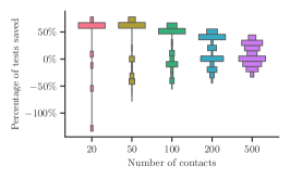
(c) Percentage of tests saved

Figure 1: Performance of our method (Algorithm  1) and Dorfman’s method for various values of the number of contacts of a diagnosed individual during their infectious period. Panel (a) shows the number of tests per contact, where the dots represent the average value and the error bars cover $90\%$ of the observations. Panel (b) shows the average pool size. Panel (c) shows the empirical distribution of the percentage of tests saved by using our method instead of Dorfman’s method, where we exclude the highest and lowest $5\%$ of observations. In all panels, we set the sensitivity and specificity to $s_{e}=s_{p}=0.95$, and sample the number of secondary infections from a truncated negative binomial distribution with mean $r=2.5$ and dispersion parameter $k=0.1$ [19, 29, 20, 30]. For each combination of method and parameter values, the averages and quantiles in all panels are estimated using $100{,}000$ samples.

We perform simulations to evaluate Algorithm 1 against Dorfman’s method in its ability to optimally trade off resources and false test outcomes in the presence of overdispersed distributions of secondary infections. To generate the infection states for each contact, we first fix a number of contacts $N$ and sample the number of secondary infections $n\sim q_{r,k,N}(n)$, where $q_{r,k,N}(n)$ is a truncated negative binomial distribution as defined in Eq. 1. Then, we select $n$ of the $N$ contacts at random and set their status to infected. To implement Dorfman’s method, we use a variation of Algorithm 1 in which the expected numbers of tests, false negatives and false positives are computed assuming an independent individual probability of infection $p=\mathbb{E}_{q_{r,k,N}}[n]/N$, using the formulas derived by Abrahamian et al. [5].

We first compare the performance of our method and Dorfman’s method at finding the pools that minimize the number of tests (i.e., $\lambda_{1}=\lambda_{2}=0$) for fixed values of the reproductive number $r$ and dispersion parameter $k$ matching estimations done during the early phase of the COVID-19 pandemic. Figure 1 summarizes the results with respect to the number of contacts $N$ of the diagnosed individuals. The results show that our method achieves a lower average number of tests across all values of $N$, with its competitive advantage being greater when the number of contacts is small and less apparent as the number of contacts is increasing. Moreover, Dorfman’ method chooses pool sizes that increase with the number of contacts while the ones chosen by our method remain relatively constant. This leads to significant differences between the distributions of the number of tests performed under the two methods. For example, as shown in Figure 1(c), when the number of contacts is $N=20$, our method is most likely to perform about $50\%$ less tests than Dorfman’s. However, due to the more conservative pool sizes given by Dorfman’s method, there is a small probability that our method ends up performing more tests, sometimes even double the amount.

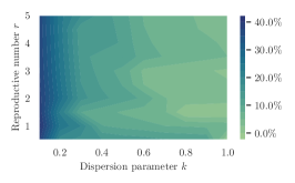
(a) $N=20$

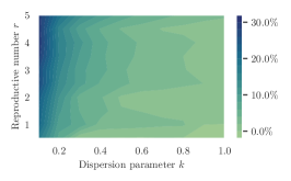
(b) $N=100$

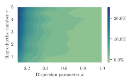
(c) $N=200$

Figure 2: Performance of our method (Algorithm 1) and Dorfman’s method for different values of the reproductive number $r$ and dispersion parameter $k$. Each panel shows the average percentage of tests saved by using our method instead of Dorfman’s method. Here, we set the sensitivity and specificity to $s_{e}=s_{p}=0.95$ and, in each experiment, we estimate the average using $100{,}000$ samples.

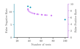
(a) $s_{e}=s_{p}=0.75$

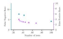
(b) $s_{e}=s_{p}=0.85$

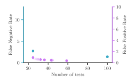
(c) $s_{e}=s_{p}=0.95$

Figure 3: Average number of tests, false negative rate and false positive rate achieved by our method (Algorithm 1) under different values of the parameters $\lambda_{1}$ and $\lambda_{2}$ and different levels of specificity $s_{e}$ and sensitivity $s_{p}$. In each panel, we either penalize the false negative rate (i.e., we vary $\lambda_{1}$ and set $\lambda_{2}=0$) or the false positive rate (i.e., we vary $\lambda_{2}$ and set $\lambda_{1}=0$). Accordingly, for the former, we show the false negative rate vs average number of tests (in blue) and, for the latter, we show the false positive rate vs average number of tests (in pink). Here, we set the number of contacts to $N=100$ and sample the number of positive infections from a truncated negative binomial distribution with mean $r=2.5$ and dispersion parameter $k=0.1$. In each experiment, we estimate averages using $100{,}000$ samples.

Next, we investigate to what extent our method offers a competitive advantage with respect to Dorfman’s method for additional values of the reproductive number $r$ and dispersion parameter $k$ different than those estimated during the early phase of the COVID-19 pandemic. Figure 2 summarizes the results, which show that our method offers the greatest competitive advantage whenever the number of secondary infections is overdispersed, i.e., $k\rightarrow 0$. Moreover, as the number of contacts $N$ increases, the competitive advantage is greater for larger values of the reproductive number $r$.

Finally, we explore the trade-off between the average number of tests that our method achieves and the false positive and negative rates, under different values of the parameters $\lambda_{1}$ and $\lambda_{2}$. Figure 3 summarizes the results, which show that, to achieve lower false negative and false positive rates, more tests need to be performed. When trading off the number of tests with the number of false positives ($\lambda_{1}=0$, $\lambda_{2}>0$), our method gradually changes the average pool size, leading to many possible trade-off points between the number of tests and the false positive rate. When $\lambda_{2}$ takes small values, the optimal solution leads to pool sizes that minimize the number of tests, while the solution consists of pools of two contacts when $\lambda_{2}$ gets significantly larger. When balancing the number of tests with the number of false negatives ($\lambda_{1}>0$, $\lambda_{2}=0$), there are only two or three possible solutions, with the extreme ones corresponding to pool sizes minimizing the number of tests and pools of size one, i.e., individual testing for all. We noticed that the expected number of false negatives in a pool grows linearly with its size for sizes greater than one, therefore, making the exact size of the pool irrelevant in terms of the expected total number of false negatives. As a consequence, this leads to only a few optimal solutions where some of the contacts are individually tested while the rest of them are split into pools.

Our results have direct implications for the allocation of limited and imperfect testing resources in future pandemics whenever there exists evidence of substantial overdispersion in the number of secondary infections. In this context, we acknowledge that more research is needed to more accurately characterize the level of overdispersion in a pandemic. Moreover, it would be interesting to extend our algorithm using distributions other that the negative binomial and practically evaluate our method in randomized control studies.

References

- [1] Sebastian Contreras et al. The challenges of containing SARS-CoV-2 via test-trace-and-isolate. Nature Communications, 12:378, January 2021.
- [2] Matthias Linden, Jonas Dehning, Sebastian B. Mohr, Jan Mohring, Michael Meyer-Hermann, Iris Pigeot, Anita Schöbel, and Viola Priesemann. The foreshadow of a second wave: An analysis of current covid-19 fatalities in germany. Deutsches Ärzteblatt Int., 2020.
- [3] Robert Dorfman. The detection of defective members of large populations. The Annals of Mathematical Statistics, 14(4):436–440, 1943.
- [4] Lois E Graff and Robert Roeloffs. Group testing in the presence of test error; an extension of the dorfman procedure. Technometrics, 14(1):113–122, 1972.
- [5] Hrayer Aprahamian, Douglas R Bish, and Ebru K Bish. Optimal risk-based group testing. Management Science, 65(9):4365–4384, 2019.
- [6] Matthew Aldridge, Oliver Johnson, and Jonathan Scarlett. Group testing: an information theory perspective. Now Foundations and Trends, 2019.
- [7] Dingzhu Du, Frank K Hwang, and Frank Hwang. Combinatorial group testing and its applications, volume 12. World Scientific, 2000.
- [8] Charles N Agoti, Martin Mutunga, Arnold W Lambisia, Domtila Kimani, Robinson Cheruiyot, Patience Kiyuka, Clement Lewa, Elijah Gicheru, Metrine Tendwa, Khadija Said Mohammed, et al. Pooled testing conserves sars-cov-2 laboratory resources and improves test turn-around time: experience on the kenyan coast. Wellcome Open Research, 5, 2020.
- [9] Jens Niklas Eberhardt, Nikolas Peter Breuckmann, and Christiane Sigrid Eberhardt. Multi-stage group testing improves efficiency of large-scale covid-19 screening. Journal of Clinical Virology, 128:104382, 2020.
- [10] Angela Felicia Sunjaya and Anthony Paulo Sunjaya. Pooled testing for expanding covid-19 mass surveillance. Disaster Medicine and Public Health Preparedness, 14(3):e42–e43, 2020.
- [11] Leon Mutesa, Pacifique Ndishimye, Yvan Butera, Jacob Souopgui, Annette Uwineza, Robert Rutayisire, Ella Larissa Ndoricimpaye, Emile Musoni, Nadine Rujeni, Thierry Nyatanyi, et al. A pooled testing strategy for identifying sars-cov-2 at low prevalence. Nature, pages 1–5, 2020.
- [12] Andreas Deckert, Till Bärnighausen, and Nicholas NA Kyei. Simulation of pooled-sample analysis strategies for covid-19 mass testing. Bulletin of the World Health Organization, 98(9):590, 2020.
- [13] Rodrigo Noriega and Matthew Samore. Increasing testing throughput and case detection with a pooled-sample bayesian approach in the context of covid-19. bioRxiv, 2020.
- [14] Roni Ben-Ami, Agnes Klochendler, Matan Seidel, Tal Sido, Ori Gurel-Gurevich, Moran Yassour, Eran Meshorer, Gil Benedek, Irit Fogel, Esther Oiknine-Djian, et al. Large-scale implementation of pooled rna extraction and rt-pcr for sars-cov-2 detection. Clinical Microbiology and Infection, 26(9):1248–1253, 2020.
- [15] Rudolf Hanel and Stefan Thurner. Boosting test-efficiency by pooled testing strategies for sars-cov-2. arXiv preprint arXiv:2003.09944, 2020.
- [16] Junan Zhu, Kristina Rivera, and Dror Baron. Noisy pooled pcr for virus testing. arXiv preprint arXiv:2004.02689, 2020.
- [17] Dillon C. Adam et al. Clustering and superspreading potential of SARS-CoV-2 infections in Hong Kong. Nature Medicine, 2020.
- [18] MSF. Too little, too late: The unacceptable neglect of the elderly in care homes during the COVID-19 epidemic in Spain, 2020.
- [19] Akira Endo et al. Estimating the overdispersion in COVID-19 transmission using outbreak sizes outside China. Wellcome Open Research, 2020.
- [20] Max SY Lau et al. Characterizing superspreading events and age-specific infectiousness of SARS-CoV-2 transmission in Georgia, USA. Proceedings of the National Academy of Sciences, 117(36), 2020.
- [21] Thomas Frieden and Christopher Lee. Identifying and interrupting superspreading events—implications for control of severe acute respiratory syndrome coronavirus 2. 2020.
- [22] Siva Athreya, Nitya Gadhiwala, and Abhiti Mishra. Effective reproduction number and dispersion under contact tracing and lockdown on COVID-19 in Karnataka. medRxiv, 2020.
- [23] Lars Lorch, Heiner Kremer, William Trouleau, Stratis Tsirtsis, Aron Szanto, Bernhard Schölkopf, and Manuel Gomez-Rodriguez. Quantifying the effects of contact tracing, testing, and containment measures in the presence of infection hotspots. arXiv preprint arXiv:2004.07641, 2020.
- [24] Myoung-don Oh et al. Middle east respiratory syndrome coronavirus superspreading event involving 81 persons, Korea 2015. Journal of Korean medical science, 30(11):1701–1705, 2015.
- [25] James O Lloyd-Smith, Sebastian J Schreiber, P Ekkehard Kopp, and Wayne M Getz. Superspreading and the effect of individual variation on disease emergence. Nature, 438(7066):355–359, 2005.
- [26] Richard A Stein. Super-spreaders in infectious diseases. International Journal of Infectious Diseases, 15(8):e510–e513, 2011.
- [27] FK Hwang. A generalized binomial group testing problem. Journal of the American Statistical Association, 70(352):923–926, 1975.
- [28] Idan Yelin, Noga Aharony, Einat Shaer Tamar, Amir Argoetti, Esther Messer, Dina Berenbaum, Einat Shafran, Areen Kuzli, Nagham Gandali, Omer Shkedi, et al. Evaluation of covid-19 rt-qpcr test in multi sample pools. Clinical Infectious Diseases, 71(16):2073–2078, 2020.
- [29] Adam J Kucharski, Petra Klepac, Andrew JK Conlan, Stephen M Kissler, Maria L Tang, Hannah Fry, Julia R Gog, W John Edmunds, Jon C Emery, Graham Medley, et al. Effectiveness of isolation, testing, contact tracing, and physical distancing on reducing transmission of sars-cov-2 in different settings: a mathematical modelling study. The Lancet Infectious Diseases, 20(10):1151–1160, 2020.
- [30] Agus Hasan, Hadi Susanto, Muhammad Firmansyah Kasim, Nuning Nuraini, Bony Lestari, Dessy Triany, and Widyastuti Widyastuti. Superspreading in early transmissions of covid-19 in indonesia. Scientific reports, 10(1):1–4, 2020.