Maximum likelihood estimation of hidden Markov models for continuous longitudinal data with missing responses and dropout

Abstract

We propose an inferential approach for maximum likelihood estimation of the hidden Markov models for continuous responses. We extend to the case of longitudinal observations the finite mixture model of multivariate Gaussian distributions with Missing At Random (MAR) outcomes, also accounting for possible dropout. The resulting hidden Markov model accounts for different types of missing pattern: ($i$) partially missing outcomes at a given time occasion; ($ii$) completely missing outcomes at a given time occasion (intermittent pattern); ($iii$) dropout before the end of the period of observation (monotone pattern). The MAR assumption is formulated to deal with the first two types of missingness, while to account for informative dropout we assume an extra absorbing state. Maximum likelihood estimation of the model parameters is based on an extended Expectation-Maximization algorithm relying on suitable recursions. The proposal is illustrated by a Monte Carlo simulation study and an application based on historical data on primary biliary cholangitis.
Keywords: Expectation-Maximization algorithm; Forward-backward recursion; Latent Markov model; Missing values; Prediction

1 Introduction

It is well known that longitudinal data (Molenberghs and Verbeke,, 2000; Diggle et al.,, 2002; Fitzmaurice et al.,, 2004; Hsiao,, 2005) are frequently affected by missing data that may arise in different ways (Little and Rubin,, 2020). The missing pattern is defined as monotone when individuals may drop out from the sample before the end of the study. In medical studies, this may be due to a terminal event, such as the death of a patient. Another type of missingness, also referred to as intermittent, is when individuals are still in the sample, but for any reason, they do not provide responses at one or more time occasions. This is the case when a clinical visit is missed. The problem is particularly severe when the missing data mechanism is informative (Little,, 1995; Albert et al.,, 2002) or not ignorable (Rubin,, 1976; Albert,, 2000; Little and Rubin,, 2020), that is, when the missingness depends on unobserved variables (Diggle and Kenward,, 1994).

The literature on statistical methods for handling missing data with repeated measurements is relatively wide. In this regards, as recently summarized in Zhou et al., (2020), we can distinguish between different approaches, which include selection models (Molenberghs et al.,, 1997; Maruotti,, 2015), pattern-mixture models (Little,, 1994; Follmann and Wu,, 1995; Kenward et al.,, 2003; Marino and Alfò,, 2020), and shared-parameter (or joint) models (Wulfsohn and Tsiatis,, 1997; Henderson et al.,, 2000; Hsieh et al.,, 2006; Rizopoulos,, 2012; Bartolucci and Farcomeni, 2015a, ; Lange et al.,, 2015; Zhang et al.,, 2020).

In this paper, we extend to the case of longitudinal observations the Finite Mixture Model (FMM) of Gaussian distributions (Titterington et al.,, 1985; McLachlan and Peel,, 2000) under the Missing At Random (MAR) assumption (Hunt and Jorgensen,, 2003; Di Zio et al.,, 2007; Eirola et al.,, 2014; Delalleau et al.,, 2018) by proposing an inferential approach to obtain exact maximum likelihood estimates of model parameters. A Hidden Markov Model (HMM; Bartolucci et al.,, 2013; Zucchini et al.,, 2016) for multivariate continuous outcomes results, which is based on conditional Gaussian distributions and can address both monotone and intermittent missing data patterns. The hidden Markov approach is of particular interest when dealing with longitudinal data (Bartolucci et al.,, 2014) as it allows us to model time dependence in a flexible way and to perform a dynamic model-based clustering (Bouveyron et al.,, 2019). The same individual may move between clusters across time, and these dynamics are provided in terms of trajectories. This is because a sequence of discrete latent variables, rather than a single latent variable, is associated with every individual, giving rise to a hidden process assumed to follow a Markov chain, generally of first-order. The states of this chain correspond to latent clusters or subpopulations of homogenous individuals.

Overall we propose an extended HMM that takes explicitly into account the following patterns of missing data: ($i$) partially missing outcomes at a given time occasion; ($ii$) completely missing outcomes at one occasion without dropout from the sample of the individual; ($iii$) dropout from the sample. The first two cases correspond to the intermittent missing responses defined above, whereas the third corresponds to a monotone missing pattern also defined as attrition. In particular, cases ($i$) and ($ii$) are dealt with under the MAR assumption, according to which the missing pattern is independent of the missing responses given the observed data. In case ($iii$) dropout is not ignorable, and specifying a model for the missing data mechanism is in order. Along with the proposal of Montanari and Pandolfi, (2018) and Spagnoli et al., (2011), we include a hidden (or latent) state, which is absorbing, in addition to the other states representing unobserved heterogeneous populations that may arise in the study.

To estimate the proposed model we rely on the maximum likelihood approach, paying particular attention to the computational aspects. In more detail, we propose an extended Expectation-Maximization (EM; Baum et al.,, 1970; Dempster et al.,, 1977; Welch,, 2003) algorithm based on suitable recursions. The estimation algorithm is also employed when there are available covariates supposed to affect the distribution of the latent process and, in particular, the initial and the transition probabilities of the Markov chain (Bartolucci et al.,, 2014). In this way, it is possible to understand the influence of the covariates on the dynamic allocation of the individuals between states over time.

In order to illustrate the proposed approach, we rely on a series of simulations that also allow us to assess the maximum likelihood estimator in terms of finite sample properties. We also show an application based on historical data about primary biliary cholangitis (or cirrhosis) collected by the Mayo Clinic from January 1974 to May 1984 (Murtaugh et al.,, 1994). Data are referred to several biochemical measurements of the liver function scheduled for the patients according to the clinical protocol over six months or one year after the first visit. Continuous and binary covariates related to the patients are also available such as age, gender, and medication use. The data are very sparse due to missing visits and the fact that some biochemical measurements were not collected at each visit. Moreover, dropout occurred due to death. The code implemented to estimate the proposed model in R (R Core Team,, 2021) is based on the package LMest (Bartolucci et al.,, 2017), and it is available on the GITHUB page at the following link (it will follow).

The remainder of the paper is organized as follows. In Section 2 we recall the FMMs of Gaussian distributions with missing data under the MAR assumption. In Section 3 we show the proposed HMM formulation. In Section 4, we outline the inferential approach proposed for estimating model parameters and aspects related to the computation of the standard errors, model selection, and decoding. In Section 5 we present the simulation study. In Section 6, we illustrate the applicative example, whereas in Section 7 we provide some conclusions. A supplementary file provides additional information on the data and results.

2 Preliminaries

In this section we outline the FMM of Gaussian distributions under the MAR assumption and with possible covariates.

2.1 Model formulation

We consider individual vectors $\mbox{\boldmath$Y$}_{i}=(Y_{1},\ldots,Y_{r})^{\prime}$ of $r$ continuous response variables, with $i=1,\ldots,n$. It is well known that the FMM of Gaussian distributions assumes that there exist $k$ components identified by the discrete latent variable $U_{i}$ such that

$$\mbox{\boldmath$Y$}_{i}|U_{i}=u\sim N(\mbox{\boldmath$\mu$}_{u},\mbox{\boldmath$\Sigma$}_{u}),\quad\quad u=1,\ldots,k.$$

In the previous expression, $\mbox{\boldmath$\mu$}_{u}$ and $\mbox{\boldmath$\Sigma$}_{u}$ denote the mean vector and the variance-covariance matrix for the same mixture component $u$, respectively. Note that the variance-covariance matrices may be assumed to be constant across the components under the assumption of homoschedasticity, which also avoids certain estimation problems (McLachlan and Peel,, 2000, Chapter 3.8). More articulated constraints on these matrices may be expressed, as proposed in Banfield and Raftery, (1993), on the basis of suitable matrix decompositions.

With missing data it is convenient to partition each response vector as $(\mbox{\boldmath$Y$}_{i}^{o},\mbox{\boldmath$Y$}_{i}^{m})^{\prime}$, where $\mbox{\boldmath$Y$}_{i}^{o}$ is the vector of observed variables and $\mbox{\boldmath$Y$}_{i}^{m}$ is that of missing variables. Using a straightforward notation, the conditional mean vectors and variance-covariance matrix may be decomposed as

$$\mbox{\boldmath$\mu$}_{u}=\begin{pmatrix}\mbox{\boldmath$\mu$}_{u}^{o}\\ \mbox{\boldmath$\mu$}_{u}^{m}\end{pmatrix},\quad\mbox{\boldmath$\Sigma$}_{u}=\begin{pmatrix}\mbox{\boldmath$\Sigma$}_{u}^{oo}&\mbox{\boldmath$\Sigma$}_{u}^{om}\\ \mbox{\boldmath$\Sigma$}_{u}^{mo}&\mbox{\boldmath$\Sigma$}_{u}^{mm}\\ \end{pmatrix},$$ (1)

where, for instance, $\mbox{\boldmath$\Sigma$}_{u}^{om}$ is the block of $\mbox{\boldmath$\Sigma$}_{u}$ containing the covariances between each observed and missing response. In this way, for the observed responses we have that

$$\mbox{\boldmath$Y$}_{i}^{o}|U_{i}=u\sim N(\mbox{\boldmath$\mu$}_{u}^{o},\mbox{\boldmath$\Sigma$}_{u}^{oo}),\quad u=1,\ldots,k.$$

Without individual covariates, each latent variable $U_{i}$ has the same distribution based on the component weights $\pi_{u}=p(U_{i}=u)$, $u=1,\ldots,k$. Consequently, the manifest distribution of the observed responses is given by

$$f(\mbox{\boldmath$y$}_{i}^{o})=\sum_{u=1}^{k}\pi_{u}\phi(\mbox{\boldmath$y$}_{i}^{o};\mbox{\boldmath$\mu$}_{u}^{o},\mbox{\boldmath$\Sigma$}_{u}^{oo}),$$ (2)

where $\mbox{\boldmath$y$}_{i}^{o}$ denotes a realization of $\mbox{\boldmath$Y$}_{i}^{o}$ and $\phi(\cdot;\cdot)$ denotes the multivariate Gaussian probability density function.

Individual covariates may be included in the model in different ways. In particular, we consider the case of component weights affected by these covariates. Let $\pi_{iu}=p(U_{i}=u|\mbox{\boldmath$x$}_{i})$ denote the class weight for component $u$ which is now specific of individual $i$ and $\mbox{\boldmath$x$}_{i}$ the vector of individual covariates, with $i=1,\ldots,n$. We assume a multinomial logit model of type

$$\log\frac{\pi_{iu}}{\pi_{i1}}=\mbox{\boldmath$x$}_{i}^{\prime}\mbox{\boldmath$\beta$}_{u},\quad u=2,\ldots,k,$$ (3)

where $\mbox{\boldmath$\beta$}_{u}$ is a vector of regression parameters. Expression (2) for the manifest distribution is obviously extended as

$$f(\mbox{\boldmath$y$}_{i}^{o})=\sum_{u=1}^{k}\pi_{iu}\phi(\mbox{\boldmath$y$}_{i}^{o};\mbox{\boldmath$\mu$}_{u}^{o},\mbox{\boldmath$\Sigma$}_{u}^{oo}).$$

2.2 Expectation-Maximization algorithm with missing data

In the presence of missing data, the observed log-likelihood can be written as

$$\ell(\mbox{\boldmath$\theta$})=\sum_{i=1}^{n}\log f(\mbox{\boldmath$y$}_{i}^{o})=\sum_{i=1}^{n}\log\left[\sum_{u=1}^{k}\pi_{u}\phi(\mbox{\boldmath$y$}_{i}^{o};\mbox{\boldmath$\mu$}_{u}^{o},\mbox{\boldmath$\Sigma$}_{u}^{oo})\right].$$

Its maximization for parameter estimation relies on the EM algorithm (Dempster et al.,, 1977). This algorithm is based on the complete-data log-likelihood that has expression

$$\ell^{*}(\mbox{\boldmath$\theta$})=\sum_{i=1}^{n}\sum_{u=1}^{k}z_{iu}\log[\pi_{u}\;\phi(\mbox{\boldmath$y$}_{i};\mbox{\boldmath$\mu$}_{u},\mbox{\boldmath$\Sigma$}_{u})],$$

where $z_{iu}$ is a binary variable indicating whether or not unit $i$ comes from component $u$.

As usual, the EM algorithm alternates two steps until convergence. The E-step consists in computing the conditional expectation of the indicator variables given the observed data and the current value of the parameters, that is,

$$\widehat{z}_{iu}=\frac{\pi_{u}\phi(\mbox{\boldmath$y$}_{i}^{o};\mbox{\boldmath$\mu$}_{u}^{o},\mbox{\boldmath$\Sigma$}_{u}^{oo})}{\sum_{v=1}^{k}\pi_{v}\phi(\mbox{\boldmath$y$}_{i}^{o};\mbox{\boldmath$\mu$}_{v}^{o},\mbox{\boldmath$\Sigma$}_{v}^{oo})}.$$ (4)

With individual covariates, this rule is modified by substituting every $\pi_{u}$ with $\pi_{iu}$.

Following the proposals in Eirola et al., (2014) and Delalleau et al., (2018), in order to account for missing data this step also includes the computation of the following conditional expectations

$${\rm E}(\mbox{\boldmath$Y$}_{i}|\mbox{\boldmath$y$}_{i}^{o},u)=\left(\begin{matrix}\mbox{\boldmath$y$}_{i}^{o}\\ {\rm E}(\mbox{\boldmath$Y$}_{i}^{m}|\mbox{\boldmath$y$}_{i}^{o},u)\end{matrix}\right),$$ (5)

where

$${\rm E}(\mbox{\boldmath$Y$}_{i}^{m}|\mbox{\boldmath$y$}_{i}^{o},u)=\mbox{\boldmath$\mu$}_{u}^{m}+\mbox{\boldmath$\Sigma$}_{u}^{mo}(\mbox{\boldmath$\Sigma$}_{u}^{oo})^{-1}(\mbox{\boldmath$y$}_{i}^{o}-\mbox{\boldmath$\mu$}_{u}^{o}),$$

and of the conditional variances

$$\begin{split}\mathrm{Var}(\mbox{\boldmath$Y$}_{i}|\mbox{\boldmath$y$}_{i}^{o},u)=\left(\begin{matrix}\mbox{\boldmath$O$}&\mbox{\boldmath$O$}\\ \mbox{\boldmath$O$}&\mbox{\boldmath$\Sigma$}_{u}^{mm}-\mbox{\boldmath$\Sigma$}_{u}^{mo}(\mbox{\boldmath$\Sigma$}_{u}^{oo})^{-1}\mbox{\boldmath$\Sigma$}_{u}^{om}\end{matrix}\right),\end{split}$$

where $O$ is a matrix of zeros of suitable dimension. The above expressions originate from the fact that the missing values’ conditional distribution also follows a multivariate Gaussian distribution (Anderson,, 2003).

The M-step consists in updating the model parameters by maximizing the expected value of $\ell^{*}(\mbox{\boldmath$\theta$})$ obtained at the E-step. This maximization leads to the following updating rules for the mean vector and the variance-covariance matrices:

$$\mbox{\boldmath$\mu$}_{u} = \frac{1}{\sum_{i=1}^{n}\widehat{z}_{iu}}\sum_{i=1}^{n}\widehat{z}_{iu}{\rm E}(\mbox{\boldmath$Y$}_{i}|\mbox{\boldmath$y$}_{i}^{o},u),$$ (6)

$$\mbox{\boldmath$\Sigma$}_{u} = \frac{1}{\sum_{i=1}^{n}\widehat{z}_{iu}}\sum_{i=1}^{n}\widehat{z}_{iu}\bigg{\{}\mathrm{Var}(\mbox{\boldmath$Y$}_{i}|\mbox{\boldmath$y$}_{it}^{o},u)+[{\rm E}(\mbox{\boldmath$Y$}_{i}|\mbox{\boldmath$y$}_{i}^{o},u)-\mbox{\boldmath$\mu$}_{u}][{\rm E}(\mbox{\boldmath$Y$}_{i}|\mbox{\boldmath$y$}_{i}^{o},u)-\mbox{\boldmath$\mu$}_{u}]^{\prime}\bigg{\}}.$$ (7)

The rule in (7) is suitably modified by summing the numerator for all $u$, and dividing the sum by $n$, under the constraint of homoschedasticity. The component weights are updated as

$$\pi_{u}=\frac{\sum_{i=1}^{n}\widehat{z}_{iu}}{n},\quad\quad\quad u=1,\ldots,k,$$

whereas with individual covariates we maximize the complete log-likelihood component

$$\sum_{i=1}^{n}\sum_{u=1}^{k}\widehat{z}_{iu}\log\pi_{iu}$$

with respect to the parameter vectors $\mbox{\boldmath$\beta$}_{2},\ldots,\mbox{\boldmath$\beta$}_{k}$ defined in Expression (3) by a Newton-Raphson algorithm.

These two steps are repeated until convergence, which is checked on the basis of the relative log-likelihood difference, that is,

$$\frac{\mid\ell(\mbox{\boldmath$\theta$}^{(s)})-\ell(\mbox{\boldmath$\theta$}^{(s-1)})\mid}{\mid\ell(\mbox{\boldmath$\theta$}^{(s)})\mid}\leq\epsilon,$$

where $\mbox{\boldmath$\theta$}^{(s)}$ is the vector of parameter estimates obtained at the end of the $s$th M-step and $\epsilon$ is a suitable tolerance level (e.g., 10^-8). A crucial aspect is that of initialization of the algorithm to deal with the likelihood multimodality. In this regard, it is important to rely on different strategies, even based on random rules for choosing the model parameters’ starting values.

2.3 Model selection and clustering

Selection of the number of components is an important aspect in applying FMMs (McLachlan and Peel,, 2000, Chapter 6). Typically, this choice is based on information criteria such as the Akaike Information Criterion (AIC; Akaike,, 1973) or the Bayesian Information Criterion (BIC; Schwarz,, 1978), obtained through penalizations of the maximum log-likelihood. In particular, the AIC index is expressed as

$$AIC_{k}=-2\widehat{\ell}_{k}+2\#par,$$

whereas the BIC index has expression

$$BIC_{k}=-2\widehat{\ell}_{k}+\log(n)\#par,$$

where $\widehat{\ell}_{k}$ denotes the maximum of the log-likelihood of the FMM with $k$ components and $\#par$ denotes the number of free parameters. To select the optimal number of components, we estimate a series of models for increasing values of $k$, and we select the one corresponding to the minimum value of these indexes. The BIC is usually preferred to the AIC as the latter tends to overestimate the number of components (McLachlan and Peel,, 2000, Chapter 6.9).

Finally, on the basis of the estimation results, model-based clustering is performed with the Maximum-A-Posteriori (MAP) rule, consisting of assigning unit $i$ to the latent component corresponding to the maximum over $u$ of the posterior probability computed as in (4). The selected component for unit $i$ is dented by $\widehat{u}_{i}$. Note that, with missing data, we also perform a sort of multiple imputation that allows us to predict the missing responses conditionally or unconditionally to the model component. In the first case the predicted value is simply $\widehat{\mbox{\boldmath$y$}}_{i}={\rm E}(\mbox{\boldmath$Y$}_{i}|\mbox{\boldmath$y$}_{i}^{o},\widehat{u}_{i})$, while for the unconditional case it is computed as

$$\widetilde{\mbox{\boldmath$y$}}_{i}=\sum_{u=1}^{k}\widehat{z}_{iu}{\rm E}(\mbox{\boldmath$Y$}_{i}|\mbox{\boldmath$y$}_{i}^{o},u),$$

where the expected value is defined in (5).

3 Proposed hidden Markov model with missing data

Considering the FMM outlined in the previous section, in the following we propose an HMM to deal with intermittent and monotone missing observations.

3.1 Model formulation

We denote by $\mbox{\boldmath$Y$}_{it}=(Y_{i1t},\ldots,Y_{irt})^{\prime}$ the vector of $r$ continuous response variables measured at time $t$, with $t=1,\ldots,T_{i}$. Note that the number of time occasions $T_{i}$ is specific for each individual $i$, with $i=1,\ldots,n$. In this way, we also conceive unbalanced panels that, for example, are due to a different number of scheduled visits for every individual in a medical study. As already mentioned, in a longitudinal extension it is also important to account for dropout that gives rise to monotone informative missing data. In this regard, we first introduce the indicator variable $D_{it}$ for the dropout, which assumes a value equal to 0 if unit $i$ is still in the panel at occasion $t$ and equal to 1 if the same unit has dropped out. It is worth noting that the event of dropout at time $t$, so that $D_{it}=1$, implies that $D_{i,t+1},\ldots,D_{iT_{i}}=1$. Obviously, even if $D_{it}=0$, we may still have a missing observation at occasion $t$ due to the intermittent missing data pattern with all or some of the outcomes that are not observed.

The general HMM formulation assumes the existence of a latent process for each individual $i$, denoted by $\mbox{\boldmath$U$}_{i}=(U_{i1},\ldots,U_{iT_{i}})^{\prime}$, which affects the distribution of the response variables and is assumed to follow a first-order Markov chain with a certain number of states equal to $k+1$. This model may account for dropout by adding an extra latent state, the $(k+1)$-th, defined as an absorbing state, in the sense that once it has been reached, then it is not possible to move away from it. This proposal has been previously introduced in Montanari and Pandolfi, (2018).

The HMM has two components: the measurement (sub)-model, concerning the conditional distribution of the response variables given the latent process, and the latent (sub)-model, concerning the distribution of the latent process. Regarding the first component, we assume that the response vectors are conditionally independent given the hidden state and that, as in the FMM presented in Section 2, for the first $k$ states, the response vectors have Gaussian distribution with specific mean vector and variance-covariance matrix. More precisely, we assume that

$$\mbox{\boldmath$Y$}_{it}|U_{it}=u,D_{it}=0\sim N(\mbox{\boldmath$\mu$}_{u},\mbox{\boldmath$\Sigma$}),\quad\quad u=1,\ldots,k,$$

where the means $\mbox{\boldmath$\mu$}_{u}$, $u=1,\ldots,k$, are specific of each state, and the variance-covariance matrix $\Sigma$ is assumed to be constant across states under the assumption of homoschedasticity. Reducing the model complexity drives this choice, but homoschedasticity can be suitably relaxed if necessary. In addition, we assume that

$$P(D_{it}=d|U_{it}=u)=\left\{\begin{array}[]{ll}1&\text{with $d=0$ and $u=1,\ldots,k$ }\\ \vspace{2mm}&\>\>\text{\rm or $d=1$ and $u=k+1$},\\ 0&\text{otherwise}.\end{array}\right.$$

In order to account for intermittent missing responses, we consider the partition ${\mbox{\boldmath$Y$}}_{it}=(\mbox{\boldmath$Y$}_{it}^{o},\mbox{\boldmath$Y$}_{it}^{m})^{\prime}$, where $\mbox{\boldmath$Y$}_{it}^{o}$ is the vector of the observed responses and $\mbox{\boldmath$Y$}_{it}^{m}$ is referred to the missing data. As for the model illustrated in Section 2, we consider a decomposition of the conditional mean vector and the variance-covariance matrix; see Expression (1). Consequently, we have that

$$\mbox{\boldmath$Y$}_{it}^{o}|U_{it}=u,D_{it}=0\sim N(\mbox{\boldmath$\mu$}_{u}^{o},\mbox{\boldmath$\Sigma$}^{oo}),\quad\quad u=1,\ldots,k.$$

Note that the distribution of $\mbox{\boldmath$Y$}_{it}^{o}$ given $U_{it}=k+1$ and $D_{it}=1$ does not need to be defined.

Finally, the parameters of the latent model are the initial probabilities

$$\pi_{u}=p(U_{i1}=u),\quad\quad u=1,\ldots k,$$

and the transition probabilities

$$\pi_{u|\overline{u}}=p(U_{it}=u|U_{i,t-1}=\overline{u}),\quad\quad t=2,\ldots,T_{i},\;\>\ \overline{u},u=1,\ldots,k,$$

where $u$ denotes a realization of $U_{it}$ and $\overline{u}$ a realization of $U_{i,t-1}$. Note that the transition probabilities are assumed to be time homogeneous to reduce the number of free parameters, but even this assumption may be relaxed at the occurrence. Moreover, given the interpretation of the latent state referred to as dropout, the transition probabilities are suitably constrained as

$$\pi_{k+1|k+1}=1,\quad\pi_{u|k+1}=0,\quad\quad u=1,\ldots,k.$$

Therefore, once a subject reaches the $(k+1)$-th latent state, he/she yields missing values until the end of the study. The interest in modeling this extra state is evident when the model includes individual covariates, as shown in the following.

In the present formulation, the manifest distribution is expressed with reference to the observed data represented by $\mathcal{Y}_{i}^{o}=\{\mbox{\boldmath$y$}_{it}^{o},t=1,\ldots,T_{i}:d_{it}=0\}$, which is the set of vectors $\mbox{\boldmath$y$}_{it}^{o}$ observed when $d_{it}=0$, for $i=1,\ldots,n$. Denoting by $\mbox{\boldmath$d$}_{i}$ the vector of the observed indicator variables $D_{it}$ for individual $i$, we have that

$$f(\mbox{\boldmath$d$}_{i},\mathcal{Y}_{i}^{o}) = \sum_{\mbox{\scriptsize\boldmath{$u$}}_{i}}f(\mathcal{Y}_{i}^{o}|\mbox{\boldmath$D$}_{i}=\mbox{\boldmath$d$}_{i},\mbox{\boldmath$U$}_{i}=\mbox{\boldmath$u$}_{i})P(\mbox{\boldmath$D$}_{i}=\mbox{\boldmath$d$}_{i}|\mbox{\boldmath$U$}_{i}=\mbox{\boldmath$u$}_{i})P(\mbox{\boldmath$U$}_{i}=\mbox{\boldmath$u$}_{i})$$ (8)

$$= \sum_{\mbox{\scriptsize\boldmath{$u$}}_{i}}\left[\prod_{t=1}^{T_{i}}f(\mbox{\boldmath$y$}_{it}^{o}|d_{it},u_{it})\>p(d_{it}|u_{it})\right]\left(\pi_{u_{i1}}\prod_{t=2}^{T_{i}}\pi_{u_{it}|u_{i,t-1}}\right).$$

As usual in dealing with HMMs, to efficiently compute this distribution, we can rely on a forward recursion (Baum et al.,, 1970; Welch,, 2003).

The above formulation allows us to characterize the process generating informative dropout and to study the probability of transition from the estimated latent states to the dropout state. More in detail, starting from the EM algorithm illustrated in Section 2.2, we develop an inferential approach to obtain exact maximum likelihood estimates of model parameters under the MAR assumption for the intermittent missingness and with informative dropout. The resulting EM algorithm also includes suitable forward-backward recursions to perform the E-step (Baum et al.,, 1970; Welch,, 2003).

3.2 Inclusion of individual covariates

Longitudinal data allow for a precise assessment of the effect of individual covariates and this aspect is particularly relevant when these variables are related to a certain treatment as in the empirical illustration provided in Section 6. In the HMM formulation, individual covariates may be included in the measurement model or in the latent model; for a general review see Bartolucci et al., (2013) and (Bartolucci et al.,, 2014). In the first case, the conditional distribution of the response variables given the latent states must be suitably parameterized. In such a situation, the latent variables account for the unobserved heterogeneity that is allowed to be time-varying (Bartolucci and Farcomeni,, 2009). When covariates are included in the latent model, the interest is in modeling the effect of covariates on the distribution of the latent process (Vermunt et al.,, 1999). This formulation is relevant when the response variables measure an individual characteristic of interest represented by the latent variables.

In this work, we consider the second formulation and we adopt a multinomial parameterization for the initial and transition Markov chain probabilities. More in detail, let $\mbox{\boldmath$x$}_{it}$ denote the vector of individual covariates available at the $t$-th time occasion for individual $i$. Now the initial and transition probabilities are individual specific and denoted by $\pi_{iu}=p(U_{i1}=u|\mbox{\boldmath$x$}_{i1})$, $u=1,\ldots,k$, and $\pi_{i,u|\overline{u}}=p(U_{it}=u|U_{i,t-1}=\overline{u},\mbox{\boldmath$x$}_{it})$, $t=2,\ldots,T$, $\overline{u},u=1,\ldots,k$, respectively. We rely on the following parameterization

$$\log\frac{\pi_{iu}}{\pi_{i1}}=\beta_{0u}+\mbox{\boldmath$x$}_{i1}^{\prime}\mbox{\boldmath$\beta$}_{1u},\quad u=2,\ldots,k,$$ (9)

for the initial probabilities and on the following parametrization

$$\log\frac{\pi_{i,u|\overline{u}}}{\pi_{i,\overline{u}|\overline{u}}}=\gamma_{0\overline{u}u}+\mbox{\boldmath$x$}_{it}^{\prime}\mbox{\boldmath$\gamma$}_{1\overline{u}u},\quad\overline{u}=1,\ldots,k,\;\>\ u=1,\ldots,k+1,\;\>\ \overline{u}\neq u,$$ (10)

for the transition probabilities. In the above expressions, $\mbox{\boldmath$\beta$}_{u}=(\beta_{0u},\mbox{\boldmath$\beta$}_{1u}^{\prime})^{\prime}$ and $\mbox{\boldmath$\gamma$}_{\overline{u}u}=(\gamma_{0\overline{u}u},\mbox{\boldmath$\gamma$}_{1\overline{u}u}^{\prime})^{\prime}$ are parameter vectors to be estimated which are collected in the matrices $B$ and $\Gamma$, respectively. Note that parameters in $B$ are not affected by the presence of the extra state since no unit is in the dropout state at the beginning of the study. On the other hand, parameters in $\Gamma$ are properly constrained to avoid transitions from the latent absorbing state.

Finally, expression (8) for the manifest distribution is extended as

$$f(\mbox{\boldmath$d$}_{i},\mathcal{Y}_{i}^{o})=\sum_{\mbox{\scriptsize\boldmath{$u$}}_{i}}\left[\prod_{t=1}^{T_{i}}f(\mbox{\boldmath$y$}_{it}^{o}|d_{it},u_{it})\>p(d_{it}|u_{it})\right]\left(\pi_{i,u_{i1}}\prod_{t=2}^{T_{i}}\pi_{i,u_{it}|u_{i,t-1}}\right).$$ (11)

4 Model inference

In the following, we first illustrate the proposed inferential approach based on the maximization of the log-likelihood function. Then, we outline the strategy for the initialization of the estimation algorithm. Finally, we discuss issues related to the computation of the standard errors, selection of the number of states, and model-based dynamic clustering.

4.1 Maximum log-likelihood estimation with missing responses

Assuming independence between sample units, the log-likelihood referred to the observed data is

$$\ell(\mbox{\boldmath$\theta$})=\sum_{i=1}^{n}\log f(\mbox{\boldmath$d$}_{i},\mathcal{Y}_{i}^{o}).$$

In the above expression, $\theta$ is the vector of all model parameters and $f(\mbox{\boldmath$d$}_{i},\mathcal{Y}_{i}^{o})$ is the manifest distribution of the observed responses defined in (8) and in (11) with covariates. In order to estimate the parameters, we maximize $\ell(\mbox{\boldmath$\theta$})$ by an EM algorithm based on a complete-data log-likelihood that may be expressed as the sum of three components that are maximized separately:

$$\begin{split}\ell^{*}(\mbox{\boldmath$\theta$})=\ell_{1}^{*}(\mbox{\boldmath$\theta$})+\ell_{2}^{*}(\mbox{\boldmath$\theta$})+\ell_{3}^{*}(\mbox{\boldmath$\theta$}),\end{split}$$

where

$$\ell_{1}^{*}(\mbox{\boldmath$\theta$}) = \sum_{i=1}^{n}\sum_{\begin{subarray}{c}t=1\\ (d_{it}=0)\end{subarray}}^{T_{i}}\sum_{u=1}^{k}z_{itu}\log f(\mbox{\boldmath$y$}_{it}|D_{it}=0,u),$$

$$\ell_{2}^{*}(\mbox{\boldmath$\theta$}) = \sum_{i=1}^{n}\sum_{u=1}^{k}z_{i1u}\log\pi_{u},$$

$$\ell_{3}^{*}(\mbox{\boldmath$\theta$}) = \sum_{i=1}^{n}\sum_{t=2}^{T_{i}}\sum_{\overline{u}=1}^{k+1}\sum_{u=1}^{k+1}z_{it\overline{u}u}\log\pi_{u|\overline{u}}.$$

In the above expressions, $z_{itu}=I(u_{it}=u)$ is an indicator variable equal to 1 if individual $i$ is in latent state $u$ at time $t$ and $z_{it\overline{u}u}=z_{i,t-1,\overline{u}}\;z_{itu}$ is the indicator variable for the transition from state $\overline{u}$ to state $u$ of individual $i$ at time occasion $t$. When individual covariates are available, expressions for $\ell_{2}^{*}(\mbox{\boldmath$\theta$})$ and $\ell_{3}^{*}(\mbox{\boldmath$\theta$})$ are modified by substituting every $\pi_{u}$ and $\pi_{u|\overline{u}}$ with $\pi_{iu}$ and $\pi_{i,u|\overline{u}}$, respectively, which in turn are formulated as in expressions (9) and (10). Also note that in $\ell_{1}^{*}(\mbox{\boldmath$\theta$})$, the sum over $t$ is computed only when $d_{it}=0$, whereas in $\ell_{3}^{*}(\mbox{\boldmath$\theta$})$ the last two sums also involve the absorbing hidden state, $k+1$. More explicitly, the first component of the complete log-likelihood function may be written as

$$\begin{split}\log f(\mbox{\boldmath$y$}_{it}|D_{it}=0,u)=-\frac{1}{2}\log(|\mbox{\boldmath$\Sigma$}|)-\frac{1}{2}(\mbox{\boldmath$y$}_{it}-\mbox{\boldmath$\mu$}_{u})^{\prime}\mbox{\boldmath$\Sigma$}^{-1}(\mbox{\boldmath$y$}_{it}-\mbox{\boldmath$\mu$}_{u}).\end{split}$$

Therefore, we have that

$$\ell_{1}^{*}(\mbox{\boldmath$\theta$})=\sum_{i=1}^{n}\bigg{\{}-\frac{T_{i}-d_{i+}}{2}\log(|\mbox{\boldmath$\Sigma$}|)-\frac{1}{2}\sum_{\begin{subarray}{c}t=1\\ (d_{it}=0)\end{subarray}}^{T_{i}}\sum_{u=1}^{k}z_{itu}{\rm tr}\left[\mbox{\boldmath$\Sigma$}^{-1}(\mbox{\boldmath$y$}_{it}-\mbox{\boldmath$\mu$}_{u})(\mbox{\boldmath$y$}_{it}-\mbox{\boldmath$\mu$}_{u})^{\prime}\right]\bigg{\}},$$

where $d_{i+}=\sum_{t=1}^{T_{i}}d_{it}$.

At the E-step of the EM algorithm we compute the posterior expected value of the indicator variables given the observed data and the current value of the parameters. In particular, these expected values correspond to the following quantities

$$\widehat{z}_{itu} = p(U_{it}=u|\mbox{\boldmath$y$}_{it},\mbox{\boldmath$d$}_{i}),\quad t=1,\ldots,T_{i},\;u=1,\ldots,k+1$$ (12)

$$\widehat{z}_{it\overline{u}u} = p(U_{it}=u,U_{i,t-1}=\overline{u}|\mbox{\boldmath$y$}_{it},\mbox{\boldmath$d$}_{i}),\quad t=2,\ldots,T_{i},\;\>\ \overline{u},u=1,\ldots,k+1,$$ (13)

computed by means of forward-backward recursions of Baum et al., (1970) and Welch, (2003); for an illustration see Bartolucci et al., (2013). We stress that when $d_{it}=1$, that is, when unit $i$ has dropped out at occasion $t$, we have $\widehat{z}_{isu}=0$, for $u=1,\ldots,k$ and $s=t,\ldots,T_{i}$, and $\widehat{z}_{is,k+1}=1$ for $s=t,\ldots,T_{i}$. With individual covariates, the posterior probabilities in (12) and (13) are expressed by $\widehat{z}_{itu}=p(U_{it}=u|\mbox{\boldmath$y$}_{it},\mbox{\boldmath$d$}_{i},\mbox{\boldmath$x$}_{it})$ and $\widehat{z}_{it\overline{u}u}=p(U_{it}=u,U_{i,t-1}=\overline{u}|\mbox{\boldmath$y$}_{it},\mbox{\boldmath$d$}_{i},\mbox{\boldmath$x$}_{it})$, respectively. Furthermore, when $d_{it}=0$, the E-step also includes the computation of the following expected values resulting from the MAR assumption for the missing observations

$$\begin{split}{\rm E}(\mbox{\boldmath$Y$}_{it}|\mbox{\boldmath$y$}_{it}^{o},u)=\left(\begin{matrix}\mbox{\boldmath$y$}_{it}^{o}\\ \mbox{\boldmath$\mu$}_{u}^{m}+\mbox{\boldmath$\Sigma$}^{mo}(\mbox{\boldmath$\Sigma$}^{oo})^{-1}(\mbox{\boldmath$y$}_{it}^{o}-\mbox{\boldmath$\mu$}_{u}^{o})\end{matrix}\right),\end{split}$$ (14)

$${\rm E}\left[(\mbox{\boldmath$Y$}_{it}-\mbox{\boldmath$\mu$}_{u})(\mbox{\boldmath$Y$}_{it}-\mbox{\boldmath$\mu$}_{u})^{\prime}|\mbox{\boldmath$y$}_{it}^{o},u\right] = \mathrm{Var}(\mbox{\boldmath$Y$}_{it}|\mbox{\boldmath$y$}_{it}^{o})+{\rm E}(\mbox{\boldmath$Y$}_{it}|\mbox{\boldmath$y$}_{it}^{o},u){\rm E}(\mbox{\boldmath$Y$}_{it}|\mbox{\boldmath$y$}_{it}^{o},u)^{\prime}$$

$$-\mbox{\boldmath$\mu$}_{u}{\rm E}(\mbox{\boldmath$Y$}_{it}|\mbox{\boldmath$y$}_{it}^{o},u)^{\prime}-{\rm E}(\mbox{\boldmath$Y$}_{it}|\mbox{\boldmath$y$}_{it}^{o},u)\mbox{\boldmath$\mu$}_{u}^{\prime}+\mbox{\boldmath$\mu$}_{u}\mbox{\boldmath$\mu$}_{u}^{\prime}=$$

$$= \mathrm{Var}(\mbox{\boldmath$Y$}_{it}|\mbox{\boldmath$y$}_{it}^{o})+[E(\mbox{\boldmath$Y$}_{it}|\mbox{\boldmath$y$}_{it}^{o},u)-\mbox{\boldmath$\mu$}_{u}][E(\mbox{\boldmath$Y$}_{it}|\mbox{\boldmath$y$}_{it}^{o},u)-\mbox{\boldmath$\mu$}_{u}]^{\prime},$$

where

$$\begin{split}\mathrm{Var}(\mbox{\boldmath$Y$}_{it}|\mbox{\boldmath$y$}_{it}^{o})=\left(\begin{matrix}\mbox{\boldmath$O$}&\mbox{\boldmath$O$}\\ \mbox{\boldmath$O$}&\mbox{\boldmath$\Sigma$}^{mm}-\mbox{\boldmath$\Sigma$}^{mo}(\mbox{\boldmath$\Sigma$}^{oo})^{-1}\mbox{\boldmath$\Sigma$}^{om}\end{matrix}\right).\end{split}$$

At the M-step of the EM algorithm, we update the model parameters by considering the closed form solution for the means

$$\mbox{\boldmath$\mu$}_{u}=\frac{1}{\sum_{i=1}^{n}\sum_{\begin{subarray}{c}t=1\\ (d_{it}=0)\end{subarray}}^{T_{i}}\widehat{z}_{itu}}\sum_{i=1}^{n}\sum_{\begin{subarray}{c}t=1\\ (d_{it}=0)\end{subarray}}^{T_{i}}\widehat{z}_{itu}{\rm E}(\mbox{\boldmath$Y$}_{it}|\mbox{\boldmath$y$}_{it}^{o},u),\quad u=1,\ldots,k,$$

and we update $\Sigma$ as

$$\Sigma = \frac{1}{\sum_{i=1}^{n}(T_{i}-d_{i+})}\sum_{i=1}^{n}\sum_{\begin{subarray}{c}t=1\\ (d_{it}=0)\end{subarray}}^{T_{i}}\sum_{u=1}^{k}\widehat{z}_{itu}\bigg{\{}\mathrm{Var}(\mbox{\boldmath$Y$}_{it}|\mbox{\boldmath$y$}_{it}^{o})+[{\rm E}(\mbox{\boldmath$Y$}_{it}|\mbox{\boldmath$y$}_{it}^{o},u)-\mbox{\boldmath$\mu$}_{u}][{\rm E}(\mbox{\boldmath$Y$}_{it}|\mbox{\boldmath$y$}_{it}^{o},u)-\mbox{\boldmath$\mu$}_{u}]^{\prime}\bigg{\}}$$

that directly compare with Expressions (6) and (7).

Finally, without individual covariates the initial and transition probabilities may be updated as

$$\pi_{u} = \frac{\sum_{i=1}^{n}\widehat{z}_{i1u}}{n},\quad u=1,\ldots,k,$$

$$\pi_{u|\overline{u}} = \frac{\sum_{i=1}^{n}\sum_{t=2}^{T_{i}}\widehat{z}_{it\overline{u}u}}{\sum_{i=1}^{n}\sum_{t=2}^{T_{i}}\widehat{z}_{i,t-1,u}},\quad\overline{u},u=1,\ldots,k+1,$$

whereas, with individual covariates, in order to update the latent model parameters we maximize the complete log-likelihood components $\ell_{2}^{*}(\mbox{\boldmath$\theta$})$ and $\ell_{3}^{*}(\mbox{\boldmath$\theta$})$, with respect to $B$ and $\Gamma$, by a Newton-Raphson algorithm.

4.2 Algorithm initialization

As already mentioned for FMMs, the initialization of the EM algorithm plays a central role as the model log-likelihood is typically multimodal. This is a common problem in the estimation of discrete latent variable models implying that the EM algorithm may converge to one of the local modes that does not correspond to the global maximum. In such a situation, a multi-start strategy, based both on a deterministic and a random starting rule, is necessary. More in detail, the deterministic rule consists in computing the starting values of the parameters of the measurement model, $\mbox{\boldmath$\mu$}_{u}$, $u=1,\ldots,k$, and $\Sigma$, on the basis of descriptive statistics (mean and covariance matrix) of the observed outcomes. The starting values for the initial probabilities $\pi_{u}$ are chosen as $1/k$, for $u=1,\ldots,k$, also including the constraint $\pi_{k+1}=0$. For the transition probabilities we use $\pi_{u|\overline{u}}=(h+1)/[h+(k+1)]$ when $u=\overline{u}$ and $\pi_{u|\overline{u}}=1/[h+(k+1)]$ when $u\neq\overline{u}$, for $u=1,\ldots,k+1$ and $\overline{u}=1,\ldots,k$, where $h$ is a suitable constant; for instance, in the application illustrated in Section 6 we use $h=9$. We also constrain the last row of the transition matrix to be $\pi_{u|k+1}=0$ for $u=1,\ldots,k$ and $\pi_{k+1|k+1}=1$. The random starting rule is based on values generated from a Gaussian distribution for the vectors $\mbox{\boldmath$\mu$}_{u}$, $u=1,\ldots,k$, and on suitable normalized random numbers drawn from a uniform distribution between 0 and 1 for both initial and transition probabilities. The starting values for the variance-covariance matrix are again chosen according to the covariance of the observed outcomes. The same rules may be suitably adapted when individual covariates are included in the model; in this case, the initialization of the EM algorithm directly refers to parameters in $B$ and $\Gamma$.

Overall, for a given $k$, the inference is based on the solution corresponding to the largest value of the log-likelihood at convergence, which typically corresponds to the global maximum. The estimates obtained in this way are denoted by $\widehat{\mbox{\boldmath$\theta$}}$.

4.3 Standard errors, model selection and clustering

Once parameter estimates are computed for a given number of latent states $k$, and collected in $\widehat{\mbox{\boldmath$\theta$}}$, the corresponding standard errors may be obtained on the basis of different methods. In this work, due to its ease of implementation and robustness of the corresponding results, we mainly rely on a non-parametric bootstrap procedure (Davison and Hinkley,, 1997). This is performed by repeatedly sampling with replacement the data from the original sample, and fitting the proposed HMM with the selected number of states on these bootstrap samples. A drawback of this method is the high computational cost due to the need to fit the HMM for each resampled dataset. A possible approach to reduce the computational burden is to select as starting values of the proposed EM algorithm the parameters obtained for the observed data.

An alternative method to obtain standard errors is on the basis of the observed information matrix $J(\widehat{\mbox{\boldmath$\theta$}})$. We compute this matrix through numerical methods as proposed in Bartolucci and Farcomeni, (2009), that is, as minus the numerical derivative of the score vector at convergence. The score vector, in turn, is obtained as the first derivative of the expected value of the complete data log-likelihood, which is based on the expected frequencies $\widehat{z}_{itu}$ and $\widehat{z}_{it\overline{u}u}$ corresponding to $\widehat{\mbox{\boldmath$\theta$}}$ (Oakes,, 1999). Accordingly, standard errors for the parameter estimates are obtained as the square root of the diagonal elements of the inverse of the observed information matrix $J(\widehat{\mbox{\boldmath$\theta$}})^{-1}$; see also Bartolucci and Farcomeni, 2015b .

Concerning model selection, we rely on information criteria common to the finite-mixture literature (McLachlan and Peel,, 2000) and, in particular, on the BIC, which outperforms the alternative information criteria as examined in Bacci et al., (2014). Based on this selection approach, we estimate a series of models for increasing values of $k$, and we select the number of latent states corresponding to the minimum value of the BIC index. However, as typically happens in applications to complex and high dimensional data, the BIC index may continue to decrease for each additional state added until a very large value of $k$. In such a situation, it is advisable to choose the value of $k$ that represents a suitable compromise between goodness-of-fit and interpretability of the resulting latent states as implemented, among others, in Montanari and Pandolfi, (2018). It is also useful to visually display the values of the index against increasing $k$ so as to look for the “elbow”, that is, a change of slope in the curve suggesting the optimal number of states (Nylund-Gibson and Choi,, 2018).

Finally, once the number of states is selected, dynamic clustering is performed by assigning each unit to a latent state at each time occasion. The EM algorithm directly provides the estimated posterior probabilities of $U_{it}$, as defined in (12). These probabilities can be directly used to perform local decoding so as to predict the latent states of each unit $i$ at each time occasion $t$. To obtain the prediction of the latent trajectories of a unit across time, that is, the most a posteriori likely sequence of hidden states, we also employ the so-called global decoding, which is based on an adaptation of the Viterbi algorithm (Viterbi,, 1967); see also Juang and Rabiner, (1991).

Even in this case, it is possible to perform multiple imputation of the missing responses conditionally or unconditionally to the predicted latent state. As in the context of FMMs, in the conditional case the predicted value is simply $\widehat{\mbox{\boldmath$y$}}_{it}={\rm E}(\mbox{\boldmath$Y$}_{it}|\mbox{\boldmath$y$}_{it}^{o},\widehat{u}_{it})$, where $\widehat{u}_{it}$ are the predicted states. The unconditional prediction of the missing responses is instead computed as

$$\widetilde{\mbox{\boldmath$y$}}_{it}=\sum_{u=1}^{k}\widehat{z}_{itu}{\rm E}(\mbox{\boldmath$Y$}_{it}|\mbox{\boldmath$y$}_{it}^{o},u),$$

where the expected value is defined as in (14).

The functions used to perform maximum likelihood estimation of the proposed HMM with missing values, to compute standard errors, and to perform non-parametric bootstrap, are implemented by extending the functions of the R package LMest (Bartolucci et al.,, 2017) and are available at the GITHUB page (GitHub link with the code will follow).

5 Simulation Study

In the following, we illustrate the simulation design carried out to assess the performance of the proposed approach. It is developed varying the sample size, the number of hidden states, and the assumed proportion of intermittent missing responses and informative dropout observations. Here, we also aim at evaluating whether the proposed inferential approach allows us to identify the correct data generating process in terms of model parameters’ recovery.

5.1 Simulation design

We randomly drew $B=250$ samples of size $n=500,1000$ from an HMM with a number of hidden states equal to $k=2,3$. We also considered a number of time occasions $T=5$ and $r=3$ continuous response variables, and a varying proportion of intermittent missing responses, that is, $p_{\rm miss}=0.01,0.05,0.10,0.25$.

Regarding the measurement model, we considered the following values for the conditional means:

$$k=2:\mbox{\boldmath$\mu$}_{1}=\begin{pmatrix}[r]-2\\ -2\\ 0\end{pmatrix},\;\mbox{\boldmath$\mu$}_{2}=\begin{pmatrix}[r]0\\ 2\\ 2\end{pmatrix},$$

$$k=3:\mbox{\boldmath$\mu$}_{1}=\begin{pmatrix}[r]-2\\ -2\\ 0\end{pmatrix},\;\mbox{\boldmath$\mu$}_{2}=\begin{pmatrix}[r]0\\ 0\\ 0\end{pmatrix},\;\mbox{\boldmath$\mu$}_{3}=\begin{pmatrix}[r]0\\ 2\\ 2\end{pmatrix},$$

and the following variance-covariance matrix assumed constant across states:

$$\mbox{\boldmath$\Sigma$}=\begin{pmatrix}1&0.5&0.5\\ 0.5&1&0.5\\ 0.5&0.5&1\end{pmatrix}.$$

We considered equally likely hidden states at the first time period $\pi_{u}=1/k$, with $u=1,\ldots,k$. Finally, we assumed a varying proportion of informative dropout, which was simulated by considering a transition matrix with increasing probabilities of moving towards the additional absorbing latent state, $k+1$, corresponding to the dropout, that is, $p_{\rm drop}=0.01,0.05,0.10,0.25$. This transition matrix is assumed to be time-homogeneous. Overall, we considered a total of 16 different scenarios, corresponding to the combination of $k=2,3$ latent states, $n=50,1000$ sample size, and $p_{\rm miss}=p_{\rm drop}=0.01,0.05,0.10,0.25$ for the proportion of intermittent missing responses and dropout.

5.2 Results

We assess the simulation results in terms of bias, standard deviation (sd), and root mean square error (rmse) of the parameter estimates. In particular, Table 1 reports the average, over the latent states and response variables, of the bias (in absolute value), sd, and rmse of the conditional mean vectors $\mbox{\boldmath$\mu$}_{u}$, $u=1,\ldots,k$, under the different scenarios. Table 2 reports the same estimation results, computed as the average over the different response variables, for the variance-covariance matrix $\Sigma$. Finally, Tables 3 and 4 report the estimation results for the initial and transition probabilities, respectively.

Results highlight the ability of our approach in recovering the true data generating mechanism. In particular, we observe that, regarding the estimation of all model parameters, the average bias, sd, and rmse are relatively small under all scenarios. Moreover, as expected, they tend to increase when considering a model with a higher number of hidden states. Moreover, the standard deviation and the root mean square error tend to decrease as the sample size increases. In general, model parameters are estimated with good accuracy, even in the presence of missing data. The quality of results is only slightly affected by the presence of higher rates of intermittent missing data and/or dropout.

Table 1: Average, over the latent states and response variables, of the bias (in absolute value), standard deviation (sd), and root mean square error (rmse) of the conditional mean vectors $\mbox{\boldmath$\mu$}_{u}$, $u=1,\ldots,k$

		$k=2$		$k=3$
		$n=500$	$n=1000$	$n=500$	$n=1000$
$p_{\rm miss}=p_{\rm drop}=0.01$	$\mid$ bias$\mid$	0.0016	0.0008	0.0016	0.0011
	sd	0.0300	0.0206	0.0371	0.0265
	rmse	0.0301	0.0206	0.0371	0.0266
$p_{\rm miss}=p_{\rm drop}=0.05$	$\mid$bias$\mid$	0.0037	0.0010	0.0023	0.0016
	sd	0.0324	0.0230	0.0399	0.0281
	rmse	0.0326	0.0230	0.0400	0.0281
$p_{\rm miss}=p_{\rm drop}=0.10$	$\mid$ bias$\mid$	0.0022	0.0011	0.0021	0.0021
	sd	0.0326	0.0240	0.0440	0.0312
	rmse	0.0327	0.0240	0.0441	0.0313
$p_{\rm miss}=p_{\rm drop}=0.25$	$\mid$ bias $\mid$	0.0058	0.0015	0.0019	0.0018
	sd	0.0447	0.0304	0.0600	0.0415
	rmse	0.0451	0.0305	0.0600	0.0416

Table 2: Average, over the response variables, of the bias (in absolute value), standard deviation (sd), and root mean square error (rmse) of the variance and covariance matrix $\Sigma$

		$k=2$		$k=3$
		$n=500$	$n=1000$	$n=500$	$n=1000$
$p_{\rm miss}=p_{\rm drop}=0.01$	$\mid$ bias$\mid$	0.0020	0.0006	0.0012	0.0012
	sd	0.0248	0.0176	0.0263	0.0187
	rmse	0.0249	0.0176	0.0264	0.0187
$p_{\rm miss}=p_{\rm drop}=0.05$	$\mid$ bias$\mid$	0.0017	0.0010	0.0019	0.0008
	sd	0.0275	0.0202	0.0296	0.0206
	rmse	0.0276	0.0203	0.0297	0.0206
$p_{\rm miss}=p_{\rm drop}=0.10$	$\mid$ bias$\mid$	0.0010	0.0014	0.0020	0.0017
	sd	0.0309	0.0213	0.0312	0.0218
	rmse	0.0309	0.0213	0.0313	0.0219
$p_{\rm miss}=p_{\rm drop}=0.25$	$\mid$ bias$\mid$	0.0023	0.0014	0.0019	0.0017
	sd	0.0395	0.0279	0.0422	0.0293
	rmse	0.0396	0.0280	0.0423	0.0293

Table 3: Average, over the latent states, of the bias (in absolute value), standard deviation (sd), and root mean square error (rmse) of the initial probabilities $\pi_{u}$, $u=1,\ldots,k$

		$k=2$		$k=3$
		$n=500$	$n=1000$	$n=500$	$n=1000$
$p_{\rm miss}=p_{\rm drop}=0.01$	$\mid$bias$\mid$	0.0000	0.0002	0.0001	0.0004
	sd	0.0153	0.0115	0.0173	0.0125
	rmse	0.0153	0.0115	0.0173	0.0125
$p_{\rm miss}=p_{\rm drop}=0.05$	$\mid$bias$\mid$	0.0002	0.0002	0.0006	0.0006
	sd	0.0136	0.0105	0.0175	0.0124
	rmse	0.0136	0.0106	0.0175	0.0125
$p_{\rm miss}=p_{\rm drop}=0.10$	$\mid$bias$\mid$	0.0001	0.0000	0.0009	0.0006
	sd	0.0168	0.0106	0.0176	0.0127
	rmse	0.0168	0.0106	0.0176	0.0127
$p_{\rm miss}=p_{\rm drop}=0.25$	$\mid$bias$\mid$	0.0006	0.0001	0.0010	0.0004
	sd	0.0180	0.0116	0.0194	0.0143
	rmse	0.0180	0.0116	0.0195	0.0143

Table 4: Average, over the latent states, of the bias (in absolute value), standard deviation (sd), and root mean square error (rmse) of the transition probabilities $\pi_{u|\overline{u}}$, $u,\overline{u}=1,\ldots,k+1$

		$k=2$		$k=3$
		$n=500$	$n=1000$	$n=500$	$n=1000$
$p_{\rm miss}=p_{\rm drop}=0.01$	$\mid$bias$\mid$	0.0004	0.0002	0.0005	0.0003
	sd	0.0101	0.0072	0.0119	0.0085
	rmse	0.0052	0.0037	0.0075	0.0053
$p_{\rm miss}=p_{\rm drop}=0.05$	$\mid$bias$\mid$	0.0009	0.0001	0.0007	0.0004
	sd	0.0115	0.0081	0.0133	0.0095
	rmse	0.0069	0.0048	0.0092	0.0066
$p_{\rm miss}=p_{\rm drop}=0.10$	$\mid$bias$\mid$	0.0009	0.0004	0.0005	0.0005
	sd	0.0120	0.0094	0.0150	0.0105
	rmse	0.0078	0.0058	0.0110	0.0077
$p_{\rm miss}=p_{\rm drop}=0.25$	$\mid$bias$\mid$	0.0009	0.0005	0.0011	0.0007
	sd	0.0161	0.0117	0.0190	0.0137
	rmse	0.0109	0.0080	0.0150	0.0108

In order to evaluate how increasing frequencies of informative dropout affect the results, we also report in Table 5 the average, over the random samples, of the estimated transition matrix under the scenario with $k=3$ latent states. Note that we denote with ${drop}$ the additional state corresponding to the absorbing/dropout state.

Table 5: Averaged estimated transition matrix under the HMM with $k=3$ latent states

		$n=500$				$n=1000$
		$u=1$	$u=2$	$u=3$	$drop$	$u=1$	$u=2$	$u=3$	$drop$
$p_{\rm miss}=p_{\rm drop}=0.01$	$u=1$	0.889	0.092	0.010	0.010	0.890	0.090	0.010	0.010
	$u=2$	0.080	0.830	0.080	0.010	0.080	0.829	0.081	0.010
	$u=3$	0.010	0.088	0.892	0.010	0.010	0.090	0.891	0.010
	$drop$	0.000	0.000	0.000	1.000	0.000	0.000	0.000	1.000
$p_{\rm miss}=p_{\rm drop}=0.05$	$u=1$	0.847	0.092	0.011	0.050	0.849	0.091	0.010	0.050
	$u=2$	0.081	0.791	0.078	0.050	0.081	0.791	0.079	0.050
	$u=3$	0.010	0.090	0.849	0.051	0.010	0.090	0.850	0.050
	$drop$	0.000	0.000	0.000	1.000	0.000	0.000	0.000	1.000
$p_{\rm miss}=p_{\rm drop}=0.1$	$u=1$	0.801	0.091	0.010	0.098	0.801	0.091	0.009	0.099
	$u=2$	0.081	0.739	0.081	0.099	0.080	0.741	0.080	0.099
	$u=3$	0.010	0.091	0.800	0.100	0.010	0.090	0.801	0.099
	$drop$	0.000	0.000	0.000	1.000	0.000	0.000	0.000	1.000
$p_{\rm miss}=p_{\rm drop}=0.25$	$u=1$	0.648	0.091	0.011	0.251	0.648	0.091	0.010	0.251
	$u=2$	0.081	0.587	0.079	0.253	0.082	0.589	0.079	0.250
	$u=3$	0.011	0.090	0.652	0.247	0.010	0.090	0.651	0.249
	$drop$	0.000	0.000	0.000	1.000	0.000	0.000	0.000	1.000

From these results, we may observe that the probability of moving toward the dropout state is appropriately estimated as the dropout proportion increases, regardless of the sample size.

6 Application

In the following we describe the historical data on primary biliary cholangitis, and then we illustrate the results obtained through the application of the proposed model.

6.1 Data description

The data we use to illustrate our proposal come from biochemical measurements collected prospectively by the Mayo Clinic from January 1974 to May 1984 (Murtaugh et al.,, 1994) . They derive from a randomized control trial related to the primary biliary cholangitis (or cirrhosis, PBC), which is a liver disease implying inflammatory destruction of the bile ducts and eventually leads to cirrhosis of the liver (Dickson et al.,, 1989). It is a chronic disease of unknown causes with a prevalence of about 50-cases-per-million population.

Data are referred to $n=312$ patients, some of which (158) were randomized to D-penicillamine and some others (154) with placebo. The original clinical protocol for these patients specified visits at 6 months, 1 year, and annually after that. However, the actual follow-up times varied considerably around the scheduled visits. Therefore, we considered time occasions at 6 months from the baseline, thus accounting for missing observations, missing visits, and dropout in a period of 29 time occasions. These data have been frequently analyzed through the Cox hazard model (Cox,, 1972) and, more recently, by joint models (Rizopoulos,, 2012; Bartolucci and Farcomeni, 2015a, ). In these previous works, despite the immunosuppressive properties of D-penicillamine, no relevant differences were observed between the distribution of treated and untreated patients’ survival times. In this context it is often of interest to account for a multivariate analysis of the longitudinally collected measurements for the diagnosing of liver diseases. Moreover, as remarked in Rizopoulos, (2012), physicians are interested in measuring the joint association of the levels of biomarkers with the risk of death.

In the present application, we considered the following biochemical variables: bilirubin, cholesterol, albumin, platelets, prothrombin, alkaline, and transaminase. There are some atypical observations or outliers in the data, and for this reason, we chose to consider the natural logarithm of the biomarkers. In addition to drug use, we considered gender and age as covariates. We noticed that the sample is not balanced according to gender since 88% of the sample are women with an average age of 50. Age is considered a time-varying covariate, and along with gender, we investigate how it is associated with the risk of dropout. Descriptive statistics of the responses, dropout rates for treated and untreated patients, and additional details on covariates along with a figure of the observed values for each patient on each response at every time occasion are provided in the Supporting Information (SI).

6.2 Results

The proposed HMM allows us to jointly account for the missing mechanism and the complex censoring mechanism (Rubin,, 1976) involved in the PBC study. First, we estimated the HMM without covariates and with homogeneous transition probabilities in order to select a suitable number of latent states. The initialization strategy illustrated in Section 4.2 is adopted for the EM algorithm. In particular, after a deterministic initialization, a number of random initializations equal to $5\times k$ is considered, with $k$ denoting the number of latent states ranging from 1 to 8. Table 6 reports the results of the fitting procedure. We notice that the decrease in the BIC index obtained with the model that has more than five latent states is relatively lower than that obtained with fewer states. Therefore, as discussed in Section 4.3, for the parsimony principle, we selected the HMM with $k=5$ latent states. Then, we included the individual covariates and we estimated the HMM proposed in Section 3.2 keeping the number of states fixed.

Table 6: Results from the fitting of the multivariate HMMs for an increasing number of hidden states ($k$)

$k$	$\widehat{\ell}$	$\#$par	$BIC_{k}$	$AIC_{k}$
1	-60,510.60	35	121,222.21	121,091.20
2	-36,79.84	45	7,618.11	7,449.67
3	-32,42.58	57	6,812.51	6,599.16
4	-2,879.04	71	6,165.84	5,900.09
5	-2,561.74	87	5,623.13	5,297.49
6	-2,404.29	105	5,411.60	5,018.58
7	-2,314.55	125	5,346.98	4,879.11
8	-2,215.85	147	5,275.92	4,725.70

Table 7 shows the estimated conditional means, $\mbox{\boldmath$\mu$}_{u}$, $u=1,\ldots,5$, of the biomarkers (in logarithm) of the model with covariates. We notice that the 3rd and the 5th states include patients in the worst health conditions since they show the highest bilirubin values. However, the 5th state is also characterized by the lowest average of albumin, the highest average of prothrombin, and by high values of alkaline and transaminase. The 1st, 2nd, and 4th states are referred to patients in quite relatively good conditions with respect to the values of the biomarkers.

Table 7: Estimated conditional means $\mbox{\boldmath$\mu$}_{u}$, $u=1,\ldots,k$ of the biomarkers (in logarithm), under the HMM with $k$ = 5 hidden states

	1	2	3	4	5
Bilirubin	0.136	0.865	2.020	-0.432	2.411
Cholesterol	5.783	5.496	6.146	5.508	5.415
Albumin	1.270	1.137	1.177	1.279	0.940
Platelets	5.556	4.776	5.525	5.477	5.010
Prothrombin	2.339	2.441	2.396	2.363	2.578
Alkaline	7.270	6.824	7.611	6.430	7.033
Transaminase	4.769	4.664	5.163	4.086	5.070

Table 8 shows the estimated variances and covariances and the partial correlations, from which we observe that bilirubin and prothrombin have a positive correlation given all the remaining biochemical measurements, as well as alkaline and transaminase (0.256) and alkaline and cholesterol (0.242). We also have a negative partial correlation among albumin and prothrombin (-0.148).

Table 8: Estimated variance-covariances (lower part, in bold estimated variances) and the estimated partial correlations (upper part) under the HMM with $k=5$ hidden states

Responses	Biril	Chol	Albu	Plat	Proth	Alka	Tran
Bilirubin	0.270	0.092	-0.130	-0.108	0.257	-0.026	0.239
Cholesterol	0.027	0.087	0.066	0.156	-0.112	0.242	0.023
Albumin	0.000	-0.001	0.017	-0.078	-0.148	-0.074	0.054
Platelets	-0.016	0.014	-0.002	0.118	-0.141	0.126	0.008
Prothrombin	0.005	-0.001	-0.001	-0.002	0.008	0.021	-0.025
Alkaline	0.039	0.038	-0.005	0.026	0.002	0.246	0.256
Transaminase	0.062	0.015	-0.000	-0.005	0.001	0.062	0.161

Table 9 reports the estimated averaged initial and transition probabilities, computed with respect to all patients in the sample, where we notice that at the baseline, the 1st state is the most likely since 44% of patients are in this state and 21%, 19% and 12% are in the 3rd, 4th, and 2nd state, respectively. The 5th state, which includes patients with worse health conditions, has the 4.2% of patients. According to the estimated averaged transition probabilities, the most persistent state is the 2nd, whereas the state with the highest probability towards dropout is the 5th ($\widehat{\pi}_{drop|5}=0.265$) followed by the 3rd state ($\widehat{\pi}_{drop|3}=0.022$). The 1st, 2nd, and 4th states may lead to dropout as well, but with lower probabilities. Patients in the 3rd latent state have a probability of moving to the 5th state equal to $\widehat{\pi}_{5|3}=0.094$ that is the highest estimated probability out of the main diagonal of the transition matrix, excluding those of the dropout state. These results also show that higher values of serum bilirubin and prothrombin and lower albumin values are strongly related to the risk for death.

Table 9: Estimated initial and transition probabilities under the HMM with $k$ = 5 hidden states

	$u$
	1	2	3	4	5	$drop$
$\widehat{\pi}_{u}$	0.438	0.121	0.208	0.191	0.042	0.000
$\widehat{\pi}_{u|1}$	0.868	0.056	0.020	0.040	0.012	0.004
$\widehat{\pi}_{u|2}$	0.000	0.922	0.004	0.000	0.066	0.008
$\widehat{\pi}_{u|3}$	0.002	0.008	0.864	0.010	0.094	0.022
$\widehat{\pi}_{u|4}$	0.021	0.003	0.000	0.939	0.036	0.001
$\widehat{\pi}_{u|5}$	0.000	0.014	0.014	0.053	0.654	0.265
$\widehat{\pi}_{u|drop}$	0.000	0.000	0.000	0.000	0.000	1.000

Table 10 provides the estimated regression parameters for the initial probabilities where the statistical significance of the coefficients is established according to the estimated standard errors obtained with the non-parametric bootstrap. These standard errors are reported in Tables 2 of the SI, whereas Table 3 of the SI also shows the estimated standard errors obtained by using the information matrix as explained in Section 4.3.

Table 10: Estimates of the logit regression parameters of the initial probability to belong to the other latent states with respect to the 1st state under the HMM with $k=5$ hidden states (significant ^†at 10%, ^∗at 5%, ^∗∗at 1%)

Effect	$\widehat{\beta}_{12}$	$\widehat{\beta}_{13}$	$\widehat{\beta}_{14}$	$\widehat{\beta}_{15}$
Intercept	-5.028∗∗	-0.356	-4.403∗	-13.506∗∗
Drug	0.544	-0.322	0.341	-0.297
Female	-0.124	-0.412	1.204	6.634∗∗
Age	0.068∗∗	0.002	0.046∗	0.093∗

The estimated gender log-odds in Table 10 relative to the 5th state is positive and significant indicating that the probability of being in the 5th state at the beginning of the study is higher for females with respect to males. The log-odds related to age are positive, indicating that, at the baseline, older patients generally tend to belong to the other states with respect to the 1st.

Table 11: Estimates of the logit regression parameters of the transition probabilities under the HMM with $k=5$ hidden states (significant ^†at 10%, ^∗at 5%, ^∗∗at 1%)

Effect	$\widehat{\gamma}_{112}$	$\widehat{\gamma}_{113}$	$\widehat{\gamma}_{114}$	$\widehat{\gamma}_{115}$	$\widehat{\gamma}_{11drop}$
Intercept	-4.015∗∗	-2.686	-5.569	-20.658∗∗	-10.749∗∗
Drug	0.601	0.266	1.319	8.223∗∗	1.193
Female	-1.150	-0.347	-0.420	-10.402∗∗	5.329∗∗
Age	0.033	-0.015	0.035	0.165	-0.012
Effect	$\widehat{\gamma}_{121}$	$\widehat{\gamma}_{123}$	$\widehat{\gamma}_{124}$	$\widehat{\gamma}_{125}$	$\widehat{\gamma}_{12drop}$
Intercept	-36.680∗∗	10.020∗∗	-20.780∗∗	-4.705∗∗	-7.047
Drug	1.207†	21.313∗∗	-4.293∗∗	-0.040	1.075
Female	-6.604∗∗	-25.621∗∗	2.015∗	0.117	-1.430
Age	0.231∗∗	-0.757∗∗	-0.017	0.034	0.045
Effect	$\widehat{\gamma}_{131}$	$\widehat{\gamma}_{132}$	$\widehat{\gamma}_{134}$	$\widehat{\gamma}_{135}$	$\widehat{\gamma}_{13drop}$
Intercept	-7.228	-5.091	-24.962†	-3.817†	-8.306
Drug	-6.792∗∗	2.355	4.426	-0.894	1.203
Female	4.579†	9.356	5.484	-0.674	1.127
Age	-0.050	-0.227	0.173	0.044†	0.048
Effect	$\widehat{\gamma}_{141}$	$\widehat{\gamma}_{142}$	$\widehat{\gamma}_{143}$	$\widehat{\gamma}_{145}$	$\widehat{\gamma}_{14drop}$
Intercept	20.506	-17.921∗∗	-31.507∗∗	-20.653	-20.304∗∗
Drug	-17.895∗∗	8.795∗∗	-4.017∗∗	-1.745	7.761∗∗
Female	-20.685∗∗	6.639∗∗	-3.181∗∗	-6.747	5.205†
Age	-0.316	-0.044	0.176	0.309∗∗	0.023
Effect	$\widehat{\gamma}_{151}$	$\widehat{\gamma}_{152}$	$\widehat{\gamma}_{153}$	$\widehat{\gamma}_{154}$	$\widehat{\gamma}_{15drop}$
Intercept	-6.887∗∗	9.574∗∗	3.689	-5.866†	-0.825
Drug	-3.753∗∗	-4.542	5.982	-1.389	-0.595
Female	4.468∗∗	23.414∗∗	-0.674	6.848∗∗	0.400
Age	-0.289∗∗	-0.892∗∗	-0.261	-0.051	-0.001

The estimated parameters in Table 11 refer to the coefficients affecting the transition from level $\overline{u}$ to level $u$ of the latent process and, for example, we notice that the first column of the last panel of the table contains the parameter estimates measuring the influence of each covariate on the transition from the 5th state, corresponding to the worst health conditions, to the 1st state, corresponding to the best health conditions. The influence of gender is positive, indicating that this transition probability is higher for females than males. On the other hand, age negatively affects the same transition. Another interpretation of the effects of covariates can be retrieved by looking at the estimated initial and transition probabilities defined by categories of patients. Based on these average estimated values, we can study if the disease evolution is different according to drug use, gender, and age.

Table 12: Average of the estimated initial and transition probabilities with respect to the drug use (upper panel) or not use (bottom panel)

	$u$
	1	2	3	4	5	$drop$
$\widehat{\pi}_{u}$	0.419	0.155	0.169	0.219	0.038	0.000
$\widehat{\pi}_{u|1}$	0.818	0.070	0.022	0.062	0.023	0.005
$\widehat{\pi}_{u|2}$	0.000	0.912	0.009	0.000	0.067	0.012
$\widehat{\pi}_{u|3}$	0.000	0.014	0.870	0.020	0.062	0.034
$\widehat{\pi}_{u|4}$	0.000	0.006	0.000	0.957	0.035	0.002
$\widehat{\pi}_{u|5}$	0.000	0.003	0.027	0.023	0.729	0.218
$\widehat{\pi}_{u|drop}$	0.000	0.000	0.000	0.000	0.000	1.000
	1	2	3	4	5	$drop$
$\widehat{\pi}_{u}$	0.513	0.071	0.236	0.158	0.022	0.000
$\widehat{\pi}_{u|1}$	0.905	0.039	0.023	0.028	0.001	0.004
$\widehat{\pi}_{u|2}$	0.000	0.938	0.009	0.000	0.049	0.004
$\widehat{\pi}_{u|3}$	0.003	0.015	0.903	0.001	0.064	0.014
$\widehat{\pi}_{u|4}$	0.017	0.004	0.000	0.978	0.000	0.001
$\widehat{\pi}_{u|5}$	0.000	0.029	0.027	0.075	0.609	0.260
$\widehat{\pi}_{u|drop}$	0.000	0.000	0.000	0.000	0.000	1.000

Table 13: Average of the estimated initial and transition probabilities with respect to gender: female (upper panel) or male (bottom panel)

	$u$
	1	2	3	4	5	$drop$
$\widehat{\pi}_{u}$	0.440	0.109	0.198	0.205	0.048	0.000
$\widehat{\pi}_{u|1}$	0.891	0.046	0.020	0.039	0.000	0.004
$\widehat{\pi}_{u|2}$	0.000	0.930	0.000	0.000	0.065	0.005
$\widehat{\pi}_{u|3}$	0.002	0.009	0.871	0.012	0.083	0.023
$\widehat{\pi}_{u|4}$	0.000	0.003	0.000	0.994	0.002	0.001
$\widehat{\pi}_{u|5}$	0.000	0.016	0.013	0.060	0.639	0.272
$\widehat{\pi}_{u|drop}$	0.000	0.000	0.000	0.000	0.000	1.000
	1	2	3	4	5	$drop$
$\widehat{\pi}_{u}$	0.426	0.209	0.281	0.086	0.000	0.000
$\widehat{\pi}_{u|1}$	0.691	0.132	0.021	0.053	0.103	0.000
$\widehat{\pi}_{u|2}$	0.000	0.862	0.038	0.000	0.070	0.030
$\widehat{\pi}_{u|3}$	0.000	0.000	0.806	0.000	0.183	0.011
$\widehat{\pi}_{u|4}$	0.180	0.000	0.000	0.524	0.296	0.000
$\widehat{\pi}_{u|5}$	0.000	0.000	0.022	0.000	0.768	0.210
$\widehat{\pi}_{u|drop}$	0.000	0.000	0.000	0.000	0.000	1.000

Table 14: Average of the estimated initial and transition probabilities with respect to age: people aged 50 years or older (upper panel) and aged less than 50 years (bottom panel)

	$u$
	1	2	3	4	5	$drop$
$\widehat{\pi}_{u}$	0.364	0.170	0.180	0.224	0.062	0.000
$\widehat{\pi}_{u|1}$	0.832	0.073	0.017	0.052	0.023	0.003
$\widehat{\pi}_{u|2}$	0.000	0.905	0.000	0.000	0.083	0.012
$\widehat{\pi}_{u|3}$	0.001	0.000	0.827	0.019	0.124	0.029
$\widehat{\pi}_{u|4}$	0.024	0.002	0.000	0.902	0.071	0.001
$\widehat{\pi}_{u|5}$	0.000	0.000	0.000	0.031	0.699	0.270
$\widehat{\pi}_{u|drop}$	0.000	0.000	0.000	0.000	0.000	1.000
	1	2	3	4	5	$drop$
$\widehat{\pi}_{u}$	0.513	0.071	0.236	0.158	0.022	0.000
$\widehat{\pi}_{u|1}$	0.905	0.039	0.023	0.028	0.001	0.004
$\widehat{\pi}_{u|2}$	0.000	0.938	0.009	0.000	0.049	0.004
$\widehat{\pi}_{u|3}$	0.003	0.015	0.903	0.001	0.064	0.014
$\widehat{\pi}_{u|4}$	0.017	0.004	0.000	0.978	0.000	0.001
$\widehat{\pi}_{u|5}$	0.000	0.029	0.027	0.075	0.609	0.260
$\widehat{\pi}_{u|drop}$	0.000	0.000	0.000	0.000	0.000	1.000

The average initial and transition probabilities are reported in Tables 12, 13, and 14. We observe that treated and untreated patients have an almost equal estimated probability of dropping out. For males, dropout probability is much higher than females when they are in the 2nd state. Moreover, we observe that males have a lower persistence probability in the 1st state with respect to females since around 13% of males are estimated to move towards the 2nd state and around 10% towards the 5th state. Older patients are less persistent in the first four states than younger patients.

An important aspect of this medical application is predicting the sequence of latent states to evaluate the time-varying patient risk of death. Figure 1 shows the relative frequency of the patients assigned to each state at each time occasion and Figure 2 depicts the proportions of patients allocated in each state with respect to the following binary covariates: if they received the D-penicillamine or placebo, females versus males, and patients having less than 50 years old at the baseline versus patients older than 50.

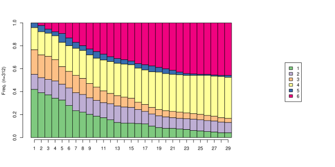
Figure 1: Decoded states of the HMM with $k=5$ hidden states and dropout state (6th pink)

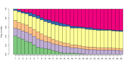
(a) Not treated

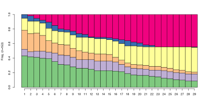
(b) Treated

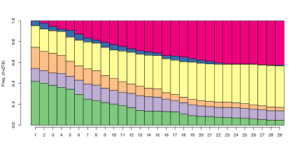
(c) Gender: Female

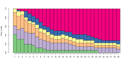
(d) Gender: Male

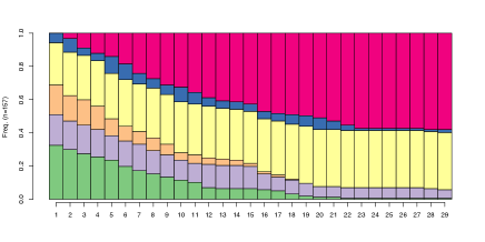
(e) Old

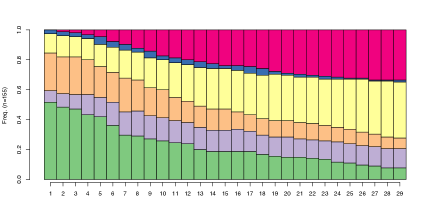
(f) Young

Figure 2: Decoded states of the proposed HMM with respect to the covariates: drug use, gender, and age; the legend for the states is the same as that provided in Figure 1: green 1st, violet 2nd, orange 3rd, yellow 4th, blue 5th, and pink 6th (dropout state)

Interestingly, from Figure 1 we notice that it is possible to predict the survival curve for all patients by looking at the curve referred to the dropout state (the pink line). We recall that this decoding is provided using the estimated posterior probabilities which are directly provided by the proposed EM algorithm once the HMM with covariates is estimated. From these estimated survival curves, we conclude that drug use was not particularly effective in prolonging survival, males have a higher risk of dying compared to females, especially from the eighth visit, and older patients have a higher risk of dying compared to younger patients from the beginning of the study.

7 Conclusions

In this paper we extend maximum likelihood estimation of a finite mixture model (FMM) of Gaussian distributions with missing at random (MAR) responses to the hidden Markov model (HMM) for continuous multivariate longitudinal data. Considering that in this context dropout typically occurs due to the early termination from the trial, we include an extra absorbing state in the model so that this type of missing is informative. Overall, the proposed approach accounts for three types of missing data: the first two are intermittent and correspond to the situation of completely or partially missing responses for a given occasion, while the third type of missing data corresponds to dropout. We implement an exact maximum likelihood inferential approach to deal with the first two types of missingness, under the MAR approach. Estimation is carried out by an extended Expectation-Maximization algorithm implemented to account for missing values and to include an extra hidden state for the dropout. This inferential approach is also developed to estimate the parameters of the model when individual covariates are included in the distribution of the latent process. In such a context, it may be of interest to evaluate the effect of these covariates on the transition toward the dropout state. We notice that in the presence of missing data, the proposed approach also allows us to perform a sort of multiple imputation so as to predict the missing responses conditionally or unconditionally to the assigned latent state.

The simulation study allowed us to conclude that the model parameters are properly estimated even with a relatively large proportion of missing responses and dropout. The application to multivariate data about primary biliary cholangitis referred to several biochemical measurements of liver function turned out to be particularly challenging. The data were very sparse due to missing visits of the patients and the fact that some variables were not collected at each visit. Moreover, several dropouts occurred due to death. With the proposed approach, we identified five groups of patients differing for the severity of this rare disease and their transitions across states and towards the dropout state over time. According to the available covariates, it was possible to predict the distributions of survival times for groups of patients through the decoded states.

References

- Akaike, (1973) Akaike, H. (1973). Information theory as an extension of the maximum likelihood principle. In Petrov, B. N. and F., C., editors, Second International symposium on information theory, pages 267–281, Budapest. Akademiai Kiado.
- Albert et al., (2002) Albert, P., Follmann, D. A., Wang, S. A., and Suh, E. B. (2002). A latent autoregressive model for longitudinal binary data subject to informative missingness. Biometrics, 58:631–642.
- Albert, (2000) Albert, P. S. (2000). A transitional model for longitudinal binary data subject to nonignorable missing data. Biometrics, 56:602–608.
- Anderson, (2003) Anderson, T. (2003). An Introduction to Multivariate Statistical Analysis. Wiley Series in Probability and Statistics. Wiley.
- Bacci et al., (2014) Bacci, S., Pandolfi, S., and Pennoni, F. (2014). A comparison of some criteria for states selection in the latent Markov model for longitudinal data. Advances in Data Analysis and Classification, 8:125–145.
- Banfield and Raftery, (1993) Banfield, J. D. and Raftery, A. E. (1993). Model-based Gaussian and non-Gaussian clustering. Biometrics, pages 803–821.
- Bartolucci and Farcomeni, (2009) Bartolucci, F. and Farcomeni, A. (2009). A multivariate extension of the dynamic logit model for longitudinal data based on a latent Markov heterogeneity structure. Journal of the American Statistical Association, 104:816–831.
- (8) Bartolucci, F. and Farcomeni, A. (2015a). A discrete time event-history approach to informative drop-out in mixed latent markov models with covariates. Biometrics, 71:80–89.
- (9) Bartolucci, F. and Farcomeni, A. (2015b). Information matrix for hidden Markov models with covariates. Statistics and Computing, 25:515–526.
- Bartolucci et al., (2013) Bartolucci, F., Farcomeni, A., and Pennoni, F. (2013). Latent Markov Models for Longitudinal Data. Chapman & Hall/CRC Press, Boca Raton, FL.
- Bartolucci et al., (2014) Bartolucci, F., Farcomeni, A., and Pennoni, F. (2014). Latent Markov models: A review of a general framework for the analysis of longitudinal data with covariates. TEST, 23:433–465.
- Bartolucci et al., (2017) Bartolucci, F., Pandolfi, S., and Pennoni, F. (2017). LMest: An R package for latent Markov models for longitudinal categorical data. Journal of Statistical Software, 81:1–38.
- Baum et al., (1970) Baum, L., Petrie, T., Soules, G., and Weiss, N. (1970). A maximization technique occurring in the statistical analysis of probabilistic functions of Markov chains. Annals of Mathematical Statistics, 41:164–171.
- Bouveyron et al., (2019) Bouveyron, C., Celeux, G., Murphy, T. B., and Raftery, A. E. (2019). Model-based clustering and classification for data science: with applications in R. Cambridge University Press.
- Cox, (1972) Cox, D. R. (1972). Regression models and life-tables. Journal of the Royal Statistical Society: Series B, 34:187–202.
- Davison and Hinkley, (1997) Davison, A. C. and Hinkley, D. V. (1997). Bootstrap Methods and their Application. Cambridge University Press, Cambridge, MA.
- Delalleau et al., (2018) Delalleau, O., Courville, A., and Bengio, Y. (2018). Efficient EM training of Gaussian mixtures with missing data. arXiv preprint arXiv:1209.0521v2.
- Dempster et al., (1977) Dempster, A. P., Laird, N. M., and Rubin, D. B. (1977). Maximum likelihood from incomplete data via the EM algorithm (with discussion). Journal of the Royal Statistical Society, Series B, 39:1–38.
- Di Zio et al., (2007) Di Zio, M., Guarnera, U., and Luzi, O. (2007). Imputation through finite Gaussian mixture models. Computational Statistics & Data Analysis, 51:5305–5316.
- Dickson et al., (1989) Dickson, E. R., Grambsch, P. M., Fleming, T. R., Fisher, L. D., and Langworthy, A. (1989). Prognosis in primary biliary cirrhosis: model for decision making. Hepatology, 10:1–7.
- Diggle and Kenward, (1994) Diggle, P. and Kenward, M. G. (1994). Informative drop-out in longitudinal data analysis. Journal of the Royal Statistical Society, Series C, 43:49–93.
- Diggle et al., (2002) Diggle, P. J., Heagerty, P., Liang, K.-Y., and Zeger, S. L. (2002). Analysis of Longitudinal Data. Oxford University Press, New York.
- Eirola et al., (2014) Eirola, E., Lendasse, A., Vandewalle, V., and Biernacki, C. (2014). Mixture of Gaussians for distance estimation with missing data. Neurocomputing, 131:32–42.
- Fitzmaurice et al., (2004) Fitzmaurice, G. M., Laird, N. M., and Ware, J. H. (2004). Applied longitudinal analysis. Wiley-Interscience, Hoboken, NJ.
- Follmann and Wu, (1995) Follmann, D. and Wu, M. (1995). An approximate generalized linear model with random effects for informative missing data. Biometrics, 51:151–168.
- Henderson et al., (2000) Henderson, R., Diggle, P., and Dobson, A. (2000). Joint modelling of longitudinal measurements and event time data. Biostatistics, 1:465–480.
- Hsiao, (2005) Hsiao, C. (2005). Analysis of Panel Data. Cambridge University Press, New York.
- Hsieh et al., (2006) Hsieh, F., Tseng, Y.-K., and Wang, J.-K. (2006). Joint modeling of survival and longitudinal data: likelihood approach revisited. Biometrics, 62:1037–1043.
- Hunt and Jorgensen, (2003) Hunt, L. and Jorgensen, M. (2003). Mixture model clustering for mixed data with missing information. Computational Statistics & Data Analysis, 41(3-4):429–440.
- Juang and Rabiner, (1991) Juang, B. and Rabiner, L. (1991). Hidden Markov models for speech recognition. Technometrics, 33:251–272.
- Kenward et al., (2003) Kenward, M. G., Molenberghs, G., and Thijs, H. (2003). Pattern-mixture models with proper time dependence. Biometrika, 90:53–71.
- Lange et al., (2015) Lange, J. M., Hubbard, R. A., Inoue, L. Y. T., and Minin, V. N. (2015). A joint model for multistate disease processes and random informative observation times, with applications to electronic medical records data. Biometrics, 71:90–101.
- Little, (1994) Little, R. J. (1994). A class of pattern-mixture models for normal incomplete data. Biometrika, 81:471–483.
- Little, (1995) Little, R. J. A. (1995). Modeling the drop-out mechanism in repeated-measures studies. Journal of the American Statistical Association, 90:1112–1121.
- Little and Rubin, (2020) Little, R. J. A. and Rubin, D. B. (2020). Statistical Analysis with Missing Data. John Wiley Sons Hoboken NJ.
- Marino and Alfò, (2020) Marino, M. F. and Alfò, M. (2020). Finite mixtures of hidden Markov models for longitudinal responses subject to drop out. Multivariate behavioral research, 55:647–663.
- Maruotti, (2015) Maruotti, A. (2015). Handling non-ignorable dropouts in longitudinal data: A conditional model based on a latent Markov heterogeneity structure. TEST, 24:84–109.
- McLachlan and Peel, (2000) McLachlan, G. and Peel, D. (2000). Finite Mixture Models. Wiley.
- Molenberghs et al., (1997) Molenberghs, G., Kenward, M. G., and Lesaffre, E. (1997). The analysis of longitudinal ordinal data with nonrandom drop-out. Biometrika, 84:33–44.
- Molenberghs and Verbeke, (2000) Molenberghs, G. and Verbeke, G. (2000). Linear mixed models for longitudinal data. Springer.
- Montanari and Pandolfi, (2018) Montanari, G. E. and Pandolfi, S. (2018). Evaluation of long-term health care services through a latent Markov model with covariates. Statistical Methods & Applications, 27:151–173.
- Murtaugh et al., (1994) Murtaugh, P. A., Dickson, E. R., Van Dam, G. M., Malinchoc, M., Grambsch, P. M., Langworthy, A. L., and Gips, C. H. (1994). Primary biliary cirrhosis: prediction of short-term survival based on repeated patient visits. Hepatology, 20:126–134.
- Nylund-Gibson and Choi, (2018) Nylund-Gibson, K. and Choi, A. Y. (2018). Ten frequently asked questions about latent class analysis. Translational Issues in Psychological Science, 4(4):440.
- Oakes, (1999) Oakes, D. (1999). Direct calculation of the information matrix via the EM algorithm. Journal of the Royal Statistical Society, Series B, 61:479–482.
- R Core Team, (2021) R Core Team (2021). R: A Language and Environment for Statistical Computing. R Foundation for Statistical Computing, Vienna, Austria.
- Rizopoulos, (2010) Rizopoulos, D. (2010). JM: An R package for the joint modelling of longitudinal and time-to-event data. Journal of Statistical Software, 35:1–33.
- Rizopoulos, (2012) Rizopoulos, D. (2012). Joint models for longitudinal and time-to-event data: With applications in R. CRC press.
- Rubin, (1976) Rubin, D. B. (1976). Inference and missing data. Biometrika, 63:581–592.
- Schwarz, (1978) Schwarz, G. (1978). Estimating the dimension of a model. Annals of Statistics, 6:461–464.
- Spagnoli et al., (2011) Spagnoli, A., Henderson, R., Boys, R., and Houwing-Duistermaat, J. (2011). A hidden Markov model for informative dropout in longitudinal response data with crisis states. Statistics & Probability Letters, 81:730–738.
- Titterington et al., (1985) Titterington, D. M., Smith, A. F. M., and E., M. U. (1985). Statistical analysis of Finite Mixture Distributions. John Wiley, New York.
- Vermunt et al., (1999) Vermunt, J. K., Langeheine, R., and Böckenholt, U. (1999). Discrete-time discrete-state latent Markov models with time-constant and time-varying covariates. Journal of Educational and Behavioral Statistics, 24:179–207.
- Viterbi, (1967) Viterbi, A. (1967). Error bounds for convolutional codes and an asymptotically optimum decoding algorithm. IEEE Transactions on Information Theory, 13:260–269.
- Welch, (2003) Welch, L. R. (2003). Hidden Markov models and the Baum-Welch algorithm. IEEE Information Theory Society Newsletter, 53:1–13.
- Wulfsohn and Tsiatis, (1997) Wulfsohn, M. and Tsiatis, A. (1997). A joint model for survival and longitudinal data measured with error. Biometrics, 53:330–339.
- Zhang et al., (2020) Zhang, W., Xie, F., and Tan, J. (2020). A robust joint modeling approach for longitudinal data with informative dropouts. Computational Statistics, 35:1759–1783.
- Zhou et al., (2020) Zhou, T., Daniels, M. J., and Müller, P. (2020). A semiparametric bayesian approach to dropout in longitudinal studies with auxiliary covariates. Journal of Computational and Graphical Statistics, 29:1–12.
- Zucchini et al., (2016) Zucchini, W., MacDonald, I. L., and Langrock, R. (2016). Hidden Markov Models for Time Series: An Introduction using R, volume 150. CRC press, Boca Raton, FL.