A Sample-Based Taylor’s Theorem for Density Estimation

Taylor from Samples for Density Estimation

A Statistical Taylor Theorem
and Extrapolation of Truncated Densities

Abstract

We show a statistical version of Taylor’s theorem and apply this result to non-parametric density estimation from truncated samples, which is a classical challenge in Statistics [Woo85, Stu93]. The single-dimensional version of our theorem has the following implication: “For any distribution $P$ on $[0,1]$ with a smooth log-density function, given samples from the conditional distribution of $P$ on $[a,a+\varepsilon]\subset[0,1]$, we can efficiently identify an approximation to $P$ over the whole interval $[0,1]$, with quality of approximation that improves with the smoothness of $P$.”

To the best of knowledge, our result is the first in the area of non-parametric density estimation from truncated samples, which works under the hard truncation model, where the samples outside some survival set $S$ are never observed, and applies to multiple dimensions. In contrast, previous works assume single dimensional data where each sample has a different survival set $S$ so that samples from the whole support will ultimately be collected.

1 Introduction

Non-parametric density estimation is a well-developed field in Statistics and Machine Learning [Was06, Tsy08a] with applications to many scientific areas including economics [AF10, LR07], and survival analysis [Woo85]. A central challenge in this field is estimating a probability density function $\mathcal{P}(\boldsymbol{x})$ from samples, without making strong parametric assumptions about the density. Of course, this is quite challenging as $\mathcal{P}$ may exhibit very rich behavior which might be difficult or information theoretically impossible to discern given a finite number of samples. Thus, to make the task feasible at all, some constraints are placed on $\mathcal{P}$, typically in the form of smoothness, which allows estimators to interpolate among the observed samples. Indeed, a prominent method for non-parametric density estimation is based on kernels [WJ94, BGK10, Sim12, Sco15], whose usual interpolating estimate takes the form $\hat{\mathcal{P}}(\boldsymbol{x})={\frac{1}{n}}\sum_{i=1}^{n}k(\boldsymbol{x}_{i};\boldsymbol{x})$, for some kernel function $k(\cdot;\cdot)$, where $\boldsymbol{x}_{1},\ldots,\boldsymbol{x}_{n}$ are the observations from $\mathcal{P}$. In some settings it is also preferable to use kernels to estimate the log-density function [CS06]. Even with smoothness assumptions, the problem is challenging enough information theoretically, that the achievable error takes the form $O(n^{-r/(r+d)})$, under various norms, where $d$ is the dimension and $r$ is the assumed order of smoothness of $\mathcal{P}$ [McD17a, LR07, BGvdM92].

Despite the fact that both kernel based and histogram based estimators achieve the optimal consistency rates, their estimators do not have a form that is appealing for other statistical uses. For example, if our goal is to do inference as well then it would be helpful if the estimated distribution is represented as a member of an exponential family [Ney37, Goo63, SFG⁺17]. A parallel line of research has hence devoted in exponential series estimators of non-parametric densities, starting with the celebrated work of Barron and Sheu [BS91] which was later extended to multidimensional settings by [Wu10]. Our work follows this line of research and the estimators that we compute are always members of some exponential family.

The goal of this paper is to extend this literature from the traditional interpolating regime to the much more challenging extrapolating regime. In particular, we consider settings wherein we are constrained to observe samples of $\mathcal{P}$ in a subset of its support, yet we want to procure estimates $\hat{\mathcal{P}}$ that approximate $\mathcal{P}$ over its entire support. This question problem is motivated by truncated statistics, another well-developed field in Statistics and Econometrics [Coh91, Hec76, Mad87, BSH93], which targets statistical estimation in settings where the samples are truncated depending on their membership in some set. Truncation may occur for several reasons, ranging from measurement device saturation effects to data collection practices, bad experimental design, ethical or privacy considerations that disallow the use of some data, etc.

Non-parametric density estimation from truncated samples is well-studied problem in statistics with many applications in economics and survival analysis [PM84, Woo85, LY91, Stu93, Gaj88, LY91]. However, due to the very challenging nature of this problem, all the previous works on this topic consider only a soft truncation model that does not completely hide some part of the support but only decreases the probability of observing samples that lie in the truncation set. In particular, each sample $\boldsymbol{x}_{i}$ from $\mathcal{P}$ also samples a truncation set $S_{i}$ which then determines whether this sample is truncated or not. As a result, samples from the entire support are ultimately collected, thus the unknown density can be interpolated, with some appropriate re-weighting, from those samples covering the entire support. Moreover, the existing work only targets single-dimensional densities despite the importance of non-parametric estimation in multiple dimensions as we discussed above.

In this work, our goal is to solve the seemingly impossible problem of estimating a non-parametric density, even in parts of the support where we do not observe any sample! More precisely, we consider the more standard, in truncated statistics, hard truncation model, wherein there is a fixed set $S$ that determines whether a sample from $\mathcal{P}$ is truncated. We solve this problem under slightly stronger, but similar, assumptions to the ones used in the vanilla non-parametric density estimation problems. At the same time, we extend the non-parametric density estimation from truncated samples to multi-dimensional settings, which is a significant generalization of the existing work.

Our main theorems, summarized in Section 1.1, can be interpreted as a statistical version of Taylor’s theorem, which allows us to use truncated samples from some sufficiently smooth density $\mathcal{P}$ and extrapolate from these samples an estimate $\hat{\mathcal{P}}$ which approximates $\mathcal{P}$ on its entire support. The statistical rates achieved by our theorems are slightly worse but comparable to those known in non-parametric density estimation under untruncated samples, i.e., in the interpolating regime. It is an interesting open problem whether we can improve the novel extrapolation rates that we provide in this work, to match exactly the interpolation rates of the vanilla non-parametric density estimation.

From a technical point of view, a central challenge that we face is to bound the extrapolation error of multivariate polynomial approximation, which is a challenging problem and is a subject of active area of research. Our main technical contribution is to show a novel way to prove strong bounds on the extrapolation error of our algorithms invoking only well-studied anti-concentration theorems, which is of independent interest and we believe that it will have applications beyond truncated statistics. More precisely, one of our main technical results is a “Distortion of Conditioning” lemma (Lemma 4.5), providing a tight relationship between the $\ell_{1}$ distance between two exponential families as computed under conditioning on different subsets of the support. As we said, this lemma is proven using probabilistic techniques, and provides a viable route to prove our statistical Taylor result in high dimensions, where polynomial approximation theory techniques do not appear sufficient.

Further Related Work. The use of exponential series estimators in non-parametric density estimation problems has many applications in other important problems in statistics, e.g., entropy estimation problems [BRH11, WGW13], estimation of copula functions [CFT06], and online density estimation [GK17]. We believe that our results and tools can be a cornerstone in extending these results to their truncated statistics counterparts.

Despite its long history, the field of truncated statistics suffers from a lack of computationally and statistically efficient estimators in high-dimensions. Recent work, has made progress towards rectifying these limitations in parametric settings such as multi-variate normal estimation, linear regression, logistic regression, and support estimation [DGTZ18, DGTZ19, KTZ19, IZC20, CDS20]. Roughly speaking, this recent progress exploits the strong parametric assumptions about the density that is being estimated to extrapolate the density outside of the truncation set. In comparison to this work, our goal here is to remove these parametric assumptions, allowing a very broad family of distributions to be extrapolated from truncated samples.

1.1 Our Results and Techniques

In this work we provide provable extrapolation of non-parametric density functions from samples, i.e., given samples from the conditional density on some subset $S$ of the support, we recover the shape of the density function outside of $S$. We consider densities proportional to $e^{f(x)}$, where $f$ is a sufficiently smooth function. Our observation consists of samples from a density proportional to $\mathds{1}_{S}(x)e^{f(x)}$, where $S$ is a known (via a membership oracle) subset of the support. For this problem to even be well-posed we need further assumptions on the density function. Even if we are given the exact conditional density $\mathds{1}_{S}(x)e^{f(x)}$, it is easy to see that, if $f\notin C_{\infty}$, i.e., if $f$ is not infinitely times differentiable everywhere in the whole support, there is no hope to extrapolate its curve outside of $S$; for a simple example, if we observe a density proportional to $e^{|x|}$ truncated in $(-\infty,0]$ we cannot extrapolate this density to $(0,+\infty)$, because we cannot distinguish whether we are observing truncated samples from $e^{-x}$ or $e^{|x|}$. On the other hand, if the log-density $f$ is analytic and sufficiently smooth, then the value of $f$ at every $x$ can be determined only from local information, namely its derivatives at a single point. This well known property of analytic functions is quantified by Taylor’s remainder theorem. In this work we build on this and show that, even given samples from a sufficiently smooth density and even if these samples are conditioned in a small subset of the support, we can still determine the function in the entire support and most importantly this can be done in a statistically and computationally efficient way.

Since it is impossible to extrapolate non-smooth densities, we restrict our attention to smooth functions $f$. In particular, we assume that the $r$-th order derivatives of $f$ increase at most exponentially in $r$, i.e., $|f^{(r)}(\boldsymbol{x})|\leq M^{r}$ for some $M\in\mathbb{R}_{+}$ and all $\boldsymbol{x}$ (see Definition 2.4). Notice that similar assumptions are standard in the interpolation regime of non-parametric density estimation [BS91, Wu10].

We start our exposition with the single-dimensional version of our extrapolation problem in Section 3. In this setting it is easier to compare with the existing line of work on non-parametric density estimation both in the vanilla non-truncated and in the truncated setting. Moreover, in the single-dimensional setting, we are able to show a slightly stronger information theoretic result. We assume that there exists some unknown log-density function $f$, a known set $S$, and we observe samples from the distribution $\mathcal{P}(f,S)$, which has density proportional to $\mathds{1}_{S}(x)e^{f(x)}$. Our goal is to estimate the whole distribution $\mathcal{P}(f)$. For simplicity we assume that $f$ is supported on $[0,1]$ and hence $S\subseteq[0,1]$. Our first step is to consider the semi-parametric class of densities $p$ that consists of polynomial series that can approximate the unknown non-parametric log-density $f$. Then we truncate this polynomial series and we only consider densities of the form $e^{p(x)}$, where $p$ is a degree $k$ polynomial, with large enough $k$; observe that these densities belong to an exponential family.

Our first result is that the polynomial which maximizes the likelihood with respect to the conditional distribution $\mathcal{P}(f,S)$ (we call this polynomial the “MLE polynomial”) approximates the density $e^{f(x)}$ everywhere on $[0,1]$, i.e. the MLE polynomial has small extrapolation error.

Definition 1.1 (MLE polynomial).

For some log-density $f:\mathbb{R}\mapsto\mathbb{R}$ denote $\mathcal{P}(f,S)$ the truncated distribution on $S$ with density function $\mathcal{P}(f,S;x)=\mathds{1}_{S}(x)e^{f(x)}/\int_{S}e^{f(x)}dx$. We define the MLE polynomial $p^{\ast}$ of degree $k$ with respect to $\mathcal{P}(f,S)$ as

$$p^{\ast}=\operatorname*{argmax}_{p:\deg(p)\leq k}\operatorname*{\mathbf{E}}_{x\sim\mathcal{P}(f,S)}[\log(\mathcal{P}(p,S;x))]\,.$$

The extrapolation guarantee for the MLE polynomial cannot follow from the fact that, for example, the Taylor polynomial extrapolates, because the MLE polynomial and the Taylor polynomial are in principle very different. It is not hard to argue that the MLE polynomial of sufficiently large degree has small interpolation error: it approximates well the density inside $S$. In our result we show that the same polynomial has small extrapolation error and hence approximates the density on the entire interval $[0,1]$.

Informal Theorem 1 (MLE Extrapolation Error, Theorem 3.1).

Let $\mathcal{P}(f,[0,1])$ be a probability distribution with sufficiently smooth log-density $f$ and let $\mathcal{P}(f,S)$ be its conditional distribution on $S\subset[0,1]$. The MLE w.r.t $\mathcal{P}(f,S)$ polynomial $p^{*}$ of degree $O(\log(1/\epsilon))$ satisfies $\mathrm{d}_{\mathrm{TV}}(\mathcal{P}(f,[0,1]),\mathcal{P}(p^{*},[0,1]))\leq\epsilon$.

Extending this result to multivariate densities is significantly more challenging. The reason is that multivariate polynomial interpolation is much more intricate and is a subject of active research, see for example the survey [GS00]. Instead of trying to characterize the properties of the exact MLE polynomial we give an alternative method for obtaining multivariate extrapolation guarantees that does not rely on multivariate polynomial interpolation. Our approach uses the assumption that the set $S$ has non-trivial volume, i.e., $\mathrm{vol}(S)\geq\alpha$ for some $\alpha>0$. Observe that this assumption is not needed in the single dimensional sample complexity analysis; in the multi-dimensional setting we need this assumption even to analyze the population model.

Informal Theorem 2 (Multivariate MLE Extrapolation Error, Theorem 4.2).

Let $\mathcal{P}(f,[0,1]^{d})$ be a probability distribution with sufficiently smooth log-density $f$ and let $\mathcal{P}(f,S)$ be its conditional distribution on $S\subset[0,1]^{d}$ with $\mathrm{vol}(S)\geq\alpha$. The MLE w.r.t $\mathcal{P}(f,S)$ polynomial $p^{*}$ of degree $O(d^{3}/\alpha^{2}+\log(1/\epsilon))$ satisfies $\mathrm{d}_{\mathrm{TV}}(\mathcal{P}(f,[0,1]^{d}),\mathcal{P}(p^{*},[0,1]^{d}))\leq\epsilon$.

To prove 2 we use a structural result that quantifies the distortion of the metric space of exponential families under conditioning. Given a polynomial $p$ with corresponding density $\mathcal{P}(p,[0,1]^{d})$ we consider the conditioning map that maps $\mathcal{P}(p,[0,1]^{d})$ to the distribution $\mathcal{P}(p,S)$. We show that conditioning distorts the total variation by a factor less than $(d/\alpha)^{O(k)}$, i.e., distributions that are close in the image of the conditioning map are also close in the domain and vice versa.

Informal Theorem 3 (Distortion of Conditioning, Lemma 4.5).

Let $p,q$ be polynomials of degree at most $k$. For every $S\subseteq[0,1]^{d}$ with $\mathrm{vol}(S)\geq\alpha$ it holds

$$\left(d/\alpha\right)^{-O(k)}\leq\frac{\mathrm{d}_{\mathrm{TV}}(\,\mathcal{P}(p,[0,1]^{d}),\ \mathcal{P}(q,[0,1]^{d})\,)}{\mathrm{d}_{\mathrm{TV}}(\mathcal{P}(p,S),\ \mathcal{P}(q,S))}\leq\left(d/\alpha\right)^{O(k)}.$$

Using the above theorem, our strategy for showing 2 is illustrated in Figure 1 and is as follows. Our first step is to use Taylor’s remainder theorem to prove that there exists a polynomial $p$, associated with $f$, such that both $\mathrm{d}_{\mathrm{TV}}(\mathcal{P}(p,S),\mathcal{P}(f,S))$ and $\mathrm{d}_{\mathrm{TV}}(\mathcal{P}(p,[0,1]^{d}),$ $\mathcal{P}(f,[0,1]^{d}))$ are very small when $p$ has sufficiently large degree. Next, we show that, by optimizing the likelihood function on $S$ over the space of degree $k$ polynomials, we obtain the MLE polynomial $q$ which achieves very small total variation distance to $f$ on $S$, i.e. $\mathrm{d}_{\mathrm{TV}}(\mathcal{P}(q,S),\mathcal{P}(f,S))$ is also small. Hence, from the triangle inequality we have that $\mathrm{d}_{\mathrm{TV}}(\mathcal{P}(q,S),\mathcal{P}(p,S))$ is also very small. The next step, which is the crucial one, is that we can now apply our novel 3 to obtain that $\mathrm{d}_{\mathrm{TV}}(\mathcal{P}(q,[0,1]^{d}),\mathcal{P}(p,[0,1]^{d}))$ blows up at most by a factor of $(d/\alpha)^{O(k)}$. This argument leads to an upper bound on the extrapolation error ($y$ in Figure 1). The last key observation is that the quantity $\mathrm{d}_{\mathrm{TV}}(\mathcal{P}(p,S),\mathcal{P}(f,S))$ decreases faster than $(d/\alpha)^{-O(k)}$ as the degree $k$ increases and hence we can make the extrapolation error arbitrarily small by choosing sufficiently high degree.

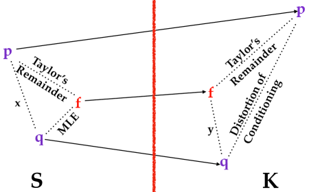
Figure 1: Using 3 to show the extrapolation guarantees of MLE. $K=[0,1]^{d}$. $p$ is the Taylor Polynomial of $f$: from Taylor’s remainder theorem we know that, in both $S$ and $K$, $p$ is very close to $f$. $q$ is the MLE polynomial on $S$: it is very close to $f$ in $S$. The distance $x$ is bounded by triangle inequality. The distance of $p$ and $q$ in $K$ is upper bounded by $x\ (d/\alpha)^{O(k)}$ by  3. Finally, $y$ is the extrapolation error of the MLE polynomial $q$ on $K$ and is bounded by another triangle inequality. Overall, $y\leq\mathrm{d}_{\mathrm{TV}}(\mathcal{P}(f,K),\mathcal{P}(p,K))+(d/\alpha)^{O(k)}x\leq\mathrm{d}_{\mathrm{TV}}(\mathcal{P}(f,K),\mathcal{P}(p,K))+(d/\alpha)^{O(k)}(\mathrm{d}_{\mathrm{TV}}(\mathcal{P}(f,S),\mathcal{P}(p,S))+\mathrm{d}_{\mathrm{TV}}(\mathcal{P}(f,S),\mathcal{P}(q,S)))$.

So far we have argued about the extrapolation error of the population MLE polynomial, i.e., we assume that we have access to the population distribution $\mathcal{P}(f,S)$ and that we can maximize the population MLE with no error. Our next step is to show how we can incorporate the statistical error from the access to only finitely many samples from $\mathcal{P}(f,S)$ and to provide an efficient algorithm that computes the MLE polynomial with small enough approximation loss.

Informal Theorem 4 (Extrapolation Algorithm: Theorem 4.1).

Let $\mathcal{P}(f,[0,1]^{d})$ be sufficiently smooth. Let $S\subseteq[0,1]^{d}$ be such that $\mathrm{vol}(S)\geq\alpha$. There exists an algorithm that draws

$$N=2^{\widetilde{O}(d^{4}/\alpha^{2})}\cdot(1/\epsilon)^{O(d+\log(1/\alpha))}$$

samples from $\mathcal{P}(f,S)$, runs in time polynomial in the number of samples, and with probability at least $99\%$ finds a polynomial $q$ of degree $\widetilde{O}(d^{3}/\alpha^{2})+O(\log(1/\epsilon))$ such that $\mathrm{d}_{\mathrm{TV}}(\mathcal{P}(f,[0,1]^{d}),\mathcal{P}(q,[0,1]^{d}))\leq\epsilon$.

It is well known that non-parametric density estimation (in the interpolation regime, i.e. from untruncated samples) under smoothness assumptions requires samples that depend exponentially in the dimension, i.e. the typical rate is $(1/\epsilon)^{\Theta(d)}$, see for example [Tsy08b], [McD17b]. The usual assumption is that the density has bounded derivatives, i.e. it belongs to a Sobolev or Besov space. Our problem of extrapolating the density function is a strict generalization of non-parametric density estimation and therefore our sample complexity naturally scales as $(1/\epsilon)^{O(d+\log(1/\alpha))}$, where the $\log(1/\alpha)$ reflects the impact of conditioning on a small volume set $S$. In particular, for sets of constant volume, in low dimensions, we obtain a sample complexity that is polynomial in $1/\epsilon$.

2 Definitions and Preliminaries

Notation. Let $K\subseteq\mathbb{R}^{d}$ and $B\in\mathbb{R}_{+}$, we define $L_{\infty}(K,B)$ to be the set of all functions $f:K\to\mathbb{R}$ such that $\max_{\boldsymbol{x}\in K}\left|f(\boldsymbol{x})\right|\leq B$. We may use $L_{\infty}(B)$ instead of $L_{\infty}([0,1]^{d},B)$. We also define $\mathrm{diam}_{p}(K)=\sup_{\boldsymbol{x},\boldsymbol{y}\in K}\left\|\boldsymbol{x}-\boldsymbol{y}\right\|_{p}$ where $\left\|\cdot\right\|_{p}$ is the usual $\ell_{p}$-norm of vectors. Let $\mathbb{R}^{d\times\cdots\text{($k$ times)}\cdots\times d}$ be the set of $k$-order tensors of dimension $d$, which for simplicity we will denote by $\mathbb{R}^{d^{k}}$. For $\boldsymbol{\alpha}\in\mathbb{N}^{d}$, we define the factorial of the multi-index $\boldsymbol{\alpha}$ to be $\boldsymbol{\alpha}!=(\alpha_{1}!)\cdots(\alpha_{d}!)$. Additionally for any $\boldsymbol{x},\boldsymbol{y},\boldsymbol{z}\in\mathbb{R}^{d}$ we define $\boldsymbol{z}^{\boldsymbol{\alpha}}=z_{1}^{\alpha_{1}}\cdots z_{d}^{\alpha_{d}}$ and in particular $(\boldsymbol{x}-\boldsymbol{y})^{\boldsymbol{\alpha}}=(x_{1}-y_{1})^{\alpha_{1}}\cdots(x_{d}-y_{d})^{\alpha_{d}}$.

Remark 2.1.

Throughout the paper, for simplicity of exposition, we will consider the support $K$ of the densities that we aim to learn to be the hypercube $[0,1]^{d}$. Our results hold for arbitrary convex sets with the following property $[a,b]^{d}\subseteq K\subseteq[c,d]^{d}$. Then all our results will be modified by multiplying with a function of $R\triangleq\frac{d-c}{b-a}$.

2.1 Multivariate Polynomials

When we use a polynomial to define a probability distribution, as we will see in Section 2.4, the constant term of the polynomial has to be determined from the rest of the coefficients so that the resulting function integrates to $1$. For this reason we can ignore the constant term. A polynomial $q:\mathbb{R}^{d}\to\mathbb{R}$ is a function of the form

$$q(\boldsymbol{x})=\sum_{\boldsymbol{\alpha}\in\mathbb{N}^{d},0<\left|\boldsymbol{\alpha}\right|\leq k}v_{\boldsymbol{\alpha}}\boldsymbol{x}^{\boldsymbol{\alpha}}$$ (2.1)

where $v_{\boldsymbol{\alpha}}\in\mathbb{R}$. The monomials of degree $\leq k$ can be indexed by a multi-index $\boldsymbol{\alpha}\in\mathbb{N}^{d}$ with $\left|\boldsymbol{\alpha}\right|\leq k$ and any polynomial belongs to the vector space defined by the monomials as per eq. 2.1.

To associate the space of polynomials with a Euclidean space we can use any ordering of monomials, for example, the lexicographic ordering. Using this ordering we can define the monomial profile of degree $k$, $\boldsymbol{m}_{k}:\mathbb{R}^{d}\to\mathbb{R}^{t_{k}-1}$, as $\left(\boldsymbol{m}_{k}(\boldsymbol{x})\right)_{\boldsymbol{\alpha}}=\boldsymbol{x}^{\boldsymbol{\alpha}}$ where $t_{k}=\binom{d+k}{k}$ is equal to the number of monomials with $d$ variables and degree at most $k$ and where we abuse notation to index a coordinate in $\mathbb{R}^{t_{k}-1}$ via a multi-index $\boldsymbol{\alpha}\in\mathbb{N}^{d}$ with $\left|\boldsymbol{\alpha}\right|\leq k$ and $\boldsymbol{\alpha}\neq\boldsymbol{0}$; this can be formally done using the lexicographic ordering. Therefore the vector space of polynomials is homomorphic to the vector space $\mathbb{R}^{t_{k}-1}$ via the following correspondence

$$\boldsymbol{v}\in\mathbb{R}^{t_{k}-1}\leftrightarrow\boldsymbol{v}^{T}\boldsymbol{m}_{k}(\boldsymbol{x})\triangleq q_{\boldsymbol{v}}(\boldsymbol{x}).$$ (2.2)

We denote by $\mathcal{Q}_{d,k}$ the space of polynomials of degree at most $k$ with $d$ variables and zero constant term, where we might drop $d$ from the notation if it is clear from context.

2.2 High-order Derivatives and Taylor’s Theorem

In this section we will define the basic concepts about high order derivatives of a multivariate real-valued function $f:K\to\mathbb{R}$, where $K\subseteq\mathbb{R}^{d}$.

Fix $k\in\mathbb{N}$ and let $\boldsymbol{u}\in[d]^{k}$. We define the order $k$ derivative of $f$ with index $\boldsymbol{u}=(u_{1},\dots,u_{k})$ as $\mathbf{D}^{k}_{\boldsymbol{u}}f(\boldsymbol{x})=\frac{\partial^{k}f}{\partial x_{u_{1}}\cdots\partial x_{u_{k}}}(\boldsymbol{x})$, observe that $\mathbf{D}^{k}_{\boldsymbol{u}}f$ is a function from $K$ to $\mathbb{R}$. The order $k$ derivative of $f$ at $\boldsymbol{x}\in S$ is then the tensor $\mathbf{D}^{k}f(\boldsymbol{x})\in\mathbb{R}^{d^{k}}$ where the entry of $\mathbf{D}^{k}f(\boldsymbol{x})$ that corresponds to the index $\boldsymbol{u}\in[d]^{k}$ is $(\mathbf{D}^{k}f(\boldsymbol{x}))_{\boldsymbol{u}}=\mathbf{D}^{k}_{\boldsymbol{u}}f(\boldsymbol{x})$. Due to symmetry the $k$-th order derivatives can be indexed with a multi-index $\boldsymbol{\alpha}\triangleq(\alpha_{1},\dots,\alpha_{d})\in\mathbb{N}^{d}$, with $\left|\boldsymbol{\alpha}\right|=\sum_{i=1}^{d}\alpha_{i}=k$, as follows $\mathbf{D}_{\boldsymbol{\alpha}}f(\boldsymbol{x})=\frac{\partial^{\left|\boldsymbol{\alpha}\right|}f}{\partial^{\alpha_{1}}x_{1}\cdots\partial^{\alpha_{d}}x_{d}}(\boldsymbol{x})$. Observe that the $k$-order derivative of $f$ is a function $\mathbf{D}^{k}f:K\to\mathbb{R}^{d^{k}}$.

Norm of High-order Derivative. There are several ways to define the norm of the tensor and hence the norm of a $k$-order derivative of a multi-variate function. Here we will define only the norm that we will use in the rest of the paper as follows

$$\left\|\mathbf{D}^{k}f\right\|_{\infty}\triangleq\sup_{\boldsymbol{x}\in K}\max_{\boldsymbol{u}\in[d]^{k}}\left|\mathbf{D}^{k}_{\boldsymbol{u}}f(\boldsymbol{x})\right|=\sup_{\boldsymbol{x}\in K}\max_{\boldsymbol{u}\in[d]^{k}}\left|\frac{\partial^{k}f}{\partial x_{u_{1}}\cdots\partial x_{u_{k}}}(\boldsymbol{x})\right|.$$ (2.3)

Observe that this definition depends on $K$, but for ease of notation we eliminate $K$ from the notation and we make sure that this set will be clear from the context. For most part of the paper $K$ is the box $[0,1]^{d}$. We next define the $k$-order Taylor approximation of a multi-variate function.

Definition 2.2.

(Taylor Approximation) Let $f:K\to\mathbb{R}$ be a $(k+1)$-times differentiable function on the convex set $K\subseteq\mathbb{R}^{d}$. Then we define $\overline{f}_{k}(\cdot;\boldsymbol{x})$ to be the $k$-order Taylor approximation of $f$ around $\boldsymbol{x}$ as follows $\overline{f}_{k}(\boldsymbol{y};\boldsymbol{x})=\sum_{\boldsymbol{\alpha}\in\mathbb{N}^{d},\left|\boldsymbol{\alpha}\right|\leq k}\frac{\mathbf{D}_{\boldsymbol{\alpha}}f(\boldsymbol{x})}{\boldsymbol{\alpha}!}(\boldsymbol{y}-\boldsymbol{x})^{\boldsymbol{\alpha}}$.

We are now ready to state the main application of Taylor’s Theorem. For the proof of this theorem together with the statement of the multi-dimensional Taylor’s Theorem we refer to Appendix A.

Theorem 2.3 (Corollary of Taylor’s Theorem).

Let $K\subseteq\mathbb{R}^{d}$ and $f:K\to\mathbb{R}$ be a $(k+1)$-times differentiable function such that $\mathrm{diam}_{\infty}(K)\leq R$ and $\left\|\mathbf{D}^{k+1}f\right\|_{\infty}\leq W$, then for any $\boldsymbol{x},\boldsymbol{y}\in K$ it holds that $\left|f(\boldsymbol{y})-\overline{f}_{k}(\boldsymbol{y};\boldsymbol{x})\right|\leq\left(15d/k\right)^{k+1}\cdot R^{k+1}\cdot W.$

2.3 Bounded and High-order Smooth Functions

In this section we define the set of functions that our statistical Taylor theorem applies. It is also the domain of function with respect to which we are solving the non-parametric truncated density estimation problem. This set of functions is very similar to the functions consider for interpolation of probability densities from exponential families [BS91]. We note that in this paper our goal is to solve a much more difficult problem since our goal is to do extrapolation instead of interpolation. We call the set of function that we consider bounded and high-order smooth functions.

Definition 2.4 (Bounded and High-order Smooth Functions).

Let $K=[0,1]^{d}$, we define the set $\mathcal{L}(B,M)$ of functions $f:K\to\mathbb{R}$ for which the following conditions are satisfied.

1. (Bounded Value) It holds that $\max_{\boldsymbol{x}\in K}\left|f(\boldsymbol{x})\right|\leq B$.

2. (High-Order Smoothness) For any natural number $k$ with $k\geq k_{0}$, $f$ is $k$-times continuously differentiable and it holds that $\left\|\mathbf{D}^{k}f\right\|_{\infty}\leq M^{k}$.

We note that the definition of the class $\mathcal{L}$ depends on $k_{0}$ as well but for ease of notation we don’t keep track of this dependence and we treat $k_{0}$ as a constant throughout the paper.

2.4 Probability Distributions

We are now ready to define probability distributions with a given log-density function.

Definition 2.5.

Let $S\subseteq\mathbb{R}^{d}$ and let $f:S\to\mathbb{R}$ such that $\int_{S}\exp(f(\boldsymbol{x}))d\boldsymbol{x}<\infty$. We define the distribution $\mathcal{P}(f,S)$ with log-density $f$ supported on $S$ to be the distribution with density

$$\mathcal{P}(f,S;\boldsymbol{x})=\frac{\mathds{1}_{S}(\boldsymbol{x})\ e^{f(\boldsymbol{x})}}{\int_{S}e^{f(\boldsymbol{x})}\ \mathrm{d}x}=\mathds{1}_{S}(\boldsymbol{x})\ \exp(f(\boldsymbol{x})-\psi(f,S))\,,~{}~{}~{}~{}\text{where}~{}~{}~{}\psi(f,S)=\log\int_{S}e^{f(x)}\mathrm{d}\boldsymbol{x}\,.$$

If $f$ is equal to a $k$ degree polynomial $q_{\boldsymbol{v}}\in\mathcal{Q}_{k}$ with coefficients $\boldsymbol{v}\in\mathbb{R}^{t_{k}-1}$, where $t_{k}=\binom{d+k}{k}$, then instead of $\mathcal{P}(q_{\boldsymbol{v}},S)$ we write $\mathcal{P}(\boldsymbol{v},S)$. Finally, let $T\subseteq S$, we define $\mathcal{P}(f,S;T)=\int_{T}\mathcal{P}(f,S;\boldsymbol{x})\mathrm{d}\boldsymbol{x}$.

Our main focus in this paper is on probability distributions $\mathcal{P}(f,[0,1]^{d})$ where $f\in\mathcal{L}(B,M)$ for some known parameters $B,M$. More specifically our main goal is to approximation the density of $\mathcal{P}(f,[0,1]^{d})$ given samples from $\mathcal{P}(f,S)$, where $S$ is a measurable subset of $[0,1]^{d}$.

3 Single Dimensional Densities

In this section we show our Statistical Taylor Theorem for single-dimensional densities. We keep this analysis separate from our main multi-dimensional theorem for several reasons. First, there exists a great body of work on single-dimensional non-parametric estimation problems in the vanilla setting and more specifically in truncated estimation problems this is the only setting that has been considered so far. Therefore, it is easier to compare the estimators and results that we get with the existing results. In fact this is the strategy that is followed in other multi-dimensional non-parametric estimation problems, e.g., see [Wu10]. Another reason is that in the single dimensional setting we are able to obtain a slightly stronger information theoretic result using more elementary tools, although the analysis of our efficient algorithmic procedure is the same as in multiple dimensions. Finally, the single dimensional setting serves as a nice example where the difference between interpolation and extrapolation is more clear.

In this section our goal is to estimate the density of the distribution $\mathcal{P}(f,[0,1])$ using only samples from $\mathcal{P}(f,S)$, where the log-density $f$ is a bounded and high-order smooth function, i.e. $f\in\mathcal{L}(B,M)$, and $S$ is a measurable subset of $[0,1]$. As a first step we need to understand what is a sufficient degree for a polynomial to well-approximate (Section 3.1) this is the part that is different compared to the multi-dimensional case that we present in Section 4. In Section 3.2 we state the application of our general multi-dimensional statistical and computational result to the single dimensional case where the assumptions and guarantees have a simpler form.

3.1 Identifying the Sufficient Degree

In this section we assume population access to $\mathcal{P}(f,S)$ and our goal is to identify a polynomial $q$ such that $\mathcal{P}(q,[0,1])$ approximates $\mathcal{P}(f,[0,1])$. In particular, we want to answer the question: if $q$ minimizes the KL-divergence between $\mathcal{P}(q,S)$ and $\mathcal{P}(f,S)$, what can we say about the total variation distance between $\mathcal{P}(q,[0,1])$ and $\mathcal{P}(f,[0,1])$? Moreover, how does this depend on the degree of $q$? As the degree of $q$ grows, it certainly allows $\mathcal{P}(q,S)$ to come closer to $\mathcal{P}(f,S)$. The natural thing to expect hence is that the same is true of $\mathcal{P}(q,[0,1])$, coming closer to $\mathcal{P}(f,[0,1])$. Unfortunately, this is not necessarily the case, because it could be that, as the degree of the polynomial increases, the approximant $\mathcal{P}(q,S)$ overfits to $\mathcal{P}(f,S)$, so extrapolating to $[0,1]$ fails to give a good approximation to $\mathcal{P}(f,[0,1])$. This is the main technical difficulty of this section.

In the next theorem, we show is that if the function is high-order smooth, then there is some threshold beyond which we get better approximations using higher degrees, i.e. overfitting does not happen for any degree above some threshold. We illustrate this behavior in Example 3.2.

Theorem 3.1 (MLE Polynomial Extrapolation Error).

Let $I=[0,1]\subseteq\mathbb{R}$ and $f:I\mapsto\mathbb{R}$ be a function that is $(k+1)$-times continuously differentiable on $I$, with $\left|f^{(k+1)}(x)\right|\leq M^{k+1}$ for all $x\in I$. Let $S\subseteq I$ be a measurable set such that $\mathrm{vol}(S)>0$, and $p$ be a polynomial of degree at most $k$ defined as $p=\operatorname*{argmin}_{q\in\mathcal{Q}_{k}}\mathrm{D}_{\mathrm{KL}}(\mathcal{P}(f,S)\|\mathcal{P}(q,S))\,.$ Then, it holds that $\mathrm{D}_{\mathrm{KL}}(\mathcal{P}(f,I)\|\mathcal{P}(p,I))\leq e^{W_{k}}W_{k}^{2}$ where $W_{k}=\frac{M^{k+1}}{(k+1)!}\,.$

The proof of Theorem 3.1 can be found in Section B.1. We also note that we can prove a more general version of Theorem 3.1 where $I$ is any interval $[a,b]$. The difference in the guarantees is that the term $W_{k}$ will be multiplied by $R^{k+1}$ where $R\triangleq b-a$.

To convey the motivation for our theorem and illustrate its guarantees, we use the following example.

Example 3.2.

Let $f(x)=\sin(10\cdot x)$ and $S=[0,1/2]$. Our goal is to estimate the probability distribution $\mathcal{P}(f,[0,1])$ using only samples from $\mathcal{P}(f,S)$. The guarantees of Theorem 3.1 are illustrated in Figure 2 where we can see the density of the distributions $\mathcal{P}(f,[0,1])$, $\mathcal{P}(f,S)$, $\mathcal{P}(q,S)$ and $\mathcal{P}(q,[0,1])$ for various values of the degree of $q$, where $q$ is always chosen to minimize the KL-divergence between $\mathcal{P}(f,S)$ and $\mathcal{P}(q,S)$, i.e., using no further information about $\mathcal{P}(f,[0,1])$. As we see, $\mathcal{P}(q,S)$ approximates $\mathcal{P}(f,S)$ very well for all the presented degrees, with a marginal improvement as the degree of $q$ is increased.

An important observation is that the approximation error between $\mathcal{P}(f,[0,1])$ and $\mathcal{P}(q,[0,1])$ is not monotone in any range of degrees of $q$. In particular, when the degree of $q$ is $10$ then $\mathcal{P}(q,[0,1])$ is reasonably close to $\mathcal{P}(f,[0,1])$ while when the (degree of $q$) $=12$ then $\mathcal{P}(q,[0,1])$ is way off. This suggests that overfitting occurs for degree $=12$. The point of Theorem 3.1 is that it guarantees that, for degree greater than a threshold, overfitting cannot happen and $\mathcal{P}(q,[0,1])$ will always be a good approximation to $\mathcal{P}(f,[0,1])$.

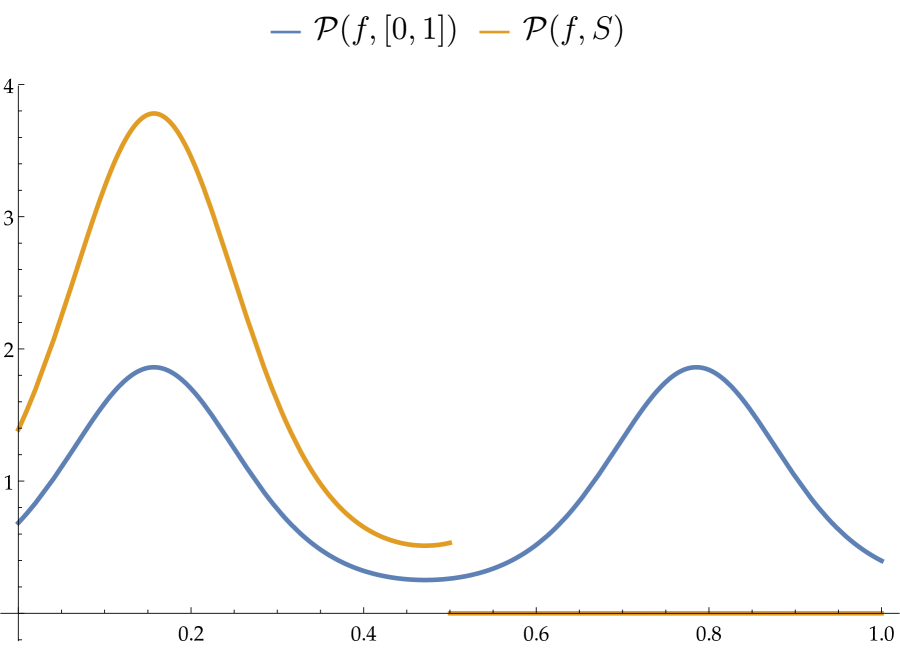
(a) The densities of $\mathcal{P}(f,[0,1])$ and $\mathcal{P}(f,S)$.

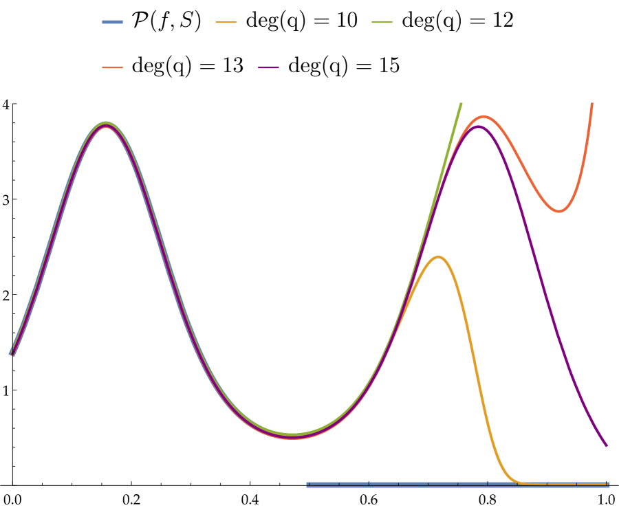
(b) $\mathcal{P}(f,S)$ and normalized on $S$ functions $e^{q(\cdot)}$ for different $\mathrm{deg}(q)$.

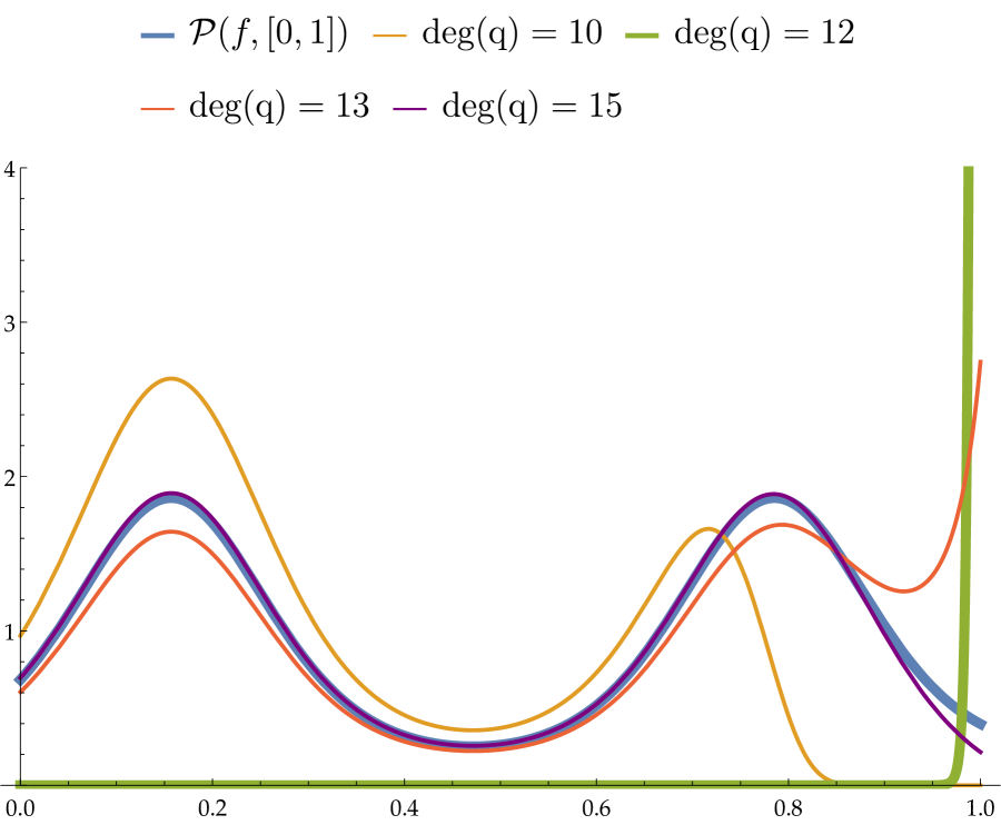
(c) The densities of $\mathcal{P}(f,[0,1])$ and $\mathcal{P}(q,[0,1])$ for different $\mathrm{deg}(q)$.

Figure 2: In figure (a) we can see the probability density functions of the distributions $\mathcal{P}(f,[0,1])$ and $\mathcal{P}(f,S)$. In figure (b) we have the density of $\mathcal{P}(f,S)$ together with the functions $\exp(q(x))$ for various degrees of $q$ normalized so that the integral on $S$ is 1. As we can see all the degrees approximate very well the conditional density but they have completely different behavior outside $S$. In figure (c) we can see the densities $\mathcal{P}(f,[0,1])$ and $\mathcal{P}(q,[0,1])$ for various degrees of $q$. The difference between (b) and (c) is that in (c) the functions are normalized so that their integral over $[0,1]$ is equal to $1$ whereas in (b) the integral over $S$ is equal to $1$.

3.2 Handling the Optimization Error

Our next theorem handles the approximation error that is introduced, due to access to finite samples.

Theorem 3.3 (Approximate MLE Polynomial Extrapolation Error).

Let $I=[0,1]$, $f\in\mathcal{L}(B,M)$ be a function supported on $I$, $S\subseteq I$ be a measurable set such that $\mathrm{vol}(S)\geq\alpha$, $D_{k}$ be the convex set $D_{k}=\{p\in\mathcal{Q}_{k}:p\in L_{\infty}(I,3B)\}\,$, where $k=\Omega(M+\log(1/\epsilon))$, and let also $r^{*}_{k}=\min_{p\in D_{k}}\mathrm{D}_{\mathrm{KL}}(\mathcal{P}(f,S)\|\mathcal{P}(p,S))$. If some $q$ with $q\in D_{k}$ satisfies

$$\mathrm{D}_{\mathrm{KL}}(\mathcal{P}(f,S)\|\mathcal{P}(q,S))\leq r_{k}^{*}+2^{-O(k\log(1/\alpha)+B)},$$ (3.1)

then it holds that $\mathrm{d}_{\mathrm{TV}}(\mathcal{P}(f,I),\mathcal{P}(q,I))\leq\epsilon$.

The proof of Theorem 3.3 can be found in Section B.2. Next we argue that we can efficiently compute a polynomial $q$ that satisfies Equation 3.1. Unfortunately, the proof of this step is not simplified in the 1-D case and we need to invoke our general multi-dimensional theorem with the assumptions and guarantees simplified due to the single dimensionality of the distribution. For more details about the specific algorithm that we use we refer to Section 4.2. This leads to the following theorem.

Theorem 3.4 (1-D Statistical Taylor Theorem).

Let $I=[0,1]$, $f\in\mathcal{L}(B,M)$ be a function supported on $I$, and $S\subseteq I$ be a (measurable) subset of $I$ such that $\mathrm{vol}(S)\geq\alpha$. There exists an algorithm that draws $N=2^{\widetilde{O}((M+\log(1/\epsilon))\log(1/\alpha)+B)}$ samples from $\mathcal{P}(f,S)$, runs in time polynomial in the number of samples, and outputs a vector of coefficients $\boldsymbol{v}$ such that $\mathrm{d}_{\mathrm{TV}}(\mathcal{P}(f,K),\mathcal{P}(q_{\boldsymbol{v}},K))\leq\epsilon$.

Proof.

We define the convex set $D_{k}=\left\{\boldsymbol{v}\in\mathbb{R}^{m}~{}:~{}\max_{\boldsymbol{x}\in[0,1]^{d}}\left|\boldsymbol{v}^{T}\boldsymbol{m}_{k}(\boldsymbol{x})\right|\leq 3B\right\}$, where $m=\binom{d+k}{k}-1$. From Theorem 3.3 we can fix $k=O(M+\log(1/\epsilon))$ and find a candidate $\boldsymbol{v}$ such that $\mathrm{D}_{\mathrm{KL}}(\mathcal{P}(f,S)\|\mathcal{P}(q_{\boldsymbol{v}},S))\leq\min_{\boldsymbol{u}\in D_{k}}\mathrm{D}_{\mathrm{KL}}(\mathcal{P}(f,S)\|\mathcal{P}(q_{\boldsymbol{u}},S))+2^{-O(k\log(1/\alpha)+B)}$. Therefore, from Theorem 4.7 we obtain that with $N=2^{\widetilde{O}(k\log(1/\alpha)+B)}$ samples and in time $\mathrm{poly}(N)$, we can compute such a candidate. ∎

4 Multi-Dimensional Densities

In this section we show the general form of our Statistical Taylor Theorem that applies to multi-dimensional densities. Although the techniques used in this section and involved and possibly of independent interest, our strategy to prove this theorem is similar to the strategy that we followed in Section 3: (1) we identify the sufficient degree that we need to use, (2) we handle approximation errors that we get as a result of finite sample, and (3) we design an efficient algorithm to compute the solutions that are information-theoretically shown to exist. This leads to our main theorem.

Theorem 4.1 (Multi-Dimensional Statistical Taylor Theorem).

Let $f:[0,1]^{d}\to\mathbb{R}$ with $f\in\mathcal{L}(B,M)$ and $S\subseteq[0,1]^{d}$ such that $\mathrm{vol}(S)\geq\alpha$. Let $k=\widetilde{\Omega}(d^{3}M/\alpha^{2}+B)+2\log(1/\epsilon)$, then there exists an algorithm that uses $N$ samples from $\mathcal{P}(f,S)$ with

$$N=2^{\widetilde{O}(d^{4}M/\alpha^{2}+Bd)}\cdot(1/\epsilon)^{O(d+\log(1/\alpha))},$$

runs in $\mathrm{poly}(N)$ time and outputs a vector $\boldsymbol{v}$ such that $\mathrm{d}_{\mathrm{TV}}(\mathcal{P}(f,K),\mathcal{P}(q_{\boldsymbol{v}},K))\leq\epsilon$.

The main bottleneck in the proof of the above theorem is that in the multi-dimensional polynomial interpolation theory there are no sufficient tools to prove the extrapolation properties of an estimator that can be computed efficiently. Our formulation of the extrapolation problem in the language of density estimation enables us to use anti-concentration results to prove extrapolation results for polynomial approximations. In particular, we prove our main lemma which we call “Distortion of Conditioning Lemma” which we believe is of independent interest.

4.1 Identifying the Sufficient Degree – The Distortion of Conditioning Lemma

The goal of this section is to identify the sufficient degree so that the MLE polynomial approximates well the true density in the whole domain $K=[0,1]^{d}$, i.e., it has small extrapolation error.

Theorem 4.2 (Multivariate MLE Polynomial Extrapolation Error).

Let $K=[0,1]^{d}\subseteq\mathbb{R}^{d}$, $f\in\mathcal{L}(B,M)$ be function supported on $K$, and $S\subseteq K$ be a measurable subset of $K$ such that $\mathrm{vol}(S)\geq\alpha$. Moreover, define $k=\widetilde{\Omega}\left(\frac{d^{3}M}{\alpha^{2}}+\log\left(\frac{2^{B}}{\epsilon}\right)\right)$, $D=\{\boldsymbol{v}:\max_{\boldsymbol{x}\in K}\left|\boldsymbol{v}^{T}\boldsymbol{m}_{k}(\boldsymbol{x})\right|\leq 3B\}$, Moreover, let $r^{*}_{k}=\min_{\boldsymbol{u}\in D}\mathrm{D}_{\mathrm{KL}}(\mathcal{P}(f,S)\|\mathcal{P}(\boldsymbol{u},S))$. Then, for every $\boldsymbol{u}\in D$ such that $\mathrm{D}_{\mathrm{KL}}(\mathcal{P}(f,S)\|\mathcal{P}(\boldsymbol{u},S))\leq r^{*}_{k}+e^{-\widetilde{\Omega}\left(\frac{d^{3}M}{\alpha^{2}}+B\right)}\cdot\left(\frac{1}{\epsilon}\right)^{-\Omega(\log(d/\alpha))}\,,$ it holds that $\mathrm{d}_{\mathrm{TV}}(\mathcal{P}(f,K),\mathcal{P}(\boldsymbol{u},K))\leq\epsilon$.

The first step in proving Theorem 4.2 is to understand the approximation error as a function of the degree that we use when we have access to the population distribution $\mathcal{P}(f,S)$. This is established in the following lemma whose proof can be found in Section C.1.

Lemma 4.3 (Approximation of Log-density).

Let $K\subseteq\mathbb{R}^{d}$ be a convex set centered at the origin $\boldsymbol{0}$ of diameter $\mathrm{diam}_{\infty}(K)\leq R$ and let $f\in\mathcal{L}(B,M)$ be a function supported on $K$. There exists polynomial $p(\boldsymbol{x})=\boldsymbol{v}^{T}\boldsymbol{m}_{k}(\boldsymbol{x})$ such that for every $S\subseteq K$ it holds $\mathrm{D}_{\mathrm{KL}}(\mathcal{P}(f,S)\|\mathcal{P}(\boldsymbol{v},S))\leq 2\left(\frac{15MRd}{k}\right)^{k+1}$ and $\left\|\mathds{1}_{K}p\right\|_{\infty}\leq 2B+\left(\frac{15MRd}{k}\right)^{k+1}.$

From Lemma 4.3 there exists $\boldsymbol{v}$ such that $\left\|\mathds{1}_{K}\boldsymbol{v}^{T}\boldsymbol{m}_{k}(\boldsymbol{x})\right\|_{\infty}\leq 2B+\left(15Md/k\right)^{k+1}$. Moreover, from the same lemma we have that $\min_{\boldsymbol{w}\in D}\mathrm{D}_{\mathrm{KL}}(\mathcal{P}(f,S)\|\mathcal{P}(\boldsymbol{w},S))\leq\mathrm{D}_{\mathrm{KL}}(\mathcal{P}(f,S)\|\mathcal{P}(\boldsymbol{v},S))\leq 2\left(15Md/k\right)^{k+1}$. To simplify notation set $r_{k}=2\left(15Md/k\right)^{k+1}$. Now, let $q(\boldsymbol{x})=\boldsymbol{u}^{T}\boldsymbol{m}_{k}(\boldsymbol{x})$ be any approximate minimizer in $D$ of the KL-divergence between $\mathcal{P}(q,S)$ and $\mathcal{P}(f,S)$ that satisfies

$$\mathrm{D}_{\mathrm{KL}}(\mathcal{P}(f,S)\|\mathcal{P}(\boldsymbol{u},S))\leq\min_{\boldsymbol{w}\in D}\mathrm{D}_{\mathrm{KL}}(\mathcal{P}(f,S)\|\mathcal{P}(\boldsymbol{w},S))+\overline{\epsilon}\leq r_{k}+\overline{\epsilon}.$$

From Pinsker’s inequality and the subadditivity of the square root we get: $\mathrm{d}_{\mathrm{TV}}(\mathcal{P}(f,S),\mathcal{P}(\boldsymbol{u},S))\leq\sqrt{r_{k}}+\sqrt{\overline{\epsilon}}$. Our next step is to relate the conditional total variation $\mathrm{d}_{\mathrm{TV}}(\mathcal{P}(f,S),\mathcal{P}(\boldsymbol{u},S))$ with the global total variation $\mathrm{d}_{\mathrm{TV}}(\mathcal{P}(f,K),\mathcal{P}(\boldsymbol{u},K))$. For this we develop a novel extrapolation technique based on anti-concentration of polynomial functions. In particular we use the following theorem.

Theorem 4.4 (Theorem 2 of [CW01]).

Let $K=[0,1]^{d}$ and let $p:\mathbb{R}^{d}\mapsto\mathbb{R}$ be a polynomial of degree at most $k$. If $q\geq 1$, then there exists a constant $C$ such that for any $\gamma>0$ it holds $\left(\int_{K}|p(\boldsymbol{x})|^{q/k}\mathrm{d}\boldsymbol{x}\right)^{1/q}\int_{K}\mathds{1}\{|p(\boldsymbol{x})|\leq\gamma\}\mathrm{d}\boldsymbol{x}\leq C\gamma^{1/k}~{}\min(q,d)\,.$

This result is crucial for extrapolation because it can be used to bound the behavior of a polynomial function even outside the region from which we get the samples. This is the main idea of the following lemma which is one of the main technical contributions of the paper and we believe that it is of independent interest.

Lemma 4.5 (Distortion of Conditioning).

Let $K=[0,1]^{d}$ and let $p,q$ be polynomials of degree at most $k$ such that $p,q\in L_{\infty}(K,B)$. There exists absolute constant $C>0$ such that for every $S\subseteq K$ with $\mathrm{vol}(S)>0$ it holds

$$e^{-2B}\mathrm{vol}(S)~{}\leq\frac{\mathrm{d}_{\mathrm{TV}}(\mathcal{P}(p,K),\mathcal{P}(q,K))}{\mathrm{d}_{\mathrm{TV}}(\mathcal{P}(p,S),\mathcal{P}(q,S))}\leq~{}8e^{5B}\frac{(2C\min(d,2k))^{k}}{\mathrm{vol}(S)^{k+1}}\,.\,$$

Remark 4.6.

Both Theorem 4.4 and Lemma 4.5 hold for the more general case where $K$ is an arbitrary convex subset of $\mathbb{R}^{d}$. We choose to state this weaker expression for ease of notation.

Unfortunately it is still not clear how to apply Lemma 4.5 because it assumes that both distributions that we are comparing have as log-density a bounded degree polynomial. Nevertheless, we can use a sequence of triangle inequalities together with Taylor’s Theorem (see Theorem 2.3) to combine Lemma 4.5 and Lemma 4.5 from which we can prove Theorem 4.2 as we explain in detail in Section C.3. The proof of the Distortion of Conditioning Lemma is presented in Section C.2.

4.2 Computing the MLE

In this section we describe an efficient algorithm that solves the Maximum Likelihood problem that we need in order to apply Theorem 4.2. We solve the following problem: given sample access to the conditional distribution $\mathcal{P}(f,S)$ and some fixed degree $k$, our algorithm finds a polynomial $p$ of degree $k$ that approximately minimizes the divergence $\mathrm{D}_{\mathrm{KL}}(\mathcal{P}(f,S)\|\mathcal{P}(\boldsymbol{u},S))$.

Theorem 4.7.

Let $f:[0,1]^{d}\to\mathbb{R}$ and $S\subseteq[0,1]^{d}$ with $\mathrm{vol}(S)\geq\alpha$. Fix a degree $k\in\mathbb{N}$, a parameter $C>0$, and define $D=\{\boldsymbol{v}~{}:~{}\max_{\boldsymbol{x}\in[0,1]^{d}}|\boldsymbol{v}^{T}\boldsymbol{m}_{k}(\boldsymbol{x})|\leq C\}$. There exists an algorithm that draws $N=2^{O(dk)}(C^{2}/\epsilon)^{2}$ samples from $\mathcal{P}(f,S)$, runs in time $2^{O(dk+C)}/(\alpha\epsilon^{2})$, and outputs $\hat{\boldsymbol{v}}\in D$ such that $\mathrm{D}_{\mathrm{KL}}(\mathcal{P}(f,S)\|\mathcal{P}(\hat{\boldsymbol{v}},S))\leq\min_{\boldsymbol{u}\in D}\mathrm{D}_{\mathrm{KL}}(\mathcal{P}(f,S)\|\mathcal{P}(\boldsymbol{u},S))+\epsilon$, with probability at least $99\%$.

The algorithm that we use for proving Theorem 4.7 is Projected Stochastic Gradient Descent with projection set $D$. In order to prove the guarantees of Theorem 4.7 we have to prove: (1) an upper bound on the number of steps that the PSGD algorithm needs, (2) find an efficient procedure to project to the set $D$. For the latter we can use the celebrated algorithm by Renegar for the existential theory of reals [Ren92a, Ren92b], as we explain in detail in Section C.4. To analyze PSGD we use the following lemma.

Lemma 4.8 (Theorem 14.8 of [SSBD14]).

Let $R,\rho>0$. Let $f$ be a convex function, $D\subseteq\mathbb{R}^{d}$ be a convex set of bounded diameter, $\mathrm{diam}_{2}(D)\leq R$, and let $\boldsymbol{w}^{*}\in\operatorname*{argmin}_{\boldsymbol{w}\in D}f(\boldsymbol{w})$. Consider the following Projected Gradient Descent (PSGD) update rule $\boldsymbol{w}_{t+1}=\mathrm{proj}_{D}(\boldsymbol{w}_{t}-\eta\boldsymbol{v}_{t})$, where $\boldsymbol{v}_{t}$ is an unbiased estimate of $\nabla f(\boldsymbol{w})$. Assume that PSGD is run for $T$ iterations with $\eta=\sqrt{R^{2}\rho^{2}/T}$. Assume also that for all $t$, $\left\|\boldsymbol{v}_{t}\right\|_{2}\leq\rho$ with probability $1$. Then, for any $\epsilon>0$, in order to achieve $\operatorname*{\mathbf{E}}[f(\overline{\boldsymbol{w}})]-f(\boldsymbol{w}^{*})\leq\epsilon$ it suffices that $T\geq R^{2}\rho^{2}/\epsilon^{2}$.

From the above lemma we can see that it remains to find an upper bound on the diameter of the set $D$ and an upper bound on the norm of the stochastic gradient $\left\|\boldsymbol{v}_{t}\right\|$. The latter follows from some algebraic calculations whereas the first one from tight bounds on the coefficients of a polynomial with bounded values [BBGK18]. For the full proof of Theorem 4.7, see Section C.4.

4.3 Putting Everything Together – The Proof of Theorem 4.1

From Theorem 4.2 we have that if we fix the degree $k=O(d^{3}M/\alpha^{2}+B)+2\log(1/\epsilon)$ then it suffices to optimize the function $L(\boldsymbol{v})$ of Equation C.5 constrained in the convex set $D=\left\{\boldsymbol{v}\in\mathbb{R}^{m}~{}:~{}\left\|\mathds{1}_{K}\boldsymbol{v}^{T}\boldsymbol{m}_{k}(\boldsymbol{x})\right\|_{\infty}\leq 3B\right\}.$ From Theorem 4.2 we have that a vector $\boldsymbol{v}$ with optimality gap $2^{-\widetilde{\Omega}(d^{3}M/\alpha^{2}+B)}(1/\epsilon)^{-\Omega(\log(d/\alpha)}$ achieves the extrapolation guarantee $\mathrm{d}_{\mathrm{TV}}(\mathcal{P}(f,K),\mathcal{P}(\boldsymbol{v}_{T},K))\leq\epsilon$. From Theorem 4.7 we have that there exists an algorithm that achieves this optimality gap with sample complexity $N=B^{2}2^{O(dk)}2^{\widetilde{O}(d^{3}M/\alpha^{2}+B)}(1/\epsilon)^{O(\log(d/\alpha))}=2^{\widetilde{O}(d^{4}M/\alpha^{2}+Bd)}(1/\epsilon)^{d+\log(1/\alpha)}\ .$

Appendix A Multidimensional Taylor’s Theorem

In this section we present the Taylor’s theorem for multiple dimensions and we prove Theorem 2.3. We remind the following notation from the preliminaries section $\boldsymbol{x}^{\boldsymbol{\alpha}}=x_{1}^{\alpha_{1}}\cdot x_{2}^{\alpha_{2}}\cdots x_{d}^{\alpha_{d}}$.

Theorem A.1 (Multi-Dimensional Taylor’s Theorem).

Let $S\subseteq\mathbb{R}^{d}$ and $f:S\to\mathbb{R}$ be a $(k+1)$-times differentiable function, then for any $\boldsymbol{x},\boldsymbol{y}\in S$ it holds that

$$f(\boldsymbol{y})=\sum_{\boldsymbol{\alpha}\in\mathbb{N}^{d},\left|\boldsymbol{\alpha}\right|\leq k}\frac{\mathbf{D}_{\boldsymbol{\alpha}}f(\boldsymbol{x})}{\boldsymbol{\alpha}!}(\boldsymbol{y}-\boldsymbol{x})^{\boldsymbol{\alpha}}+H_{k}(\boldsymbol{y};\boldsymbol{x}),~{}~{}~{}~{}\text{with}$$

$$H_{k}(\boldsymbol{y};\boldsymbol{x})=\sum_{\boldsymbol{\beta}\in\mathbb{N}^{d},\left|\boldsymbol{\beta}\right|=k+1}R_{\boldsymbol{\beta}}(\boldsymbol{y};\boldsymbol{x})(\boldsymbol{y}-\boldsymbol{x})^{\boldsymbol{\beta}}~{}~{}\text{and}~{}~{}R_{\boldsymbol{\beta}}(\boldsymbol{y};\boldsymbol{x})=\frac{\left|\boldsymbol{\beta}\right|}{\boldsymbol{\beta}!}\int_{0}^{1}(1-t)^{\left|\boldsymbol{\beta}\right|-1}\mathbf{D}_{\boldsymbol{\beta}}f(\boldsymbol{x}+t(\boldsymbol{y}-\boldsymbol{x}))dt.$$

We now provide a proof of Theorem 2.3.

Proof of Theorem 2.3.

We start by observing that

$$\left|f(\boldsymbol{y})-\overline{f}_{k}(\boldsymbol{y};\boldsymbol{x})\right|\leq\left(\sum_{\boldsymbol{\beta}\in\mathbb{N}^{d},\left|\boldsymbol{\beta}\right|=k+1}\frac{1}{\boldsymbol{\beta}!}\right)\cdot R^{k+1}\cdot W.$$

This inequality follows from multidimensional Taylor’s Theorem by some simple calculations. Now to show wanted result it suffices to show that $\sum_{\boldsymbol{\beta}\in\mathbb{N}^{d},\left|\boldsymbol{\beta}\right|=k+1}\frac{1}{\boldsymbol{\beta}!}\leq\left(\frac{15d}{k}\right)^{k+1}$. To prove the latter we first show that $\min_{\boldsymbol{\beta}\in\mathbb{N}^{d},\left|\boldsymbol{\beta}\right|=k+1}\boldsymbol{\beta}!=(\ell!)^{d-r}((\ell+1)!)^{r}$ where $\ell=\lfloor\frac{k+1}{d}\rfloor$ and $r=k+1\pmod{d}$. We prove this via contradiction, if this is not true then the minimum $\min_{\boldsymbol{\beta}\in\mathbb{N}^{d},\left|\boldsymbol{\beta}\right|=k+1}\boldsymbol{\beta}!$ is achieved in multi-index $\boldsymbol{\beta}$ such that there exist $i,j\in[d]$ such that $\beta_{i}<\ell$ and $\beta_{j}>\ell+1$. In this case we define $\boldsymbol{\beta}^{\prime}$ to be equal to $\boldsymbol{\beta}$ except for $\beta^{\prime}_{i}=\beta_{i}+1$ and $\beta^{\prime}_{j}=\beta_{j}-1$. In this case we get $\boldsymbol{\beta}^{\prime}!<\frac{\beta_{j}}{\beta_{i}+1}\boldsymbol{\beta}^{\prime}!=\boldsymbol{\beta}!$, which contradicts the optimality of $\boldsymbol{\beta}$. Therefore we have that $\sum_{\boldsymbol{\beta}\in\mathbb{N}^{d},\left|\boldsymbol{\beta}\right|=k+1}\frac{1}{\boldsymbol{\beta}!}\leq\binom{d+k+1}{k+1}\frac{1}{((\ell+1)!)^{d}}$. Now via upper bounds from Stirling’s approximation we get that $\binom{d+k+1}{k+1}\frac{1}{((\ell+1)!)^{d}}\leq\frac{e^{k+1}\left(1+\frac{d}{k+1}\right)^{k+1}}{((k+1)/d)^{k+1}e^{-k-1}}\leq\left(\frac{e^{2}d}{k}\right)^{k+1}\left(1+\frac{k}{k+1}\right)^{k+1}$ and the Theorem follows from simple calculations on the last expression. ∎

Appendix B Missing Proofs for Single Dimensional Densities

In this section we provide the proof of the theorems presented in Section 3.

B.1 Proof of Theorem 3.1

We are going to use the following result that bounds the error of Hermite polynomial interpolation, wherein besides matching the values of the target function the approximating polynomial also matches its derivatives. The following theorem can be seen as a generalization of Lagrange interpolation, where the interpolation nodes are distinct, and Taylor’s remainder theorem where we find a polynomial that matches the first $k$ derivatives at a single node.

Lemma B.1 (Hermite Interpolation Error).

Let $x_{1},\ldots,x_{s}$ be distinct nodes in $[a,b]$ and let $m_{1},\ldots,m_{s}\in\mathbb{N}$ such that $\sum_{i=1}^{s}m_{i}=k+1$. Moreover, let $f$ be a $(k+1)$ times continuously differentiable function over $[a,b]$ and $p$ be a polynomial of degree at most $k$ such that for each $x_{i}$

$$p(x_{i})=f(x_{i})~{}~{}~{}p^{\prime}(x_{i})=f^{\prime}(x_{i})~{}~{}~{}\ldots~{}~{}~{}p^{(m_{i}-1)}(x_{i})=f^{(m_{i}-1)}(x_{i})\,.$$

Then for all $x\in[a,b]$, there exists $\xi\in(a,b)$ such that

$$f(x)-p(x)=\frac{f^{(k+1)}(\xi)}{(k+1)!}\prod_{i=1}^{s}(x-x_{i})^{m_{i}}\,.$$

We are also going to use the following upper bound on Kullback-Leibler divergence. For a proof see Lemma 1 of [BS91].

Lemma B.2.

Let $\mathcal{P},\mathcal{Q}$ be distributions on $\mathbb{R}$ with corresponding density functions $p,q$. Then for any $c>0$ it holds

$$\mathrm{D}_{\mathrm{KL}}(\mathcal{P}\|\mathcal{Q})\leq e^{\left\|\log(p(x)/q(x))-c\right\|_{\infty}}\int p(x)\left(\log\frac{p(x)}{q(x)}-c\right)^{2}\mathrm{d}x\,.$$

Before, the proof of Theorem 3.1 we are going to show a useful lemma. Let $f,g$ be two density functions such that $\mathrm{D}_{\mathrm{KL}}(f\|g)>0$ and let $r$ another function $r$ that lies strictly between the two densities $f,g$. The following lemma states that after we normalize $r$ to become a density function $\overline{r}$ we get that $\overline{r}$ is closer to $f$ in Kullback-Leibler divergence than $g$.

Lemma B.3 (Kullback-Leibler Monotonicity).

Let $f,g$ be density functions over $\mathbb{R}$ such that the measure defined by $f$ is absolutely continuous with respect to that defined by $g$, i.e. the support of $f$ is a subset of that of $g$. Let also $r$ be an integrable function such that $r(x)\geq 0$, for all $x\in\mathbb{R}$, and moreover, for all $x\in\mathbb{R}\setminus Z$

$$f(x)\leq r(x)<g(x)\quad\text{ or }\quad g(x)<r(x)\leq f(x)$$

where $Z$ is a set that has measure $0$ under both $f$ and $g$. Then, if $\overline{r}(x)=r(x)/\int r(x)\mathrm{d}x$ is the density function corresponding to $r(\cdot)$, it holds that

$$\mathrm{D}_{\mathrm{KL}}(f\|\overline{r})<\mathrm{D}_{\mathrm{KL}}(f\|g).$$

Proof.

To simplify notation we are going to assume that the support of $f$ is the entire $\mathbb{R}$, and we define the sets $A_{<}=\{x\in\mathbb{R}:r(x)<g(x)\}$, $A_{>}=\{x\in\mathbb{R}:r(x)>g(x)\}$. In the following proof we are going to ignore the measure zero set where the assumptions about $g,r,f$ do not hold. Denote $C=\int r(x)\mathrm{d}x=1-\int(g(x)-r(x))\mathrm{d}x$. We have

$$\mathrm{D}_{\mathrm{KL}}(f\|g)-\mathrm{D}_{\mathrm{KL}}(f\|\overline{r}) =\int f(x)\log\frac{\overline{r}(x)}{g(x)}\ \mathrm{d}x=\int f(x)\log\frac{r(x)}{g(x)}\ \mathrm{d}x-\log C$$

$$\geq\int r(x)\log\frac{r(x)}{g(x)}\ \mathrm{d}x-\log C\,,$$

where for the last inequality we used the fact that $f(x)<r(x)$ for all $x\in A_{<}$ and $f(x)>r(x)$ for all $x\in A_{>}$. Using the inequality $\log(1+z)\leq z$ we obtain $-\log C\geq\int(g(x)-r(x))\mathrm{d}x.$ Using this fact we obtain

$$\mathrm{D}_{\mathrm{KL}}(f\|p)-\mathrm{D}_{\mathrm{KL}}(f\|\overline{r}) \geq\int r(x)\log\frac{r(x)}{g(x)}\ \mathrm{d}x+\int(g(x)-r(x))\ \mathrm{d}x$$

$$\geq\int\left(r(x)\log\frac{r(x)}{g(x)}+g(x)-r(x)\right)\mathrm{d}x.$$

To finish the proof we observe that $r(x)\log(r(x)/g(x))+g(x)-r(x)>0$ for every $x$. To see this we rewrite the inequality as $\log\frac{r(x)}{g(x)}-1+\frac{g(x)}{r(x)}>0.$ To prove this we use the inequality $\log(z)-1+1/z>0$ for all $z\neq 1$. ∎

We are now ready to prove the main result of this section: Theorem 3.1.

Proof of Theorem 3.1

Recall that

$$p=\operatorname*{argmin}_{q\in\mathcal{Q}_{k}}\mathrm{D}_{\mathrm{KL}}(\mathcal{P}(f,S)\|\mathcal{P}(q,S))\,.$$

To simplify notation, we define the functions $\phi_{f}(x)=f(x)-\psi(f,S)$ and $\phi_{p}(x)=p(x)-\psi(p,S)$. Notice that these are the log densities of the conditional distributions $\mathcal{P}(f,S)$ and $\mathcal{P}(p,S)$ on the set $S$, viewed as functions over the entire interval $I$ (i.e. they are the conditional log densities without the indicator $\mathds{1}_{S}(x)$). Notice that $\phi_{p}$ is a polynomial of degree at most $k$. Let $g(x)=\phi_{f}(x)-\phi_{p}(x)$. We first show the following claim.

Claim B.4.

The equation $g(x)=0$ has at least $k+1$ roots in $S$, counting multiplicities.

Proof of B.4.

To reach a contradiction, assume that it has $k$ (or fewer) roots. Let $\xi_{1},\ldots,\xi_{s}\in I$ be the distinct roots of $g(x)=0$ ordered in increasing order and let $m_{1},\ldots,m_{s}$ be their multiplicities. Denote by $I_{0},\ldots,I_{s}$ the partition of $I$ using the roots of $g(x)$, that is

$$I_{0}=(-\infty,\xi_{1}]\cap I=[\xi_{0},\xi_{1}],\ I_{1}=[\xi_{1},\xi_{2}],\ \ldots,\ I_{s}=[\xi_{s},\xi_{s+1}]=[\xi_{s},+\infty)\cap I\,.$$

Let $q$ be the polynomial that has the same roots as $g(x)$ and also the same sign as $g(x)$ in every set $I_{j}$ of the partition. We claim that there exists $\lambda_{j}>0$ such that, for every $j$ and $x\in\mathrm{int}(I_{j})$, the expression $\phi_{f}(x)-(\phi_{p}(x)+\lambda q(x))$ has the same sign as $\phi_{f}(x)-\phi_{p}(x)$ and also $|\phi_{f}(x)-(\phi_{p}(x)+\lambda_{j}q(x))|<|\phi_{f}(x)-\phi_{p}(x)|$. Indeed, fix an interval $I_{j}$ and without loss of generality assume that $g(x)>0$ for all $x\in I_{j}\setminus\{\xi_{j},\xi_{j+1}\}$. Then it suffices to show that there exists $\lambda_{j}>0$ such that $0<g(x)-\lambda_{j}q(x)<g(x)$. Since $q(x)>0$ for every $x\in\mathrm{int}(I_{j})$, we need to choose $\lambda_{j}<g(x)/q(x)$. Since $\xi_{j}$ is a root of the same multiplicity of both $g(x)$ and $q(x)$ and $g(x),q(x)>0$ for all $x\in\mathrm{int}(I_{j})$ we have $\lim_{x\to\xi_{j}^{+}}\frac{g(x)}{q(x)}=a>0$. Similarly, we have $\lim_{x\to\xi_{j+1}^{-}}\frac{g(x)}{q(x)}=b>0$. We can now define the following function

$$h(x)=\begin{cases}a,&x=\xi_{j}\\ g(x)/q(x),&\xi_{j}<x<\xi_{j+1}\\ b,&x=\xi_{j+1}\end{cases}\,.$$

We showed that $h(x)$ is continuous in $I_{j}=[\xi_{j},\xi_{j+1}]$ and therefore has a minimum value $r_{j}>0$ in the closed interval $I_{j}$. We set $\lambda_{j}=r_{j}$. With the same argument as above we obtain that for each interval $I_{j}$ we can pick $\lambda_{j}>0$. Since the number of intervals in our partition is finite we may set $\lambda=\min_{j=0,\ldots,s}\lambda_{j}$ and still have $\lambda>0$.

We have shown that the polynomial $r(x)=\phi_{p}(x)+\lambda q(x)$ is almost everywhere, that is apart from a measure zero set, strictly closer to $\phi_{f}(x)$. In particular, we have that $\phi_{p}(x)$ for every $x\in[0,1]$, $|\phi_{f}(x)-r(x)|\leq|\phi_{f}(x)-\phi_{p}(x)|$ and for every $x\in S\setminus\{\xi_{0},\ldots,\xi_{s+1}\}$ it holds $|\phi_{f}(x)-r(x)|<|\phi_{f}(x)-\phi_{p}(x)|$. Moreover, by construction we have that $\phi_{f}(x)-r(x)$ and $\phi_{f}(x)-p(x)$ are always of the same sign. Finally, the degree of $r(x)$ is at most $k$. Using Lemma B.3 we obtain that $\mathrm{D}_{\mathrm{KL}}(\mathcal{P}(f,S)\|\mathcal{P}(r,S))<\mathrm{D}_{\mathrm{KL}}(\mathcal{P}(f,S)\|\mathcal{P}(p,S))$, which is impossible since we know that $p$ is the polynomial that minimizes the Kullback-Leibler divergence. ∎

We are now ready to finish the proof of our lemma. Using Lemma B.1 and B.4 we have that $\phi_{p}$ and $\phi_{f}$ are close not only in $S$ but in the whole interval $I$. In particular, for every $x\in I$ it holds

$$\left|f(x)-\log\int_{S}e^{f(x)}\mathrm{d}x-p(x)+\log\int_{S}e^{p(x)}\mathrm{d}x\right|\leq\frac{M}{(k+1)!}R^{k+1}:=W_{k}\,.$$ (B.1)

Using the above bound together with Lemma B.2, where we set $c=\log\frac{\psi(f,I)\psi(p,S)}{\psi(p,I)\psi(f,S)}$, we obtain

$$\mathrm{D}_{\mathrm{KL}}(\mathcal{P}(f,I)\|\mathcal{P}(p,I))\leq e^{W_{k}}W_{k}^{2}.$$

B.2 Proof of Theorem 3.3

We first show that the minimizer of the Kullback-Leibler divergence belongs to the set $D_{k}$. Let $q^{*}=\operatorname*{argmin}_{q\in\mathcal{Q}_{k}}\mathrm{D}_{\mathrm{KL}}(\mathcal{P}(f,S)\|\mathcal{P}(q,S))$ be the minimizer over the set of degree $k$ polynomials. From the assumption that $f\in L_{\infty}(I,B)$ we have that $e^{-B}\alpha\leq\int_{S}e^{f(x)}\mathrm{d}x\leq e^{B}$ and therefore $|\psi(f,S)|\leq B+\log(1/\alpha)$. We know from Equation B.1 that for all $x\in I$ it holds

$$|q(x)-\psi(q,S)-f(x)+\psi(f,S)|\leq W_{k}=\frac{M^{k+1}}{(k+1)!}.$$

In particular, for $x=0$ using the above inequality we have $|\psi(q^{*},S)|\leq W_{k}+|\psi(f,S)|+|f(0)|\leq W_{k}+2B+\log(1/\alpha)$. Therefore, $q^{*}\in D_{k}$. From the Pythagorean identity of the information projection we have that for any other $q\in D_{k}$ it holds

$$\mathrm{D}_{\mathrm{KL}}(\mathcal{P}(f,S)\|\mathcal{P}(q,S))=\mathrm{D}_{\mathrm{KL}}(\mathcal{P}(f,S)\|\mathcal{P}(q^{*},S))+\mathrm{D}_{\mathrm{KL}}(\mathcal{P}(q^{*},S)\|\mathcal{P}(q,S)).$$

Therefore, from the definition of $q$ as an approximate minimizer with optimality gap $\epsilon$ we have that $\mathrm{D}_{\mathrm{KL}}(\mathcal{P}(q^{*},S)\|\mathcal{P}(q,S))\leq\epsilon$ and from Pinsker’s inequality we obtain $\mathrm{d}_{\mathrm{TV}}(\mathcal{P}(q^{*},S),\mathcal{P}(q,S))\leq\sqrt{\epsilon}$. Using the triangle inequality, we obtain

$$\mathrm{d}_{\mathrm{TV}}(\mathcal{P}(q,I),\mathcal{P}(f,I))\leq\mathrm{d}_{\mathrm{TV}}(\mathcal{P}(q,I),\mathcal{P}(q^{*},I))+\mathrm{d}_{\mathrm{TV}}(\mathcal{P}(q^{*},I),\mathcal{P}(f,I))$$

From Theorem 3.1 and Pinsker’s inequality we obtain that $\mathrm{d}_{\mathrm{TV}}(\mathcal{P}(q^{*},I),\mathcal{P}(f,I))\leq e^{W_{k}/2}W_{k}$. Moreover, from Lemma 4.5 we have that $\mathrm{d}_{\mathrm{TV}}(\mathcal{P}(q,I),\mathcal{P}(q^{*},I))\leq 4e^{10B}(2C/\alpha)^{k+8}\sqrt{\epsilon}$, where $C$ is the absolute constant of Theorem 4.4.

Appendix C Missing Proofs for Multi-Dimensional Densities

In this section we provide the proofs of the lemmas and theorems presented in Section 4.

C.1 Proof of Lemma 4.3

We remind that $\mathcal{Q}_{d,k}$ is the space of polynomials of degree at most $k$ with $d$ variables and zero constant term, where we might drop $d$ from the notation if it is clear from context.

The bound on the norm $\left\|\mathds{1}_{K}p\right\|_{\infty}$ follows directly from Taylor’s theorem. In particular, using Theorem 2.3 we obtain that there exists the Taylor polynomial $f_{k}(\cdot;\boldsymbol{0})$ of degree $k$ around $\boldsymbol{0}$ satisfies $\left\|\mathds{1}_{K}(f-f_{k})\right\|_{\infty}\leq(15MRd/k)^{k+1}$.

The bound on the Kullback-Leibler now follows directly from the following simple inequality that bounds the Kullback-Leibler divergence in terms of the $\ell_{\infty}$ norm of the log-densities. We have

$$\mathrm{D}_{\mathrm{KL}}(\mathcal{P}(f,S)\|\mathcal{P}(g,S)) =\int_{S}\mathcal{P}(f,S;\boldsymbol{x})(f(\boldsymbol{x})-g(\boldsymbol{x}))\mathrm{d}\boldsymbol{x}+\log\left(\int_{S}e^{g(\boldsymbol{x})}\mathrm{d}\boldsymbol{x}\right)-\log\left(\int_{S}e^{f(\boldsymbol{x})}\mathrm{d}\boldsymbol{x}\right)$$

$$\leq\left\|\mathds{1}_{S}(f-g)\right\|_{\infty}+\log\left(\int_{S}e^{f(\boldsymbol{x})+\left\|\mathds{1}_{S}(f-g)\right\|_{\infty}}\mathrm{d}\boldsymbol{x}\right)-\log\left(\int_{S}e^{f(\boldsymbol{x})}\mathrm{d}\boldsymbol{x}\right)$$

$$\leq 2\left\|\mathds{1}_{S}(f-g)\right\|_{\infty}\,.$$ (C.1)

The polynomial provided by Theorem 2.3 does not necessarily have zero constant term. We can simply subtract this constant and show that the $L_{\infty}$ norm of the resulting polynomial does not grow by a lot. Using the triangle inequality we get

$$\left\|\mathds{1}_{K}(f_{k}-f_{k}(\boldsymbol{0}))\right\|_{\infty} \leq\left\|\mathds{1}_{K}f\right\|_{\infty}+\left\|\mathds{1}_{K}(f_{k}-f)\right\|_{\infty}+|f_{k}(\boldsymbol{0})|$$

$$\leq 2B+M\left(\frac{15Rd}{k}\right)^{k+1}\,.$$

Finally, we observe that the polynomials $f_{k}$ and $f_{k}-f_{k}(\boldsymbol{0})$ correspond to the same distribution after the normalization, therefore it still holds $\mathrm{D}_{\mathrm{KL}}(\mathcal{P}(f,S)\|\mathcal{P}(f_{k}-f_{k}(\boldsymbol{0}),S))=\mathrm{D}_{\mathrm{KL}}(\mathcal{P}(f,S)\|\mathcal{P}(f_{k},S))\leq 2(15MRd/k)^{k+1}$. ∎

C.2 Proof of Distortion of Conditioning: Lemma 4.5

The Distortion of Conditioning Lemma contains two inequalities; an upper bound and a lower bound on $\mathrm{d}_{\mathrm{TV}}(\mathcal{P}(p,K),\mathcal{P}(q,K))/\mathrm{d}_{\mathrm{TV}}(\mathcal{P}(p,K),\mathcal{P}(q,K))$. We begin our proof with the upper bound and then we move to the lower bound.

Upper Bound. We first observe that for every set $R\subseteq K$ it holds

$$e^{-\left\|\mathds{1}_{K}p\right\|_{\infty}}\mathrm{vol}(R)\leq\int_{R}e^{p(\boldsymbol{x})}\mathrm{d}\boldsymbol{x}\leq e^{\left\|\mathds{1}_{K}p\right\|_{\infty}}\mathrm{vol}(R)$$ (C.2)

which implies that $|\psi(p,R)|\leq\left\|\mathds{1}_{K}p\right\|_{\infty}+\log(1/\mathrm{vol}(R))$.

Now to prove the upper bound on the ratio $\mathrm{d}_{\mathrm{TV}}(\mathcal{P}(p,K),\mathcal{P}(q,K))/\mathrm{d}_{\mathrm{TV}}(\mathcal{P}(p,K),\mathcal{P}(q,K))$, we will prove an upper bound on $\mathrm{d}_{\mathrm{TV}}(\mathcal{P}(p,K),\mathcal{P}(q,K))$ and a lower bound on $\mathrm{d}_{\mathrm{TV}}(\mathcal{P}(p,K),\mathcal{P}(q,K))$. We begin with the lower bound on $\mathrm{d}_{\mathrm{TV}}(\mathcal{P}(p,K),\mathcal{P}(q,K))$.

$$2\mathrm{d}_{\mathrm{TV}}(\mathcal{P}(p,S),\mathcal{P}(q,S)) =\int_{S}\left|\frac{e^{p(\boldsymbol{x})}}{e^{\psi(p,S)}}-\frac{e^{q(\boldsymbol{x})}}{e^{\psi(q,S)}}\right|\mathrm{d}\boldsymbol{x}$$

$$\geq\min_{\boldsymbol{x}\in S}\left(\frac{e^{p(\boldsymbol{x})}}{e^{\psi(p,S)}}\right)\int_{S}\left|1-\frac{e^{-p(\boldsymbol{x})}}{e^{-\psi(p,S)}}\cdot\frac{e^{q(\boldsymbol{x})}}{e^{\psi(q,S)}}\right|\mathrm{d}\boldsymbol{x}$$

$$\geq\frac{e^{-2\left\|\mathds{1}_{K}p\right\|_{\infty}}}{\mathrm{vol}(S)}\int_{S}\left|1-e^{r(\boldsymbol{x})}\right|\mathrm{d}\boldsymbol{x}\,,$$ (C.3)

where $r(\boldsymbol{x})=q(\boldsymbol{x})-\psi(q,S)-(p(\boldsymbol{x})-\psi(p,S))$. For some $\gamma>0$ we define the set $Q=K\cap\{\boldsymbol{z}:|r(\boldsymbol{z})|\leq\gamma\}$. Using Theorem 4.4 for the degree $k$ polynomial $r(\boldsymbol{x})$ and setting $q=2k$, $\gamma=\left(\frac{\mathrm{vol}(S)}{2C\min\{d,2k\}}\right)^{k}\sqrt{\int_{K}(r(x))^{2}\mathrm{d}\boldsymbol{x}}$, we get that $\mathrm{vol}\left(Q\right)\leq\mathrm{vol}(S)/2$. Using these definitions we have

$$\int_{S}|1-e^{r(\boldsymbol{x})}|\mathrm{d}\boldsymbol{x}\geq\int_{S\setminus Q}|1-e^{r(\boldsymbol{x})}|\mathrm{d}\boldsymbol{x}\geq\frac{\mathrm{vol}(S)}{2}\min_{\boldsymbol{x}\in S\setminus Q}|1-e^{r(\boldsymbol{x})}|\,.$$

Since $|r(\boldsymbol{x})|\geq\gamma$ for all $x\in S\setminus Q$ we have that if $\gamma\geq 1$ then from the inequality $|1-\mathrm{e}^{x}|\geq 1/2$ for $|x|>1$ and from Section C.2 we obtain

$$2\mathrm{d}_{\mathrm{TV}}(\mathcal{P}(p,S),\mathcal{P}(q,S))\geq\frac{e^{-2\left\|\mathds{1}_{K}p\right\|_{\infty}}}{4}$$

If $\gamma<1$ then we can use the inequality $|1-\mathrm{e}^{x}|\geq|x|/2$ for $|x|\leq 1$ together with Section C.2 to get

$$2\mathrm{d}_{\mathrm{TV}}(\mathcal{P}(p,S),\mathcal{P}(q,S)) \geq\frac{e^{-2\left\|\mathds{1}_{K}p\right\|_{\infty}}}{4}\mathrm{vol}(S)\cdot\gamma.$$

and hence for every value of $\gamma$ we have that

$$2\mathrm{d}_{\mathrm{TV}}(\mathcal{P}(p,S),\mathcal{P}(q,S)) \geq\frac{e^{-2\left\|\mathds{1}_{K}p\right\|_{\infty}}}{4}\min\{\mathrm{vol}(S)\cdot\gamma,1\}.$$ (C.4)

Next we find an upper bound on $\mathrm{d}_{\mathrm{TV}}(\mathcal{P}(p,K),\mathcal{P}(q,K))$. In particular, we are going to relate the total variation distance of $\mathcal{P}(p)$ and $\mathcal{P}(q)$ with the integral $\int_{K}(r(\boldsymbol{x}))^{2}\mathrm{d}\boldsymbol{x}$. Applying Lemma B.2 with $c=-(\psi(q,K)-\psi(p,K))+(\psi(q,S)-\psi(p,S))$ we have that

$$\mathrm{D}_{\mathrm{KL}}(\mathcal{P}(p,K)\|\mathcal{P}(q,K)) \leq e^{\left\|\mathds{1}_{K}r\right\|_{\infty}}\int_{K}\mathcal{P}(p,K;\boldsymbol{x})(r(\boldsymbol{x}))^{2}\mathrm{d}\boldsymbol{x}\leq e^{\left\|\mathds{1}_{K}r\right\|_{\infty}+2\left\|1_{K}p\right\|_{\infty}}\int_{K}(r(\boldsymbol{x}))^{2}\,\mathrm{d}\boldsymbol{x}.$$

From Equation C.2 we obtain that $\left\|\mathds{1}_{K}r\right\|_{\infty}\leq 2\left\|\mathds{1}_{K}p\right\|_{\infty}+2\left\|\mathds{1}_{K}q\right\|_{\infty}+2\log(1/\mathrm{vol}(S))$. Now, using Pinsker’s and the above inequality we obtain

$$\mathrm{d}_{\mathrm{TV}}(\mathcal{P}(p,K),\mathcal{P}(q,K)) \leq\sqrt{\mathrm{D}_{\mathrm{KL}}(\mathcal{P}(p,K)\|\mathcal{P}(q,K))}\leq\frac{e^{2\left\|\mathds{1}_{K}p\right\|_{\infty}+\left\|\mathds{1}_{K}q\right\|_{\infty}}}{\mathrm{vol}(S)}\sqrt{\int_{K}(r(\boldsymbol{x}))^{2}\mathrm{d}\boldsymbol{x}}$$

$$\leq e^{2\left\|\mathds{1}_{K}p\right\|_{\infty}+\left\|\mathds{1}_{K}q\right\|_{\infty}}\frac{(2C\min\{d,2k\})^{k}}{\mathrm{vol}(S)^{k+1}}\ \gamma.$$

which implies our desired upper bound on the ratio $\frac{\mathrm{d}_{\mathrm{TV}}(\mathcal{P}(p,K),\mathcal{P}(q,K))}{\mathrm{d}_{\mathrm{TV}}(\mathcal{P}(p,S),\mathcal{P}(q,S))}$, using Equation C.4 and $\mathrm{vol}(S)\leq 1$.

Lower Bound. We now show the lower bound on $\mathrm{d}_{\mathrm{TV}}(\mathcal{P}(p,K),\mathcal{P}(q,K))/\mathrm{d}_{\mathrm{TV}}(\mathcal{P}(p,S),\mathcal{P}(q,S))$. We have that

$$2\mathrm{d}_{\mathrm{TV}}(\mathcal{P}(p,S),\mathcal{P}(q,S)) =\int 1_{S}(\boldsymbol{x})\left|\frac{\mathcal{P}(p,K;\boldsymbol{x})}{\mathcal{P}(p,K;S)}-\frac{\mathcal{P}(q,K;\boldsymbol{x})}{\mathcal{P}(q,K;S)}\right|\mathrm{d}\boldsymbol{x}$$

$$=\int 1_{S}(\boldsymbol{x})\left|\frac{\mathcal{P}(p,K;\boldsymbol{x})}{\mathcal{P}(p,K;S)}-\frac{\mathcal{P}(q,K;\boldsymbol{x})}{\mathcal{P}(p,K;S)}+\frac{\mathcal{P}(q,K;\boldsymbol{x})}{\mathcal{P}(p,K;S)}-\frac{\mathcal{P}(q,K;\boldsymbol{x})}{\mathcal{P}(q,K;S)}\right|\mathrm{d}\boldsymbol{x}$$

$$\leq\frac{1}{\mathcal{P}(p,K;S)}\int 1_{S}(\boldsymbol{x})\left|\mathcal{P}(p,K;\boldsymbol{x})-\mathcal{P}(q,K;\boldsymbol{x})\right|\mathrm{d}\boldsymbol{x}$$

$$+\int\mathds{1}_{S}(\boldsymbol{x})\left|\frac{\mathcal{P}(q,K;\boldsymbol{x})}{\mathcal{P}(p,K;S)}-\frac{\mathcal{P}(q,K;\boldsymbol{x})}{\mathcal{P}(q,K;S)}\right|\mathrm{d}\boldsymbol{x}$$

$$\leq\frac{1}{\mathcal{P}(p,K;S)}\mathrm{d}_{\mathrm{TV}}(\mathcal{P}(p,K),\mathcal{P}(q,K))+\left|\frac{\mathcal{P}(q,K;S)}{\mathcal{P}(p,K;S)}-1\right|$$

$$\leq\frac{2}{\mathcal{P}(p,K;S)}\mathrm{d}_{\mathrm{TV}}(\mathcal{P}(p,K),\mathcal{P}(q,K))\,,$$

where for the last step we used the fact that $|\mathcal{P}(p,K;S)-\mathcal{P}(q,K;S)|\leq\mathrm{d}_{\mathrm{TV}}(\mathcal{P}(p,K),\mathcal{P}(q,K))$. Using again Equation C.2 we obtain that

$$\mathcal{P}(p,K;S) =e^{\psi(p,S)-\psi(p,K)}=\left(\int_{S}e^{p(\boldsymbol{x})}\mathrm{d}\boldsymbol{x}\right)\cdot\left(\int_{K}e^{p(\boldsymbol{x})}\mathrm{d}\boldsymbol{x}\right)^{-1}$$

$$\geq\frac{e^{-\left\|\mathds{1}_{K}p\right\|_{\infty}}\mathrm{vol}(S)}{e^{\left\|\mathds{1}_{K}p\right\|_{\infty}}\mathrm{vol}(K)}\geq e^{-2B}\frac{\mathrm{vol}(S)}{\mathrm{vol}(K)},$$

and since $\mathrm{vol}(K)=1$ the wanted bound of the lemma follows. ∎

C.3 Proof of Theorem 4.2

From Lemma 4.3 we obtain that by choosing $\boldsymbol{0}\in K$, there exists $\boldsymbol{v}$ such that $\left\|\mathds{1}_{K}\boldsymbol{v}^{T}\boldsymbol{m}_{k}(\boldsymbol{x})\right\|_{\infty}\leq 2B+\left(15Md/k\right)^{k+1}$. Moreover, from the same lemma we have that $\min_{\boldsymbol{w}\in D}\mathrm{D}_{\mathrm{KL}}(\mathcal{P}(f,S)\|\mathcal{P}(\boldsymbol{w},S))\leq\mathrm{D}_{\mathrm{KL}}(\mathcal{P}(f,S)\|\mathcal{P}(\boldsymbol{v},S))\leq 2\left(15Md/k\right)^{k+1}$. To simplify notation set $r_{k}=2\left(15Md/k\right)^{k+1}$. Now, let $q(\boldsymbol{x})=\boldsymbol{u}^{T}\boldsymbol{m}_{k}(\boldsymbol{x})$ be any approximate minimizer in $D$ of the KL-divergence between $\mathcal{P}(q,S)$ and $\mathcal{P}(f,S)$ that satisfies

$$\mathrm{D}_{\mathrm{KL}}(\mathcal{P}(f,S)\|\mathcal{P}(\boldsymbol{u},S))\leq\min_{\boldsymbol{w}\in D}\mathrm{D}_{\mathrm{KL}}(\mathcal{P}(f,S)\|\mathcal{P}(\boldsymbol{w},S))+\epsilon\leq r_{k}+\epsilon.$$

Using the triangle inequality, we have

$$\mathrm{d}_{\mathrm{TV}}(\mathcal{P}(f,K),\mathcal{P}(\boldsymbol{u},K))\leq\mathrm{d}_{\mathrm{TV}}(\mathcal{P}(f,K),\mathcal{P}(\boldsymbol{v},K))+\mathrm{d}_{\mathrm{TV}}(\mathcal{P}(\boldsymbol{v},K),\mathcal{P}(\boldsymbol{u},K)).$$

Using Lemma 4.5 we obtain that $\mathrm{d}_{\mathrm{TV}}(\mathcal{P}(\boldsymbol{v},K),\mathcal{P}(\boldsymbol{u},K))\leq U\mathrm{d}_{\mathrm{TV}}(\mathcal{P}(\boldsymbol{v},S),\mathcal{P}(\boldsymbol{u},S))$ where $U=4e^{15B}(2Cd)^{k}/\alpha^{k+3}$. Using again the triangle inequality we obtain that

$$\mathrm{d}_{\mathrm{TV}}(\mathcal{P}(\boldsymbol{v},K),\mathcal{P}(\boldsymbol{u},K)) \leq U\left(\mathrm{d}_{\mathrm{TV}}(\mathcal{P}(\boldsymbol{v},S),\mathcal{P}(f,S))+\mathrm{d}_{\mathrm{TV}}(\mathcal{P}(f,S),\mathcal{P}(\boldsymbol{u},S))\right)$$

Overall, we have proved the following important inequality that shows that we can extend the conditional information to whole set $K$ without increasing the error by a lot. In other words, the polynomial with parameters $\boldsymbol{u}$ that we found by (approximately) minimizing the Kullback-Leibler divergence to the conditional distribution is a good approximation on the whole convex set $K$.

$$\mathrm{d}_{\mathrm{TV}}(\mathcal{P}(f,K),\mathcal{P}(\boldsymbol{u},K)) \leq\mathrm{d}_{\mathrm{TV}}(\mathcal{P}(\boldsymbol{v},K),\mathcal{P}(f,K))+U\left(\mathrm{d}_{\mathrm{TV}}(\mathcal{P}(\boldsymbol{v},S),\mathcal{P}(f,S))+\mathrm{d}_{\mathrm{TV}}(\mathcal{P}(f,S),\mathcal{P}(\boldsymbol{u},S))\right)$$

$$\leq(U+1)(2\sqrt{r_{k}}+\sqrt{\overline{\epsilon}})\,.$$

where we set $\overline{\epsilon}=2^{-\widetilde{\Omega}\Big{(}\frac{d^{3}M}{\alpha^{2}}+B\Big{)}}(1/\epsilon)^{-\Omega(\log(d/\alpha))}$ is the optimality gap of the vector $\boldsymbol{u}$. For the last inequality we use Pinsker’s inequality to get that $\mathrm{d}_{\mathrm{TV}}(\mathcal{P}(\boldsymbol{v},S),\mathcal{P}(f,S))\leq\sqrt{\mathrm{D}_{\mathrm{KL}}(\mathcal{P}(\boldsymbol{v},S)\|\mathcal{P}(f,S))}\leq\sqrt{r_{k}}$ since the guarantee of Lemma 4.3 holds for every subset $R\subseteq K$. Using again Pinsker’s inequality to upper bound the other two total variation distances we obtain the final inequality. Substituting the values of $U,L$ we obtain that

$$(U+1)(2\sqrt{r_{k}})=O\left(e^{15B}\frac{(2Cd)^{k}}{\alpha^{k+3}}\frac{(15Md)^{k/2+1/2}}{k^{k/2}}\right)$$

$$=O\left(\exp\left(15B+\log\left(\frac{\sqrt{Md}}{\alpha^{3}}\right)+k\log\left(C^{\prime}\frac{\sqrt{d^{3}M}}{\alpha}\right)-k\log\sqrt{k}\right)\right),$$

where $C^{\prime}$ is an absolute constant. Therefore, for $k=O(d^{3}M/\alpha^{2}+B)+2\log(1/\epsilon)$ it holds that $U(2\sqrt{r_{k}})\leq\epsilon/2$. Moreover, we observe that $U\sqrt{\overline{\epsilon}}\leq\epsilon/2$ and therefore for this value of $k$ we have $\mathrm{d}_{\mathrm{TV}}(\mathcal{P}(f,K),\mathcal{P}(\boldsymbol{u},K))\leq\epsilon/2+\epsilon/2\leq\epsilon.$ ∎

C.4 Proof of Theorem 4.7

We start with two lemmas that we are going to use in our proof of Theorem 4.7.

Lemma C.1 (Theorem 46 of [BBGK18]).

Let $p$ be a polynomial with real coefficients on $d$ variables with some degree $k$ such that $p\in L_{\infty}([0,1]^{d},B)$. Then, the magnitude of any coefficient of $p$ is at most $B(2k)^{3k}$ and the sum of magnitudes of all coefficients of $p$ is at most $B\min((2(d+k))^{3k},2^{O(dk)})$.

We note that in [BBGK18] the $(2(d+k))^{3k}$ upper bound is given, the other follows easily from the single dimensional bound $2^{O(k)}$.

Lemma C.2 ([Ren92a, Ren92b]).

Let $p_{i}:\mathbb{R}^{d}\mapsto\mathbb{R},i\in[m]$ be $m$ polynomials over the reals each of degree at most $k$. Let $K=\{\boldsymbol{x}\in\mathbb{R}^{d}:p_{i}(\boldsymbol{x})\geq 0,\text{ for all }i\in[m]\}$. If the coefficients of the $p_{i}$’s are rational numbers with bit complexity at most $L$, there is an algorithm that runs in time $\mathrm{poly}(L,(mk)^{d})$ and decides if $K$ is empty or not. Furthermore, if $K$ is non-empty,the algorithm runs in time $\mathrm{poly}(L,(mk)^{d},\log(1/\delta))$ and outputs a point in $K$ up to an $L_{2}$ error $\delta$.

C.4.1 Objective Function of MLE

Now we define our objective, which is the Kullback-Leibler divergence between $f$ and the candidate distribution, or equivalently the maximum-likelihood objective.

$$L(\boldsymbol{v}) =\mathrm{D}_{\mathrm{KL}}(\mathcal{P}(f,S)\|\mathcal{P}(\boldsymbol{v},S))$$ (C.5)

$$=\int\mathcal{P}(f,S;\boldsymbol{x})\log\mathcal{P}(f,S;\boldsymbol{x})\mathrm{d}\boldsymbol{x}-\int\mathcal{P}(f,S;\boldsymbol{x})\boldsymbol{v}^{T}\boldsymbol{m}_{k}(\boldsymbol{x})\mathrm{d}\boldsymbol{x}+\log\int_{S}e^{\boldsymbol{v}^{T}\boldsymbol{m}_{k}(\boldsymbol{x})}\mathrm{d}\boldsymbol{x}$$

The gradient of $L(\boldsymbol{v})$ with respect to $\boldsymbol{v}$ is

$$\nabla_{\boldsymbol{v}}L(\boldsymbol{v}) =-\int\mathcal{P}(f,S;\boldsymbol{x})\boldsymbol{m}_{k}(\boldsymbol{x})\mathrm{d}\boldsymbol{x}+\frac{\int_{S}\boldsymbol{m}_{k}(\boldsymbol{x})e^{\boldsymbol{a}^{T}\boldsymbol{m}_{k}(\boldsymbol{x})}\mathrm{d}\boldsymbol{x}}{\int_{S}e^{\boldsymbol{v}^{T}\boldsymbol{m}_{k}(\boldsymbol{x})}\mathrm{d}\boldsymbol{x}}$$

$$=\operatorname*{\mathbf{E}}_{x\sim\mathcal{P}(\boldsymbol{v},S)}[\boldsymbol{m}_{k}(\boldsymbol{x})]-\operatorname*{\mathbf{E}}_{x\sim\mathcal{P}(f,S)}[\boldsymbol{m}_{k}(\boldsymbol{x})]$$ (C.6)

The Hessian of $L(\boldsymbol{a})$ with respect to $\boldsymbol{v}$ is

$$\nabla^{2}_{\boldsymbol{v}}L(\boldsymbol{v}) =\frac{\int_{S}\boldsymbol{m}_{k}(\boldsymbol{x})\boldsymbol{m}_{k}^{T}(\boldsymbol{x})e^{\boldsymbol{v}^{T}\boldsymbol{m}_{k}(\boldsymbol{x})}\mathrm{d}\boldsymbol{x}}{\int_{S}e^{\boldsymbol{v}^{T}\boldsymbol{m}_{k}(\boldsymbol{x})}}-\frac{\int_{S}\boldsymbol{m}_{k}(\boldsymbol{x})\boldsymbol{m}_{k}^{T}(\boldsymbol{x})e^{\boldsymbol{v}^{T}\boldsymbol{m}_{k}(x)}\mathrm{d}\boldsymbol{x}}{\left(\int_{S}e^{\boldsymbol{v}^{T}\boldsymbol{m}_{k}(\boldsymbol{x})}\right)^{2}}$$

$$=\operatorname*{\mathbf{E}}_{x\sim\mathcal{P}(\boldsymbol{v},S)}[\boldsymbol{m}_{k}(\boldsymbol{x})\boldsymbol{m}_{k}^{T}(\boldsymbol{x})]-\operatorname*{\mathbf{E}}_{x\sim\mathcal{P}(\boldsymbol{v},S)}[\boldsymbol{m}_{k}(\boldsymbol{x})]\operatorname*{\mathbf{E}}_{x\sim\mathcal{P}(\boldsymbol{v},S)}[\boldsymbol{m}_{k}^{T}(\boldsymbol{x})].$$ (C.7)

We observe that the Hessian is positive semi-definite since it is the covariance of the vector $\boldsymbol{m}_{k}(\boldsymbol{x})$. Therefore, we verify that $L(\boldsymbol{v})$ is convex as a function of $\boldsymbol{v}$.

C.4.2 Convergence of PSGD

Now, we prove that using Algorithm 1 we can efficiently estimate the parameters of a polynomial whose density well approximates the unknown density $\mathcal{P}(f,[0,1]^{d})$ in the whole unit cube.

We want to optimize the function $L(\boldsymbol{v})$ of Equation C.5 constrained in the convex set

$$D=\left\{\boldsymbol{v}\in\mathbb{R}^{m}~{}:~{}\left\|\mathds{1}_{K}\boldsymbol{v}^{T}\boldsymbol{m}_{k}(\boldsymbol{x})\right\|_{\infty}\leq C\right\}.$$

To be able to perform SGD we need to have unbiased estimates of the gradients. In particular, from the expression of the gradient (see Section C.4.1) we have that in order to have unbiased estimates we need to generate a sample from the distribution $\mathcal{P}(\boldsymbol{v},S)$. We first observe that the initialization $\boldsymbol{v}^{(0)}\in D$. Using rejection sampling we can generate with probability at least $1-\delta$ a sample uniformly distributed on $S$ after $\log(1/\delta)/\alpha$ draws from the uniform distribution on $K$. Using the samples distributed uniformly over $S$ we can use again rejection sampling to create a sample from $\mathcal{P}(\boldsymbol{v},S)$ using as base density the uniform over $S$. Since $e^{\boldsymbol{v}^{T}\boldsymbol{m}_{k}(\boldsymbol{x})}\leq e^{C}$, the acceptance probability is $e^{-C}$. We need to generate $e^{C}\log(1/\delta)$ samples from the uniform on $S$ in order to generate one sample from $\mathcal{P}(\boldsymbol{v},S)$. Overall, the total samples from the uniform on $K$ in order to generate a sample from $\mathcal{P}(\boldsymbol{v},S)$ with probability $1-\delta$ is $O(e^{C}C\log(1/\delta))$. To generate an unbiased estimate of the gradient we can simply draw samples $\boldsymbol{x}_{t}\sim\mathcal{P}(\boldsymbol{v},S),\boldsymbol{y}_{t}\sim\mathcal{P}(f,S)$ and then take their difference, i.e. $\boldsymbol{g}^{(t)}=\boldsymbol{m}_{k}(\boldsymbol{x}^{(t)})-\boldsymbol{m}_{k}(\boldsymbol{y}^{(t)})$. We have $\left\|\boldsymbol{g}^{(t)}\right\|_{2}^{2}\leq 2\binom{d+k}{k}$ for any $\boldsymbol{x}\in K$. Moreover, we need a bound on the $L_{2}$ diameter of $D$. From Lemma C.1 we have that since $\boldsymbol{v}^{T}\boldsymbol{m}_{k}(\boldsymbol{x})\in L_{\infty}(K,C)$ we get that $\left\|\boldsymbol{v}\right\|_{2}\leq\left\|\boldsymbol{v}\right\|_{1}\leq C(2(d+k))^{k}$. Now, we have all the ingredients to use Lemma 4.8, and obtain that after

$$T=\frac{C^{2}2^{O(dk)}\cdot\binom{d+k}{k}}{\epsilon^{2}}=\frac{C^{2}2^{O(dk)}}{\epsilon^{2}}$$

rounds, we have a vector $\boldsymbol{v}^{(T)}$ with optimality gap $\epsilon$.

We next describe an efficient way to project to the convex set $D$. The projection to $D$ is defined as $\operatorname*{argmin}_{\boldsymbol{u}\in D}\left\|\boldsymbol{u}-\boldsymbol{v}\right\|_{2}^{2}$. We can use the Ellipsoid algorithm (see for example [MG93]) to optimize the above convex objective as long as we can implement a separation oracle for the set $D$. The set $D$ has an infinite number of linear constraints (one constraint for each $\boldsymbol{x}\in K$ but we can still use Renegar’s algorithm to find a violated constraint for a point $\boldsymbol{v}\notin D$. Specifically, given a guess $\boldsymbol{v}$ we set up the following system of polynomial inequalities,

$$\boldsymbol{v}^{T}\boldsymbol{m}_{k}(\boldsymbol{x})\geq C$$

$$0\leq x_{i}\leq 1\text{ for all }i\in[d]\,,$$

where $\boldsymbol{x}$ is the variable. Using Lemma C.2 we can decide if the above system is infeasible or find $\boldsymbol{x}$ that satisfies $\boldsymbol{v}^{T}\boldsymbol{m}_{k}(\boldsymbol{x})\geq C$ in time $\mathrm{poly}(((d+1)k)^{d})$, where we suppress the dependence on the accuracy and bit complexity parameters. If Renegar’s algorithm returns such an $\boldsymbol{x}$ we have a violated constraint of $D$. Since $D$ bounds the absolute value of $\boldsymbol{v}^{T}\boldsymbol{m}_{k}(\boldsymbol{x})$ we need to run Renegar’s algorithm also for the system $\{\boldsymbol{x}:\boldsymbol{v}^{T}\boldsymbol{m}_{k}(\boldsymbol{x})\leq-C,\boldsymbol{x}\in K\}$. The overall runtime of our separation oracle is $\mathrm{poly}(((d+1)k)^{d})$ and thus the runtime of Ellipsoid to implement the projection step is also of the same order. Combining the runtime for sampling, the projection, and the total number of rounds we obtain that the total runtime of our algorithm is $2^{O(dk+C)}/(\alpha\epsilon^{2})$. ∎

Algorithm 1 Projected Stochastic Gradient Descent given access to samples from $\mathcal{P}(f,S)$.

1:procedure Sgd($T,\eta,C$)$\triangleright$ $T$: number of steps, $\eta$: step size, $C$: projection parameter.

2:     $\boldsymbol{v}^{(0)}\leftarrow\boldsymbol{0}$

3:     Let $D=\{\boldsymbol{v}:\max_{\boldsymbol{x}\in K}|\boldsymbol{v}^{T}\boldsymbol{m}_{k}(\boldsymbol{x})|\leq C\}$

4:     for $t=1,\dots,T$ do

5:         Draw sample $\boldsymbol{x}^{(t)}\sim\mathcal{P}(\boldsymbol{v}^{(t-1)},S)$ and $\boldsymbol{y}^{(t)}\sim\mathcal{P}(f,S)$

6:         $\boldsymbol{g}^{(t)}\leftarrow\boldsymbol{m}_{k}(\boldsymbol{x}^{(t)})-\boldsymbol{m}_{k}(\boldsymbol{y}^{(t)})$

7:         $\boldsymbol{v}^{(t)}\leftarrow\mathrm{proj}_{D}(\boldsymbol{v}^{(t-1)}-\eta\boldsymbol{g}^{(t)})$      

8:     return

References

- [AF10] Ibrahim Ahamada and Emmanuel Flachaire. Non-parametric econometrics. OUP Catalogue, 2010.
- [BBGK18] Shalev Ben-David, Adam Bouland, Ankit Garg, and Robin Kothari. Classical lower bounds from quantum upper bounds. In 59th IEEE Annual Symposium on Foundations of Computer Science, FOCS 2018, Paris, France, October 7-9, 2018, pages 339–349, 2018.
- [BGK10] Zdravko I. Botev, Joseph F. Grotowski, and Dirk P. Kroese. Kernel density estimation via diffusion. The Annals of Statistics, 38(5):2916–2957, 2010.
- [BGvdM92] Andrew R Barron, Lhszl Gyorfi, and Edward C van der Meulen. Distribution estimation consistent in total variation and in two types of information divergence. IEEE transactions on Information Theory, 38(5):1437–1454, 1992.
- [BRH11] Behrouz Behmardi, Raviv Raich, and Alfred O Hero. Entropy estimation using the principle of maximum entropy. In 2011 IEEE International Conference on Acoustics, Speech and Signal Processing (ICASSP), pages 2008–2011. IEEE, 2011.
- [BS91] Andrew R. Barron and Chyong-Hwa Sheu. Approximation of density functions by sequences of exponential families. The Annals of Statistics, 19(3):1347–1369, 1991.
- [BSH93] Axel Börsch-Supan and Vassilis A Hajivassiliou. Smooth unbiased multivariate probability simulators for maximum likelihood estimation of limited dependent variable models. Journal of econometrics, 58(3):347–368, 1993.
- [CDS20] Clément L Canonne, Anindya De, and Rocco A Servedio. Learning from satisfying assignments under continuous distributions. In Proceedings of the Fourteenth Annual ACM-SIAM Symposium on Discrete Algorithms, pages 82–101. SIAM, 2020.
- [CFT06] Xiaohong Chen, Yanqin Fan, and Viktor Tsyrennikov. Efficient estimation of semiparametric multivariate copula models. Journal of the American Statistical Association, 101(475):1228–1240, 2006.
- [Coh91] A Clifford Cohen. Truncated and censored samples: theory and applications. CRC press, 1991.
- [CS06] Stéphane Canu and Alex Smola. Kernel methods and the exponential family. Neurocomputing, 69(7-9):714–720, 2006.
- [CW01] Anthony Carbery and James Wright. Distributional and norm inequalities for polynomials over convex bodies in . Mathematical research letters, 8(3):233–248, 2001.
- [DGTZ18] Constantinos Daskalakis, Themis Gouleakis, Christos Tzamos, and Manolis Zampetakis. Efficient statistics, in high dimensions, from truncated samples. In the 59th Annual IEEE Symposium on Foundations of Computer Science (FOCS), 2018.
- [DGTZ19] Constantinos Daskalakis, Themis Gouleakis, Christos Tzamos, and Manolis Zampetakis. Computationally and statistically efficient truncated regression. In Conference on Learning Theory, pages 955–960, 2019.
- [Gaj88] Leslaw Gajek. On the minimax value in the scale model with truncated data. The Annals of Statistics, 16(2):669–677, 1988.
- [GK17] Kaan Gokcesu and Suleyman S Kozat. Online density estimation of nonstationary sources using exponential family of distributions. IEEE transactions on neural networks and learning systems, 29(9):4473–4478, 2017.
- [Goo63] Irving J Good. Maximum entropy for hypothesis formulation, especially for multidimensional contingency tables. The Annals of Mathematical Statistics, 34(3):911–934, 1963.
- [GS00] Mariano Gasca and Thomas Sauer. Polynomial interpolation in several variables. ADV. COMPUT. MATH, 12:377–410, 2000.
- [Hec76] James J Heckman. The common structure of statistical models of truncation, sample selection and limited dependent variables and a simple estimator for such models. In Annals of economic and social measurement, volume 5, number 4, pages 475–492. NBER, 1976.
- [IZC20] Andrew Ilyas, Manolis Zampetakis, and Daskalakis Constantinos. A theoretical and practical framework for regressionand classification from truncated samples. In AISTATS 2020, 2020.
- [KTZ19] Vasilis Kontonis, Christos Tzamos, and Manolis Zampetakis. Efficient truncated statistics with unknown truncation. In 2019 IEEE 60th Annual Symposium on Foundations of Computer Science (FOCS), pages 1578–1595. IEEE, 2019.
- [LR07] Qi Li and Jeffrey Scott Racine. Nonparametric econometrics: theory and practice. Princeton University Press, 2007.
- [LY91] Tze Leung Lai and Zhiliang Ying. Estimating a distribution function with truncated and censored data. The Annals of Statistics, pages 417–442, 1991.
- [Mad87] Gangadharrao S Maddala. Limited dependent variable models using panel data. Journal of Human resources, pages 307–338, 1987.
- [McD17a] Daniel McDonald. Minimax density estimation for growing dimension. In Artificial Intelligence and Statistics, pages 194–203, 2017.
- [McD17b] Daniel J McDonald. Minimax density estimation for growing dimension. arXiv preprint arXiv:1702.08895, 2017.
- [MG93] Alexander Schrijver (auth.) Martin Grötschel, László Lovász. Geometric Algorithms and Combinatorial Optimization. Algorithms and Combinatorics 2. Springer-Verlag Berlin Heidelberg, 2 edition, 1993.
- [Ney37] Jerzy Neyman. Smooth test for goodness of fit. Scandinavian Actuarial Journal, 1937(3-4):149–199, 1937.
- [PM84] WJ Padgett and Diane T McNichols. Nonparametric density estimation from censored data. Communications in Statistics-Theory and Methods, 13(13):1581–1611, 1984.
- [Ren92a] James Renegar. On the computational complexity and geometry of the first-order theory of the reals, part III: quantifier elimination. J. Symb. Comput., 13(3):329–352, 1992.
- [Ren92b] James Renegar. On the computational complexity of approximating solutions for real algebraic formulae. SIAM J. Comput., 21(6):1008–1025, 1992.
- [Sco15] David W Scott. Multivariate density estimation: theory, practice, and visualization. John Wiley & Sons, 2015.
- [SFG+17] Bharath Sriperumbudur, Kenji Fukumizu, Arthur Gretton, Aapo Hyvärinen, and Revant Kumar. Density estimation in infinite dimensional exponential families. Journal of Machine Learning Research, 18, 2017.
- [Sim12] Jeffrey S Simonoff. Smoothing methods in statistics. Springer Science & Business Media, 2012.
- [SSBD14] Shai Shalev-Shwartz and Shai Ben-David. Understanding machine learning: From theory to algorithms. Cambridge university press, 2014.
- [Stu93] Winfried Stute. Almost sure representations of the product-limit estimator for truncated data. The Annals of Statistics, 21(1):146–156, 1993.
- [Tsy08a] Alexandre B Tsybakov. Introduction to nonparametric estimation. Springer Science & Business Media, 2008.
- [Tsy08b] Alexandre B Tsybakov. Introduction to nonparametric estimation. Springer Science & Business Media, 2008.
- [Was06] Larry Wasserman. All of nonparametric statistics. Springer Science & Business Media, 2006.
- [WGW13] Shaojun Wang, Russell Greiner, and Shaomin Wang. Consistency and generalization bounds for maximum entropy density estimation. Entropy, 15(12):5439–5463, 2013.
- [WJ94] Matt P Wand and M Chris Jones. Kernel smoothing. CRC press, 1994.
- [Woo85] Michael Woodroofe. Estimating a distribution function with truncated data. The Annals of Statistics, 13(1):163–177, 1985.
- [Wu10] Ximing Wu. Exponential series estimator of multivariate densities. Journal of Econometrics, 156(2):354–366, 2010.