Dirac comb and exponential frequency spectra in chaos and nonlinear dynamics

Abstract

An exponential frequency power spectral density is a well known property of many continuous time chaotic systems and has been attributed to the presence of Lorentzian-shaped pulses in the time series of the dynamical variables. Here a stochastic model of such fluctuations is presented, describing these as a super-position of pulses with fixed shape and constant duration. Closed form expressions are derived for the lowest order moments, auto-correlation function and frequency power spectral density in the case of periodic pulse arrivals and a random distribution of pulse amplitudes. In general, the spectrum is a Dirac comb located at multiples of the inverse periodicity time and modulated by the pulse spectrum. For Lorentzian-shaped pulses there is an exponential modulation of the Dirac comb. Deviations from strict periodicity in the arrivals efficiently removes the Dirac comb, leaving only the spectrum of the pulse function. This effect is also achieved if the pulse amplitudes are independent of the arrivals and have vanishing mean value. Randomness in the pulse arrival times is investigated by numerical realizations of the process, and the model is used to describe the power spectral densities of time series from the Lorenz system.

Exponential frequency power spectra of fluctuation time series appears to be an intrinsic property of deterministic chaos in continuous time systems. Such time series are often visually similar to pulses arriving randomly or quasi-periodically. In this contribution, we provide a statistical description of this type of time series based on a super-position of pulses. We calculate the power spectral density of the process for general pulse functions and show that the main difference between a strictly periodic and fully random signal is whether the spectrum due to the pulse function is modulated by a Dirac comb or not. Additionally, we show that deviations from strict periodicity efficiently removes most spikes in the Dirac comb. These conclusions are demonstrated for periodic, multi-periodic and chaotic states of the Lorenz system.

I Introduction

Exponential frequency power spectra of fluctuation time series have been observed in numerous experiments and model simulations of chaotic deterministic systems, fluids and magnetized plasmas.[1, 2, 3, 4, 5, 6, 7, 8, 9, 10, 11, 12, 13, 14, 15, 16, 17, 18, 19, 20, 21, 22, 23, 24, 25, 26, 27] Recently, the exponential spectrum has been attributed to the presence of Lorentzian pulses in the temporal dynamics.[11, 12, 13, 15, 21, 20, 14, 16, 17, 18, 19] Weakly non-linear systems or those close to the primary instability threshold are often characterized by quasi-periodic oscillations, resulting in a frequency power spectral density (PSD) resembling a Dirac comb.[19, 20, 21, 22, 23, 24, 25, 26, 27] Far from the linear instability threshold the spectral peaks broaden and in many cases an exponential spectrum results.[1, 2, 3, 4, 5, 6, 7, 8, 9, 10, 11, 12, 13, 14, 15, 16, 17, 18, 19, 20, 21, 22, 23, 24, 25, 26, 27]

In this contribution, we present a stochastic model that describes the fluctuations as a super-position of Lorentzian pulses with constant duration but an arbitrary distribution of pulse amplitudes and arrival times.[28, 29, 30] The model is based on the process known as shot noise or filtered Poisson process (FPP), in which the uncorrelated pulses have a uniform distribution of arrival times and an exponential waiting time distribution.[31, 32, 33, 34] For many amplitude distributions and pulse functions, the FPP model allows analytical calculation of the fluctuation statistics such as auto-correlation function, probability density function and rate of level crossings in closed form. The FPP model has recently been used to describe intermittent fluctuations in turbulent fluids and plasmas.[35, 36, 37, 38, 39, 40, 41, 17, 18, 42] Here the stochastic model is generalized to an arbitrary distribution of pulse arrivals and the case of periodic and quasi-periodic pulse arrivals is considered in detail. The present contribution complements previous work modelling the chaotic fluctuations as a super-position of localized pulses by generalizing to an arbitrary pulse amplitude distribution and general pulse functions as well as providing the rigorous approach needed to reveal the delta functions in the power spectral density.[43, 44, 45] Moreover, we focus on periodic and quasi-periodic arrival times, while the previous contributions focused on independent times between consecutive arrivals (independent waiting times). Further results for processes with independent waiting times are available.[46]

For a super-position of pulses with fixed shape and constant duration, closed form expressions are here derived for the lowest order moments, auto-correlation function and frequency PSD in the case of periodic pulse arrivals and a random distribution of pulse amplitudes. In general, the spectrum is a Dirac comb with maxima located at multiples of the inverse periodicity time and modulated by the pulse spectrum. Deviations from strict periodicity in the arrivals efficiently removes the Dirac comb, leaving only the spectrum of the pulse function. This effect is also achieved if the pulse amplitudes are independent of the arrivals and have vanishing mean value. Randomness in the pulse arrival times is investigated by numerical realizations of the process and the results are discussed in the context of the Lorenz system. The density of spectral peaks increases with period-doubling bifurcations and in the chaotic state the spectral peaks broaden and the PSD eventually becomes an exponential function of frequency for high frequencies. It is found that the stochastic model provides an excellent description of the fluctuation statistics for the chaotic dynamics described by the Lorenz model.

This contribution is structured as follows. Section II gives a motivating example for studying periodic pulse trains in connection to nonlinear dynamics. In Sec. III the stochastic model for a super-position of pulses is presented and its PSD for general arrival times is derived. In Sec. IV the case of periodic pulse arrivals is analyzed in detail with a particular focus on Lorentzian pulses. Deviations from strict periodicity and their effects on the PSD are considered in Sec. V. Finally, in Sec. VI it is demonstrated that the stochastic model describes periodic, multi-periodic and chaotic states of the Lorenz system. A discussion of the results and the main conclusions are presented in Sec. VII. A number of appendices present mathematical derivations and relations used in the main text.

II The Lorenz system

A canonical chaos system is given by the Lorenz equations describing weakly non-linear thermal convection in an inversely stratified fluid,[47]

$$\frac{\text{d}x}{\text{d}t} =\sigma(y-x),$$ (1)

$$\frac{\text{d}y}{\text{d}t} =x(\rho-z)-y,$$ (2)

$$\frac{\text{d}z}{\text{d}t} =xy-\beta z.$$ (3)

Here $x$, $y$ and $z$ are the dynamical variables and $\sigma$, $\rho$ and $\beta$ are the model parameters. In the following, we present analysis of numerical simulations of this model where the initial transient until the attractor is reached has been discarded. The model parameters and initial conditions are provided in App. A. We will normalize all dynamical variables according to

$$\widetilde{x}=\frac{x-\mathopen{}\mathclose{{}\left<x}\right>}{x_{\text{rms}}},$$ (4)

where $\mathopen{}\mathclose{{}\left<x}\right>$ and $x_{\text{rms}}$ are the time average and standard deviation, respectively.

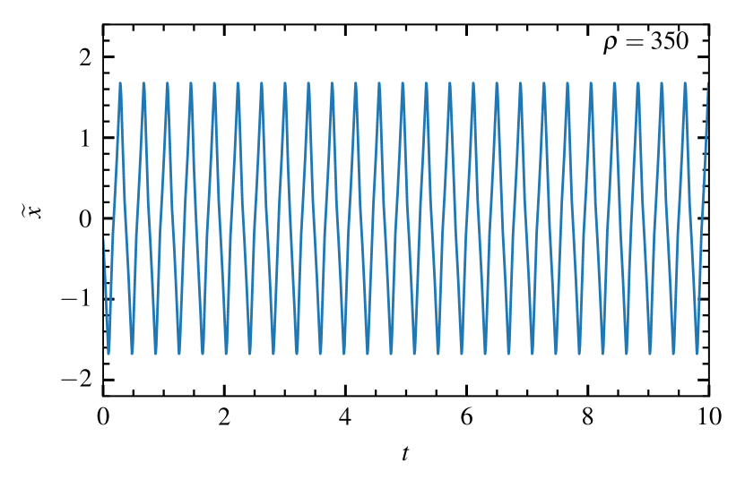
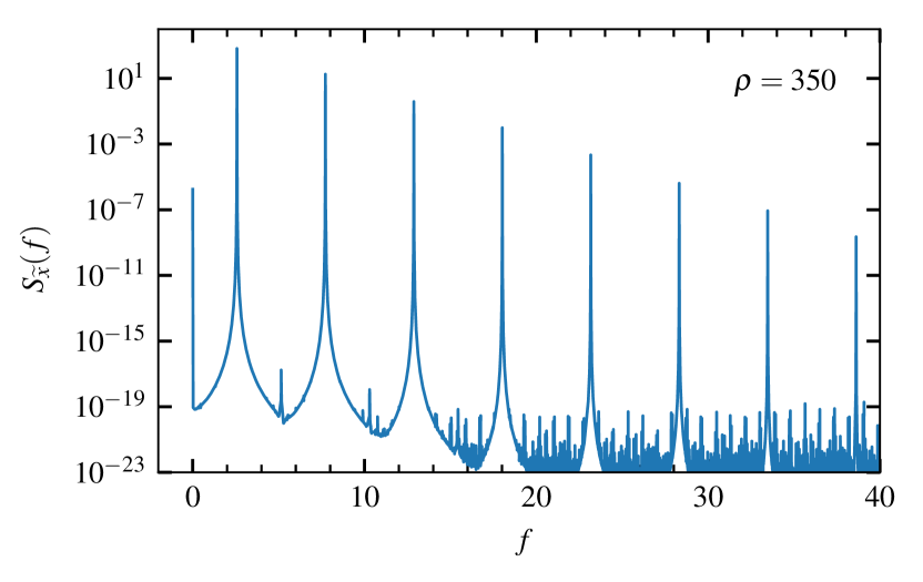
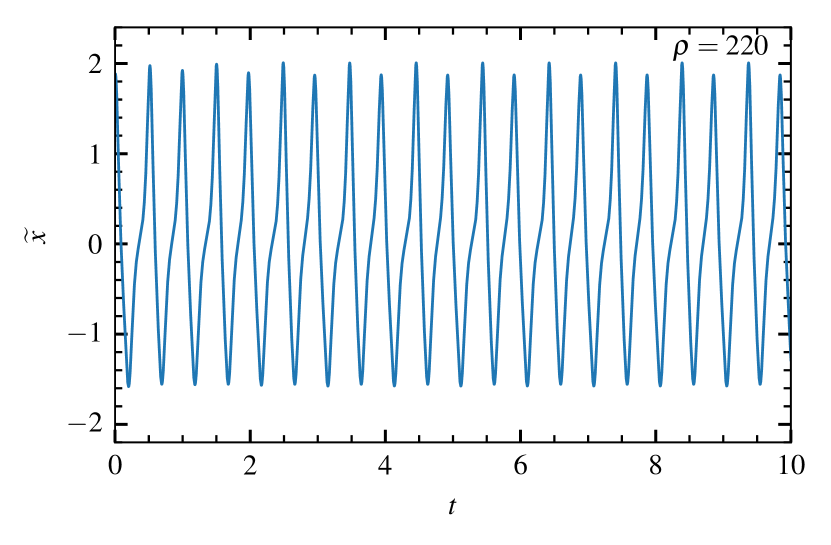
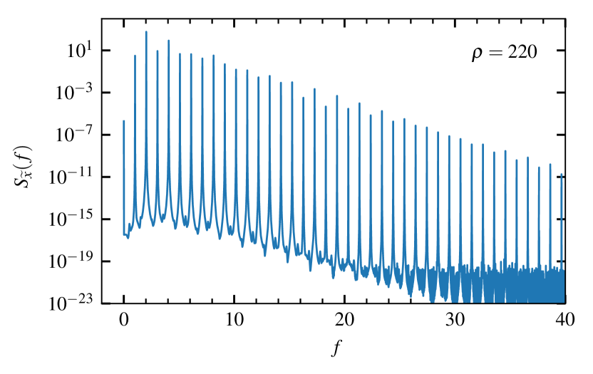
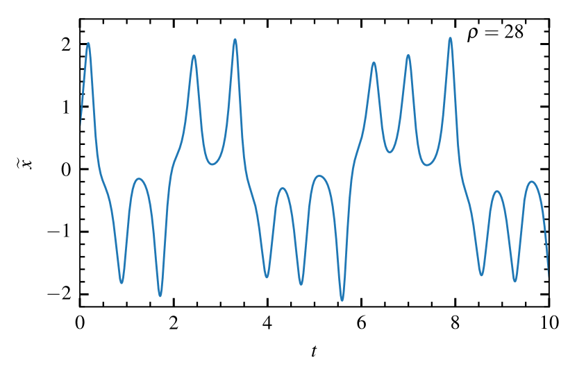
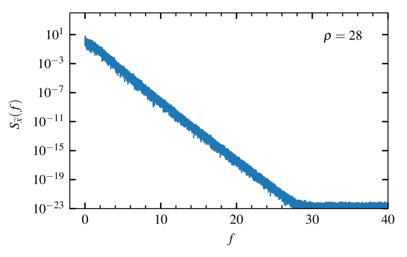
Figure 1: Excerpts of time series of the $\widetilde{x}$-variable of the Lorenz system (left) with corresponding power spectral densities (right) for $\sigma=10$, $\beta=8/3$ and three different values of the $\rho$ parameter.

Representative excerpts of the $x$-variable is presented in Fig. 1 for $\sigma=10$, $\beta=8/3$ and three different values of the model parameter $\rho$ together with their corresponding power spectral densities. The power spectra are presented with semi-logarithmic axes in order to readily identify exponential variation. For $\rho=350$ (top) the solution consists of nearly periodic oscillations and the frequency PSD resembles a Dirac comb with an exponential modulation of the peak amplitudes. The time between two consecutive positive peaks in the time series is $0.39$, while the peak separation in the PSD is $5.15$. The peak amplitudes in the PSD decay with a slope of $0.74$. Following a period-doubling bifurcation, the solution for $\rho=220$ (middle) is still regular and the PSD is again dominated by a Dirac-like comb with an exponential modulation. The distance between two positive peaks in the time series is $0.98$, while the peak separation in the PSD is $1.02$. The peak amplitudes in the PSD decay with a slope of $0.76$. For $\rho=28$ (bottom) the solution is chaotic and the PSD has an exponential shape with slope $1.9$ for all but the lowest frequencies. The flat spectral part at high frequencies is due to noise associated with round off errors in the computations. In the following, these features of the dynamics will be analyzed and connected by describing the fluctuations as a super-position of Lorentzian-shaped pulses.

III The power spectral density of a sum of pulses

In this section, we derive an expression for the PSD of a process consisting of randomly as well as periodically arriving, superposed pulses. This is based on the formalism developed for the FPP.[32, 33, 34, 48] We consider a train of $K(T)$ pulses arriving in the interval of duration $T$ with randomly distributed arrival times $\{t_{k}\}_{k=1}^{K(T)}$ and randomly distributed amplitudes $\{A_{k}\}_{k=1}^{K(T)}$. All pulses are assumed to have the same function form $\varphi$ and fixed duration $\tau_{\text{d}}$, so the process can be written as

$$\Phi_{K}(t)=\sum_{k=1}^{K(T)}A_{k}\varphi(\frac{t-t_{k}}{\tau_{\text{d}}}).$$ (5)

The number of pulses $K$ only depends on the duration $T$ of the time interval under consideration, not the value of the starting time. For convenience, we choose the interval to be $[-T/2,T/2]$. The number of pulses $K(T)$ is distributed according to the probability distribution $P_{K}(K;T,\tau_{\text{w}})$ depending on the duration $T$ and the average waiting time between arrivals $\tau_{\text{w}}$. For independent as well as identically and uniformly distributed pulse arrivals, $K(T)$ is Poisson distributed and the sorted waiting times are independent and exponentially distributed with mean value $\tau_{w}$. For periodic arrivals, $K(T)$ is approximately degenerately distributed with $\langle K\rangle=\mathopen{}\mathclose{{}\left\lfloor T/\tau_{\text{w}}}\right\rfloor$ where $\mathopen{}\mathclose{{}\left\lfloor\cdot}\right\rfloor$ denotes the floor function. In this case, the waiting times are degenerately distributed with mean value $\tau_{\text{w}}$. Further discussion of periodic pulse arrivals are given in App. C.

III.1 Separating pulses and forcing

Following the remarks in the introduction, the process is written as a convolution between a pulse train $F_{K}$ and a pulse function $\varphi$,

$$\Phi_{K}(t)=\int_{-\infty}^{\infty}\text{d}s\,\varphi\mathopen{}\mathclose{{}\left(\frac{t}{\tau_{\text{d}}}-s}\right)F_{K}(s),$$ (6)

where the forcing is

$$F_{K}(s)=\sum_{k=1}^{K(T)}A_{k}\delta\mathopen{}\mathclose{{}\left(s-\frac{t_{k}}{\tau_{\text{d}}}}\right),$$ (7)

and $\delta$ denotes the Dirac delta function. This can be viewed as a point process $F_{K}$ passed through a filter with response function $\varphi$, hence the name FPP.

We normalize the pulse function such that

$$\int_{-\infty}^{\infty}\text{d}s\,\lvert\varphi(s)\rvert=1.$$ (8)

We also introduce the notation

$$\rho_{\varphi}(s)=\frac{1}{I_{2}}\int\limits_{-\infty}^{\infty}\text{d}u\,\varphi(u)\varphi(u+s)$$ (9)

and

$$\varrho_{\varphi}(\theta)=\frac{1}{I_{2}}\lvert\mathcal{F}\mathopen{}\mathclose{{}\left[{\varphi}}\right](\theta)\rvert^{2}$$ (10)

for the auto-correlation and the PSD of the pulse function, respectively. Here, the pulse integral of order $n$ is defined by

$$I_{n}=\int_{-\infty}^{\infty}\text{d}s\,[\varphi(s)]^{n}.$$ (11)

Note that the functions $\rho_{\varphi}$ and $\varrho_{\varphi}$ form a Fourier transform pair, where the definition of the Fourier transform is given in App. B. We further note that $\rho_{\phi}(0)=1$ and $\varrho_{\phi}(0)=I_{1}^{2}/I_{2}$. Throughout this contribution, we will assume Lorentzian pulses, which are detailed in App. F. In particular, these have the auto-correlation

$$\rho_{\varphi}(s)=\frac{4}{4+s^{2}}$$ (12)

and power spectral density

$$\varrho_{\varphi}(\theta)=2\pi\exp(-2\lvert\theta\rvert).$$ (13)

To obtain the PSD, we start from Eq. (6), and take the finite-time Fourier transform as defined in App. B,

$$\mathcal{F}_{T}\mathopen{}\mathclose{{}\left[{\Phi_{K}}}\right](\omega)=\int\limits_{-T/2}^{T/2}\text{d}t\,\exp(-i\omega t)\Phi_{K}(t)=\int\limits_{-T/2}^{T/2}\text{d}t\,\exp(-i\omega t)\int\limits_{-\infty}^{\infty}\text{d}s\,\varphi(s)F_{K}\mathopen{}\mathclose{{}\left(\frac{t}{\tau_{\text{d}}}-s}\right),$$ (14)

where we have exchanged the functions in the convolution given by Eq. (6). A change of variables defined by $u(t)=t-\tau_{\text{d}}s$ gives

$$\mathcal{F}_{T}\mathopen{}\mathclose{{}\left[{\Phi_{K}}}\right](\omega)=\int\limits_{-\infty}^{\infty}\text{d}s\,\varphi(s)\exp(-i\tau_{\text{d}}\omega s)\int\limits_{-T/2-\tau_{\text{d}}s}^{T/2-\tau_{\text{d}}s}\text{d}u\,F_{K}\mathopen{}\mathclose{{}\left(\frac{u}{\tau_{\text{d}}}}\right)\exp(-i\omega u).$$ (15)

We assume that $\varphi(s)$ is negligible after a few $\tau_{\text{d}}$. Assuming $T/\tau_{\text{d}}\gg 1$, we can therefore approximate the limits of the second integral in Eq. (15) as $u\in\mathopen{}\mathclose{{}\left[-T/2,T/2}\right]$, and the two integrals become independent. This gives

$$\mathcal{F}_{T}\mathopen{}\mathclose{{}\left[{\Phi_{K}}}\right](\omega)=\mathcal{F}\mathopen{}\mathclose{{}\left[{\varphi}}\right](\tau_{\text{d}}\omega)\mathcal{F}_{T}\mathopen{}\mathclose{{}\left[{F_{K}}}\right](\omega).$$ (16)

The PSD of the stationary process $\Phi$ is therefore

$$\mathcal{S}_{\Phi}(\omega)=\lim_{T\to\infty}\frac{1}{T}\mathopen{}\mathclose{{}\left<\lvert\mathcal{F}_{T}\mathopen{}\mathclose{{}\left[{\Phi_{K}}}\right](\omega)\rvert^{2}}\right>=\lvert\mathcal{F}\mathopen{}\mathclose{{}\left[{\varphi}}\right](\tau_{\text{d}}\omega)\rvert^{2}\lim_{T\to\infty}\frac{1}{T}\mathopen{}\mathclose{{}\left<\lvert\mathcal{F}_{T}\mathopen{}\mathclose{{}\left[{F_{K}}}\right](\omega)\rvert^{2}}\right>,$$ (17)

where $\mathcal{S}_{\Phi}(\omega)$ is independent of $K$, since the average is over all random variables. The power spectrum is thus the product of the power spectrum of the pulse function and the power spectrum of the point process. The arrival time distribution only affects the point process, so this will be isolated in the analysis in Sec. III.2.

Using Eq. (10), the full PSD of $\Phi$ can be written as

$$\mathcal{S}_{\Phi}(\omega)=I_{2}\varrho_{\varphi}(\tau_{\text{d}}\omega)\lim_{T\to\infty}\frac{1}{T}\mathopen{}\mathclose{{}\left<\lvert\mathcal{F}_{T}\mathopen{}\mathclose{{}\left[{F_{K}}}\right](\omega)^{2}\rvert}\right>.$$ (18)

Thus, the PSD is given by the spectrum of the forcing modulated by that of the pulse function.

For reference, we note that for Poisson distributed $K(T)$ and amplitudes independent of the pulse arrivals, the PSD of $\Phi$ may be written as [28, 49]

$$\mathcal{S}_{\Phi}(\omega)=2\pi\langle\Phi\rangle^{2}\delta(\omega)+\tau_{\text{d}}\Phi_{\text{rms}}^{2}\varrho_{\phi}\mathopen{}\mathclose{{}\left(\tau_{\text{d}}\omega}\right).$$ (19)

Here, $\langle\Phi\rangle=\gamma\mathopen{}\mathclose{{}\left<A}\right>I_{1}$ and $\Phi_{\text{rms}}^{2}=\gamma\langle A^{2}\rangle I_{2}$ are the mean value and the variance of $\Phi$, respectively.

III.2 General arrival times

The Fourier transform of the point process is

$$\mathcal{F}_{T}\mathopen{}\mathclose{{}\left[{F_{K}}}\right](\omega)=\tau_{\text{d}}\sum_{k=1}^{K}A_{k}\exp(-i\omega t_{k}).$$ (20)

Multiplying this expression with its complex conjugate and averaging over all random variables gives

$$\frac{1}{T}\mathopen{}\mathclose{{}\left<\lvert\mathcal{F}_{T}\mathopen{}\mathclose{{}\left[{F_{K}}}\right](\omega)^{2}\rvert}\right>=\sum_{K=0}^{\infty}P_{K}(K;T,\tau_{\text{w}})\frac{\tau_{\text{d}}^{2}}{T}\sum_{k,l=1}^{K}\mathopen{}\mathclose{{}\left<A_{k}A_{l}}\right>\mathopen{}\mathclose{{}\left<\exp\mathopen{}\mathclose{{}\left(i\omega(t_{l}-t_{k}}\right))}\right>.$$ (21)

Here we have assumed that the pulse amplitudes are independent of the arrival times. In the following, we will further assume that the amplitudes are pairwise uncorrelated and identically distributed so that $\langle A_{k}A_{l}\rangle=(\langle A^{2}\rangle-\langle A\rangle^{2})\delta_{kl}+\langle A^{2}\rangle$. In the double sum in Eq. (21) there are $K$ terms for which $k=l$ and $K(K-1)$ terms for which $k\neq l$. Summing over all these terms, we have

$$\frac{1}{T}\mathopen{}\mathclose{{}\left<\lvert\mathcal{F}_{T}\mathopen{}\mathclose{{}\left[{F_{K}}}\right](\omega)^{2}\rvert}\right>=\\ \tau_{\text{d}}^{2}\sum_{K=0}^{\infty}P_{K}(K;T,\tau_{\text{w}})\mathopen{}\mathclose{{}\left\{\frac{K}{T}\langle{A^{2}}\rangle+\frac{1}{T}\mathopen{}\mathclose{{}\left<A}\right>^{2}\sum_{k=1}^{K}\sum_{l\neq k}\mathopen{}\mathclose{{}\left<\exp\mathopen{}\mathclose{{}\left(i\omega(t_{l}-t_{k}}\right))}\right>}\right\}.$$ (22)

The sum of averaged exponential functions is the joint characteristic function of $t_{l}$ and $t_{k}$. Exchanging the order of $k$ and $l$ in the double sum is the same as taking the complex conjugate of this characteristic function, so we get

$$\frac{1}{T}\mathopen{}\mathclose{{}\left<\lvert\mathcal{F}_{T}\mathopen{}\mathclose{{}\left[{F_{K}}}\right](\omega)^{2}\rvert}\right>=\frac{\tau_{\text{d}}^{2}\langle K\rangle}{T}\langle{A^{2}}\rangle+\\ \frac{\tau_{\text{d}}^{2}}{T}\mathopen{}\mathclose{{}\left<A}\right>^{2}\sum_{K=0}^{\infty}P_{K}(K;T,\tau_{\text{w}})\sum_{k=2}^{K}\sum_{l=1}^{k-1}2\text{Re}\mathopen{}\mathclose{{}\left[\mathopen{}\mathclose{{}\left<\exp\mathopen{}\mathclose{{}\left(i\omega(t_{l}-t_{k}}\right))}\right>}\right],$$ (23)

where the operator $\text{Re}[\cdot]$ denotes the real part of the argument. Thus the PSD is real, as required.

III.2.1 Independent and uniformly distributed arrivals

As an example, we show that the expression in Eq. (23) is consistent with the established result for $K(T)$ a stationary Poisson point process. In this case $t_{l}$ and $t_{k}$ are independent and uniformly distributed arrivals on the interval $[0,T]$. We therefore have that

$$\mathopen{}\mathclose{{}\left<\exp\mathopen{}\mathclose{{}\left(i\omega(t_{l}-t_{k}}\right))}\right>=\mathopen{}\mathclose{{}\left<\exp\mathopen{}\mathclose{{}\left(i\omega t_{l}}\right)}\right>\mathopen{}\mathclose{{}\left<\exp\mathopen{}\mathclose{{}\left(-i\omega t_{k}}\right)}\right>=2\,\frac{1-\cos(\omega T)}{\omega^{2}T^{2}}.$$ (24)

All terms in the double sum in Eq. (23) are equal, and we get

$$\frac{1}{T}\mathopen{}\mathclose{{}\left<\lvert\mathcal{F}_{T}\mathopen{}\mathclose{{}\left[{F_{K}}}\right](\omega)^{2}\rvert}\right>=\frac{\tau_{\text{d}}^{2}\langle K\rangle}{T}\langle{A^{2}}\rangle+\frac{2\tau_{\text{d}}^{2}}{T}\mathopen{}\mathclose{{}\left<A}\right>^{2}\mathopen{}\mathclose{{}\left<K(K-1)}\right>\frac{1-\cos(\omega T)}{\omega^{2}T^{2}}.$$ (25)

Since $K$ is Poisson distributed with mean and variance both equal to $T/\tau_{\text{w}}$ we get

$$\frac{1}{T}\mathopen{}\mathclose{{}\left<\lvert\mathcal{F}_{T}\mathopen{}\mathclose{{}\left[{F_{K}}}\right](\omega)^{2}\rvert}\right>=\frac{\tau_{\text{d}}^{2}}{\tau_{\text{w}}}\langle{A^{2}}\rangle+\frac{2\tau_{\text{d}}^{2}}{\tau_{\text{w}}^{2}}\mathopen{}\mathclose{{}\left<A}\right>^{2}T\frac{1-\cos(\omega T)}{\omega^{2}T^{2}},$$ (26)

which gives, using $\gamma=\tau_{\text{d}}/\tau_{\text{w}}$ and that the last term contains the function $f_{T}(\omega)$ defined in App. G,

$$\lim_{T\to\infty}\frac{1}{T}\mathopen{}\mathclose{{}\left<\lvert\mathcal{F}_{T}\mathopen{}\mathclose{{}\left[{F_{K}}}\right](\omega)^{2}\rvert}\right>=\tau_{\text{d}}\gamma\langle{A^{2}}\rangle+2\pi\tau_{\text{d}}\gamma^{2}\mathopen{}\mathclose{{}\left<A}\right>^{2}\delta(\tau_{\text{d}}\omega).$$ (27)

Multiplying this expression by the spectrum of the pulse function gives the standard expression for the PSD of the FPP,[49, 50]

$$\mathcal{S}_{\Phi}(\omega)=\tau_{\text{d}}\gamma\langle{A^{2}}\rangle I_{2}\varrho_{\varphi}(\tau_{\text{d}}\omega)+2\pi\tau_{\text{d}}\gamma^{2}\mathopen{}\mathclose{{}\left<A}\right>^{2}I_{1}^{2}\delta(\tau_{\text{d}}\omega).$$ (28)

A Poisson point process gives a flat spectrum, so the only frequency variation for the filtered process is due to the pulse function.

III.2.2 Periodic arrival times

We consider the situation where the periodicity is known, but the exact arrivals are not. This corresponds to uncertainty in where the measurement starts in relation to the first arrival time. If the arrivals are strictly periodic, the marginal PDF of arrival $k$, given the starting time $r$, is

$$P_{t_{k}|r}\mathopen{}\mathclose{{}\left(t_{k}|r}\right)=\delta\mathopen{}\mathclose{{}\left(t_{k}-\tau_{\text{p}}k-r}\right).$$ (29)

Since each arrival is deterministic, the joint PDF with known starting point is the product of the marginal PDFs, and we have

$$\mathopen{}\mathclose{{}\left<\exp\mathopen{}\mathclose{{}\left(i\omega(t_{l}-t_{k}}\right))}\right>=\exp(i\omega\tau_{\text{p}}(l-k)).$$ (30)

Note that this is independent of the starting time $r$, so for now we need not consider $r$ further. We then have from Eq. (23)

$$\sum_{k=2}^{K}\sum_{l=1}^{k-1}2\text{Re}\mathopen{}\mathclose{{}\left[\mathopen{}\mathclose{{}\left<\exp\mathopen{}\mathclose{{}\left(i\omega(t_{l}-t_{k}}\right))}\right>}\right]=\sum_{k=2}^{K}\sum_{l=1}^{k-1}2\cos\mathopen{}\mathclose{{}\left(\tau_{\text{p}}\omega(l-k)}\right)=\frac{\cos\mathopen{}\mathclose{{}\left(\tau_{\text{p}}\omega K}\right)-1}{\cos\mathopen{}\mathclose{{}\left(\tau_{\text{p}}\omega}\right)-1}-K.$$ (31)

Inserting Eq. (31) into Eq. (23) gives

$$\frac{1}{T}\mathopen{}\mathclose{{}\left<\lvert\mathcal{F}_{T}\mathopen{}\mathclose{{}\left[{F_{K}}}\right](\omega)^{2}\rvert}\right>=\tau_{\text{d}}^{2}A_{\text{rms}}^{2}\frac{\langle K\rangle}{T}+\tau_{\text{d}}^{2}\mathopen{}\mathclose{{}\left<A}\right>^{2}\frac{1}{T}\frac{\langle\cos\mathopen{}\mathclose{{}\left(\tau_{\text{p}}\omega K}\right)\rangle-1}{\cos\mathopen{}\mathclose{{}\left(\tau_{\text{p}}\omega}\right)-1}.$$ (32)

Due to the periodicity, there are either $\mathopen{}\mathclose{{}\left\lfloor T/\tau_{\text{p}}}\right\rfloor-1$ or $\mathopen{}\mathclose{{}\left\lfloor T/\tau_{\text{p}}}\right\rfloor$ events in a time series of length $T$, see App. C for details. Thus, for $T/\tau_{\text{p}}\gg 1$, we make the approximation $K=\mathopen{}\mathclose{{}\left\lfloor T/\tau_{\text{p}}}\right\rfloor$ and have

$$\lim_{T\to\infty}\frac{1}{T}\mathopen{}\mathclose{{}\left<\lvert\mathcal{F}_{T}\mathopen{}\mathclose{{}\left[{F_{K}}}\right](\omega)^{2}\rvert}\right>=\frac{\tau_{\text{d}}^{2}}{\tau_{\text{p}}}A_{\text{rms}}^{2}+\frac{\tau_{\text{d}}^{2}}{\tau_{\text{p}}}\mathopen{}\mathclose{{}\left<A}\right>^{2}\lim_{K\to\infty}\frac{\cos\mathopen{}\mathclose{{}\left(\tau_{\text{p}}\omega K}\right)-1}{K\mathopen{}\mathclose{{}\left[\cos\mathopen{}\mathclose{{}\left(\tau_{\text{p}}\omega}\right)-1}\right]}.$$ (33)

Let us consider the limit in the last term on the right hand side,

$$\lim_{K\to\infty}\frac{1}{K}\frac{\cos\mathopen{}\mathclose{{}\left(\tau_{\text{p}}\omega K}\right)-1}{\cos\mathopen{}\mathclose{{}\left(\tau_{\text{p}}\omega}\right)-1}.$$ (34)

For integer $n$ and $\tau_{\text{p}}\omega\neq 2\pi n$, this limit is zero. However, for $\tau_{\text{p}}\omega\to 2\pi n$, this limit tends to infinity. We might therefore consider Eq. (34) proportional to a train of $\delta$-pulses located at $\tau_{\text{p}}\omega=2\pi n$. Setting $\tau_{\text{p}}\omega=2\pi n+\epsilon$ where $\epsilon\ll 1$ and expanding the cosine in the denominator, we have

$$\lim_{K\to\infty}\frac{1}{K}\frac{\cos\mathopen{}\mathclose{{}\left(\tau_{\text{p}}\omega K}\right)-1}{\cos\mathopen{}\mathclose{{}\left(\tau_{\text{p}}\omega}\right)-1}=\lim_{K\to\infty}\frac{2}{K}\frac{1-\cos\mathopen{}\mathclose{{}\left(\epsilon K}\right)}{\epsilon^{2}}.$$ (35)

This is on the same form as we had when deriving Eq. (27), so we conclude that

$$\lim_{K\to\infty}\frac{1}{K}\frac{\cos\mathopen{}\mathclose{{}\left(\tau_{\text{p}}\omega K}\right)-1}{\cos\mathopen{}\mathclose{{}\left(\tau_{\text{p}}\omega}\right)-1}=2\pi\sum\limits_{n=-\infty}^{\infty}\delta\mathopen{}\mathclose{{}\left(\tau_{\text{p}}\omega-2\pi n}\right).$$ (36)

Inserting this into Eq. (32) gives the full expression for the PSD of a periodic train of delta pulses with randomly distributed amplitudes,

$$\lim_{T\to\infty}\frac{1}{T}\mathopen{}\mathclose{{}\left<\lvert\mathcal{F}_{T}\mathopen{}\mathclose{{}\left[{F_{K}}}\right](\omega)^{2}\rvert}\right>=\tau_{\text{d}}\gamma A_{\text{rms}}^{2}+2\pi\tau_{\text{d}}\gamma^{2}\mathopen{}\mathclose{{}\left<A}\right>^{2}\sum\limits_{n=-\infty}^{\infty}\delta\mathopen{}\mathclose{{}\left(\tau_{\text{d}}\omega-2\pi n\gamma}\right).$$ (37)

where $\gamma=\tau_{\text{d}}/\tau_{\text{p}}$. This equation will be discussed in the following section. We note that this result is also obtained by using the full distribution of $K$ from App. C.

IV Periodic pulse arrivals

In this section we derive the PSD and auto-correlation function in the case of periodic pulse arrivals and discuss the role of finite mean value and standard deviation of the pulse amplitudes.

IV.1 The power spectral density

The frequency PSD of $\Phi$ is given by multiplying Eq. (37) with the power spectrum of the pulse function, Eq. (10), as given by Eq. (18),

$$\mathcal{S}_{\Phi}(\omega)=\tau_{\text{d}}\gamma A_{\text{rms}}^{2}I_{2}\varrho_{\varphi}(\tau_{\text{d}}\omega)+2\pi\tau_{\text{d}}\gamma^{2}\mathopen{}\mathclose{{}\left<A}\right>^{2}I_{2}\varrho_{\varphi}(\tau_{\text{d}}\omega)\sum\limits_{n=-\infty}^{\infty}\delta\mathopen{}\mathclose{{}\left(\tau_{\text{d}}\omega-2\pi n\gamma}\right).$$ (38)

There are two main differences from the case with Poisson arrivals, given by Eq. (27): Firstly, $A_{\text{rms}}$ enters into the first term instead of $\langle{A^{2}}\rangle$. Secondly, there is a contribution of delta spikes at integer multiples of $2\pi/\tau_{\text{p}}$ with an envelope or modulation given by the spectrum of the pulse function. We may view the first term as the average spectrum, due to the randomness of the amplitudes, while the second term containing the sum of delta functions is due to the periodicity of the pulse arrivals. Accordingly, the first term vanishes for degenerately distributed amplitudes, $p_{A}(A)=\delta(A-\mathopen{}\mathclose{{}\left<A}\right>)$. For a symmetric amplitude distribution with vanishing mean, $\mathopen{}\mathclose{{}\left<A}\right>=0$ and $A_{\text{rms}}^{2}=\langle{A^{2}}\rangle$, the periodicity cancels out and only the first term remains.

In Fig. 2 the empirical PSD (left) and auto-correlation function (right, to be discussed in the following) for realizations of the process is presented for exponentially distributed amplitudes (blue line) and for symmetrically Laplace distributed amplitudes with vanishing mean (orange line). In both cases the arrivals are periodic and the pulses have a symmetric Lorentzian shape as defined in App. F. The analytical expression given by Eq. (38) for the two cases is presented by the black and green dashed lines, respectively. The Dirac comb with decaying peak amplitudes is clearly seen in the case with exponentially distributed amplitudes. We emphasize that the main effect of the periodicity, the Dirac comb, is completely cancelled out in the case of symmetrically distributed pulse amplitudes with vanishing mean.

On the left-hand side of Fig. 3, we show that the Dirac comb is not discontinuously lost when we go from $\mathopen{}\mathclose{{}\left<A}\right>\neq 0$ to $\mathopen{}\mathclose{{}\left<A}\right>=0$, but it decays as the value of $\mathopen{}\mathclose{{}\left<A}\right>$ goes to zero. Here, we use asymmetrically Laplace distributed amplitudes with asymmetry parameter $\lambda$, see App. I.2. The exponential amplitude distribution is recovered for $\lambda=0$, while the symmetric Laplace distribution is given by $\lambda=1/2$. As $\lambda$ goes from $0$ to $1/2$, the mass of the Dirac comb gradually decays. The same effect is seen in the auto-correlation function, shown on the right-hand side of Fig. 3.

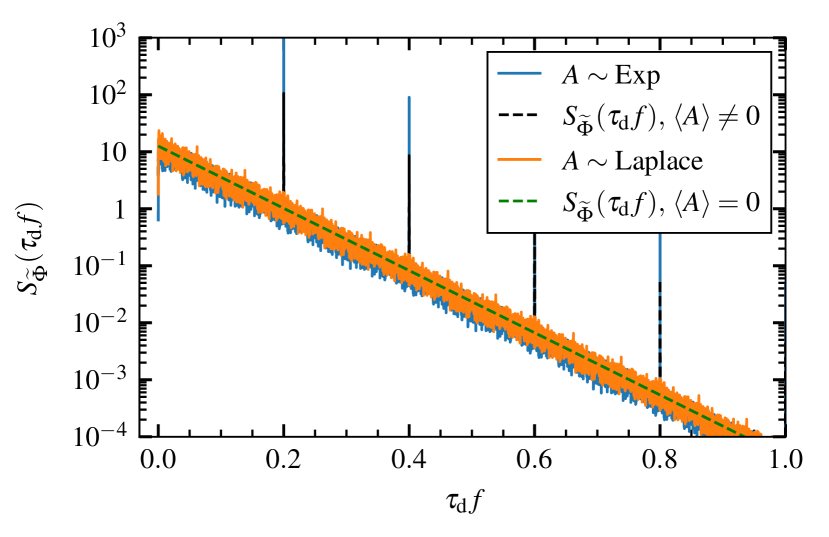
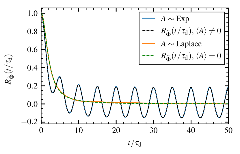
Figure 2: Power spectral density (left) and auto-correlation function (right) for a sum of Lorentzian pulses with periodic arrival times and exponential (blue) and Laplace (orange) distributed amplitudes. The analytical expressions are given by the black and green dashed lines, respectively.

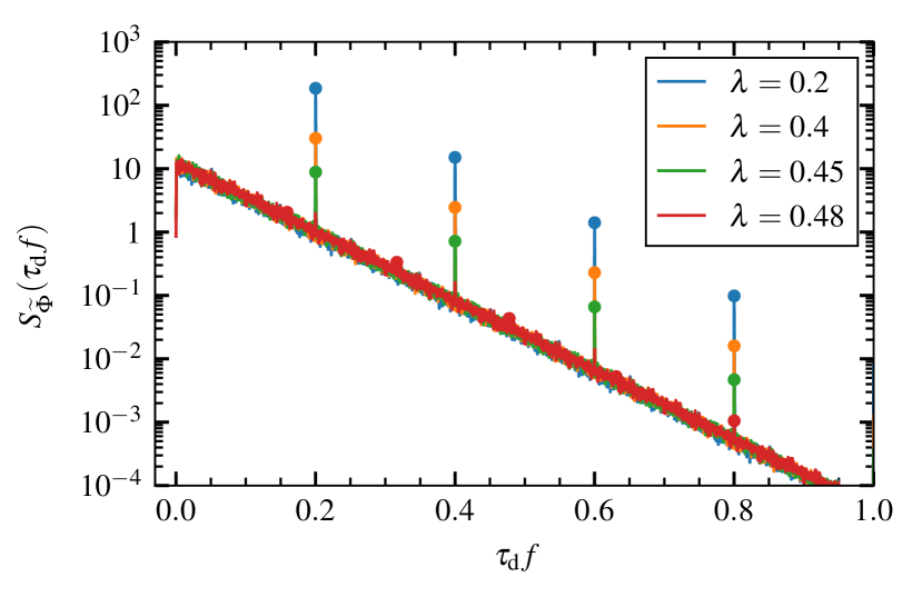
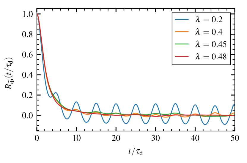
Figure 3: Power spectral density (left) and auto-correlation function (right) for a sum of Lorentzian pulses with periodic arrival times and Laplace distributed amplitudes with various asymmetry parameters $\lambda$ in the case $\tau_{\text{p}}=5\tau_{\text{d}}$. The filled circles indicate the mass of the delta functions.

IV.2 The auto-correlation function

By the Wiener-Khinchin theorem, the auto-correlation function $R_{\Phi}(t)$ is given by the inverse Fourier transform of the PSD,

$$R_{\Phi}(t) =\frac{1}{2\pi}\int\limits_{-\infty}^{\infty}\text{d}\omega\,\mathcal{S}_{\Phi}(\omega)\exp(i\omega t)$$ (39)

$$=\gamma A_{\text{rms}}^{2}I_{2}\rho_{\varphi}(t/\tau_{\text{d}})+\gamma^{2}\mathopen{}\mathclose{{}\left<A}\right>^{2}I_{2}\sum_{n=-\infty}^{\infty}\varrho_{\varphi}(2\pi n\gamma)\exp(i2\pi n\gamma t/\tau_{\text{d}}).$$ (40)

Using the Poisson summation formula and properties of the Fourier transform as detailed in App. E, we can write the auto-correlation function as

$$R_{\Phi}(t)=\gamma A_{\text{rms}}^{2}I_{2}\rho_{\varphi}\mathopen{}\mathclose{{}\left(\frac{t}{\tau_{\text{d}}}}\right)+\gamma\mathopen{}\mathclose{{}\left<A}\right>^{2}I_{2}\sum_{m=-\infty}^{\infty}\rho_{\varphi}\mathopen{}\mathclose{{}\left(\frac{m}{\gamma}+\frac{t}{\tau_{\text{d}}}}\right).$$ (41)

Writing $m/\gamma+t/\tau_{\text{d}}=(m+t/\tau_{\text{p}})/\gamma$, we see that the correlation function consists of a central peak followed by periodic oscillations with peaks at integer multiples of $\tau_{\text{p}}$. For a degenerate distribution of pulse amplitudes the correlation function only consists of the periodic train: there is no randomness left in the signal and so the correlation function does not decay for large times. For a symmetric distribution of the amplitudes with vanishing mean, only the central peak remains and the auto-correlation function for the process is given by that of the pulse function.

On the right-hand side of Fig. 2, the auto-correlation function of a synthetically generated time series is presented for exponentially distributed amplitudes (blue line) and symmetrical Laplace distributed amplitudes (orange line). The arrivals are periodic and the pulses have a Lorentzian shape. The analytic expression given by Eq. (38) is presented by the black and green dashed lines for the corresponding cases, respectively. For exponentially distributed amplitudes, the periodicity is clearly seen. This effect is again completely cancelled out in the case of a symmetric distribution of pulse amplitudes with vanishing mean.

IV.3 The mean value and standard deviation

The mean value of the process $\Phi$ for the conditional case of exactly $K$ events with periodic pulse arrivals is given by

$$\mathopen{}\mathclose{{}\left<\Phi_{K}}\right> =\sum_{k=1}^{K(T)}\int_{-\infty}^{\infty}\text{d}A\,P_{A}(A)\int_{0}^{\tau_{\text{p}}}\text{d}r\,P_{r}(r)A\varphi\mathopen{}\mathclose{{}\left(\frac{t-\tau_{\text{p}}k-r}{\tau_{\text{d}}}}\right)$$

$$=\frac{\mathopen{}\mathclose{{}\left<A}\right>}{\tau_{\text{p}}}\sum_{k=1}^{K(T)}\int\limits_{0}^{\tau_{\text{p}}}\text{d}r\,\varphi\mathopen{}\mathclose{{}\left(\frac{t-\tau_{\text{p}}k-r}{\tau_{\text{d}}}}\right)$$ (42)

Averaging over the number of pulses gives the mean value for the stationary process

$$\mathopen{}\mathclose{{}\left<\Phi}\right>=\lim_{T\to\infty}\sum_{K=1}^{\infty}P_{K}(K;T,\tau_{\text{w}})\mathopen{}\mathclose{{}\left<\Phi_{K}}\right>=\gamma\mathopen{}\mathclose{{}\left<A}\right>I_{1}.$$ (43)

In the last step, we let $T\to\infty$ giving $K\to\infty$ and set the upper integration limit to infinity to avoid the effect due to the signal starting at $t=0$. This is the expected result from Campbell’s theorem. [51, 52] This is also consistent with the fact that the square of the mean value is given by the zero-frequency delta function in the power spectrum as given by Eq. (38).

The second order moment is most conveniently found by noting that the variance is

$$\mathopen{}\mathclose{{}\left<\Phi^{2}}\right>=R_{\Phi}(0)=\gamma A_{\text{rms}}^{2}I_{2}+\gamma\mathopen{}\mathclose{{}\left<A}\right>^{2}I_{2}\sum\limits_{m=-\infty}^{\infty}\rho_{\varphi}\mathopen{}\mathclose{{}\left(\frac{m}{\gamma}}\right),$$ (44)

where we have used that $\rho_{\varphi}(0)=1$. This can be verified by calculating the second order moment directly as was done for the mean above. In App. D, it is shown that this is also equivalent to an extension of Campbell’s theorem. We thus get the variance

$$\Phi_{\text{rms}}^{2}=\gamma A_{\text{rms}}^{2}I_{2}+\gamma\mathopen{}\mathclose{{}\left<A}\right>^{2}I_{2}\mathopen{}\mathclose{{}\left(\sum_{m=-\infty}^{\infty}\rho_{\varphi}(m/\gamma)-\gamma\frac{I_{1}^{2}}{I_{2}}}\right).$$ (45)

In the case $\gamma\ll 1$, only the $m=0$ term in the sum gives a contribution, $\rho_{\varphi}(0)=1$, giving

$$\lim\limits_{\gamma\to 0}\frac{1}{\gamma}\,\Phi_{\text{rms}}^{2}=\langle{A^{2}}\rangle I_{2},$$ (46)

where we neglect the $\gamma^{2}$-contribution of the last term in the bracket in Eq. (45). Thus, in the limit of no pulse overlap, the variance for the case of periodic pulses is equivalent to the case of Poisson arrivals, discussed in Sec. III.2.1.

In the limit $\gamma\rightarrow\infty$, we can write $m/\gamma=m\,\text{d}s\to s$ and treat the sum as an integral, $(1/\gamma)\sum_{m}\rho_{\varphi}(m/\gamma)\to\int\rho_{\varphi}(s)\text{d}s=I_{1}^{2}/I_{2}$, where the sum is over all integers and the integral is over all reals. The terms inside the bracket in Eq. (45) cancel, and we get

$$\lim\limits_{\gamma\to\infty}\frac{1}{\gamma}\,\Phi_{\text{rms}}^{2}=A_{\text{rms}}^{2}I_{2}.$$ (47)

Since $A_{\text{rms}}^{2}=\langle{A^{2}}\rangle-\mathopen{}\mathclose{{}\left<A}\right>^{2}\leq\langle{A^{2}}\rangle$, the periodic pulse overlap gives lower variance than the case of Poisson arrivals as there is less randomness in the process. For an exponential amplitude distribution, the variance in the periodic case is a factor two smaller. For amplitudes with zero mean value, it is equal to the Poisson case. For fixed amplitudes, the process has no variance as pulses will accumulate until the rate of accumulation exactly matches the rate of decay, after which the signal will remain constant.

V Deviations from periodicity

In this section, we will consider deviations from strict periodicity in a few different ways. It will be demonstrated that the Dirac comb is a very robust feature of the model as long as periodic arrivals are maintained. However, slight deviations from periodic arrivals efficiently remove most higher harmonics in the Dirac comb.

V.1 Quasi-periodic pulses

In this section, we present the effect of quasi-periodicity in the arrival time distribution on the second-order statistics of the stochastic process. Here, we model quasi-periodicity using a uniform distribution for each arrival around the periodic arrival time, so that the distribution of the $k$’th arrival time given the starting time $r$ is

$$P_{t_{k}}\mathopen{}\mathclose{{}\left(t_{k}|r}\right)=\begin{cases}\displaystyle\frac{1}{2\tau_{\text{p}}\kappa},&-\tau_{\text{p}}\kappa\leq t_{k}-\tau_{\text{p}}k-r\leq\tau_{\text{p}}\kappa,\\ 0,&\text{else}.\end{cases}$$ (48)

In the limit $\kappa\to 0$, we recover the case of periodic arrivals, while for $\kappa>1$, the probability distributions of adjacent arrivals overlap. We emphasize that this is still a very restrictive formulation: even for $\kappa>1$, each arrival is guaranteed to be centered on the time corresponding to the periodic arrival time, and the number of arrivals in a given interval is fixed up to end effects.

In Fig. 4, an example of the effect of this quasi-periodicity is presented. The full lines give the power spectral densities and the auto-correlation functions of the process with quasi-periodic arrival times for different values of the $\kappa$-parameter, Lorentzian pulses and exponentially distributed amplitudes. The black dashed line gives the analytic prediction for strictly periodic pulses. Even moderate deviations from strict periodicity quickly destroy the Dirac comb. For $\kappa=1$, the spectrum and correlation function are already difficult to distinguish from the case of Poisson arrivals.

A similar result is seen in Figs. 5, where we have used Gamma distributed waiting times with scale parameter $\alpha$, shape parameter $\beta$ and constant mean value $\tau_{\text{p}}=\alpha\beta$. See App. I.1 for details. Everything else is equal to the previous case. For $\beta=1$, the waiting times would be exponentially distributed and only the modulation due to the pulse function would be present. For $\beta>1$, the waiting time distribution is unimodal with an exponential tail towards large waiting times. In the limit $\beta\to\infty$, the waiting time distribution approaches a Dirac delta function giving periodic arrivals. In the figures, it is evident that a very high shape parameter must be reached (that is, a very clear quasi-periodicity must be present in the signal) for the spectrum to display even a few harmonics. It is difficult to distinguish even $\beta=10$ from the case of Poisson arrivals.

These examples show that quasi-periodic phenomena in for example turbulent fluids cannot be expected to produce more than the first peak of the Dirac comb in the PSD, and that chaotic dynamics do not need to deviate far from strict periodicity in order for the Dirac comb to disappear. We will in Sec. VI see an example of this behavior for the chaotic case of the Lorenz system. We further note that in practice, this effect may hinder attempts at estimating the spectral decay from periodic peaks in the PSD of a measurement signal — a very strict periodicity is required to get a good estimate.

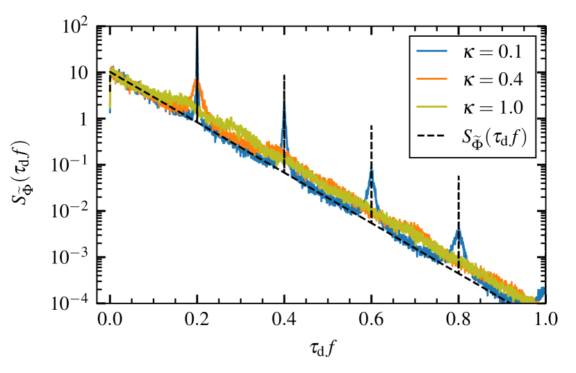
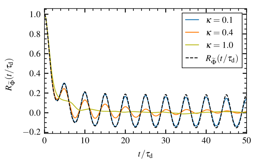
Figure 4: Power spectral density (left) and auto-correlation function (right) for a sum of Lorentzian pulses with quasi-periodic arrival times and various values of the $\kappa$-parameter. The analytical expression for strictly periodic pulses is presented by the black dashed line.

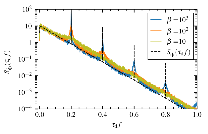
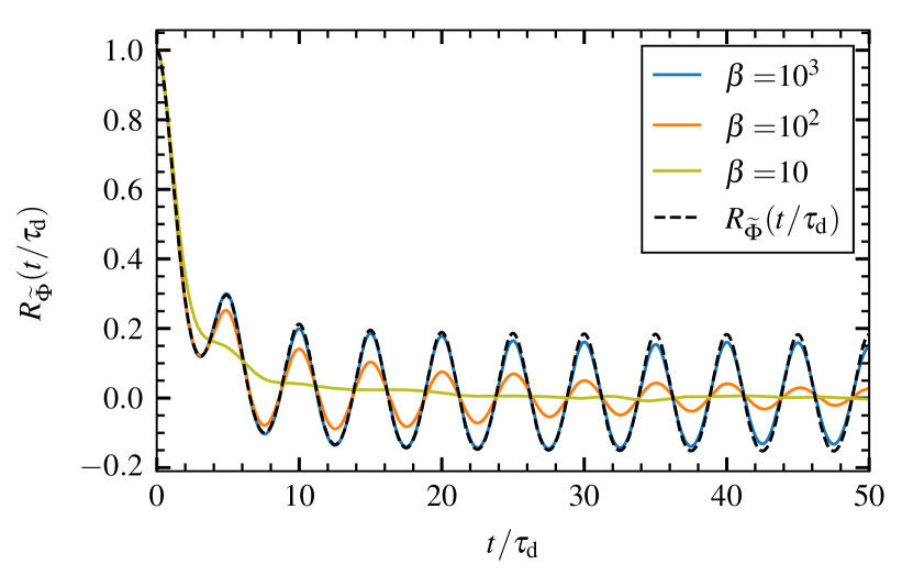
Figure 5: Power spectral density (left) and auto-correlation function (right) for realizations of the process with Gamma distributed waiting times and various values of the shape parameter $\beta$. The analytical expression for purely periodic pulses is presented by the black dashed line.

V.2 Multiple periodicities

In order to model period doubling, we now consider a situation where we have multiple periodicities, each with their own amplitudes and possible constant offsets. We then write the Fourier transform of the point process as

$$\mathcal{F}_{T}\mathopen{}\mathclose{{}\left[{F_{K}}}\right](\omega)=\tau_{\text{d}}\sum\limits_{p=1}^{\Pi}\sum\limits_{k=1}^{{}_{p}{K}}{}_{p}{A}_{k}\exp\mathopen{}\mathclose{{}\left(-i\omega[{}_{p}{\tau}\,k+{}_{q}{\alpha}]}\right),$$ (49)

where ${}_{p}{\tau}$ are the periods, $\{{}_{p}{A}_{k}\}_{k=1}^{{}_{p}{K}}$ are the amplitudes connected to the $p$’th periodicity and ${}_{p}\alpha$ are constant offsets from the first periodicity. It follows that ${}_{1}{\alpha}=0$, and ${}_{p}{K}=\mathopen{}\mathclose{{}\left\lfloor(T-{}_{p}{\alpha})/{}_{p}{\tau}}\right\rfloor$. We assume that the amplitudes for different periodicities are independent. Further, we arrange the periods in decreasing order, ${}_{1}{\tau}\geq{}_{2}{\tau}\geq\cdots\geq{}_{\Pi}{\tau}$. For suffciently large $T$ such that the offsets can be neglected, this leads to an increasing order in the number of events, ${}_{1}{K}\leq{}_{2}{K}\leq\dots\leq{}_{\Pi}{K}$. We get the spectrum of the forcing

$$\frac{1}{T}\mathopen{}\mathclose{{}\left<\lvert\mathcal{F}_{T}\mathopen{}\mathclose{{}\left[{F_{K}}}\right](\omega)^{2}\rvert}\right>=\frac{\tau_{\text{d}}^{2}}{T}\sum\limits_{\begin{subarray}{c}p,q=1\end{subarray}}^{\Pi}\sum\limits_{k=1}^{{}_{p}{K}}\sum\limits_{l=1}^{{}_{q}{K}}\mathopen{}\mathclose{{}\left<{}_{p}{A}_{k}\,{}_{q}{A}_{l}}\right>\exp\mathopen{}\mathclose{{}\left(-i\omega[{}_{p}{\tau}k-{}_{q}{\tau}l+{}_{p}{\alpha}-{}_{q}{\alpha}]}\right)$$

As before, for sufficiently long durations ${}_{p}{K}=\mathopen{}\mathclose{{}\left\lfloor T/{}_{p}{\tau}}\right\rfloor$. The average over the binary combinations of amplitudes is $\langle{{{}_{p}{A}}^{2}}\rangle$ if $p=q$ and $k=l$, $\langle{{}_{p}{A}}\rangle^{2}$ if $p=q$ and $k\neq l$ and $\mathopen{}\mathclose{{}\left<{}_{p}{A}}\right>\mathopen{}\mathclose{{}\left<{}_{q}{A}}\right>$ if $p\neq q$. This can be compactly written as $\mathopen{}\mathclose{{}\left<{}_{p}{A}_{k}\,{}_{q}{A}_{l}}\right>={{}_{p}{A}}_{\text{rms}}^{2}\delta_{p,q}\,\delta_{k,l}+\mathopen{}\mathclose{{}\left<{}_{p}{A}}\right>\mathopen{}\mathclose{{}\left<{}_{q}{A}}\right>$, and we get

$$\frac{1}{T}\mathopen{}\mathclose{{}\left<\lvert\mathcal{F}_{T}\mathopen{}\mathclose{{}\left[{F_{K}}}\right](\omega)^{2}\rvert}\right>=\\ \frac{\tau_{\text{d}}^{2}}{T}\sum\limits_{p=1}^{\Pi}{}_{p}{K}{{}_{p}{A}}_{\text{rms}}^{2}+\frac{\tau_{\text{d}}^{2}}{T}\sum\limits_{p,q=1}^{\Pi}\mathopen{}\mathclose{{}\left<{}_{p}{A}}\right>\mathopen{}\mathclose{{}\left<{}_{q}{A}}\right>\exp\mathopen{}\mathclose{{}\left(-i\omega[{}_{p}{\alpha}-{}_{q}{\alpha}]}\right)\sum\limits_{k=1}^{{}_{p}{K}}\sum\limits_{l=1}^{{}_{q}{K}}\exp\mathopen{}\mathclose{{}\left(-i\omega[{}_{p}{\tau}k-{}_{q}{\tau}l]}\right).$$

with the limit

$$\lim_{T\to\infty}\frac{1}{T}\mathopen{}\mathclose{{}\left<\lvert\mathcal{F}_{T}\mathopen{}\mathclose{{}\left[{F_{K}}}\right](\omega)^{2}\rvert}\right>=\\ \tau_{\text{d}}^{2}\sum\limits_{p=1}^{\Pi}\frac{1}{{}_{p}{\tau}}\,{{}_{p}{A}}_{\text{rms}}^{2}+\lim_{T\to\infty}\frac{\tau_{\text{d}}^{2}}{T}\sum\limits_{p,q=1}^{\Pi}\mathopen{}\mathclose{{}\left<{}_{p}{A}}\right>\mathopen{}\mathclose{{}\left<{}_{q}{A}}\right>\exp\mathopen{}\mathclose{{}\left(-i\omega[{}_{p}{\alpha}-{}_{q}{\alpha}]}\right)\frac{e^{-i\omega\,{}_{p}{\tau}\,{}_{p}{K}}-1}{1-e^{i\omega\,{}_{p}{\tau}}}\frac{e^{i\omega\,{}_{q}{\tau}\,{}_{q}{K}}-1}{1-e^{-i\omega\,{}_{q}{\tau}}}$$

Here the first term is completely analogous to the first term in Eq. (37), summed over all periods. To investigate the last term, we consider the special case where ${}_{p}{\tau}=\tau\,\forall p$ so ${}_{p}{K}=K\,\forall p$. That is, all pulses have the same periodicity but different amplitudes. Then we have that

$$\lim_{T\to\infty}\frac{1}{T}\mathopen{}\mathclose{{}\left<\lvert\mathcal{F}_{T}\mathopen{}\mathclose{{}\left[{F_{K}}}\right](\omega)^{2}\rvert}\right>=\\ \frac{\tau_{\text{d}}^{2}}{\tau}\sum\limits_{p=1}^{\Pi}{{}_{p}{A}}_{\text{rms}}^{2}+\lim_{T\to\infty}\frac{\tau_{\text{d}}^{2}}{T}\sum\limits_{p,q=1}^{\Pi}\mathopen{}\mathclose{{}\left<{}_{p}{A}}\right>\mathopen{}\mathclose{{}\left<{}_{q}{A}}\right>\exp\mathopen{}\mathclose{{}\left(-i\omega[{}_{p}{\alpha}-{}_{q}{\alpha}]}\right)\frac{\cos(K\omega\tau)-1}{\cos(\omega\tau)-1}.$$

This contains exactly the expression found in Eq. (36), so we have that the full expression for the spectrum of the forcing is

$$\lim_{T\to\infty}\frac{1}{T}\mathopen{}\mathclose{{}\left<\lvert\mathcal{F}_{T}\mathopen{}\mathclose{{}\left[{F_{K}}}\right](\omega)^{2}\rvert}\right>= \tau_{\text{d}}\gamma\sum\limits_{p=1}^{\Pi}{{}_{p}{A}}_{\text{rms}}^{2}$$

$$+ 2\pi\tau_{d}\gamma^{2}\sum\limits_{p,q=1}^{\Pi}\mathopen{}\mathclose{{}\left<{}_{p}{A}}\right>\mathopen{}\mathclose{{}\left<{}_{q}{A}}\right>\exp\mathopen{}\mathclose{{}\left(-i\omega[{}_{p}{\alpha}-{}_{q}{\alpha}]}\right)\sum\limits_{n=-\infty}^{\infty}\delta(\tau_{\text{d}}\omega-2\pi n\gamma).$$

Here, $\gamma=\tau_{\text{d}}/\tau$. Thus, we get the same expression as for only one periodicity, except that we make the replacements

$$A_{\text{rms}}^{2}\to \sum\limits_{p=1}^{\Pi}({}_{p}{A}_{\text{rms}})^{2},$$

$$\mathopen{}\mathclose{{}\left<A}\right>^{2}\to \sum\limits_{p=1}^{\Pi}\sum_{q=1}^{\Pi}\mathopen{}\mathclose{{}\left<{}_{p}{A}}\right>\mathopen{}\mathclose{{}\left<{}_{q}{A}}\right>\exp\mathopen{}\mathclose{{}\left(-i\omega({}_{p}{\alpha}-{}_{q}{\alpha})}\right).$$

In this case, the correction to the second term in the expression for the PSD depends on the offset between the different pulse trains. In the trivial case of no offset, ${}_{p}{\alpha}-{}_{q}{\alpha}=0$, we just get the double sum over all mean values of the amplitudes, since this amounts to adding the different periodicities on top of each other.

If we have alternating positive and negative pulses, so that $\Pi=2$, $\mathopen{}\mathclose{{}\left<{}_{1}{A}}\right>=-\mathopen{}\mathclose{{}\left<{}_{2}{A}}\right>=-\mathopen{}\mathclose{{}\left<A}\right>$, ${}_{1}{\alpha}=0$ and ${}_{2}{\alpha}=\tau/2$, the replacement for the mean amplitude term becomes $2\mathopen{}\mathclose{{}\left<A}\right>^{2}[1+\cos(\pi n)]$ at the delta spikes. Thus, every second spike is cancelled out and the distance between delta spikes is twice the true periodicity in the signal. This example will become relevant in Sec. VI.

Adding further pulses with the same periodicity may affect the density of the spikes in the Dirac comb, but not its presence. Note that for sufficiently long time series ($T\to\infty$), the Dirac comb is always present, no matter the number of periods in the signal (that is, as long as period doubling has not given way to chaos). It is only when $\tau>T$ that we may lose the Dirac comb. To see this, we start from Eq. (49) and consider a situation with $\Pi$ periodic pulse trains, all with a periodicity $\tau\Pi$. They are equally spaced so that ${}_{p}{\alpha}=\tau(p-1)$, and we let $T$ be just below the periodicity time, $T=\tau\Pi-\epsilon$, $\epsilon>0$. In this case we let $T\to\infty$ by letting $\Pi\to\infty$, so our observed time series is always just too short to catch the periodicity. After a few calculations similar to the previous case, we arrive at

$$\lim_{T\to\infty}\frac{1}{T}\mathopen{}\mathclose{{}\left<\lvert\mathcal{F}_{T}\mathopen{}\mathclose{{}\left[{F_{K}}}\right](\omega)^{2}\rvert}\right>= \tau_{\text{d}}\gamma\lim_{\Pi\to\infty}\frac{1}{\Pi}\sum\limits_{p=1}^{\Pi}{{}_{p}{A}}_{\text{rms}}^{2}$$

$$+ \tau_{\text{d}}\gamma\lim_{\Pi\to\infty}\frac{1}{\Pi}\sum\limits_{p,q=1}^{\Pi}\mathopen{}\mathclose{{}\left<{}_{p}{A}}\right>\mathopen{}\mathclose{{}\left<{}_{q}{A}}\right>\exp\mathopen{}\mathclose{{}\left(-i\omega\tau[p-q]}\right).$$

Here $\gamma=\tau_{\text{d}}/\tau$ and we see that the infinite sums now play a role similar to sample averages. Further, the Dirac comb is potentially very easily recovered: for all integers $n$ such that $\omega\tau=2\pi n$, the exponential in the second term is $1$, and the Dirac comb may exist if $\lim_{\Pi\to\infty}(\sum_{p=1}^{\Pi}\mathopen{}\mathclose{{}\left<{}_{p}{A}}\right>)^{2}/\Pi$ diverges, and it is sufficient that for some $a$, $\mathopen{}\mathclose{{}\left<{}_{p}{A}}\right>>a\forall p$. Intuitively, while this construction is strictly periodic with a periodicity larger than the observation time $T$, we recover the Dirac comb by viewing the amplitudes ${}_{p}{A}$ as coming from one, more general amplitude distribution and this situation collapses to the single periodicity case with a different amplitude distribution. To avoid the Dirac comb, we require amplitudes that decay fast enough with the number of periodicities. Taking $\mathopen{}\mathclose{{}\left<{}_{p}{A}}\right>=cp^{\beta}$, we have that the double sum at $\omega\tau=2\pi n$ diverges for $\beta>-1/2$, converges to 4 for $\beta=1/2$ and goes to zero for $\beta<-1/2$.

These discussions demonstrate that in general, it is very difficult to remove the Dirac comb while maintaining regularly spaced pulses. There is therefore only one effect left which consistently removes the Dirac comb, and that is deviations from periodicity in the time domain, as described in Sec. V.1.

VI Chaotic dynamics as a sum of pulses

In this section, we apply the stochastic modelling framework to investigate numerical simulation time series from the Lorenz model in periodic, multi-periodic and chaotic states. We proceed as follows: The Lorentzian pulse duration time is estimated from the exponential slope of the spectral decay — the full spectrum for the chaotic case and the maxima of the Dirac comb (blue circles in Fig. 6) in the periodic cases. For a spectrum decaying as $\exp(-af)$, the pulse duration time is estimated as $\tau_{\text{d}}=a/4\pi$ in accordance with Eq. (69) and $\omega=2\pi f$ with $f$ the linear frequency. For the periodic states, each maximum and minimum in the time series is assumed to correspond to a single pulse. Locating these by nearest-neighbors gives pulse locations and amplitudes. For the chaotic state, only the positive maxima and the negative minima of $\widetilde{x}$ are counted.

This gives the main information required to reconstruct the time series as a sum of pulses. However, due to the super-position, the maxima and minima in the time series may not correspond directly to the amplitudes in the process and require a fit to the time series. Further, the symmetric Lorentzian pulse is not an exact description of the pulses in the time series, so we use the asymmetric version described in App. F.1 to improve the fit. Since the PSD gives no information about the pulse asymmetry parameter $\sigma$, it must also be fitted from the time series of the signal. The pulse duration time and arrival times are fixed, so the fit parameters are the following:

• The pulse amplitudes are the maxima and minima in the time series, multiplied by a common scaling factor $b_{+}$ for positive amplitudes and another $b_{-}$ for negative amplitudes.

• A common asymmetry parameter $\sigma$ for all pulses.

• A common location parameter $\lambda$ for all pulses. This is required since the asymmetry parameter changes the location of the pulse maximum.

In Fig. 6, the results of a non-linear least squares fit to the Lorenz simulation time series are presented, and in Table 1 the fit parameters detailed above as well as $\tau_{\text{d}}$ are given. In the figure, the blue lines are the same as those in Fig. 1, with circles indicating the maxima of the Dirac comb for added clarity. The orange lines are the reconstructed pulse trains. The periodic and multi-periodic oscillations are well described as a super-position of pulses. The fit to the chaotic case captures the general behavior, and the PSD is well reproduced. It does, however, not provide a perfect description of the maxima and minima in the time series and does not decay fast enough between extrema. Including the amplitudes of the individual pulses as a fit parameter does not result in a better overall reconstruction. It might be that a pulse with a narrower peak and faster than algebraic decay may work better, but searching for the best possible pulse shape is outside the scope of this contribution.

Of the parameters in Table 1, the asymmetry parameter and spectral decay (duration time) are the most interesting; $\lambda$ follows $\sigma$ while $b^{\pm}$ is largely determined by the distance between pulses (closer pulses means more of a maxima is determined by the surrounding pulses). While a detailed parameter study is outside the scope of this contribution, we see that the duration time appears to be a decreasing function of $\rho$ (seen better for the spectral decay $a$) while $\sigma$ apparently does not have a simple functional relationship with $\rho$.

From Sec. II we know that for the periodic case, $\rho=350$, the distance between two positive peaks in the time series is 0.39 while the peak separation in the PSD is 5.15, giving a ratio of approximately 2 ($5.15\times 0.39=2.01$), while in the multi-periodic case this ratio is close to 1 ($0.98\times 1.02=1.00$). As mentioned in Sec. V.2, alternating positive and negative pulses with equal amplitudes leads to cancelling of every second spike in the delta pulse train in the PSD, which means that the peak separation in the PSD will be twice that expected from only positive pulses. In the multi-periodic case, there is no simple relationship between the four amplitudes (two positive and two negative) and so we expect no cancellation of spikes in the delta pulse train. These considerations are consistent with the observed ratio.

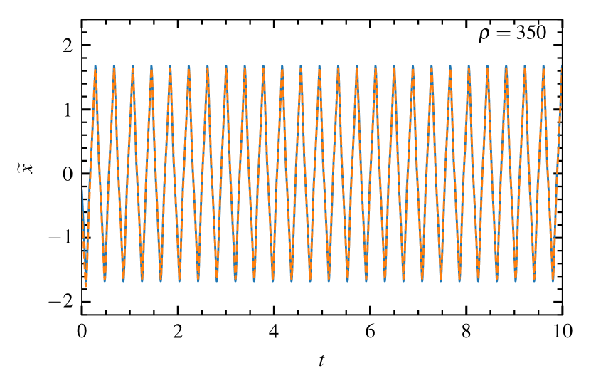
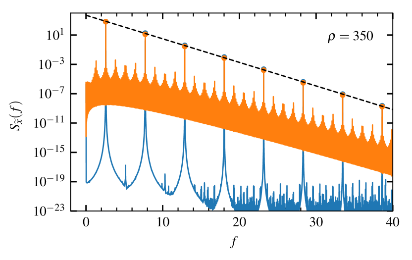
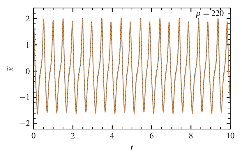
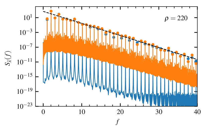
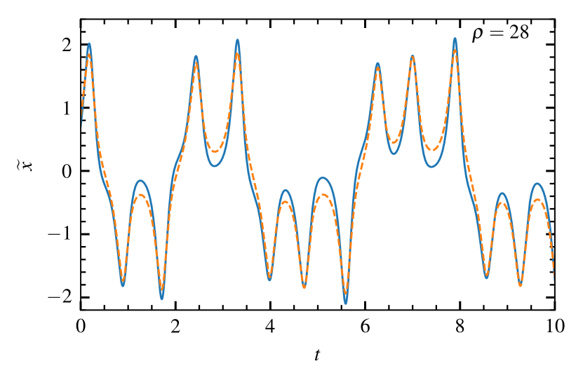
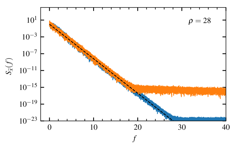
Figure 6: In blue: Excerpts of time seies of the $\widetilde{x}$-variable of the Lorenz system (left) with corresponding power spectral densities (right) for different values of the parameter $\rho$. These are compared to fits (orange lines) consisting of a superposition of skewed Lorentzian pulses. The fit is described in the text.

Table 1: Fit parameters for the time series in Fig. 6. $b^{+}$ denotes scaling of positive pulses, relative to the maxima in the time series, and $b^{-}$ denotes scaling of negative pulses. $\sigma$ and $\lambda$ are respectively the pulse asymmetry and location parameters for the asymmetric Lorentzian pulse described in App. F.1. The decay in the power spectral frequency $a$ and the pulse duration time $\tau_{\text{d}}=a/4\pi$ are given for completeness.

$\rho$	$b^{+}$	$b^{-}$	$\lambda$	$\sigma$	$a$	$\tau_{\text{d}}$
28	1.01	1.00	0.18	$-0.10$	1.9	0.15
220	1.13	0.87	0.27	$-0.12$	0.76	0.06
350	1.00	1.00	0.11	$-0.06$	0.74	0.06

Now we turn to the question of how the spectral peaks associated with periodicity in the time series vanish in the chaotic case. Interpreting the signal as a pulse train, we see quasi-periodic pulses with both positive and negative amplitudes and a mean waiting time between pulses $\langle\tau\rangle=0.75$. The quasi-periodic waiting time distribution alone should lead to the loss of all but a few spectral peaks as described in Sec. V. This effect is demonstrated on the left-hand side of Fig. 7. Here, the estimated forcing time series for $\rho=28$ (blue) is plotted along with the same time series where all amplitudes are set to 1 (orange). The quasi-periodicity is visible as a few broad spectral peaks where the first is approximately at $f=1/\langle\tau\rangle$. On the right-hand side of Fig. 7, the waiting time distribution is seen to be close to a log-normal distribution with scale parameter $0.13$, shape parameter $0.74$ and location parameter $0.6$. This parameterization of the log-normal distribution is presented in App. I.3. The distribution is broad enough to remove most of the spectral peaks.

Considering the amplitudes, we recall that from Eq. (23), the spectral peaks vanish if the mean value of the pulses disappears. This equation rests on the assumption that the amplitudes are pairwise uncorrelated and independent of the arrival and waiting times. In the chaotic case, the mean values of the amplitudes is indeed approximately zero ($\mathopen{}\mathclose{{}\left<A}\right>=0.01$). In Fig. 8, we investigate the two assumptions. On the left hand side, the auto-correlation function of the amplitudes is presented as a function of the pulse number. The function goes below 0.1 at the second lag, demonstrating that the amplitudes are indeed pairwise uncorrelated. On the right hand side of figure Fig. 8, we present a scatter plot of waiting times and the following pulse amplitudes. To demonstrate the symmetry of this plot, we also show the sign-reversed amplitudes. While the dependence between amplitudes and waiting times is complex, the relationship is also highly symmetric. Thus any waiting time has an equal probability of being followed by a positive or negative amplitude of equal magnitude. The correlation between the two variables is therefore low, even if they are dependent variables.

In conclusion, the broad (compared to a sum of delta functions) log-normal distribution of the waiting times ensures that most of the periodic spectral peaks are removed from the forcing signal. The pairwise uncorrelated pulse amplitudes and symmetric joint distribution between amplitudes and waiting times then remove the rest of the spectral peaks, leaving a flat forcing signal. Convolving this forcing signal with an asymmetric Lorentzian pulse function recovers the characteristic exponentially decaying PSD.

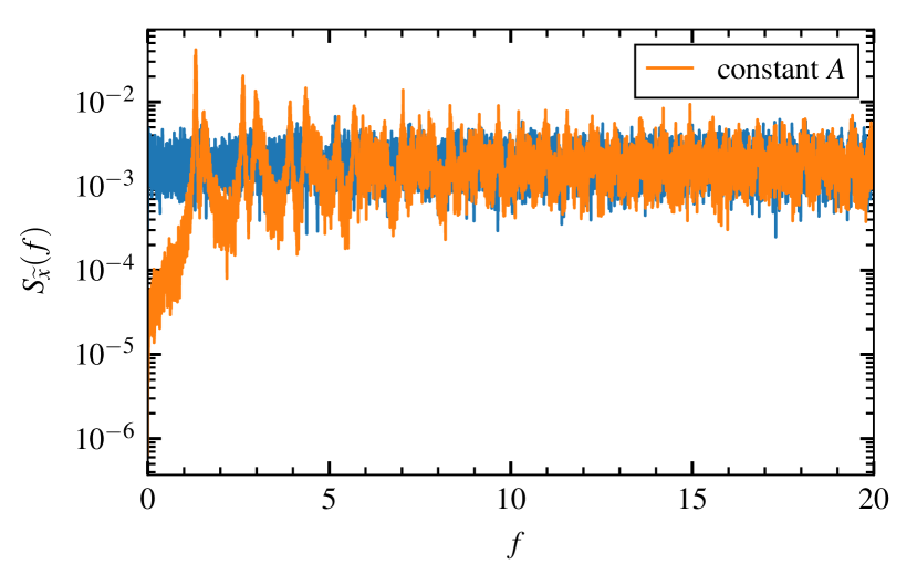
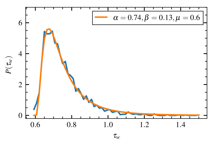
Figure 7: Left: Power spectral density of forcing signal in the chaotic case (blue) and the same forcing signal with all amplitudes set to $1$ (orange). Right: The histogram of the waiting times between events in the chaotic case (blue) and a fit with a log-normal distribution (orange), see App. I.3.

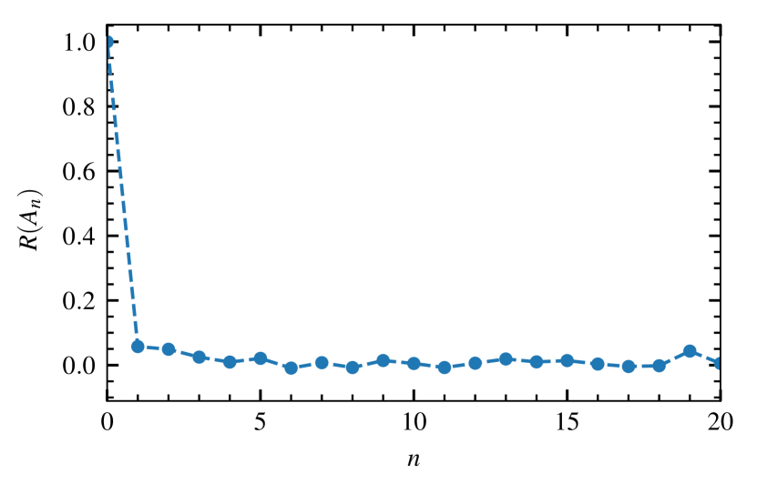
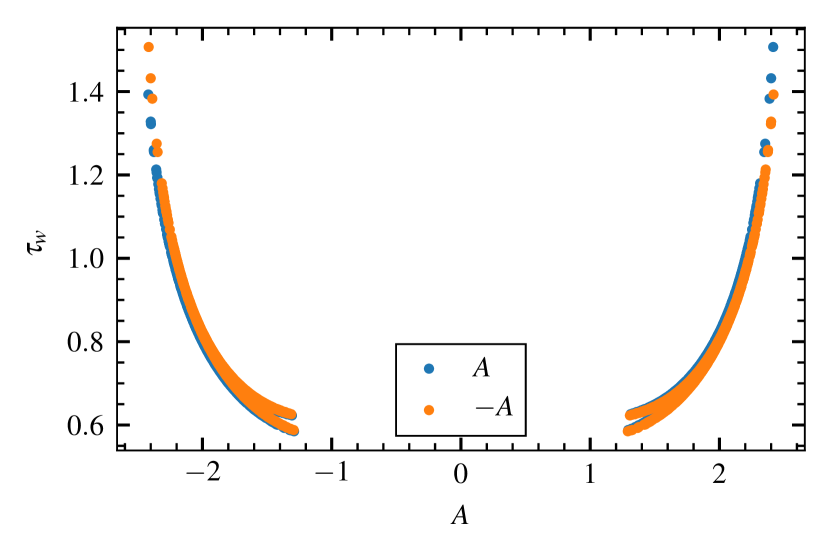
Figure 8: Left: Auto-correlation function of the sequence of pulse amplitudes in the chaotic case. Right: Scatter plot of pulse waiting times and the following amplitudes in the chaotic case. Original amplitudes are in blue, while the sign reversed amplitudes are in orange.

VII Conclusion

In this contribution, we have presented a stochastic model describing the power spectra of time series from non-linear dynamics and chaos as a super-position of pulses. The analytically investigated solutions comprise periodically arriving pulses, appropriate for non-linear oscillators, and pulses arriving according to a Poisson process, which is more appropriate for chaotic dynamics. For Poisson arrivals, the spectrum of the arrivals is flat while for periodic arrivals the spectrum is a Dirac comb. In both cases, the spectral decay is fully determined by the spectrum of the pulse function which simply modulates the spectrum of the arrivals. Results are also available for independent waiting times.[46, 43, 44, 45]

For strictly periodic or multi-periodic processes, the Dirac comb is a robust feature of the PSD, only removed by a vanishing mean of the pulse amplitudes. However, even for very modest deviations from strict periodicity, all harmonics except the lowest few are lost. This is true both for pulses randomly distributed around the periodic arrival time and for uni-modal and narrow waiting time distributions. This demonstrates why spectra in even quasi-periodic chaos do not display a Dirac comb in the PSD.

Asymmetric Lorentzian pulses with fixed pulse parameters have been shown to give a good description of the dynamics in the Lorenz system. The transition from periodic to multi-periodic oscillations is well described, and we have demonstrated that the loss of the Dirac comb in the chaotic regime is both due to deviations from the periodicity in the arrival times, as well as due to the lack of pairwise correlations between the pulse amplitudes and lack of correlation between pulse amplitudes and waiting times. This is true even though the joint distribution between pulse amplitudes and waiting times is highly nontrivial.

We have demonstrated that exponential spectra are a feature of nonlinear oscillations in general and that chaos is not a necessary condition for exponential decay of the PSD. Nonlinear, periodic oscillations can also give exponentially decaying power spectra, when the modulation of the spectrum Dirac comb is considered. Deviations from strict periodicity efficiently remove the Dirac comb, however, leaving only the exponential decay.

Data availability statement

The python code generating the presented Lorenz time traces and the associated fit functions are publicly available.[53]

Appendix A Simulations of the Lorenz model

The values of the model parameters and initial conditions used to generate the time series of the Lorenz model are presented in Table 2. For $\rho=28$ the model is run for a duration of 10 in order to reach the attractor. For $\rho=220$ and $\rho=350$ the initial values are already placed in the attractor. The analyzed time series have a duration of $10^{9}$ after the initial transient was removed. The Lorenz model is introduced in Sec. II and analyzed in Sec. VI.

$\rho$	$\sigma$	$\beta$	$x_{0}$	$y_{0}$	$z_{0}$
28	10	8/3	-4	-7	25
220	10	8/3	45	60	275
350	10	8/3	-8	-46	284

Table 2: Model parameters and initial conditions for numerical simulations of the Lorenz model.

Appendix B Fourier transform and power spectral density

The PSD of a random process $\Phi_{K}(t)$ on a domain of duration $T$ is defined as

$$\mathcal{S}_{\Phi_{K}}(\omega)=\lim_{T\to\infty}\frac{1}{T}\mathopen{}\mathclose{{}\left<\lvert\mathcal{F}_{T}\mathopen{}\mathclose{{}\left[{\Phi_{K}}}\right](\omega)\rvert^{2}}\right>,$$ (50)

where the angular brackets denote an average over all random variables and

$$\mathcal{F}_{T}\mathopen{}\mathclose{{}\left[{\Phi_{K}}}\right](\omega)=\int\limits_{-T/2}^{T/2}\text{d}t\,\exp(-i\omega t)\Phi_{K}(t)$$ (51)

is the finite-time Fourier transform of the random variable over the domain $[-T/2,T/2]$.

Analytical functions which fall sufficiently rapidly to zero (such as the pulse function $\varphi$) have the Fourier transform

$$\mathcal{F}\mathopen{}\mathclose{{}\left[{\varphi}}\right](\theta)=\int\limits_{-\infty}^{\infty}\text{d}s\,\varphi(s)\exp(-i\theta s)$$ (52)

and the inverse transform

$$\varphi(s)=\mathcal{F}^{-1}\mathopen{}\mathclose{{}\left[{\mathcal{F}\mathopen{}\mathclose{{}\left[{\varphi}}\right](\theta)}}\right](s)=\frac{1}{2\pi}\int\limits_{-\infty}^{\infty}\text{d}\theta\,\exp(i\theta s)\mathcal{F}\mathopen{}\mathclose{{}\left[{\varphi}}\right](\theta).$$ (53)

Note that here, $\theta$ and $s$ are non-dimensional variables, as opposed to $t$ and $\omega$.

Appendix C Periodic pulse arrivals

Here, we define the periodic pulse arrivals and provide the distribution of the counting process $K$. Here we will make use of the floor function $\mathopen{}\mathclose{{}\left\lfloor\cdot}\right\rfloor$. For simplicity of notation, we consider pulses which arrive in the interval $[0,T]$ and are distributed according to

$$P_{t_{k}|r}\mathopen{}\mathclose{{}\left(t_{k}|r;k}\right)=\delta\mathopen{}\mathclose{{}\left(t_{k}-\tau_{\text{p}}k+r}\right).$$ (54)

Here, $r$ is a random starting point, uniformly distributed on $[0,\tau_{\text{p}}]$. This is required to have time-independent ensemble statistics for the FPP. It is straightforward to see that all waiting times are identically and degenerately distributed, $t_{k+1}-t_{k}=\tau_{\text{p}}$ (assuming the arrival times are sorted).

Now we determine the number of arrivals $K(T)$. First note that if $T/\tau_{\text{p}}$ is an integer and $r=0$, we have arrivals at $0$ and at $T$, giving $K=T/\tau_{\text{p}}$ arrivals. If $r>0$, we loose the last arrival and there are $K=T/\tau_{\text{p}}-1$ arrivals. Since $r=0$ happens with probability 0, we almost surely have $T/\tau_{\text{p}}-1$ arrivals. If $T/\tau_{\text{p}}$ is not an integer, note that $T/\tau_{\text{p}}-\mathopen{}\mathclose{{}\left\lfloor T/\tau_{\text{p}}}\right\rfloor$ is a number between 0 and 1. As long as $r/\tau_{\text{p}}<T/\tau_{\text{p}}-\mathopen{}\mathclose{{}\left\lfloor T/\tau_{\text{p}}}\right\rfloor$, we can fit $K=\mathopen{}\mathclose{{}\left\lfloor T/\tau_{\text{p}}}\right\rfloor$ events into the time window, the first at $r$ and the last at $\tau_{\text{p}}\mathopen{}\mathclose{{}\left\lfloor T/\tau_{\text{p}}}\right\rfloor+r<T$. Since $r$ is uniformly distributed on $[0,\tau_{\text{p}}]$, this happens with probability $T/\tau_{\text{p}}-\mathopen{}\mathclose{{}\left\lfloor T/\tau_{\text{p}}}\right\rfloor$. Otherwise, we have one less event and $K=\mathopen{}\mathclose{{}\left\lfloor T/\tau_{\text{p}}}\right\rfloor-1$. This agrees with the above, since if $T/\tau_{\text{p}}$ is an integer, $T/\tau_{\text{p}}=\mathopen{}\mathclose{{}\left\lfloor T/\tau_{\text{p}}}\right\rfloor$ and the probability of $T/\tau_{\text{p}}$ events goes to $0$. Thus we see that the probability mass function of $K$ is

$$P_{K}(k;T,\tau_{\text{p}})=\begin{cases}1-(T/\tau_{\text{p}}-\mathopen{}\mathclose{{}\left\lfloor T/\tau_{\text{p}}}\right\rfloor),&k=\mathopen{}\mathclose{{}\left\lfloor T/\tau_{\text{p}}}\right\rfloor-1\\ T/\tau_{\text{p}}-\mathopen{}\mathclose{{}\left\lfloor T/\tau_{\text{p}}}\right\rfloor,&k=\mathopen{}\mathclose{{}\left\lfloor T/\tau_{\text{p}}}\right\rfloor\end{cases}$$ (55)

This gives $\langle K\rangle=T/\tau_{\text{p}}-1$ and $K_{\text{rms}}^{2}=(T/\tau_{\text{p}}-\mathopen{}\mathclose{{}\left\lfloor T/\tau_{\text{p}}}\right\rfloor)(1+\mathopen{}\mathclose{{}\left\lfloor T/\tau_{\text{p}}}\right\rfloor-T/\tau_{\text{p}})$. Note that $K_{\text{rms}}^{2}$ is bounded: writing $T/\tau_{\text{p}}=\mathopen{}\mathclose{{}\left\lfloor T/\tau_{\text{p}}}\right\rfloor+\epsilon$ where $0\leq\epsilon<1$, we have $K_{\text{rms}}^{2}=\epsilon(1-\epsilon)$. In this contribution, we are mainly interested in the limit $T/\tau_{\text{p}}\gg 1$, in which case simply setting $K(T)=\mathopen{}\mathclose{{}\left\lfloor T/\tau_{\text{p}}}\right\rfloor$ is a good approximation.

The periodic pulse arrival time distribution is used in Sec. III.2.2 and V.2.

Appendix D Extended Campbell’s theorem

For a full discussion of Campbell’s theorem for the mean value of a shot noise process as well as various extensions, we refer to Refs. 51, 32, 33, 52. It can be shown that for independent and identically distributed (i.i.d.) waiting times $W$ with distribution $p_{W}$ and mean value $\tau_{w}$, we have in our notation

$$\mathopen{}\mathclose{{}\left<\Phi^{2}}\right>=\gamma\mathopen{}\mathclose{{}\left<A^{2}}\right>I_{2}+\\ 2\gamma\mathopen{}\mathclose{{}\left<A}\right>^{2}I_{2}\sum_{k=1}^{\infty}\int_{0}^{\infty}\text{d}w_{1}\,\cdots\int_{0}^{\infty}\text{d}w_{k}P_{W}(w_{1})\cdots P_{W}(w_{k})\rho_{\varphi}\mathopen{}\mathclose{{}\left(\frac{1}{\tau_{\text{d}}}\sum_{n=1}^{k}w_{n}}\right).$$ (56)

The $k$’th order integral can be compactly written as $\mathopen{}\mathclose{{}\left<\rho_{\phi}(S_{k}/\tau_{\text{d}})}\right>$, where $S_{k}=\sum_{n=1}^{k}w_{n}$. All $w_{n}$ are i.i.d., with distribution $p_{W}$, and we denote the corresponding characteristic function as $C_{W}$. We get

$$\mathopen{}\mathclose{{}\left<\rho_{\varphi}\mathopen{}\mathclose{{}\left(\frac{1}{\tau_{\text{d}}}S_{k}}\right)}\right> =\int\limits_{-\infty}^{\infty}\text{d}S\,P_{S}(S;k)\rho_{\varphi}\mathopen{}\mathclose{{}\left(\frac{1}{\tau_{\text{d}}}S}\right)$$

$$=\frac{1}{2\pi}\int\limits_{-\infty}^{\infty}\text{d}u\,\int\limits_{-\infty}^{\infty}\text{d}S\,C_{S}(u;k)\exp(-iSu)\rho_{\varphi}\mathopen{}\mathclose{{}\left(\frac{1}{\tau_{\text{d}}}S}\right).$$ (57)

As $C_{S}$ is the characteristic function of the sum of $k$ i.i.d. random variables, we get $C_{S}(u;k)=C_{W}(u)^{k}$. Further, we see that this equation contains the Fourier transform of $\rho_{\varphi}$, so we have

$$\mathopen{}\mathclose{{}\left<\rho_{\varphi}\mathopen{}\mathclose{{}\left(\frac{1}{\tau_{\text{d}}}S_{k}}\right)}\right>=\frac{\tau_{\text{d}}}{2\pi}\int\limits_{-\infty}^{\infty}\text{d}u\,C_{W}(u)^{k}\varrho_{\varphi}\mathopen{}\mathclose{{}\left(\tau_{\text{d}}u}\right),$$ (58)

which gives

$$\mathopen{}\mathclose{{}\left<\Phi^{2}}\right>=\gamma\mathopen{}\mathclose{{}\left<A^{2}}\right>I_{2}+2\gamma\mathopen{}\mathclose{{}\left<A}\right>^{2}I_{2}\sum_{k=1}^{\infty}\frac{\tau_{\text{d}}}{2\pi}\int\limits_{-\infty}^{\infty}\text{d}u\,C_{W}(u)^{k}\varrho_{\varphi}\mathopen{}\mathclose{{}\left(\tau_{\text{d}}u}\right).$$ (59)

For periodic arrivals, $P_{W}(w)=\delta(w-\tau_{w})$, giving $C_{W}(u)=\exp(iu\tau_{w})$, and we get

$$\mathopen{}\mathclose{{}\left<\Phi^{2}}\right>=\gamma\mathopen{}\mathclose{{}\left<A^{2}}\right>I_{2}+\\ 2\gamma\mathopen{}\mathclose{{}\left<A}\right>^{2}I_{2}\sum_{k=1}^{\infty}\rho_{\varphi}\mathopen{}\mathclose{{}\left(\frac{1}{\tau_{\text{d}}}k\tau_{\text{w}}}\right).$$ (60)

As $A_{\text{rms}}^{2}=\mathopen{}\mathclose{{}\left<A^{2}}\right>-\mathopen{}\mathclose{{}\left<A}\right>^{2}=\mathopen{}\mathclose{{}\left<A^{2}}\right>-\mathopen{}\mathclose{{}\left<A}\right>^{2}\rho_{\varphi}(0)$ and $\rho_{\varphi}(s)=\rho_{\varphi}(-s)$, this is equivalent to Eq. (44).

Appendix E Poisson summation formula

Here, we briefly present the well-known Poisson summation formula, which is treated in a number of textbooks, see Refs. 54, 55, 56, 57. For our purposes, the formulation used in Corollary VII.2.6 in Ref. 55 is the most useful. The statement in the book is for functions on general Euclidian spaces, but we repeat it here only for our special case (the real line):

Suppose the Fourier transform of the function $h$ and its inverse are defined as in Eqs. (52) and (53), respectively. Further suppose that $\lvert h(s)\rvert\leq A(1+\lvert s\rvert)^{-1-\delta}$ and $\lvert\mathcal{F}\mathopen{}\mathclose{{}\left[{h}}\right](\theta)\rvert\leq A(1+\lvert\theta/2\pi\rvert)^{-1-\delta}$ with $A>0$ and $\delta>0$. Then

$$\sum\limits_{m=-\infty}^{\infty}h(m)=\sum\limits_{n=-\infty}^{\infty}\mathcal{F}\mathopen{}\mathclose{{}\left[{h}}\right](2\pi n),$$ (61)

where both series converge absolutely.

• Note that the inequality conditions guarantee that both $\lvert h(s)\rvert$ and $\lvert\mathcal{F}\mathopen{}\mathclose{{}\left[{h}}\right](\theta)\rvert$ are integrable, which again guarantees that both $h$ and its Fourier transform are continuous and vanish at infinity (Theorem I.1.2 in Ref. 55)).

• Using properties of the Fourier transform, the summation formula can be cast to a number of different forms:

  $$\sum\limits_{n=-\infty}^{\infty}\mathcal{F}\mathopen{}\mathclose{{}\left[{h}}\right](2\pi n) =\sum\limits_{m=-\infty}^{\infty}h(m),$$ (62)

  $$\sum\limits_{n=-\infty}^{\infty}\gamma\mathcal{F}\mathopen{}\mathclose{{}\left[{h}}\right](2\pi n\gamma) =\sum\limits_{m=-\infty}^{\infty}h(m/\gamma),$$ (63)

  $$\sum\limits_{n=-\infty}^{\infty}\gamma\mathcal{F}\mathopen{}\mathclose{{}\left[{h}}\right](2\pi n\gamma)\exp(i2\pi n\gamma t/\tau_{\text{d}}) =\sum\limits_{m=-\infty}^{\infty}h(m/\gamma+t/\tau_{\text{d}}).$$ (64)

• By using the definitions of $\rho$ and $\varrho$ given in Eqs. (9) and (10), respectively, as well as the Fourier transform, we have that if Eq. (61) holds for $\varphi$, then by Eq. (64) we have

  $$\sum\limits_{m=-\infty}^{\infty}\varphi(m+s) =\sum\limits_{n=-\infty}^{\infty}\mathcal{F}\mathopen{}\mathclose{{}\left[{\varphi}}\right](2\pi n)\exp(i2\pi ns),$$

  $$\int\limits_{-\infty}^{\infty}\text{d}u\,\varphi(u)\sum\limits_{m=-\infty}^{\infty}\varphi(s+m) =\int\limits_{-\infty}^{\infty}\text{d}u\,\varphi(u)\sum\limits_{m=-\infty}^{\infty}\mathcal{F}\mathopen{}\mathclose{{}\left[{\varphi}}\right](2\pi n)\exp(i2\pi ns),$$

  $$\sum\limits_{m=-\infty}^{\infty}\rho_{\varphi}(m) =\sum\limits_{n=-\infty}^{\infty}\varrho_{\varphi}(2\pi n),$$

  which means that the summation formula holds for the correlation function and power spectrum of the pulse as well. This does not necessarily work in reverse - if one of the sums over $\varphi$ or its Fourier transform diverges, we cannot exchange the summation and the integral in the second step.

The Poisson summation formula is used to compute the auto-correlation function from the PSD in Sec. IV.2.

Appendix F Lorentzian pulse function

Throughout this contribution, we use Lorentzian pulse functions to illustrate the exponential spectral decay observed in nonlinear oscillations and chaotic dynamics. Here, we present this pulse function and its properties.

The simple Lorentzian pulse is given by

$$\varphi(s)=\frac{1}{\pi(1+s^{2})}.$$ (65)

Its Fourier transform is

$$\mathcal{F}\mathopen{}\mathclose{{}\left[{\varphi}}\right](\theta)=\exp(-\lvert\theta\rvert),$$ (66)

the integrals are[30]

$$I_{n}=\frac{\Gamma(n-1/2)}{\pi^{n-1/2}\Gamma(n)},$$ (67)

and we have the pulse auto-correlation function

$$\rho_{\varphi}(s)=\frac{4}{4+s^{2}},$$ (68)

and spectrum

$$\varrho_{\varphi}(\theta)=2\pi\exp(-2\lvert\theta\rvert).$$ (69)

In general, the full sum of the correlation function is given by

$$\sum\limits_{m=-\infty}^{\infty}\rho_{\varphi}\mathopen{}\mathclose{{}\left(\frac{m}{\gamma}+\frac{t}{\tau_{\text{d}}}}\right)=\gamma\pi\mathopen{}\mathclose{{}\left[\coth(2\gamma\pi-i\gamma\pi t/\tau_{\text{d}})+\coth(2\gamma\pi+i\gamma\pi t/\tau_{\text{d}})}\right].$$ (70)

Two special cases of this are of interest here. For $t=0$, we get

$$\sum\limits_{m=-\infty}^{\infty}\rho_{\varphi}\mathopen{}\mathclose{{}\left(\frac{m}{\gamma}}\right)=2\gamma\pi\coth(2\gamma\pi),$$ (71)

while in the limit $\gamma\to 0$ we get the expected result

$$\lim_{\gamma\to 0}\sum\limits_{m=-\infty}^{\infty}\rho_{\varphi}\mathopen{}\mathclose{{}\left(\frac{m}{\gamma}+\frac{t}{\tau_{\text{d}}}}\right)=\rho_{\varphi}(t/\tau_{\text{d}}).$$ (72)

F.1 The localized and asymmetric Lorentzian pulse

A generalization of the basic Lorentzian pulse with the same PSD as the basic Lorentzian pulse is based on the theory of stable distributions. It has no general closed analytic form, but its Fourier transform is given by[20, 29]

$$\mathcal{F}\mathopen{}\mathclose{{}\left[{\varphi}}\right](\theta;\sigma,\mu)=\exp(-\lvert\theta\rvert)\exp\mathopen{}\mathclose{{}\left(\text{i}\mu\theta-\text{i}\frac{2\sigma}{\pi}\theta\ln\lvert\theta\rvert}\right),$$ (73)

where $-1\leq\sigma\leq 1$ is an asymmetry parameter and $\mu\in\mathbb{R}$ is a location parameter. In the case $\sigma=\mu=0$, this pulse reduces to the basic Lorentzian pulse given by Eq. (65).

For all choices of $\sigma$ and $\mu$, the power spectrum and correlation function is identical to that of the basic Lorentzian pulse, and so the above results for the Poisson summation holds. Consistently, $I_{1}$ and $I_{2}$ coincide for all choices of $\sigma$ and $\mu$.

Appendix G Representation of the Dirac delta function

A basic theorem in the theory of distributions is Theorem 2.5 in Ref. 58: Let $h(x)$ be a piecewise continuous function such that:

• $\int_{-\infty}^{\infty}\text{d}x\,\mathopen{}\mathclose{{}\left|h(x)}\right|<\infty$,

• $\int_{-\infty}^{\infty}\text{d}x\,h(x)=1$.

Writing $h_{a}(x)=ah(ax)$, we have that

$$h_{a}(x)\to\delta(x)\quad\text{as}\quad a\to\infty.$$ (74)

In particular, we note that

$$h(x)=\frac{1-\cos(x)}{\pi x^{2}}$$ (75)

fulfills the requirements of the theorem.

Appendix H Representation of delta functions under finite sampling

For graphical presentation of Dirac delta functions, we use its discrete analog, the Kronecker delta. For $t\to t_{n}\triangle_{\text{t}}n$, we have $\omega\to 2\pi f_{m}=2\pi m/\triangle_{\text{t}}$, where $n$ and $m$ are integers. A Dirac delta at a given angular frequency $\omega_{*}$ is then given by $\delta(\omega-\omega_{*})=\delta(2\pi(m-k)/\triangle_{\text{t}})=\frac{\triangle_{\text{t}}}{2\pi}\delta_{m-k}$ where $k$ is the nearest integer to $\triangle_{\text{t}}\omega_{*}/2\pi$. That is, the Dirac delta is approximated as a boxcar of width equal to the sampling time and an amplitude equal to the inverse of the sampling time. This indicates the amplitude of the delta spikes, separates them from any superposed functions and tends to better approximations for finer sampling.

Appendix I Probability distributions

Here, we present some selected probability distributions with varying definitions in the literature. In the following, $X$ is a random variable and $x$ is the value it takes.

I.1 Gamma distribution

The Gamma distribution with scale parameter $\theta>0$ and shape parameter $\beta>0$ is defined for positive argument $x>0$, and is given by

$$p_{X}(x;\beta,\theta)=\frac{x^{\beta-1}}{\theta^{\beta}\Gamma(\beta)}\exp\mathopen{}\mathclose{{}\left(-\frac{x}{\theta}}\right).$$ (76)

Here, $\Gamma$ is the Gamma function.

I.2 Asymmetric Laplace distribution

We choose a parametrization which has the exponential distribution as a straightforward limit.[59] Here, $\alpha>0$ is a scale parameter and $0<\lambda<1$ is an asymmetry parameter,

$$p_{X}(x;\alpha,\lambda)=\frac{1}{2\alpha}\begin{cases}\exp\mathopen{}\mathclose{{}\left(-\frac{A}{2\alpha(1-\lambda)}}\right),&A>0\\ \exp\mathopen{}\mathclose{{}\left(\frac{A}{2\alpha\lambda}}\right),&A<0\\ \end{cases}$$ (77)

I.3 Log-normal distribution

The log-normal distribution with shape parameter $\alpha$, scale parameter $\beta$ and location parameter $\mu$ is given by [60]

$$p_{X}(x;\alpha,\beta,\mu)=\frac{1}{\alpha(x-\mu)\sqrt{2\pi}}\mathrm{exp}\mathopen{}\mathclose{{}\left(-\frac{\mathrm{log}^{2}\mathopen{}\mathclose{{}\left((x-\mu)/\beta}\right)}{2\alpha^{2}}}\right).$$ (78)

References

- Atten et al. [1980] P. Atten, J. Lacroix, and B. Malraison, Phys. Lett. A 79, 255 (1980).
- Frisch and Morf [1981] U. Frisch and R. Morf, Phys. Rev. A 23, 2673 (1981).
- Greenside et al. [1982] H. Greenside, G. Ahlers, P. Hohenberg, and R. Walden, Physica D 5, 322 (1982).
- Broomhead and King [1986] D. Broomhead and G. P. King, Physica D 20, 217 (1986).
- Brandstater and Swinney [1987] A. Brandstater and H. L. Swinney, Phys. Rev. A 35, 2207 (1987).
- Streett and Hussaini [1991] C. Streett and M. Hussaini, Appl. Numer. Math 7, 41 (1991).
- Sigeti [1995a] D. E. Sigeti, Physica D 82, 136 (1995a).
- Sigeti [1995b] D. E. Sigeti, Phys. Rev. E 52, 2443 (1995b).
- Paul et al. [2001] M. R. Paul, M. C. Cross, P. F. Fischer, and H. S. Greenside, Phys. Rev. Lett. 87, 154501 (2001).
- Franzke et al. [2015] C. L. E. Franzke, S. M. Osprey, P. Davini, and N. W. Watkins, Sci Rep 5, 9068 (2015).
- Pace et al. [2008a] D. C. Pace, M. Shi, J. E. Maggs, G. J. Morales, and T. A. Carter, Phys. Rev. Lett. 101, 085001 (2008a).
- Pace et al. [2008b] D. C. Pace, M. Shi, J. E. Maggs, G. J. Morales, and T. A. Carter, Phys. Plasmas 15, 122304 (2008b).
- Hornung et al. [2011] G. Hornung, B. Nold, J. E. Maggs, G. J. Morales, M. Ramisch, and U. Stroth, Phys. Plasmas 18, 082303 (2011).
- Maggs and Morales [2012a] J. E. Maggs and G. J. Morales, Phys. Rev. E 86, 015401 (2012a).
- Maggs et al. [2015] J. E. Maggs, T. L. Rhodes, and G. J. Morales, Plasma Phys. Control. Fusion 57, 045004 (2015).
- Zhu et al. [2017] Z. Zhu, A. E. White, T. A. Carter, S. G. Baek, and J. L. Terry, Phys. Plasmas 24, 042301 (2017).
- Decristoforo et al. [2020] G. Decristoforo, A. Theodorsen, and O. E. Garcia, Phys. Fluids 32, 085102 (2020).
- Decristoforo et al. [2021] G. Decristoforo, A. Theodorsen, J. Omotani, T. Nicholas, and O. E. Garcia, Phys. Plasmas 28, 072301 (2021).
- Ohtomo et al. [1995] N. Ohtomo, K. Tokiwano, Y. Tanaka, A. Sumi, S. Terachi, and H. Konno, J. Phys. Soc. Jpn. 64, 1104 (1995).
- Maggs and Morales [2011] J. E. Maggs and G. J. Morales, Phys. Rev. Lett. 107, 185003 (2011).
- Maggs and Morales [2012b] J. E. Maggs and G. J. Morales, Plasma Phys. Control. Fusion 54, 124041 (2012b).
- Doyne Farmer [1982] J. Doyne Farmer, Physica D 4, 366 (1982).
- Libchaber et al. [1983] A. Libchaber, S. Fauve, and C. Laroche, Physica D 7, 73 (1983).
- Stone [1990] E. F. Stone, Phys. Lett. A 148, 434 (1990).
- Klinger et al. [1997] T. Klinger, A. Latten, A. Piel, G. Bonhomme, T. Pierre, and T. Dudok de Wit, Phys. Rev. Lett. 79, 3913 (1997).
- Mensour and Longtin [1998] B. Mensour and A. Longtin, Physica D 113, 1 (1998).
- Safonov et al. [2002] L. A. Safonov, E. Tomer, V. V. Strygin, Y. Ashkenazy, and S. Havlin, Chaos 12, 1006 (2002).
- Garcia and Theodorsen [2017a] O. E. Garcia and A. Theodorsen, Phys. Plasmas 24, 020704 (2017a).
- Garcia and Theodorsen [2018a] O. E. Garcia and A. Theodorsen, Phys. Plasmas 25, 014503 (2018a).
- Garcia et al. [2018] O. E. Garcia, R. Kube, A. Theodorsen, B. LaBombard, and J. L. Terry, Phys. Plasmas 25, 056103 (2018).
- Parzen [1999] E. Parzen, Stochastic Processes (Society for Industrial and Applied Mathematics, 1999).
- Pécseli [2000] H. L. Pécseli, Fluctuations in Physical Systems (Cambridge University Press, Cambridge ; New York, 2000).
- Rice [1944] S. O. Rice, Bell Syst. Tech. J. 23, 282 (1944).
- Garcia [2012] O. E. Garcia, Phys. Rev. Lett. 108, 265001 (2012).
- Garcia et al. [2015] O. Garcia, J. Horacek, and R. Pitts, Nucl. Fusion 55, 062002 (2015).
- Theodorsen et al. [2016] A. Theodorsen, O. E. Garcia, J. Horacek, R. Kube, and R. A. Pitts, Plasma Phys. Control. Fusion 58, 044006 (2016).
- Garcia et al. [2017] O. Garcia, R. Kube, A. Theodorsen, J.-G. Bak, S.-H. Hong, H.-S. Kim, t. K. P. Team, and R. Pitts, Nucl. Mater. Energy 12, 36 (2017).
- Walkden et al. [2017] N. R. Walkden, A. Wynn, F. Militello, B. Lipschultz, G. Matthews, C. Guillemaut, J. Harrison, D. Moulton, and JET Contributors, Plasma Phys. Control. Fusion 59, 085009 (2017).
- Theodorsen et al. [2017a] A. Theodorsen, O. Garcia, R. Kube, B. LaBombard, and J. Terry, Nucl. Fusion 57, 114004 (2017a).
- Garcia and Theodorsen [2018b] O. E. Garcia and A. Theodorsen, Phys. Plasmas 25, 014506 (2018b).
- Theodorsen et al. [2018] A. Theodorsen, O. E. Garcia, R. Kube, B. LaBombard, and J. L. Terry, Phys. Plasmas 25, 122309 (2018).
- Bencze et al. [2019] A. Bencze, M. Berta, A. Buzás, P. Hacek, J. Krbec, M. Szutyányi, and the COMPASS Team, Plasma Phys. Control. Fusion 61, 085014 (2019).
- Brunsden et al. [1989] V. Brunsden, J. Cortell, and P. J. Holmes, J. Sound Vib. 130, 1 (1989).
- Brunsden and Holmes [1987] V. Brunsden and P. Holmes, Phys. Rev. Lett. 58, 1699 (1987).
- Holmes et al. [1996] P. Holmes, J. L. Lumley, and G. Berkooz, Turbulence, Coherent Structures, Dynamical Systems and Symmetry, Cambridge Monographs on Mechanics (Cambridge University Press, Cambridge, 1996).
- Lowen and Teich [2005] S. B. Lowen and M. C. Teich, Fractal-Based Point Processes (Wiley-Interscience, Hoboken, N.J, 2005).
- Lorenz [1963] E. N. Lorenz, J. Atmos. Sci. 20, 130 (1963).
- Garcia et al. [2016] O. E. Garcia, R. Kube, A. Theodorsen, and H. L. Pécseli, Phys. Plasmas 23, 052308 (2016).
- Garcia and Theodorsen [2017b] O. E. Garcia and A. Theodorsen, Phys. Plasmas 24, 032309 (2017b).
- Theodorsen et al. [2017b] A. Theodorsen, O. E. Garcia, and M. Rypdal, Phys. Scr. 92, 054002 (2017b).
- Campbell [1909a] N. Campbell, Math. Proc. Camb. Phil. Soc. 15, 310 (1909a).
- Campbell [1909b] N. Campbell, Math. Proc. Camb. Phil. Soc. 15, 117 (1909b).
- pap [2022] https://github.com/uit-cosmo/Dirac-comb-and-exponential-frequency-spectra-in-nonlinear-dynamics (2022), retrieved 07-11-2022.
- Bochner et al. [1959] S. Bochner, M. Tenenbaum, H. Pollard, and S. Bochner, Lectures on Fourier Integrals, Annals of Mathematic Studies No. 42 (Princeton Univ. Press, Princeton, NJ, 1959).
- Stein and Weiss [1975] E. M. Stein and G. Weiss, Introduction to Fourier Analysis on Euclidean Spaces, Princeton Mathematical Series No. 32 (Princeton University Press, Princeton, N.J, 1975).
- Grafakos [2009] L. Grafakos, Classical Fourier Analysis, Graduate Texts in Mathematics, Vol. 249 (Springer New York, New York, NY, 2009).
- Overholt [2014] M. Overholt, A Course in Analytic Number Theory, Graduate Studies in Mathematics No. volume 160 (American Mathematical Society, Providence, Rhode Island, 2014).
- Richards and Youn [1990] J. I. Richards and H. K. Youn, The Theory of Distributions: A Nontechnical Introduction, 1st ed. (Cambridge University Press, 1990).
- Theodorsen and Garcia [2018] A. Theodorsen and O. E. Garcia, Plasma Phys. Control. Fusion 60, 034006 (2018).
- log [2022] https://docs.scipy.org/doc/scipy/reference/generated/scipy.stats.lognorm.html (2022), retrieved 07-11-2022.