HySPA: Hybrid Span Generation for Scalable Text-to-Graph Extraction

Abstract

Text-to-Graph extraction aims to automatically extract information graphs consisting of mentions and types from natural language texts. Existing approaches, such as table filling and pairwise scoring, have shown impressive performance on various information extraction tasks, but they are difficult to scale to datasets with longer input texts because of their second-order space/time complexities with respect to the input length. In this work, we propose a Hybrid SPan GenerAtor (HySPA) that invertibly maps the information graph to an alternating sequence of nodes and edge types, and directly generates such sequences via a hybrid span decoder which can decode both the spans and the types recurrently in linear time and space complexities. Extensive experiments on the ACE05 dataset show that our approach also significantly outperforms state-of-the-art on the joint entity and relation extraction task.

1 Introduction

Information Extraction (IE) can be viewed as a Text-to-Graph extraction task that aims to extract an information graph Li et al. (2014); Shi et al. (2017) consisting of mentions and types from unstructured texts, where the nodes of the graph are mentions or entity types and the edges are relation types that indicate the relations between the nodes. A typical approach towards graph extraction is to break the extraction process into sub-tasks, such as Named Entity Recognition (NER) Florian et al. (2006, 2010) and Relation Extraction (RE) Sun et al. (2011); Jiang and Zhai (2007), and either perform them separately Chan and Roth (2011) or jointly Li and Ji (2014); Eberts and Ulges (2019).

Recent joint IE models Wadden et al. (2019); Wang and Lu (2020); Lin et al. (2020) have shown impressive performance on various IE tasks, since they can mitigate error propagation and leverage inter-dependencies between the tasks. Previous work often uses pairwise scoring techniques to identify relation types between entities. However, this approach is computationally inefficient because it needs to enumerate all possible entity pairs in a document, and the relation type is a null value for most of the cases due to the sparsity of relations between entities. Also, pairwise scoring techniques evaluate each relation type independently and thus fail to capture interrelations between relation types for different pairs of mentions.

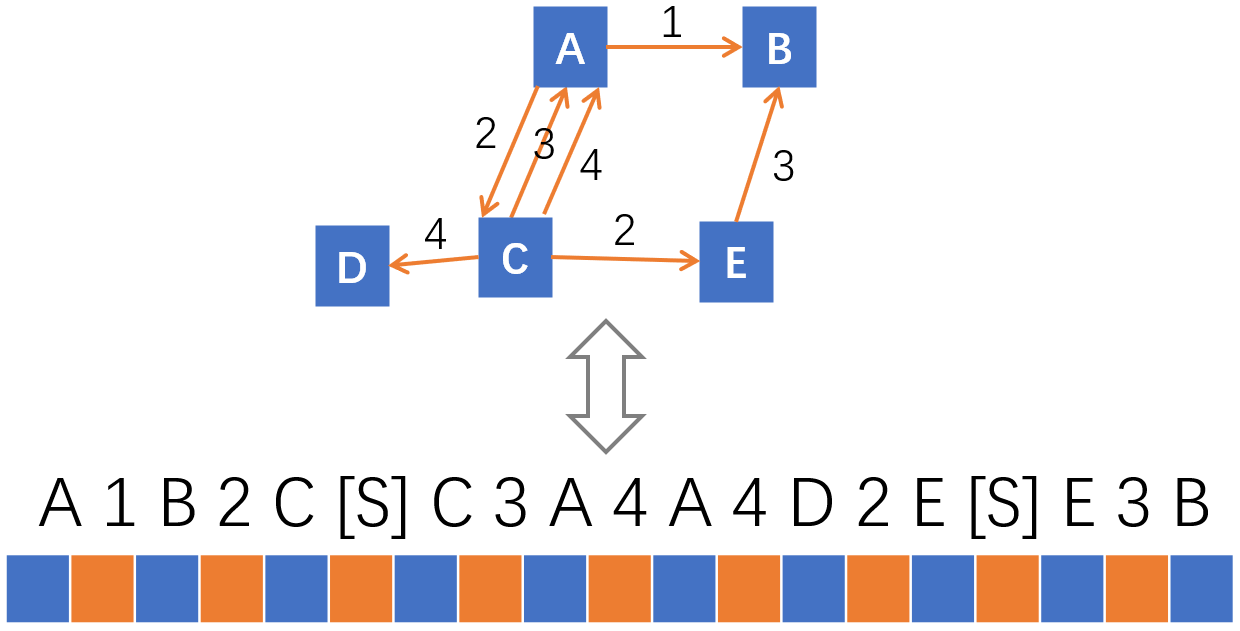
Figure 1: We represent directed multigraphs as alternating sequences of nodes (blue) and edges (orange). Here, the graph is traversed by Breadth First Search (BFS) with an ascending ordering of nodes and edge types. “[s]” or [SEP] is a virtual edge type, representing the end of each BFS level.

Another approach is to treat the joint information extraction task as a table filling problem Zhang et al. (2017); Wang and Lu (2020), and generate two-dimensional tables with a Multi-Dimensional Recurrent Neural Network Graves et al. (2007). This can capture interrelations among entities and relations, but the space complexity grows quadratically with respect to the length of the input text, making this approach impractical for long sequences.

Some attempts, such as Seq2RDF Liu et al. (2018) and IMoJIE Kolluru et al. (2020), leverage the power of Seq2seq models Cho et al. (2014) to capture the interrelations among mentions and types with first-order complexity, but they all use a pre-defined vocabulary for mention prediction, which largely depends on the distribution of the target words and will not be able to handle unseen out-of-vocabulary words.

To solve these problems, we propose a first-order approach that invertibly maps the target graph to an alternating sequence of nodes and edges, and applies a hybrid span generator that directly learns to generate such alternating sequences. Our main contributions are three-fold:

• We propose a general technique to invertibly map between an information graph and an alternating sequence (assuming a given graph traversal algorithm). Generating an alternating sequence is equivalent to generating the original information graph.

• We propose a novel neural decoder that is enforced to only generate alternating sequences by decoding spans and types in a hybrid manner. For each decoding step, our decoder only has linear space and time complexity with respect to the length of the input sequence, and it can capture inter-dependencies among mentions and types due to its nature as a sequential decision process.

• We conduct extensive experiments on the Automatic Content Extraction (ACE) dataset which show that our model achieves state-of-the-art performance on the joint entity and relation extraction task which aims to extract a knowledge graph from a piece of unstructured text.

2 Modeling Information Graphs as Alternating Sequences

An information graph can be viewed as a heterogeneous multigraph Li et al. (2014); Shi et al. (2017) $G=(V,E)$, where $V$ is a set of nodes (typically representing spans $(t_{s},t_{e})$ in the input document) and $E$ is a multiset of edges with a node type mapping function $\phi:V\rightarrow Q$ and an edge type mapping function $\psi:E\rightarrow R$. Node and edge types are assumed to be drawn from a finite vocabulary. Node types can be used e.g. to represent entity types (PER, ORG, etc.), while edge types may represent relations (PHYS, ORG-AFF, etc.) between the nodes. In this work, we represent node types as separate nodes that are connected to their node $v$ by a special edge type, [TYPE].

Representing information graphs as sequences

Instead of directly modeling the space of heterogeneous multigraphs, $\mathcal{G}$, we build a mapping $s^{\pi}=f_{s}(G,\pi)$ from $\mathcal{G}$, to a sequence space $S^{\pi}$. $f_{s}$ depends on a (given) ordering $\pi$ of nodes and their edges in $G$, constructed by a graph traversal algorithm like Breadth First Search (BFS) or Depth First Search (DFS), and an internal ordering of nodes and edge types. We assume that the elements $s^{\pi}_{i}$ of the resultant sequences $s^{\pi}$ are drawn from finite sets of node representations $V$ (defined below), node types $Q$, edge types $R$ (incl. [TYPE]), and “virtual” edge types $U$: $\forall~{}s_{i}^{\pi}\in~{}s^{\pi},~{}s_{i}^{\pi}\in V\cup Q\cup R\cup U$. Virtual edge types $U=\{\text{[SOS]},\text{[EOS]},\text{[SEP]}\}$ do not represent edges in $G$, but serve to control the generation of the sequence, indicating the start/end of sequences and the separation of levels in the graph.

We furthermore assume that $s^{\pi}=s^{\pi}_{0},...,s^{\pi}_{n}$ that represent graphs have an alternating structure, where $s^{\pi}_{0},s^{\pi}_{2},s^{\pi}_{4},...$ represent nodes $V$, and $s^{\pi}_{1},s^{\pi}_{3},...$ represent actual or virtual edges. In the case of BFS, we exploit the fact that it visits nodes level by level, i.e., in the order $\text{p}_{i},\text{c}_{i1},...,\text{c}_{ik},\text{p}_{j}$ (where $c_{ik}$ is the $k$-th child of parent $p_{i}$, connected by edge $e_{ik}$, and $\text{p}_{j}$ may or may not be equal to one of the children of $\text{p}_{i}$), which we turn into a sequence,

$$s^{\pi}=\text{p}_{i}, \psi(\text{e}_{i1}),\text{c}_{i1},...,$$

$$\psi(\text{e}_{ik}),\text{c}_{ik},\text{[SEP]},\text{p}_{j},...$$

where we use the special edge type [SEP] to delineate the levels in the graph. This representation allows us to unambiguously recover the original graph, if we know which type of graph traversal is assumed (BFS or DFS). Algorithm 1 (which we use to translate graphs in the training data to sequences) shows how an alternating sequence for a given graph can be constructed with BFS traversal. Figure 1 shows the alternating sequence for an information multigraph. The length $|s^{\pi}|$ is bounded linearly by the size of the graph $O(|s^{\pi}|)=O(|V|+|E|)$ (which is also the complexity of typical graph traversal algorithms like BFS/DFS).

Input : Ordered adjacency dictionary of an information graph $G$, positions of nodes in the input text $p_{q}$, frequency of edge types in the training set $p_{r}$

Output : An alternating sequence $y^{\pi}$

Sort the nodes in $G$ according to $p_{q}$

For each node $v$ in $G$, sort the neighbors and the edges of $v$ according to $p_{q}$ and $p_{r}$ respectively

Instantiate $y^{\pi}$ as an empty list

for $u$ in $G$ do

       if $u$ is not visited then

             Initialize an empty queue $q$;

            

            Mark $u$ as visited and enqueue $u$ to $q$ ;

            

            while $q$ is not empty do

                   Dequeue a node $w$ from $q$;

                  

                  if $w$ in $G$ then

                         Append $w$ and all the neighbors of $w$ with their edge types to $y^{\pi}$;

                        

                        Append the separation edge type, [SEP], to $y^{\pi}$;

                        

                        Mark all unvisited neighbors of $w$ as visited and enqueue them to $q$;

                        

                   end if

                  

             end while

            

       end if

      

end for

Return $y^{\pi}$

Algorithm 1 Alternating sequence construction algorithm with BFS

Node and Edge Representations

Our node and edge representations (explained below) rely on the observation that there are only two kinds of objects in an information graph: spans (as addresses to pieces of input texts) and types (as representations of abstract concepts). Since we can view types as special spans of length 1 grounded on the vocabulary of all types, $Q\cup R\cup U$, we only need $O(nm+|Q\cup R\cup U|)$ number of indices to unambiguously represent the spans grounded on a concatenated representation of the type vocabulary and the input text, where $n$ is the maximum input length, $m$ is the maximum span length, and $m\ll n$. We denote these indices as hybrid spans because they consist of both the spans of texts and the length-1 spans of types. These indices can be invertibly mapped back to types or text spans depending on their magnitudes (details of this mapping are explained in Section 3.2). With this joint indexing of spans and types, the task of generating an information graph is thus converted to generating an alternating sequence of hybrid spans.

Generating sequences

We model the distribution $p(s^{\pi})$ by a sequence generator $h$ with parameters $\theta$ ($|s^{\pi}|$ is the length of the $s^{\pi}$):

$$p(s_{i}^{\pi}|s_{0}^{\pi},...,s_{i-1}^{\pi}) =h(s_{0}^{\pi},...,s_{i-1}^{\pi},\theta),$$

$$p(s^{\pi}) =\prod_{i=1}^{|s^{\pi}|}p(s_{i}^{\pi}|s_{0}^{\pi},...,s_{i-1}^{\pi}),$$

We will address in the following sections how to enforce the sequence generator, $h$, to only generate sequences in the space $S^{\pi}$, since we do not want $h$ to assign non-zero probabilities to arbitrary sequences that do not have a corresponding graph.

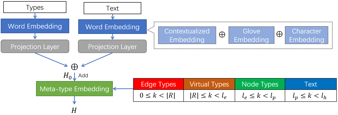
Figure 2: The encoder architecture of our model, where the $\oplus$ symbol is the concatenation operator, $k$ is the index of the word vectors in $H_{0}$, and $l_{e}=|R|+|U|$. The colored table on the right indicates the assignment of the meta-types for different blocks of the concatenated word vectors from $H_{0}$.

3 HySPA: Hybrid Span Generation for Alternating Sequences

In order to directly generate a target sequence that alternates between nodes that represent spans in the input and a set of node/edge types that depend on our extraction task, we first build a hybrid representation $H$ that is a concatenation of the hidden representations from edge types, node types and the input text. This representation functions as both the context space and the output space for our decoder. Then we invertibly map both the spans of input text and the indices of the types to the hybrid spans grounded on the representation $H$. Finally, hybrid spans are generated auto-regressively through a hybrid span decoder to form the alternating sequence $y^{\pi}\in S^{\pi}$. By translating the graph extraction task to a sequence generation task, we can easily use beam-search decoding to reduce possible exposure bias Wiseman and Rush (2016) of the sequential decision process and thus find globally better graph representation.

High-level overview of HySPA:

The HySPA model takes a piece of text (e.g. a sentence or passage), and the pre-defined node and edge types as input, and outputs an alternating sequence representation of an information graph. We enforce the generation of this sequence to be alternated by applying an alternating mask to the output probabilities. The detailed architecture is described in the following subsections.

3.1 Text and Types Encoder

Figure 2 shows the encoder architecture of our proposed model. For the set of node types, $Q$, and the set of edge types, $R$, and the virtual edge types, $U$, we arrange the type list, $\mathbf{v}$ as a concatenation of the label names of the edge types, virtual edge types and node types, i.e.,

$$\mathbf{v} =\hat{R}\oplus\hat{U}\oplus\hat{Q}$$

$$\hat{R} =[R_{1},...,R_{|R|}]$$

$$\hat{U} =[U_{1},...,U_{|U|}]$$

$$\hat{Q} =[Q_{1},...,Q_{|Q|}]$$

where $\oplus$ means the concatenation operator between two lists, and $\hat{R},\hat{U},\hat{Q}$ are the lists of the type names in the sets $R,U,Q$, respectively (e.g. $\hat{Q}=[\text{``Geopolitics''},\text{``Person''},...]$). Note that the concatenation order between the lists of type names can be arbitrary as long as it is kept consistent throughout the whole model. Then, as in the embedding part of the table-sequence encoder Wang and Lu (2020), for each type, $v_{i}$, we embed the label tokens of the types with the contextualized word embedding from a pre-trained language model, the GloVe embedding Pennington et al. (2014) and the character embedding,

$$E_{1} =\text{ContextualizedEmbed}(\mathbf{v}),\in R^{~{}l_{p}\times d_{c}}$$

$$E_{2} =\text{GloveEmbed}(\mathbf{v}),\in R^{~{}l_{p}\times d_{g}}$$

$$E_{3} =\text{CharacterEmbed}(\mathbf{v}),\in R^{~{}l_{p}\times d_{k}}$$

$$E_{4} =E_{1}\oplus E_{2}\oplus E_{3}\in R^{~{}l_{p}\times d_{e}},$$

$$E_{v} =E_{4}W_{0}^{T}\in R^{~{}l_{p}\times d_{m}},$$

where $l_{p}=|R|+|U|+|Q|$ is the number of all kinds of types, $W_{0}\in R^{~{}d_{e}\times d_{m}}$ is the weight matrix of the linear projection layer, $d_{e}=d_{c}+d_{g}+d_{k}$ is the total embedding dimension and $d_{m}$ is the hidden size of our model. After we obtain the contextualized embedding of the tokens of each type $v_{i}\in\mathbf{v}$, we take the average of these token vectors as the representation of $v_{i}$ and freeze its update during training. More details of the embedding pipeline can be found in Appendix A.

This embedding pipeline is also used to embed the words in the input text, $\mathbf{x}$. Unlike the pipeline for the type embedding, we represent the word as the contextualized embedding of its first sub-token from the pre-trained Language Model (LM, e.g. BERT Devlin et al. (2018)), and finetune the LM in an end-to-end fashion.

After obtaining the type embedding $E_{v}$, and the text embedding $E_{x}$ respectively, we concatenate them along the sequence length dimension to form the hybrid representation $H_{0}$. Since $H_{0}$ is a concatenation of word vectors from four different types of tokens, i.e., edge types, virtual edge types, node types and text, a meta-type embedding is applied to indicate this type difference between the blocks of vectors from the representation $H_{0}$, as shown in Figure 2. The final context representation $H$ is obtained by element-wise addition of the meta-type embedding and $H_{0}$,

$$H_{0} =E_{v}\oplus E_{x}\in R^{l_{h}\times d_{m}},$$

$$H_{s} =\text{MetaTypeEmbed}(H_{0})\in R^{l_{h}\times d_{m}},$$

$$H =H_{0}+H_{s}\in R^{l_{h}\times d_{m}},$$

where $l_{h}=l_{p}+|x|$ is the height of our hybrid representation matrix $H$.

3.2 Invertible Mapping between Spans & Types and Hybrid Spans

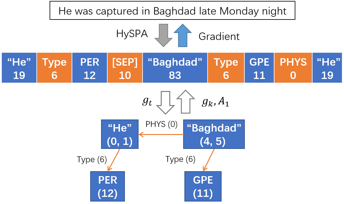
Figure 3: An example of the alternating sequence representation (in the middle) of a knowledge graph (at bottom) from the ACE05 training set, where $A_{1}$ means the Algorithm 1. We take $m=16$ and $l_{p}=19$ for this example. “19” in the alternating sequence is the index for the span (0,1) of “He”, “83” is the index for the span (4,5) of “Baghdad”, and “10” is the index of the virtual edge type, [SEP]. The input text (on top) for this graph is “He was captured in Baghdad late Monday night”.

Given a span in the text, $t=(t_{s},t_{e})\in\mathbb{N}^{2},t_{s}<t_{e}$, we convert the span $t$ to an index $k$, $k\geq l_{p}$, in the representation $H$ via the mapping $g_{k}$,

$$k=g_{k}(t_{s},t_{e})=t_{s}m+t_{e}-t_{s}-1+l_{p}\in\mathbb{N},$$

where $m$ is the maximum length of spans, and $l_{p}=|R|+|U|+|Q|$. We keep the type indices in the graph unchanged because they are smaller than $l_{p}$ and $k\geq l_{p}$. Since, for an information graph, the maximum span length, $m$, of a mention is often far smaller than the length of the text, i.e., $m\ll n$, we can then reduce the bound of the maximum magnitude of $k$ from $O(n^{2})$ to $O(nm)$ by only considering spans of length smaller than $m$, and thus maintain linear space complexity for our decoder with respect to the length of the input text, $n$. Figure 3 shows a concrete example of our alternating sequence for a knowledge graph in the ACE05 dataset.

Since $t_{s},t_{e},k$ are all natural numbers, we can construct an inverse mapping $g_{t}$ that converts the index $k$ in $H$ back to $t=(t_{s},t_{e})$,

$$t_{s}=g_{t_{s}}(k)=-\text{max} (0,-k+l_{p})+$$

$$\lfloor\text{max}(0,k-l_{p})/m\rfloor+l_{p},$$

$$t_{e}=g_{t_{e}}(k)=g_{t_{s}}(k) +\text{max}(0,k-l_{p})~{}\text{mod}~{}m,$$

where $\lfloor\cdot\rfloor$ is the integer floor function and $\mod$ is the modulus operator. Note that $g_{t}(k)$ can be directly applied to the indices from the types segment of $H$ and remain their values unchanged, i.e.,

$$g_{t}(k)=(k,k),\forall k<l_{p},k\in\mathbb{N}.$$

With this property, we can easily incorporate the mapping $g_{t}$ into our decoder to map the alternating sequence $y^{\pi}$ back to the spans in the hybrid representation $H$.

3.3 Hybrid Span Decoder

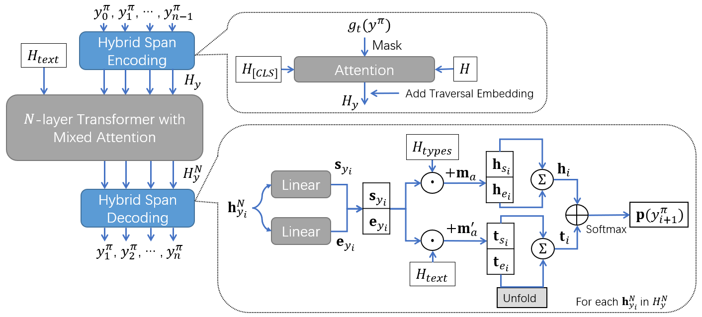
Figure 4: The architecture of our hybrid span decoder. $N$ is the number of the decoder layers. $\oplus$ before the softmax function means the concatenation operator. $H_{y}^{N}$ is the hidden representation of the sequence $y^{\pi}$ from the last decoder layer. Our hybrid span decoder can be understood as an auto-regressive model that operates in a closed context space and output space defined by $H$.

Figure 4 shows the general model architecture of our hybrid span decoder. Our decoder takes the context representation $H$ as input, and recurrently decodes the alternating sequence $y^{\pi}$ given a start-of-sequence token.

Figure 5: An example of BFS traversal embedding for an alternating sequence, [“He”, Type, PER, [SEP], “Baghdad”, Type, GPE, PHYS, “He”]. Our traversal embedding is the sum of the level embedding, the parent-child embedding and the tree embedding.

Hybrid Span Encoding via Attention

Given the alternating sequence $y^{\pi}$, and the mapping $g_{t}$ (section 3.2), our decoder first maps each index in $y^{\pi}$ to a span, $(t_{s_{i}},t_{e_{i}})=g_{t}(y_{i}^{\pi})$, grounded on the representation $H$ and then converts the span to an attention mask, $M_{0}$, to allow the model to learn to represent a span as a weighted sum of a segment of the contextualized word representations referred by the span,

$$Q =W_{1}^{T}H_{[CLS]}+\mathbf{b}_{1}\quad\in R^{~{}|y^{\pi}|\times d_{m}},$$

$$K =W_{2}^{T}H+\mathbf{b}_{2}\quad\in R^{~{}l_{h}\times d_{m}},$$

$$H_{y} =\text{softmax}\bigg{(}\frac{QK^{T}}{\sqrt{d_{m}}}+M_{0}\bigg{)}H\quad\in R^{~{}|y^{\pi}|\times d_{m}},$$

$$M_{0} (i,j)=\left\{\begin{array}[]{c l}0,&t_{s_{i}}\leq j\leq t_{e_{i}}\\ -\infty,&\text{otherwise}\end{array}\right.$$

where $H_{[CLS]}\in R^{~{}|y^{\pi}|\times d_{m}}$ is the $|y^{\pi}|$-times repeated hidden representation of the start of the sequence token, [CLS], from the text segment of $H$, and $H_{y}$ is our final representation of the hybrid spans in $y^{\pi}$. $W_{1},W_{2},\mathbf{b}_{1},\mathbf{b}_{2}$ are learnable parameters, and $t_{s_{i}},t_{e_{i}}$ are the start and the end position of the span thatwe are encoding. Note that for the type spans whose length is 1, the result of the softmax calculation will always be 1, which leads to its span representation to be exactly its embedding vector as we desired.

Traversal Embedding

In order to distinguish the hybrid spans at different position in $y^{\pi}$, a naive way is to add a sinusoidal position embedding Vaswani et al. (2017) to $H_{y}$. However, this approach treats the alternating sequence as an ordinary sequence and ignores the underlying graph structure it encodes. To alleviate this issue, we propose a novel traversal embedding approach which captures the traversal level information, the parent-child information and the intra-level connection information as a substitution of the naive position embedding. Our traversal embedding can either encode the BFS or DFS traversal pattern. As an example, we assume BFS traversal here and leave the details of DFS traversal embedding in Appendix D.

Our BFS traversal embedding is a pointwise sum of the level embedding, $L$, the parent-child embedding, $P$, and the tree embedding, $T$ of a given alternating sequence, $y$,

$$\text{TravEmbed}(y)=L(y)+P(y)+T(y)\in R^{~{}|y|\times d_{m}}$$

where the level embedding assigns the same embedding vector $L_{i}$ for each position at the BFS traversal level $i$, and the value of the embedding vector is filled according to the non-parametric sinusoidal position embedding since we want our embedding to extrapolate to the sequence that is longer than any sequences in the training set. The parent-child embedding assigns different random initialized embedding vectors at the positions of the parent nodes and the child nodes in the BFS traversal levels to help model distinguish between these two kinds of nodes. For encoding the intra-level connection information, our insight is that the connection between each nodes in a BFS level can be viewed as a depth-3 tree, where the first depth takes the parent node, the second depth is filled with the edge types and the third depth consists of the corresponding child nodes for each of the edge types. Our tree embedding is then formed by encoding the position information of the depth-3 tree with a tree positional embedding Shiv and Quirk (2019) for each BFS level. Figure 5 shows a concrete example of how these embeddings function for a given alternating sequence. The obtained traversal embedding is then pointwisely added to the hidden representation of the alternating sequence $H_{y}$ for injecting the traversal information of the graph structure.

Inner blocks

With the input text representation $H_{text}$ sliced from the hybrid representation $H$ and the target sequence representation $H_{y}$, we apply an $N$-layer transformer structure with mixed-attention He et al. (2018) to allow our model to utilize features from different attention layers when decoding the edges or the nodes of an alternating sequence. Note that our hybrid span decoder is perpendicular to the actual choice of the neural structures of the inner blocks, and we choose the design of mixed-attention transformer He et al. (2018) because its layerwise coordination property is empirically more suitable for our heterogeneous decoding of two different kinds of sequence elements. The detailed structure of the inner blocks is explained in Appendix E.

Hybrid span decoding

For the hybrid span decoding module, we first slice off the hidden representation of the alternating sequence $y^{\pi}$ from the output of the $N$-layer inner blocks and denote it as $H_{y}^{N}$. Then for each hidden representation $\mathbf{h}_{y_{i}}^{N}\in H_{y}^{N},0\leq i<|y^{\pi}|$, we apply two different linear layers to obtain the start position representation, $\mathbf{s}_{y_{i}}$, and the end position representation, $\mathbf{e}_{y_{i}}$,

$$\mathbf{s}_{y_{i}} =W_{5}^{T}\mathbf{h}_{y_{i}}+\mathbf{b}_{5}\quad\in R^{~{}d_{m}},$$

$$\mathbf{e}_{y_{i}} =W_{6}^{T}\mathbf{h}_{y_{i}}+\mathbf{b}_{6}\quad\in R^{~{}d_{m}},$$

where $W_{5},W_{6}\in R^{~{}d_{m}\times d_{m}}$ and $\mathbf{b}_{5},\mathbf{b}_{6}\in R^{~{}d_{m}}$ are learnable parameters. Then we calculate the scores of the target spans separately for the types segment and the text segment of $H$, and concatenate them together before the final softmax operator for a joint estimation of the probabilities of text spans and type spans,

$$\mathbf{h}_{s_{i}} =H_{\text{types}}~{}\mathbf{s}_{y_{i}}+\mathbf{m}_{a} \in R^{l_{p}},$$

$$\mathbf{h}_{e_{i}} =H_{\text{types}}~{}\mathbf{e}_{y_{i}}+\mathbf{m}_{a} \in R^{l_{p}},$$

$$\mathbf{h}_{i} =\mathbf{h}_{s_{i}}+\mathbf{h}_{e_{i}} \in R^{l_{p}},$$

$$\mathbf{t}_{s_{i}} =H_{\text{text}}~{}\mathbf{s}_{y_{i}}+\mathbf{m}_{a}^{\prime} \in R^{n},$$

$$\mathbf{t}_{e_{i}} =H_{\text{text}}~{}\mathbf{e}_{y_{i}}+\mathbf{m}_{a}^{\prime} \in R^{n},$$

$$\mathbf{t}_{i} =\text{unfold}(\mathbf{t}_{e_{i}},m)+\mathbf{t}_{s_{i}} \in R^{nm},$$

$$\mathbf{p}(y_{i+1}^{\pi}) =\text{softmax}(\mathbf{h}_{i}\oplus\mathbf{t}_{i}) \in R^{nm+l_{p}},$$

where $\mathbf{h}_{i}$ is the score vector of possible spans in the type segment of $H$, and $\mathbf{t}_{i}$ is the score vector of possible spans in the text segment of $H$. Since the type spans always have a span length 1, we only need an element-wise addition between the start position scores, $\mathbf{h}_{s_{i}}$ and the end position scores $\mathbf{h}_{e_{i}}$ to calculate $\mathbf{h}_{i}$. The entries of $\mathbf{t}_{i}$ contain the scores for the text spans, $t_{s_{i},j}+t_{e_{i},k},\forall j\leq k,k-j<m$, which are calculated with the help of an unfold function which converts the vector $\mathbf{t}_{e_{i}}\in R^{n}$ to a stack of $n$ sliding windows of size $m$, the maximum span length, with stride 1. The alternating masks $\mathbf{m}_{a}\in R^{l_{p}},\mathbf{m}_{a}^{\prime}\in R^{n}$ are defined as:

$$\mathbf{m}_{a}(j)= \left\{\begin{array}[]{c l}0,&y_{i}^{\pi}>l_{e}\cap j<l_{e}\\ -\infty,&\text{otherwise}\end{array}\right.$$

$$\mathbf{m}_{a}^{\prime}(j)= \left\{\begin{array}[]{c l}-\infty,&y_{i}^{\pi}>l_{e}\\ 0,&\text{otherwise}\end{array}\right.$$

where $l_{e}=|R|+|U|$ is the total number of edge types. In this way, while we have a joint model of nodes and edge types, the output distribution is enforced by the alternating masks to produce an alternating decoding of nodes and edge types, and this is the main reason why we call this decoder a hybrid span decoder.

IE Models	Space Complexity	Time Complexity	NER	RE
PointerNet Katiyar and Cardie (2017)	$O(n)$	$O(n^{2})$	82.6	55.9
SpanRE Dixit and Al-Onaizan (2019)	$O(n)$	$O(n^{2})$	86.0	62.8
Dygie++ Wadden et al. (2019)	$O(n)$	$O(n^{2})$	88.6	63.4
OneIE Lin et al. (2020)	$O(n)$	$O(n^{2})$	88.8	67.5
TabSeq Wang and Lu (2020)	$O(n^{2})$	$O(n)$	89.5	67.6
HySPA (ours)  w/ RoBERTa	$O(n)$	$O(n)$	88.9	68.2
w/ ALBERT			89.9	68.0

Table 1: Joint NER and RE F1 scores of the IE models on the ACE05 test set. Complexities are calculated for the entity and relation decoding part of the models ($n$ is the length of the input text). The performance of the TabSeq model reported here is based on the same ALBERT-xxlarge Lan et al. (2020) pretrained language model as ours.

4 Experiments

4.1 Experimental Setting

We test our model on the ACE 2005 dataset distributed by LDC, which includes 14.5k sentences, 38.3k entities (with 7 types), and 7.1k relations (with 6 types), derived from the general news domain. More details can be found in Appendix C.

Following previous work, we use F1 as an evaluation metric for both NER and RE. For the NER task, a prediction is marked correct when both the type and the boundary span match those of the gold entity. For the RE task, a prediction is correct when both the relation type and the boundaries of the two entities are correct.

4.2 Implementation Details

When training our model, we apply the cross-entropy loss with a label smoothing factor of 0.1. The model is trained with 2048 tokens per batch (roughly a batch size of 28) for 25000 steps using an AdamW optimizer Loshchilov and Hutter (2018) with a learning rate of $2e^{-4}$, a weight decay of 0.01, and an inverse square root scheduler with 2000 warm-up steps. Following the TabSeq model Wang and Lu (2020), we use RoBERTa-large Liu et al. (2019) or ALBERT-xxlarge-v1 Lan et al. (2020) for the pretrained language model and slow its learning rate by a factor of 0.1 during training. A hidden state dropout rate of 0.2 is applied to RoBERTa-large while the rate of 0.1 for ALBERT-xxlarge-v1. A dropout rate of 0.1 is also applied to our hybrid span decoder during training. We set the maximum span length, $m=16$, the hidden size of our model, $d_{m}=256$, and the number of the decoder blocks, $N=12$. Even though theoretically the beam-search should help us reduce the exposure bias, we do not observe any performance gain during grid search of the beam size and the length penalty on the validation set (detailed grid search setting is in Appendix A). Thus we set a vanilla beam size of 1 and the length penalty of 1, and leave this theory-experiment contradiction for future research. Our model is built with the FAIRSEQ toolkit Ott et al. (2019) for efficient distributed training and all the experiments are conducted on two NVIDIA TITAN X GPUs.

4.3 Results

Table 1 compares our model with the previous state-of-the-art results on the ACE05 test set. Compared with the previous SOTA, TabSeq Wang and Lu (2020) with ALBERT pretrained language model, our model with ALBERT has significantly better performance for both NER score and RE score, while maintaining a linear space complexity which is an order smaller than TabSeq. Our model is the first joint model that has both linear space and time complexities compared with all previous joint IE models, and thus has the best scalability for large-scale real world applications.

4.4 Ablation Study

Model	NER F1	RE F1
HySPA w/ RoBERTa	88.9	68.2
– Traversal-embedding	88.9	66.7
– Masking	88.1	64.8
– BFS	88.7	66.2
– Mixed-attention	88.6	64.7
– Span-attention	88.5	66.1

Table 2: Ablation study on the ACE05 test set. “– Traversal-embedding”: we remove the traversal embedding and instead use sinusoidal position embedding, and the following ablations are based on the model after this ablation. “– Masking”: we remove the alternating mask from the hybrid span decoder. “– BFS”: we use DFS instead of BFS as traversal. “– Mixed-attention”: we remove the mixed-attention layer and use a standard transformer encoder decoder structure. “– Span-attention”: we remove the span attention in the span encoding module and instead average the words in the span.

To prove the effectiveness of our approach, we conduct ablation experiments on the ACE05 dataset. As shown in Table 2, after we remove the traversal embedding the RE F1 scores drop significantly, which indicates that our traversal embedding can help encode the graph structure and improve relation predictions. Also if the alternating masking is dropped, the NER F1 and RE F1 scores both drop significantly, which proves the importance of enforcing the alternating pattern. We can observe that the mixed-attention layer contributes significantly for relation extraction. This is because the layer-wise coordination can help the decoder to disentangle the source features and utilize different layer features between the entity and the relation prediction. We can also observe that the DFS traversal has worse performance than BFS. We suspect that this is because the resultant alternating sequence from DFS is often longer than the one from BFS due to the nature of the knowledge graphs, and thus increases the learning difficulty.

4.5 Error Analysis

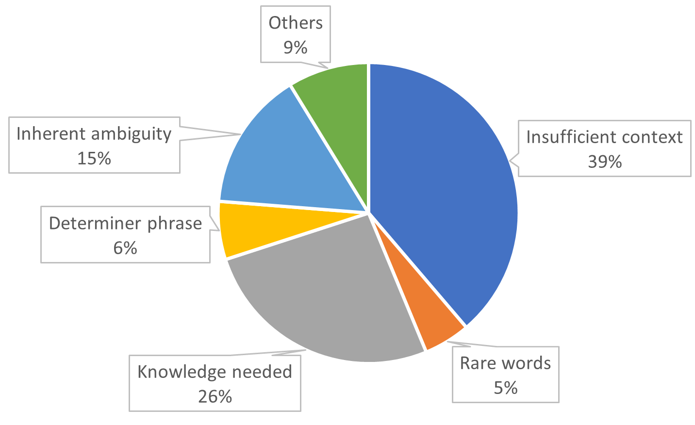
Figure 6: Distribution of remaining errors on the ACE05 test set.

After analyzing 80 remaining errors, we categorize and discuss common cases below (Figure 6 plots the distribution of error types). These may require additional features and strategies to address.

Insufficient context. In many examples, the answer entity is a pronoun that cannot be accurately typed given the limited context: in “We notice they said they did not want to use the word destroyed, in fact, they said let others do that”, it’s difficult to correctly classify We as an organization. This could be mitigated by using entire documents as input, leveraging cross-sentence context.

Rare words. The rare word issue is when the word in test set rarely appeared in the training set and often not termed in the dictionary. In the sentence “There are also Marine FA-18s and Marine Heriers at this base”, the term Heriers (a vehicle incorrectly classified as person by the model) neither appeared in the training set, nor understood well by pre-trained language model; the model, in this case, can only rely on subword-level representation.

Background knowledge required Often the sentence mentions entities that are difficult to infer from the context, but are easily identified by consulting a knowledge base: in “but critics say Airbus should have sounded a stronger alarm after a similar incident occurred in 1997”, our model incorrectly predicts the Airbus to be a vehicle while the Airbus here refers to the European aerospace corporation. Our system also separated United Nations Security Council into two entities United Nations and Security Council, generating a non-existing relation triple (Security Council part-of United Nations). Such mistakes could be avoided by consulting a knowledge base such as DBpedia Bizer et al. (2009) or by performing entity linking.

Inherent ambiguity Many examples have inherent ambiguity, e.g. European Union can be typed as organization or political entity, while some entities (e.g., military bases) can be both locations and organizations, or facilities.

5 Related Work

NER is often done jointly with RE in order to mitigate error propagation and learn inter-relation between tasks. One line of approaches is to treat the joint task as a squared table filling problem Miwa and Sasaki (2014); Gupta et al. (2016); Wang and Lu (2020), where the $i$-th column or row represents the $i$-th token. The table has diagonals indicating sequential tags for entities and other entries as relations between pairs of tokens. Another line of work is by performing RE after NER. In the work by Miwa and Bansal (2016), the authors used BiLSTM Graves et al. (2013) for NER and consequently a Tree-LSTM Tai et al. (2015) based on dependency graph for RE. Wadden et al. (2019) and Luan et al. (2019), on the other hand, takes the approach of constructing dynamic text span graphs to detect entities and relations. Extending on Wadden et al. (2019), Lin et al. (2020) introduced OneIE, which further incorporates global features based on cross subtask and instance constraints, aiming to extract IE results as a graph. Note that our model differs from OneIE Lin et al. (2020) in that our model captures global relationships automatically through autoregressive generation while OneIE uses feature engineered templates; Moreover, OneIE needs to do pairwise classification for relation extraction, while our method efficiently generates existing relations and entities.

While several Seq2Seq-based models Zhang et al. (2020); Zeng et al. (2018, 2020); Wei et al. (2019); Zhang et al. (2019) have been proposed to generate triples (i.e., node-edge-node), our model is fundamentally different from them in that: (1) it is generating a BFS/DFS traversal of the target graph, which captures dependencies between nodes and edges and has a shorter target sequence, (2) we model the nodes as the spans in the text, which is independent of the vocabulary, so even if the tokens of the nodes are rare or unseen words, we can still generate spans on them based on the context information.

6 Conclusion

In this work, we propose the Hybrid Span Generation (HySPA) model, the first end-to-end text-to-graph extraction model that has a linear space and time complexity at the graph decoding stage. Besides its scalability, the model also achieves state-of-the-art performance on the ACE05 joint entity and relation extraction task. Given the flexibility of the structure of our hybrid span generator, abundant future research directions remain, e.g. incorporating the external knowledge for hybrid span generation, applying more efficient sparse self-attention, and developing better search methods to find more globally plausible graphs represented by the alternating sequence.

Appendix A Hyperparameters

We use 100-dimensional GloVe word embeddings trained on 6B tokens as intialization , and freeze its update during training. The character embedding has 30-dimension with LSTM encoding and the Glove Embeddings for the out of vocabulary tokens are replaced with randomly initialized vectors following Wang and Lu (2020). We use gradient clipping of 0.25 during training. The number of heads for our mixed attention is set to 8. The beam size and length penalty is decided by a grid-search on the validation set of the ACE05 dataset, and the range for the beam size is from 1 to 7 with a step size of 1 and the length penalty is from 0.7 to 1.2 with a step size of 0.1. We choose the best beam size and length penalty based on the metric of relation extraction F1 score.

Appendix B Training Details

Our model has 236 million parameters with the ALBERT-xxlarge pretrained language model. On average, our best performing model with ALBERT-xxlarge can be trained distributedly on two NVIDIA TITAN X GPUs for 20 hours.

Appendix C Data

The Automatic Content Extraction (ACE) 2005  dataset contains English, Arabic and Chinese training data for the 2005 Automatic Content Extraction (ACE) technology evaluation, providing entity, relation, and event annotations. We follow Wadden et al. (2019)  for preprocessing and data splits. The preprocessed data contains 7.1k relations, 38k entities, and 14.5k sentences. The split contains 10051 samples for training, 2424 samples for development, and 2050 for testing.

Appendix D DFS Traversal Embedding

Since the parent-child information is already contained in the intra-level connections of DFS traversal, we only have the sum of the level embedding and the connection embedding for DFS traversal embedding. Similar to BFS embedding, the DFS level embedding assigns the same embedding vector $L_{i}$ for each position at the DFS traversal level $i$, but the value of the embedding vector is randomly initialized instead of filled with the non-parametric sinusoidal position embedding, since the proximity information does not exist between the traversal levels of DFS. However, we do have clear distance information for the elements in a DFS level, i,e., for a DFS level $D=[\text{A, B, C, ..., [sep]}]$, the distance from A to the elements [A, B, C, …, [sep]] is $[0,1,2,3,...,|D|-1]$. We encode this distance information with the sinusoidal position embedding which becomes our connection embedding that captures the intra-level connection information.

Appendix E Transformer with Mixed-attention

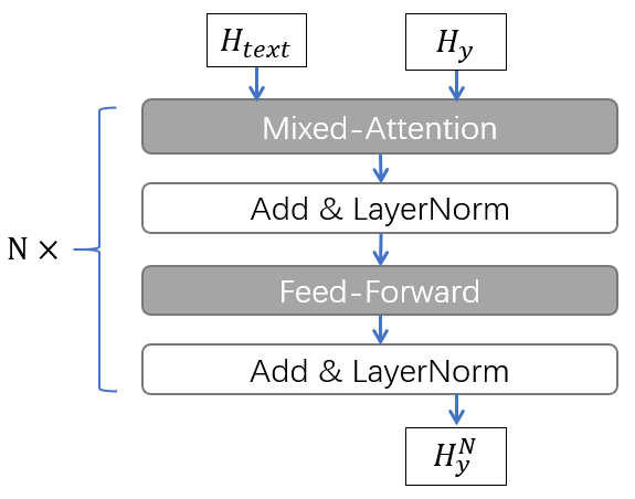
Figure 7: The general model architecture of the mixed-attention transformer.

We first slice off the hidden representation of the input text from the hybrid representation $H$, and denote it as $H_{\text{text}}$, then the input text representation $H_{\text{text}}$ and the output from the Hybrid Span Encoding $H_{y}$ gets fed into a stack of $N$ mixed-attention/feedforward blocks that have the following structure (as shown in Figure 7):

Since generating the node and edge types may need features from different layers, we use mixed attention He et al. (2018), which allows our model to utilize the features from different attention layers when encoding the text segment, $H_{text}$, and the target features, $H_{y}$,

$$\text{MixedAtt}(Q,K,V) =\text{softmax}\bigg{(}\frac{QK^{T}}{\sqrt{d_{m}}}+M_{1}\bigg{)}V$$

$$\quad\quad\in R^{~{}l_{m}\times d_{m}},$$

$$M_{1}(i,j)= \left\{\begin{array}[]{c l}0,&j<n\cup j\leq i+n\\ -\infty,&\text{otherwise}\end{array}\right.$$

where $n=|x|$ is the length of the input text, $l_{m}=|x|+|y^{\pi}|$ is the total length of the source and the target features. Denoting the concatenation of the source features, $H_{\text{text}}$, and the target features, $H_{y}$, as $H_{0}$, a source/target embedding He et al. (2018) is also added to $H_{0}$ before the first layer of the mixed attention to allow the model to distinguish the features from the source and the target sequences. The mixed-attention layer is combined with a feed-forward layer to form a decoder block:

FFN $$(x)=\text{max}(0,xW_{3}+b_{3})W_{4}+b_{4},$$

$$Q=W_{q}^{T}H_{0}+\mathbf{b}_{q},$$

$$K=W_{k}^{T}H_{0}+\mathbf{b}_{k},$$

$$V=W_{v}^{T}H_{0}+\mathbf{b}_{v},$$

$$H_{0}^{\prime} =\text{LayerNorm}(\text{MixedAtt}(Q,K,V)+H_{0}),$$

$$H_{1} =\text{LayerNorm}(\text{FFN}(H_{0}^{\prime})+H_{0}^{\prime}),$$

where $W_{q,k,v},\mathbf{b}_{q,k,v},W_{3}\in R^{~{}d_{m}\times 4d_{m}},W_{4}\in R^{~{}4d_{m}\times d_{m}},\mathbf{b}_{3},\mathbf{b}_{4}$ are the learnable parameters, and LayerNorm is the Layer Normalization layer Ba et al. (2016). The decoder block is stacked $N$ times to obtain the final hidden representation $H_{N}$, and output the final representation of the target sequence, $H_{y}^{N}$. The mixed-attention has a time complexity of $O(n^{2})$ when encoding the source features, but we can cache the hidden representation of this part when generating the target tokens due to the causal masking of the target features, and thus maintain a time complexity of $O(n)$ for each decoding step.

References

- Ba et al. (2016) Jimmy Ba, J. Kiros, and Geoffrey E. Hinton. 2016. Layer normalization. ArXiv, abs/1607.06450.
- Bizer et al. (2009) Christian Bizer, Jens Lehmann, Georgi Kobilarov, Sören Auer, Christian Becker, Richard Cyganiak, and Sebastian Hellmann. 2009. Dbpedia-a crystallization point for the web of data. Journal of web semantics, 7(3):154–165.
- Chan and Roth (2011) Yee Seng Chan and Dan Roth. 2011. Exploiting syntactico-semantic structures for relation extraction. In Proceedings of the 49th Annual Meeting of the Association for Computational Linguistics: Human Language Technologies, pages 551–560, Portland, Oregon, USA. Association for Computational Linguistics.
- Cho et al. (2014) Kyunghyun Cho, Bart van Merriënboer, Caglar Gulcehre, Dzmitry Bahdanau, Fethi Bougares, Holger Schwenk, and Yoshua Bengio. 2014. Learning phrase representations using RNN encoder–decoder for statistical machine translation. In Proceedings of the 2014 Conference on Empirical Methods in Natural Language Processing (EMNLP), pages 1724–1734, Doha, Qatar. Association for Computational Linguistics.
- Devlin et al. (2018) Jacob Devlin, Ming-Wei Chang, Kenton Lee, and Kristina Toutanova. 2018. Bert: Pre-training of deep bidirectional transformers for language understanding. arXiv preprint arXiv:1810.04805.
- Dixit and Al-Onaizan (2019) Kalpit Dixit and Yaser Al-Onaizan. 2019. Span-level model for relation extraction. In Proceedings of the 57th Annual Meeting of the Association for Computational Linguistics, pages 5308–5314, Florence, Italy. Association for Computational Linguistics.
- Eberts and Ulges (2019) Markus Eberts and Adrian Ulges. 2019. Span-based joint entity and relation extraction with transformer pre-training. arXiv preprint arXiv:1909.07755.
- Florian et al. (2006) Radu Florian, Hongyan Jing, Nanda Kambhatla, and Imed Zitouni. 2006. Factorizing complex models: A case study in mention detection. In Proceedings of the 21st International Conference on Computational Linguistics and 44th Annual Meeting of the Association for Computational Linguistics, pages 473–480, Sydney, Australia. Association for Computational Linguistics.
- Florian et al. (2010) Radu Florian, John Pitrelli, Salim Roukos, and Imed Zitouni. 2010. Improving mention detection robustness to noisy input. In Proceedings of the 2010 Conference on Empirical Methods in Natural Language Processing, pages 335–345, Cambridge, MA. Association for Computational Linguistics.
- Graves et al. (2007) Alex Graves, Santiago Fernández, and Jürgen Schmidhuber. 2007. Multi-dimensional recurrent neural networks. In International conference on artificial neural networks, pages 549–558. Springer.
- Graves et al. (2013) Alex Graves, Abdel-rahman Mohamed, and Geoffrey Hinton. 2013. Speech recognition with deep recurrent neural networks. In 2013 IEEE international conference on acoustics, speech and signal processing, pages 6645–6649. Ieee.
- Gupta et al. (2016) Pankaj Gupta, Hinrich Schütze, and Bernt Andrassy. 2016. Table filling multi-task recurrent neural network for joint entity and relation extraction. In Proceedings of COLING 2016, the 26th International Conference on Computational Linguistics: Technical Papers, pages 2537–2547.
- He et al. (2018) Tianyu He, Xu Tan, Yingce Xia, Di He, Tao Qin, Zhibo Chen, and Tie-Yan Liu. 2018. Layer-wise coordination between encoder and decoder for neural machine translation. In Advances in Neural Information Processing Systems, volume 31, pages 7944–7954. Curran Associates, Inc.
- Jiang and Zhai (2007) Jing Jiang and ChengXiang Zhai. 2007. A systematic exploration of the feature space for relation extraction. In Human Language Technologies 2007: The Conference of the North American Chapter of the Association for Computational Linguistics; Proceedings of the Main Conference, pages 113–120, Rochester, New York. Association for Computational Linguistics.
- Katiyar and Cardie (2017) Arzoo Katiyar and Claire Cardie. 2017. Going out on a limb: Joint extraction of entity mentions and relations without dependency trees. In Proceedings of the 55th Annual Meeting of the Association for Computational Linguistics (Volume 1: Long Papers), pages 917–928, Vancouver, Canada. Association for Computational Linguistics.
- Kolluru et al. (2020) Keshav Kolluru, Samarth Aggarwal, Vipul Rathore, Soumen Chakrabarti, et al. 2020. Imojie: Iterative memory-based joint open information extraction. arXiv preprint arXiv:2005.08178.
- Lan et al. (2020) Zhenzhong Lan, Mingda Chen, Sebastian Goodman, Kevin Gimpel, Piyush Sharma, and Radu Soricut. 2020. Albert: A lite bert for self-supervised learning of language representations. In International Conference on Learning Representations.
- Li and Ji (2014) Qi Li and Heng Ji. 2014. Incremental joint extraction of entity mentions and relations. In Proceedings of the 52nd Annual Meeting of the Association for Computational Linguistics (Volume 1: Long Papers), pages 402–412, Baltimore, Maryland. Association for Computational Linguistics.
- Li et al. (2014) Qi Li, Heng Ji, Yu Hong, and Sujian Li. 2014. Constructing information networks using one single model. In Proceedings of the 2014 Conference on Empirical Methods in Natural Language Processing (EMNLP), pages 1846–1851, Doha, Qatar. Association for Computational Linguistics.
- Lin et al. (2020) Ying Lin, Heng Ji, Fei Huang, and Lingfei Wu. 2020. A joint neural model for information extraction with global features. In Proceedings of the 58th Annual Meeting of the Association for Computational Linguistics, pages 7999–8009, Online. Association for Computational Linguistics.
- Liu et al. (2019) Y Liu, M Ott, N Goyal, J Du, M Joshi, D Chen, O Levy, M Lewis, L Zettlemoyer, and V Stoyanov. 2019. Roberta: A robustly optimized bert pretraining approach. arxiv 2019. arXiv preprint arXiv:1907.11692.
- Liu et al. (2018) Yue Liu, Tongtao Zhang, Zhicheng Liang, Heng Ji, and Deborah L McGuinness. 2018. Seq2rdf: An end-to-end application for deriving triples from natural language text. arXiv preprint arXiv:1807.01763.
- Loshchilov and Hutter (2018) Ilya Loshchilov and Frank Hutter. 2018. Decoupled weight decay regularization. In International Conference on Learning Representations.
- Luan et al. (2019) Yi Luan, Dave Wadden, Luheng He, Amy Shah, Mari Ostendorf, and Hannaneh Hajishirzi. 2019. A general framework for information extraction using dynamic span graphs. arXiv preprint arXiv:1904.03296.
- Miwa and Bansal (2016) Makoto Miwa and Mohit Bansal. 2016. End-to-end relation extraction using lstms on sequences and tree structures. arXiv preprint arXiv:1601.00770.
- Miwa and Sasaki (2014) Makoto Miwa and Yutaka Sasaki. 2014. Modeling joint entity and relation extraction with table representation. In Proceedings of the 2014 Conference on Empirical Methods in Natural Language Processing (EMNLP), pages 1858–1869.
- Ott et al. (2019) Myle Ott, Sergey Edunov, Alexei Baevski, Angela Fan, Sam Gross, Nathan Ng, David Grangier, and Michael Auli. 2019. fairseq: A fast, extensible toolkit for sequence modeling. In Proceedings of NAACL-HLT 2019: Demonstrations.
- Pennington et al. (2014) Jeffrey Pennington, Richard Socher, and Christopher Manning. 2014. GloVe: Global vectors for word representation. In Proceedings of the 2014 Conference on Empirical Methods in Natural Language Processing (EMNLP), pages 1532–1543, Doha, Qatar. Association for Computational Linguistics.
- Shi et al. (2017) C. Shi, Y. Li, J. Zhang, Y. Sun, and P. S. Yu. 2017. A survey of heterogeneous information network analysis. IEEE Transactions on Knowledge and Data Engineering, 29(1):17–37.
- Shiv and Quirk (2019) Vighnesh Shiv and Chris Quirk. 2019. Novel positional encodings to enable tree-based transformers. In Advances in Neural Information Processing Systems, volume 32. Curran Associates, Inc.
- Sun et al. (2011) Ang Sun, Ralph Grishman, and Satoshi Sekine. 2011. Semi-supervised relation extraction with large-scale word clustering. In Proceedings of the 49th Annual Meeting of the Association for Computational Linguistics: Human Language Technologies, pages 521–529, Portland, Oregon, USA. Association for Computational Linguistics.
- Tai et al. (2015) Kai Sheng Tai, Richard Socher, and Christopher D Manning. 2015. Improved semantic representations from tree-structured long short-term memory networks. arXiv preprint arXiv:1503.00075.
- Vaswani et al. (2017) Ashish Vaswani, Noam Shazeer, Niki Parmar, Jakob Uszkoreit, Llion Jones, Aidan N Gomez, Łukasz Kaiser, and Illia Polosukhin. 2017. Attention is all you need. In Advances in neural information processing systems, pages 5998–6008.
- Wadden et al. (2019) David Wadden, Ulme Wennberg, Yi Luan, and Hannaneh Hajishirzi. 2019. Entity, relation, and event extraction with contextualized span representations. arXiv preprint arXiv:1909.03546.
- Wang and Lu (2020) Jue Wang and Wei Lu. 2020. Two are better than one: Joint entity and relation extraction with table-sequence encoders. arXiv preprint arXiv:2010.03851.
- Wei et al. (2019) Zhepei Wei, Jianlin Su, Yue Wang, Yuan Tian, and Yi Chang. 2019. A novel cascade binary tagging framework for relational triple extraction. arXiv preprint arXiv:1909.03227.
- Wiseman and Rush (2016) Sam Wiseman and Alexander M Rush. 2016. Sequence-to-sequence learning as beam-search optimization. In Proceedings of the 2016 Conference on Empirical Methods in Natural Language Processing, pages 1296–1306.
- Zeng et al. (2020) Daojian Zeng, Haoran Zhang, and Qianying Liu. 2020. Copymtl: Copy mechanism for joint extraction of entities and relations with multi-task learning. In Proceedings of the AAAI Conference on Artificial Intelligence, volume 34, pages 9507–9514.
- Zeng et al. (2018) Xiangrong Zeng, Daojian Zeng, Shizhu He, Kang Liu, and Jun Zhao. 2018. Extracting relational facts by an end-to-end neural model with copy mechanism. In Proceedings of the 56th Annual Meeting of the Association for Computational Linguistics (Volume 1: Long Papers), pages 506–514.
- Zhang et al. (2020) Haoran Zhang, Qianying Liu, Aysa Xuemo Fan, Heng Ji, Daojian Zeng, Fei Cheng, Daisuke Kawahara, and Sadao Kurohashi. 2020. Minimize exposure bias of seq2seq models in joint entity and relation extraction. arXiv preprint arXiv:2009.07503.
- Zhang et al. (2017) Meishan Zhang, Yue Zhang, and Guohong Fu. 2017. End-to-end neural relation extraction with global optimization. In Proceedings of the 2017 Conference on Empirical Methods in Natural Language Processing, pages 1730–1740, Copenhagen, Denmark. Association for Computational Linguistics.
- Zhang et al. (2019) Sheng Zhang, Xutai Ma, Kevin Duh, and Benjamin Van Durme. 2019. Broad-coverage semantic parsing as transduction. In Proceedings of the 2019 Conference on Empirical Methods in Natural Language Processing and the 9th International Joint Conference on Natural Language Processing (EMNLP-IJCNLP), pages 3786–3798, Hong Kong, China. Association for Computational Linguistics.