Symmetry properties of minimizers of a perturbed Dirichlet energy with a boundary penalization

Abstract.

We consider $\mathbb{S}^{2}$-valued maps on a domain $\Omega\subset\mathbb{R}^{N}$ minimizing a perturbation of the Dirichlet energy with vertical penalization in $\Omega$ and horizontal penalization on $\partial\Omega$. We first show the global minimality of universal constant configurations in a specific range of the physical parameters using a Poincaré-type inequality. Then, we prove that any energy minimizer takes its values into a fixed meridian of the sphere $\mathbb{S}^{2}$, and deduce uniqueness of minimizers up to the action of the appropriate symmetry group. We also prove a comparison principle for minimizers with different penalizations. Finally, we apply these results to a problem on a ball and show radial symmetry and monotonicity of minimizers. In dimension $N=2$ our results can be applied to the Oseen–Frank energy for nematic liquid crystals and micromagnetic energy in a thin-film regime.

1. Introduction

The motivation for this study comes from the field of thin structures — a branch of materials science that is currently experiencing rapid growth. The interest in thin structures relies on their applications in miniaturization and integration of electronic devices, but even more on their capability to support the emergence of new physics [13, 20, 33]. Indeed, atomically thin materials can be employed to achieve physical properties that are hardly visible in bulk materials. Moreover, combining several atomically thin layers to create new heterostructures allows for the design of novel materials with prescribed properties [32].

In the last twenty years, the thin-structures in micromagnetics and nematic liquid crystals have been an area of active research in both applied mathematics and condensed matter physics (see, e.g., [2, 3, 4, 7, 8, 16, 17, 18, 21, 31, 36]). Recent advances in manufacturing thin films and curved layers provide a possibility to design new materials composed of several magnetic monolayers of atomic thickness [13, 37]. These new materials exhibit some unconventional properties, including perpendicular magnetocrystalline anisotropy [5] and Dzyaloshinskii–Moriya interaction (DMI) (or antisymmetric exchange) [11, 28] and require a new set of reduced theoretical models to predict the magnetization behavior in ferromagnetic samples. This new physics is often dominated by surface and edge effects, and leads to a surprising behavior near the material boundaries, giving rise to novel magnetization structures [20, 27, 33, 39].

In this paper, we are interested in studying the ground states of a simplified model (cf. eq. (2)), concentrating on their symmetry properties. The model we investigate is closely related to a reduced model for ferromagnetic thin films with strong perpendicular anisotropy in the regime when magnetocrystalline and shape anisotropies have the magnitude of the same order, leading to the preference for in-plane magnetization inside the sample and out-of-plane magnetization behavior on the boundary [25, 9].

Since the energy functionals governing micromagnetic interactions and defects in nematic liquid crystals are mathematically related, our analysis also applies to the analysis of ground states in the thin-film limit Oseen–Frank theory of nematic liquid crystals under weak anchoring conditions.

1.1. Our model

Even though our main motivation comes from the study of thin film structures, we formulate and prove our results for domains of arbitrary dimension. Let $\Omega\subset\mathbb{R}^{N}$, $N\in\mathbb{N}^{\ast}$, be a smooth bounded domain, and let $\mathbb{S}^{2}\subset\mathbb{R}^{3}$ be the two-dimensional unit sphere. We consider the energy of a configuration $\boldsymbol{m}\in H^{1}(\Omega,\mathbb{S}^{2})$, defined by

$$\mathcal{E}_{\kappa}(\boldsymbol{m})=\int_{\Omega}\lvert\nabla\boldsymbol{m}\rvert^{2}+\kappa^{2}\int_{\Omega}(\boldsymbol{m}\cdot\boldsymbol{e}_{3})^{2},$$ (1)

where $\lvert\nabla\boldsymbol{m}\rvert^{2}=\sum_{i=1}^{N}\left|\partial_{i}\boldsymbol{m}\right|^{2}$, $\boldsymbol{e}_{3}$=(0,0,1), and $\kappa\in[0,+\infty)$ is some fixed (material-dependent) parameter which takes into account in-plane anisotropic effects. Under natural boundary conditions (which is the typical case in micromagnetics), the only minimizers of $\mathcal{E}_{\kappa}$ are the constant in-plane configurations. In this note, we are interested in the problem of minimizing the energy $\mathcal{E}_{\kappa}$ under an additional penalization term on the boundary of $\Omega$ that makes the problem non-trivial: for every $\gamma\char 62\relax 0$ we consider the energy functional defined for every $\boldsymbol{m}\in H^{1}(\Omega,\mathbb{S}^{2})$ by

$$\mathcal{E}_{\kappa,\gamma}(\boldsymbol{m})=\int_{\Omega}\lvert\nabla\boldsymbol{m}\rvert^{2}+\kappa^{2}\int_{\Omega}(\boldsymbol{m}\cdot\boldsymbol{e}_{3})^{2}+\;\frac{1}{\gamma^{2}}\int_{\partial\Omega}\lvert\boldsymbol{m}\times\boldsymbol{e}_{3}\rvert^{2},$$ (2)

where $\gamma\in(0,+\infty)$ fixes the intensity of the perpendicular anisotropy on $\partial\Omega$. The energy in this form naturally appears in the Oseen-Frank model of liquid crystals [12] and as a thin film limit of micromagnetic energy for ferromagnetic materials with strong perpendicular anisotropy [9].

A straightforward application of the Direct methods of the Calculus of Variations assures that for every $\kappa\in[0,+\infty)$ and $\gamma\in(0,+\infty)$, there exists a global minimizer of the energy $\mathcal{E}_{\kappa,\gamma}$. The minimizers satisfy the following Euler-Lagrange equations in the weak sense, i.e., for every $\boldsymbol{\varphi}\in H^{1}\left(\Omega,\mathbb{R}^{3}\right)$

$$\int_{\Omega}\nabla\boldsymbol{m}\,:\,\nabla\boldsymbol{\varphi}+\kappa^{2}\left(\boldsymbol{m}\cdot\boldsymbol{e}_{3}\right)(\boldsymbol{\varphi}\cdot\boldsymbol{e}_{3}) =\int_{\Omega}(|\nabla\boldsymbol{m}|^{2}+\kappa^{2}\left(\boldsymbol{m}\cdot\boldsymbol{e}_{3}\right)^{2})\boldsymbol{m}\cdot\boldsymbol{\varphi}$$

$$\qquad+\frac{1}{\gamma^{2}}\int_{\partial\Omega}\left[\left(\boldsymbol{m}\cdot\boldsymbol{e}_{3}\right)\boldsymbol{e}_{3}-\left(\boldsymbol{m}\cdot\boldsymbol{e}_{3}\right)^{2}\boldsymbol{m}\right]\cdot\boldsymbol{\varphi}.$$ (3)

If a global minimizer $\boldsymbol{m}$ is $\mathcal{C}^{1}(\overline{\Omega},\mathbb{S}^{2})\cap\mathcal{C}^{2}(\Omega,\mathbb{S}^{2})$, this means that $\boldsymbol{m}$ classically solves

$$-\Delta\boldsymbol{m}+\kappa^{2}\left(\boldsymbol{m}\cdot\boldsymbol{e}_{3}\right)\boldsymbol{e}_{3}=(|\nabla\boldsymbol{m}|^{2}+\kappa^{2}\left(\boldsymbol{m}\cdot\boldsymbol{e}_{3}\right)^{2})\boldsymbol{m}\quad\text{in $\Omega$}$$ (4)

together with the nonlinear Robin boundary condition:

$$\partial_{\boldsymbol{n}}\boldsymbol{m}=\frac{1}{\gamma^{2}}\left[\left(\boldsymbol{m}\cdot\boldsymbol{e}_{3}\right)\boldsymbol{e}_{3}-\left(\boldsymbol{m}\cdot\boldsymbol{e}_{3}\right)^{2}\boldsymbol{m}\right]\quad\text{on $\partial\Omega$.}$$ (5)

In the limiting case $\gamma\to 0$, we have a non-trivial Dirichlet boundary value problem since $\mathcal{E}_{\kappa,\gamma}$ tends to the energy $\mathcal{E}_{\kappa,0}$ defined for every $\boldsymbol{m}\in H^{1}(\Omega,\mathbb{S}^{2})$ as

$$\mathcal{E}_{\kappa,0}(\boldsymbol{m})\coloneqq\left\{\begin{array}[]{ll}\mathcal{E}_{\kappa}(\boldsymbol{m})&\text{if $\boldsymbol{m}\pm\boldsymbol{e}_{3}\in H^{1}_{0}(\Omega,\mathbb{R}^{3})$},\\ +\infty&\operatorname{otherwise}.\end{array}\right.$$ (6)

Note that, we shall write $\mathcal{E}_{\kappa,\gamma}$ for both the boundary penalization problem, corresponding to (2) when $\gamma\char 62\relax 0$, and the boundary value problem (with boundary value $\pm\boldsymbol{e}_{3}$), corresponding to (6) when $\gamma=0$. This is more convenient since many of our results apply to both problems. As in the case $\gamma\char 62\relax 0$, the existence of global minimizers for $\mathcal{E}_{\kappa,0}$ follows from the Direct methods in the Calculus of Variations.

1.2. Contributions of the present work

The aim of the paper is to show the symmetry and uniqueness properties of minimizers of $\mathcal{E}_{\kappa,\gamma}$. In particular, we prove that any minimizer of $\mathcal{E}_{\kappa,\gamma}$ has values in some meridian of the sphere and is unique up to the symmetries in the group of isometries preserving the $\boldsymbol{e}_{3}$-axis. As a consequence, restricting domain $\Omega$ to a ball we also show that any minimizer is radially symmetric and monotone.

In what follows, we describe the results in more detail. Our first result concerns the minimality of universal configurations, i.e., vector fields $\boldsymbol{m}\in H^{1}\left(\Omega,\mathbb{S}^{2}\right)$ which solve the Euler-Lagrange equations (3) regardless of the value of the boundary penalization constant $\gamma\char 62\relax 0$. Given the dependence of the boundary term in (3) on $\gamma$, such configurations must satisfy

$$(\boldsymbol{m}\cdot\boldsymbol{e}_{3})(\boldsymbol{e}_{3}-(\boldsymbol{m}\cdot\boldsymbol{e}_{3})\boldsymbol{m})=0\quad\text{{a.e\ }on }\partial\Omega.$$ (7)

It is easy to check that the constant vector fields $\pm\boldsymbol{e}_{3}$, as well as any constant in-plane vector field $\boldsymbol{e}_{\bot}\in\mathbb{S}^{2}$, $\boldsymbol{e}_{\perp}\cdot\boldsymbol{e}_{3}=0$, are universal configurations. Concerning these configurations, we prove the following result, which clarifies how to tune the parameters $\kappa$ and $\gamma$ so that these configurations emerge as ground states.

Theorem 1.

Let $N\in\mathbb{N}^{\ast}$ and $\Omega\subseteq\mathbb{R}^{N}$ be a smooth bounded domain. The following assertions hold:

1. For any $\gamma\in[0,+\infty)$, there exists $\kappa_{\gamma}\char 62\relax 0$, depending only on $\gamma$ and $\Omega$, such that for any $\kappa\in[0,\kappa_{\gamma})$ the constant out-of-plane vector fields $\pm\boldsymbol{e}_{3}$ are the unique global minimizers of $\mathcal{E}_{\kappa,\gamma}$. In particular, $\pm\boldsymbol{e}_{3}$ are the unique solutions of the Dirichlet boundary value problem $\min\mathcal{E}_{\kappa,0}$ if $\kappa\in[0,\kappa_{0})$.

2. For any $\kappa\in(0,+\infty)$, there exists $\gamma_{\kappa}\char 62\relax 0$, depending only on $\kappa$ and $\Omega$, such that for any $\gamma\in(\gamma_{\kappa},+\infty)$ the constant in-plane vector fields $\boldsymbol{e}_{\bot}\in\mathbb{S}^{2}$, $\boldsymbol{e}_{\perp}\cdot\boldsymbol{e}_{3}=0$, are the only global minimizers of $\mathcal{E}_{\kappa,\gamma}$.

The statements in Theorem 1 characterize the energy landscape under restrictions on the control parameters $\kappa$ and $\gamma$. Our second result retrieves information on the properties of minimizers under no additional assumptions on the system parameters $\kappa$ and $\gamma$. Exploiting the symmetries of the system, we prove that minimizers of $\mathcal{E}_{\kappa,\gamma}$ are smooth up to the boundary of $\Omega$ and have values in a quadrant of a meridian in $\mathbb{S}^{2}$.

In what follows, we denote by

$$O(3,\boldsymbol{e}_{3})\coloneqq\left\{\sigma\in O(3)\,:\,\sigma\left(\boldsymbol{e}_{3}\right)=\boldsymbol{e}_{3}\text{ or }\sigma\left(\boldsymbol{e}_{3}\right)=-\boldsymbol{e}_{3}\right\}$$

the group of isometries preserving the $\boldsymbol{e}_{3}$-axis.

Theorem 2.

Let $N\in\mathbb{N}^{\ast}$ and $\Omega\subset\mathbb{R}^{N}$ be a smooth bounded domain and let $\kappa,\gamma\in[0,+\infty)$. If $\boldsymbol{m}\in H^{1}(\Omega,\mathbb{S}^{2})$ is a global minimizer of $\mathcal{E}_{\kappa,\gamma}$, then $\boldsymbol{m}\in\mathcal{C}^{\infty}(\overline{}\Omega,\mathbb{S}^{2})$, and there exist $\sigma\in O(3,\boldsymbol{e}_{3})$ and a lifting map $\varphi\in\mathcal{C}^{\infty}(\overline{}\Omega)$ such that $0\leqslant\varphi\leqslant\frac{\pi}{2}$ and

$$\boldsymbol{m}=\sigma\circ(\sin\varphi,0,\cos\varphi)\quad\text{\ in }\Omega.$$

Moreover, when $\gamma\char 62\relax 0$, we have

$$\varphi\in\mathop{\mathrm{argmin}}_{\psi\in H^{1}(\Omega)}\left\{\int_{\Omega}\lvert\nabla\psi\rvert^{2}+\kappa^{2}\int_{\Omega}\cos^{2}\psi+\frac{1}{\gamma^{2}}\int_{\partial\Omega}\sin^{2}\psi\right\},$$ (8)

and either $\varphi\equiv 0$ in $\overline{}\Omega$ so that $\boldsymbol{m}\equiv\pm\boldsymbol{e}_{3}$, or $\varphi\equiv\frac{\pi}{2}$ in $\overline{}\Omega$ so that $\boldsymbol{m}$ is constant in-plane (i.e., $\boldsymbol{m}\cdot\boldsymbol{e}_{3}\equiv 0$), or $0<\varphi<\frac{\pi}{2}$  in $\overline{}\Omega$.

In the case $\gamma=0$ we have

$$\varphi\in\mathop{\mathrm{argmin}}_{\psi\in H_{0}^{1}(\Omega)}\left\{\int_{\Omega}\lvert\nabla\psi\rvert^{2}+\kappa^{2}\int_{\Omega}\cos^{2}\psi\right\},$$ (9)

and either $\varphi\equiv 0$ in $\overline{}\Omega$ so that $\boldsymbol{m}\equiv\pm\boldsymbol{e}_{3}$ or $0<\varphi<\frac{\pi}{2}$  in $\Omega$.

When $\gamma=0$, the minimization problem (9) has a unique solution such that $\operatorname{Im}(\varphi)\subset(0,\frac{\pi}{2}]$. This follows by classical results about sublinear elliptic equations which immediately apply to the Dirichlet problem (9) because the map $t\mapsto(\sin t)/t$ is decreasing in $(0,\pi]$ (see Appendix II in [1]). Note, however, that the argument does not assure uniqueness of solutions because, in principle, there is the possibility of having coexistence of a solution $\varphi$ such that $\operatorname{Im}(\varphi)\subset(0,\frac{\pi}{2}]$ with the constant solution $\varphi\equiv 0$ (corresponding to $\boldsymbol{m}\equiv\pm\boldsymbol{e}_{3}$). More importantly, these classical results do not to fit with the case $\gamma\char 62\relax 0$, i.e., do not apply to minimizers of (8). Our next result resolves these issues as it assures uniqueness of minimizers of (9) and (8) up to isometries in $O(3,\boldsymbol{e}_{3})$.

Theorem 3.

Let $N\in\mathbb{N}^{\ast}$, let $\Omega\subset\mathbb{R}^{N}$ be a smooth bounded domain, and let $\kappa\in[0,+\infty)$, $\gamma\in[0,+\infty)$. If $\boldsymbol{m}$ and $\bar{}\boldsymbol{m}$ are two minimizers of the energy $\mathcal{E}_{\kappa,\gamma}$, then there exists $\sigma\in O(3,\boldsymbol{e}_{3})$ such that $\bar{}\boldsymbol{m}=\sigma\circ\boldsymbol{m}$.

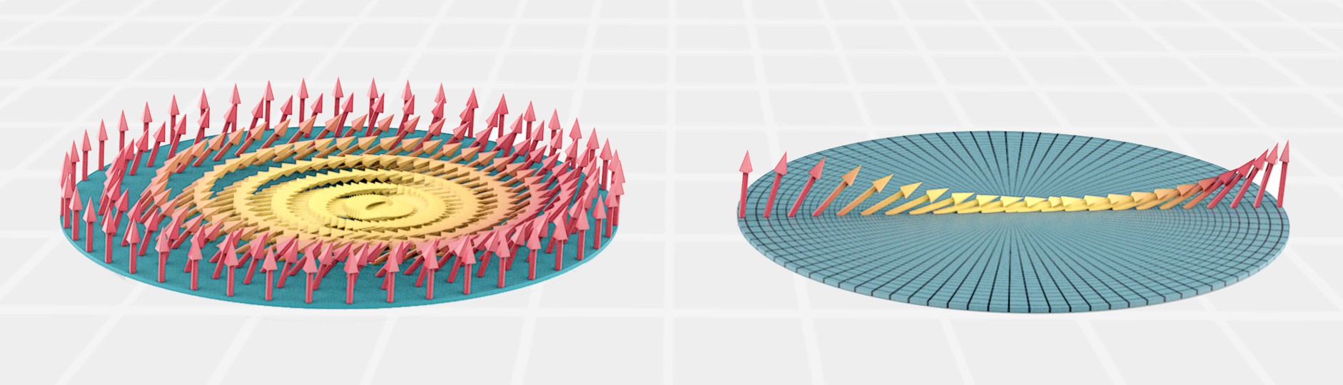
Figure 1. On the left, a minimizer of $\mathcal{E}_{\kappa,\gamma}$, with $\kappa^{2}=5$, $\gamma=0.1$, in the unit disk of $\mathbb{R}^{2}$. On the right, we isolated a ray in order to visualize the profile of the minimizer better.

We also have a comparison principle for solutions with different values of $\kappa,\gamma$:

Theorem 4.

Let $N\in\mathbb{N}^{\ast}$, $\Omega\subset\mathbb{R}^{N}$ be a smooth bounded domain, and $\kappa_{1},\kappa_{2},\gamma_{1},\gamma_{2}\in[0,+\infty)$ with $\kappa_{1}\leqslant\kappa_{2}$, $\gamma_{1}\leqslant\gamma_{2}$ and $(\kappa_{1},\gamma_{1})\neq(\kappa_{2},\gamma_{2})$. If for $i=1,2$, $\varphi_{i}$ is a solution of (8) valued into $[0,\frac{\pi}{2}]$, with $(\kappa,\gamma)=(\kappa_{i},\gamma_{i})$, then we have either $\varphi_{1}=\varphi_{2}\equiv 0$, or $\varphi_{1}=\varphi_{2}\equiv\frac{\pi}{2}$, or $\varphi_{1}<\varphi_{2}$ in $\Omega$. If in addition we assume $\gamma_{2}\char 62\relax 0$, then in the latter case we actually have $\varphi_{1}<\varphi_{2}$ on $\overline{\Omega}$.

The statements in Theorems 1, 2, 3 and 4 hold without any assumption on the geometry of the domain $\Omega$. Our last result focuses on the case where $\Omega$ is a ball, and shows that any global minimizer of $\mathcal{E}_{\kappa,\gamma}$ is radially symmetric in this case, i.e., $\boldsymbol{m}=\boldsymbol{m}(|x|)$, and by Theorem 2 has values in a quadrant of a meridian (an example of a minimizer of (8) on the two-dimensional ball is illustrated in Figure 1).

Theorem 5.

Let $\kappa,\gamma\in[0,+\infty)$. Let $\Omega=B_{R}$ be a ball of radius $R\char 62\relax 0$ centered at the origin in $\mathbb{R}^{N}$, then any global minimizer $\boldsymbol{m}$ of $\mathcal{E}_{\kappa,\gamma}$ is radially symmetric. More precisely, there exists $\sigma\in O(3,\boldsymbol{e}_{3})$ such that

$$\sigma\circ\boldsymbol{m}(x)=\Bigl{(}\sin\Bigl{(}\frac{u(\lvert x\rvert)}{2}\Bigr{)},0,\cos\Bigl{(}\frac{u(\lvert x\rvert)}{2}\Bigr{)}\Bigr{)}\quad\text{in }\Omega$$

for some non-increasing $\mathcal{C}^{\infty}$ function $u:[0,R]\to[0,\pi]$ which solves the nonlinear ODE

$$u^{\prime\prime}(r)+\frac{N-1}{r}\,u^{\prime}+\kappa^{2}\sin u=0\quad\text{in $(0,R)$},$$ (10)

$$u^{\prime}(0)=0,$$ (11)

with either a Dirichlet condition or a nonlinear Robin boundary condition at $r=R$, namely

$$\begin{cases}u(R)=0&\text{if $\gamma=0$,}\\ u^{\prime}(R)+\frac{1}{\gamma^{2}}\sin u(R)=0&\text{if $\gamma\char 62\relax 0$.}\end{cases}$$ (12)

By Theorem 3, the function $u$ in Theorem 5 is unique when $\gamma\in[0,+\infty)$. It is either the steady state $u\in\{0,\pi\}$ or a decreasing function into $(0,\pi)$.

1.3. Outline

The paper is organized as follows. In Section 2, we prove the minimality of universal configurations in a specific range of the parameters $\kappa,\gamma$ (Theorem 1). For that, we need a Poincaré-type inequality with a boundary term, which is proved in Lemma 1. Section 3 is devoted to the analysis of symmetries of the minimizers and their range, there we prove Theorem 2. In Section 4, we show the uniqueness of minimizers of $\mathcal{E}_{\kappa,\gamma}$ for $\gamma\in[0,+\infty)$ up to isometries in $O(3,\boldsymbol{e}_{3})$, see Theorem 3. In Section 5 we prove our comparison result (Theorem 4) which states that solutions of (8) are order preserving in $\kappa$ and $\gamma$. Finally, in Section 6, we focus on the case when the domain is a ball, and we prove radial symmetry and monotonicity of solutions of (8) (Theorem 5).

2. Minimality of universal configurations: Proof of Theorem 1

To investigate the minimality of the constant out-of-plane configurations $\pm\boldsymbol{e}_{3}$ we need the following Poincaré-type inequality, which can be of some interest on its own.

Lemma 1 (Poincaré-type inequality).

Let $\Omega\subseteq\mathbb{R}^{N}$ be a bounded smooth domain. Then, there exists $c_{\Omega}\char 62\relax 0$ such that for every $u\in H^{1}\left(\Omega\right)$ and every $\delta\char 62\relax 0$, we have

$$\delta\left(c_{\Omega}-\delta\right)\int_{\Omega}u^{2}(x)\mathrm{d}x\;\leqslant\int_{\Omega}\left|\nabla u(x)\right|^{2}\mathrm{d}x+\delta\int_{\partial\Omega}u^{2}(x)\mathrm{d}\mathcal{H}^{N-1}(x).$$ (13)

Moreover, in the previous relation, the constant $c_{\Omega}$ can be taken $c_{\Omega}=\frac{N}{\operatorname{diam}\left(\Omega\right)}$.

Proof.

We argue along the lines in [6]. Without loss of generality, we can assume that $0\in\Omega$. Also, by density, it is sufficient to prove (13) for every $u\in\mathcal{C}^{\infty}\left(\overline{\Omega}\right)$. By the divergence theorem we have

$$\int_{\Omega}\left(2u(x)\nabla u(x)\cdot x+Nu^{2}(x)\right)\mathrm{d}x\;=\;\int_{\Omega}\mathrm{{div}}[u^{2}(x)x]\mathrm{d}x\;=\;\int_{\partial\Omega}u^{2}(x)\boldsymbol{n}(x)\cdot x\,\mathrm{d}\mathcal{H}^{N-1}(x),$$

where, for a.e. $x\in\partial\Omega$, we denoted by $\boldsymbol{n}(x)$ the outward-point unit normal at $x\in\partial\Omega$. By Young’s inequality, it follows that for every $\delta\char 62\relax 0$ one has

$$N\int_{\Omega}u^{2}(x)\mathrm{d}x\leqslant\sup_{x\in\partial\Omega}|x|\int_{\partial\Omega}u^{2}(x)\mathrm{d}\mathcal{H}^{N-1}(x)+\sup_{x\in\Omega}|x|\int_{\Omega}\left[\frac{1}{\delta}\left|\nabla u(x)\right|^{2}+\delta u^{2}(x)\right]\mathrm{d}x.$$

Since $\sup_{x\in\partial\Omega}|x|\leqslant\mathrm{\operatorname{diam}}\left(\Omega\right)$ and $\sup_{x\in\Omega}|x|\leqslant\mathrm{\operatorname{diam}}\left(\Omega\right)$, we have

$$\left(N-\delta\mathrm{\,\operatorname{diam}}\left(\Omega\right)\right)\int_{\Omega}u^{2}(x)\mathrm{d}x\leqslant\frac{\mathrm{\mathrm{\operatorname{diam}}\left(\Omega\right)}}{\delta}\int_{\Omega}\left|\nabla u(x)\right|^{2}\mathrm{d}x+\mathrm{\mathrm{\operatorname{diam}}\left(\Omega\right)}\int_{\partial\Omega}u^{2}(x)\mathrm{d}\mathcal{H}^{N-1}(x).$$

From the previous estimate, we get that for every $\delta\char 62\relax 0$ there holds

$$\delta\left(c_{\Omega}-\delta\right)\int_{\Omega}u^{2}(x)\mathrm{d}x\;\leqslant\int_{\Omega}\left|\nabla u(x)\right|^{2}\mathrm{d}x+\delta\int_{\partial\Omega}u^{2}(x)\mathrm{d}\mathcal{H}^{N-1}(x),$$

with $c_{\Omega}\coloneqq\frac{N}{\operatorname{diam}\left(\Omega\right)}$. This concludes the proof. ∎

Proof of Theorem 1, item i.

We first consider the case where $\gamma\char 62\relax 0$. Without loss of generality, we can focus on the configuration $\boldsymbol{m}=+\boldsymbol{e}_{3}$. We observe that for any $\boldsymbol{v}\in H^{1}(\Omega,\mathbb{R}^{3})$ such that $|\boldsymbol{v}+\boldsymbol{e}_{3}|=1$ or, equivalently, such that $\left|\boldsymbol{v}\right|^{2}=-2\left(\boldsymbol{v}\cdot\boldsymbol{e}_{3}\right)$, we have

$$\mathcal{E}_{\kappa,\gamma}(\boldsymbol{e}_{3}+\boldsymbol{v})-\mathcal{E}_{\kappa,\gamma}(\boldsymbol{e}_{3}) =\int_{\Omega}\left|\nabla\boldsymbol{v}\right|^{2}+\kappa^{2}\int_{\Omega}\left(\boldsymbol{v}\cdot\boldsymbol{e}_{3}\right)^{2}+2\left(\boldsymbol{v}\cdot\boldsymbol{e}_{3}\right)+\frac{1}{\gamma^{2}}\int_{\partial\Omega}\lvert\boldsymbol{v}\times\boldsymbol{e}_{3}\rvert^{2}$$

$$=\int_{\Omega}\left|\nabla\boldsymbol{v}\right|^{2}-\kappa^{2}\int_{\Omega}|\boldsymbol{v}_{\bot}|^{2}\;+\;\frac{1}{\gamma^{2}}\int_{\partial\Omega}|\boldsymbol{v}_{\bot}|^{2},$$ (14)

with $\boldsymbol{v}_{\bot}=\boldsymbol{v}-\left(\boldsymbol{v}\cdot\boldsymbol{e}_{3}\right)\boldsymbol{e}_{3}$. Estimating the energy increment $\mathcal{E}_{\kappa,\gamma}(\boldsymbol{e}_{3}+\boldsymbol{v})-\mathcal{E}_{\kappa,\gamma}(\boldsymbol{e}_{3})$ through the Poincaré inequality (13) we get for every $\delta\char 62\relax 0$,

$$\mathcal{E}_{\kappa,\gamma}(\boldsymbol{e}_{3}+\boldsymbol{v})-\mathcal{E}_{\kappa,\gamma}(\boldsymbol{e}_{3}) \geqslant\delta\left(c_{\Omega}-\delta\right)\int_{\Omega}|\boldsymbol{v}_{\bot}|^{2}-\delta\int_{\partial\Omega}|\boldsymbol{v}_{\bot}|^{2}-\kappa^{2}\int_{\Omega}|\boldsymbol{v}_{\bot}|^{2}\;+\;\frac{1}{\gamma^{2}}\int_{\partial\Omega}|\boldsymbol{v}_{\bot}|^{2}$$

$$\geqslant\left(\delta\,\left(c_{\Omega}-\delta\right)-\kappa^{2}\right)\int_{\Omega}|\boldsymbol{v}_{\bot}|^{2}+\left(\;\frac{1}{\gamma^{2}}-\delta\right)\int_{\partial\Omega}|\boldsymbol{v}_{\bot}|^{2}.$$ (15)

If we set $\delta_{\gamma}\coloneqq\min\{\frac{c_{\Omega}}{2},\frac{1}{\gamma^{2}}\}$ and $\kappa_{\gamma}\coloneqq(\delta_{\gamma}(c_{\Omega}-\delta_{\gamma}))^{1/2}\char 62\relax 0$, then for every $\kappa\in[0,\kappa_{\gamma})$ there exists $\delta\in(0,\delta_{\gamma})$ such that $\delta\,\left(c_{\Omega}-\delta\right)\char 62\relax\kappa^{2}$ and $\frac{1}{\gamma^{2}}\char 62\relax\delta$. Hence, by (15), $\boldsymbol{e}_{3}$ (and so $-\boldsymbol{e}_{3}$) is a minimum point of $\mathcal{E}_{\kappa,\gamma}$, and any other minimum point $\boldsymbol{m}$ can only be obtained by perturbations in the $\boldsymbol{e}_{3}$ direction. This means that the constant out-of-plane vector fields $\pm\boldsymbol{e}_{3}$ are the only minimizers of $\mathcal{E}_{\kappa,\gamma}$.

A simpler argument gives a similar result for $\mathcal{E}_{\kappa,0}$. Indeed, in this case, $\boldsymbol{v}\in H^{1}_{0}(\Omega,\mathbb{R}^{3})$ and (14) reads as

$$\mathcal{E}_{\kappa,0}(\boldsymbol{e}_{3}+\boldsymbol{v})-\mathcal{E}_{\kappa,0}(\boldsymbol{e}_{3})=\int_{\Omega}\left|\nabla\boldsymbol{v}\right|^{2}-\kappa^{2}\int_{\Omega}|\boldsymbol{v}_{\bot}|^{2}.$$

But then the result follows from classical Poincaré inequality in $H^{1}_{0}(\Omega,\mathbb{R}^{3})$, by taking $\kappa_{0}\coloneqq c_{\Omega}$ where $c_{\Omega}$ is the Poincaré constant. ∎

Proof of Theorem 1, item ii.

The range of parameters under which the minimality of the constant in-plane configurations holds depends essentially on $\gamma$, and can be easily investigated through the classical trace inequality:

$$c_{\partial\Omega}\|u\|_{L^{2}\left(\partial\Omega\right)}\leqslant\|u\|_{H^{1}\left(\Omega\right)},$$ (16)

for some $c_{\partial\Omega}\char 62\relax 0$ and every $u\in H^{1}\left(\Omega\right)$. Indeed, let $\boldsymbol{e}_{\bot}\in\mathbb{S}^{2}$ such that $\boldsymbol{e}_{\bot}\cdot\boldsymbol{e}_{3}=0$ and let $\boldsymbol{v}\in H^{1}(\Omega,\mathbb{R}^{3})$ such that $|\boldsymbol{v}+\boldsymbol{e}_{\bot}|=1$. A simple computation gives that

$$\lvert(\boldsymbol{v}+\boldsymbol{e}_{\bot})\times\boldsymbol{e}_{3}\rvert^{2}-\lvert\boldsymbol{e}_{\bot}\times\boldsymbol{e}_{3}\rvert^{2} =\lvert\boldsymbol{v}\times\boldsymbol{e}_{3}\rvert^{2}+2(\boldsymbol{v}\times\boldsymbol{e}_{3})\cdot(\boldsymbol{e}_{\bot}\times\boldsymbol{e}_{3})$$

$$=\lvert\boldsymbol{v}\times\boldsymbol{e}_{3}\rvert^{2}+2\boldsymbol{v}\cdot\boldsymbol{e}_{\bot}$$

$$=\lvert\boldsymbol{v}\times\boldsymbol{e}_{3}\rvert^{2}-\lvert\boldsymbol{v}\rvert^{2}$$

$$=-(\boldsymbol{v}\cdot\boldsymbol{e}_{3})^{2}.$$

Hence, we have

$$\mathcal{E}_{\kappa,\gamma}(\boldsymbol{e}_{\bot}+\boldsymbol{v})-\mathcal{E}_{\kappa,\gamma}(\boldsymbol{e}_{\bot}) =\int_{\Omega}\left|\nabla\boldsymbol{v}\right|^{2}+\kappa^{2}\int_{\Omega}\left(\boldsymbol{v}\cdot\boldsymbol{e}_{3}\right)^{2}-\frac{1}{\gamma^{2}}\int_{\partial\Omega}(\boldsymbol{v}\cdot\boldsymbol{e}_{3})^{2}$$

$$\geqslant\int_{\Omega}\left|\nabla\boldsymbol{v}_{\bot}\right|^{2}+\left(c^{2}_{\partial\Omega}\cdot\min\{1,\kappa^{2}\}-\frac{1}{\gamma^{2}}\right)\int_{\partial\Omega}\left(\boldsymbol{v}\cdot\boldsymbol{e}_{3}\right)^{2},$$

where $\boldsymbol{v}_{\bot}=\boldsymbol{v}-\left(\boldsymbol{v}\cdot\boldsymbol{e}_{3}\right)\boldsymbol{e}_{3}$. Therefore, as soon as

$$\gamma\geqslant\gamma_{\kappa}\coloneqq\frac{1}{c_{\partial\Omega}\cdot\min\{1,\kappa\}},$$

we obtain that $\boldsymbol{e}_{\bot}$ is a global minimizer of $\mathcal{E}_{\kappa,\gamma}$. Moreover, if $\gamma\char 62\relax\gamma_{\kappa}$, we have that the constant in-plane vector fields $\boldsymbol{e}_{\bot}\in\mathbb{S}^{2}$, with $\boldsymbol{e}_{\bot}\cdot\boldsymbol{e}_{3}=0$, are the only minimizers of $\mathcal{E}_{\kappa,\gamma}$. Indeed, if $\mathcal{E}_{\kappa,\gamma}(\boldsymbol{e}_{\bot}+\boldsymbol{v})-\mathcal{E}_{\kappa,\gamma}(\boldsymbol{e}_{\bot})=0$ then $\boldsymbol{v}_{\bot}$ is constant a.e. in $\Omega$ and, therefore, so is $(\boldsymbol{v}\cdot\boldsymbol{e}_{3})$ due to constraint $|\boldsymbol{e}_{\bot}+\boldsymbol{v}|=1$ imposed on $\boldsymbol{v}$. Since $\boldsymbol{v}\cdot\boldsymbol{e}_{3}=0$ a.e. on $\partial\Omega$, we conclude that $\boldsymbol{v}$ is constant and in-plane. This concludes the proof. ∎

3. Symmetries in the target space and range of minimizers

In this section we show that due to symmetry of the problem the range of any minimizer is contained in a meridian of $\mathbb{S}^{2}$.

3.1. Symmetries of the energy functional in the target space

First, it is clear that the energy is invariant under the group of isometries that preserve the vertical coordinate axis $\mathbb{R}\boldsymbol{e}_{3}$, i.e.,

$$O(3,\boldsymbol{e}_{3})\coloneqq\left\{\sigma\in O(3)\,:\,\sigma\left(\boldsymbol{e}_{3}\right)=\boldsymbol{e}_{3}\text{ or }\sigma\left(\boldsymbol{e}_{3}\right)=-\boldsymbol{e}_{3}\right\}.$$

This group is generated by the isotropy group $\{\sigma\in O(3)\,:\,\sigma(\boldsymbol{e}_{3})=\boldsymbol{e}_{3}\}$ and the reflection $\sigma_{\boldsymbol{e}_{3}}$ through the plane orthogonal to $\boldsymbol{e}_{3}$.

Proposition 1.

For every $\kappa,\gamma\in[0,+\infty)$, $\sigma\in O(3,\boldsymbol{e}_{3})$ and $\boldsymbol{m}\in H^{1}(\Omega,\mathbb{S}^{2})$ we have $\mathcal{E}_{\kappa,\gamma}(\boldsymbol{m})=\mathcal{E}_{\kappa,\gamma}(\sigma\circ\boldsymbol{m})$.

Proposition 1 applies in particular to the reflection $\sigma=\sigma_{\boldsymbol{v}}$, defined by $\sigma_{\boldsymbol{v}}(\boldsymbol{w})=\boldsymbol{w}-2(\boldsymbol{v}\cdot\boldsymbol{w})\boldsymbol{v}$, through the plane orthogonal to a vector $\boldsymbol{v}\in\mathbb{S}^{2}$ which is either equal to $\boldsymbol{e}_{3}$ or orthogonal to $\boldsymbol{e}_{3}$. Using the fact that the $H^{1}$ seminorm is preserved by taking the positive or negative parts, we also have the following result.

Proposition 2.

Let $\kappa\in[0,+\infty)$, $\boldsymbol{v}\in\mathbb{S}^{2}$ and $\boldsymbol{m}\in H^{1}(\Omega,\mathbb{S}^{2})$. If either $\boldsymbol{v}=\boldsymbol{e}_{3}$ or $\boldsymbol{v}\cdot\boldsymbol{e}_{3}=0$, then $\mathcal{E}_{\kappa,\gamma}(\boldsymbol{m})=\mathcal{E}_{\kappa,\gamma}(\sigma_{\boldsymbol{v}}^{+}\circ\boldsymbol{m})$, where

$$\sigma_{\boldsymbol{v}}^{+}(\boldsymbol{w})\coloneqq\left\{\begin{array}[]{ll}\boldsymbol{w}&\text{if }\boldsymbol{w}\cdot\boldsymbol{v}\geqslant 0,\\ \boldsymbol{w}-2(\boldsymbol{v}\cdot\boldsymbol{w})\boldsymbol{v}&\text{if }\boldsymbol{w}\cdot\boldsymbol{v}<0.\end{array}\right.$$ (17)

This applies for instance to $\left(\sigma_{\boldsymbol{e}_{1}}^{+}\circ\boldsymbol{m}\right)=(\lvert m_{1}\rvert,m_{2},m_{3})$, $\left(\sigma_{\boldsymbol{e}_{2}}^{+}\circ\boldsymbol{m}\right)=(m_{1},\lvert m_{2}\rvert,m_{3})$ and $\left(\sigma_{\boldsymbol{e}_{3}}^{+}\circ\boldsymbol{m}\right)=(m_{1},m_{2},\lvert m_{3}\rvert)$.

3.2. Regularity of minimizers

For a smooth bounded domain $\Omega\subset\mathbb{R}^{2}$, the regularity of minimizers follows from the classical regularity theory of Schoen-Uhlenbeck [34]. However the regularity in dimension $N\geqslant 3$ is not trivially guaranteed in our problem, as there may exist singular minimizing homogeneous harmonic maps into $\mathbb{S}^{2}$ such as $x\mapsto\frac{x}{\lvert x\rvert}$ in $\mathbb{R}^{3}$. Here, we can prove regularity by using the symmetries. We start with an easy lemma.

Lemma 2.

Let $u\in W^{1,p}(\Omega)$ be a Sobolev function defined on an open set $\Omega\subset\mathbb{R}^{N}$, $p\geqslant 1$. If $\lvert u\rvert$ is continuous, then $u$ is continuous.

Proof.

If $u(x)=0$, then $u$ is continuous at $x$. If $u(x)\neq 0$, then, as $\lvert u\rvert$ is continuous, there exists a non empty ball $B_{r}(x)\subset\Omega$ where $\lvert u\rvert\geqslant\alpha\char 62\relax 0$. Let $v\in W^{1,p}(B_{r}(x))$ be defined by $v(x)\coloneqq\max\{\min\{\frac{1}{\alpha}\,u(x),1\},-1\}$. We have that $v(x)\in\{-1,1\}$ everywhere in $B_{r}(x)$, which for a Sobolev function means that $v$ is equal to a constant a.e. in $B_{r}(x)$. This means that the sign of $u$ does not change on $B_{r}(x)$, i.e. that $u=\lvert u\rvert$ a.e. in $B_{r}(x)$ or $u=-\lvert u\rvert$ a.e. in $B_{r}(x)$. Thus, $u$ is continuous. ∎

Proposition 3.

Let $\kappa,\gamma\in[0,+\infty)$ and let $\boldsymbol{m}\in H^{1}(\Omega,\mathbb{S}^{2})$ be a global minimizer of $\mathcal{E}_{\kappa,\gamma}$. Then $\boldsymbol{m}\in\mathcal{C}^{\infty}(\Omega,\mathbb{S}^{2})$.

Remark 3.1.

Below, in the proof of Theorem 2, we show that actually global minimizers of $\mathcal{E}_{\kappa,\gamma}$ are in $\mathcal{C}^{\infty}(\overline{\Omega},\mathbb{S}^{2})$, i.e., smooth up to the boundary.

Proof.

By Proposition 2, $\tilde{\boldsymbol{m}}\coloneqq(\lvert m_{1}\rvert,\lvert m_{2}\rvert,\lvert m_{3}\rvert)$ is still a global minimizer of $\mathcal{E}_{\kappa,\gamma}$. In particular, $\tilde{\boldsymbol{m}}$ is a global minimizer of $\mathcal{E}_{\kappa}$ under its own boundary condition. Since $\tilde{\boldsymbol{m}}$ is valued into a strictly convex subset of the sphere $\mathbb{S}^{2}$ and since $\mathcal{E}_{\kappa}$ is nothing but a perturbation of the Dirichlet energy by a lower order term (namely, the zero-order term of energy density $\kappa^{2}(\boldsymbol{m}\cdot\boldsymbol{e}_{3})^{2}$), we deduce from [34, Theorem IV and its corollary] that $\tilde{\boldsymbol{m}}$ is continuous in $\Omega$. Hence $\boldsymbol{m}$ is continuous by Lemma 2. But it is then standard to prove that $\boldsymbol{m}$ is smooth (we refer to [35, §2.10 and §3.2], for instance). ∎

3.3. Range of minimizers

We start with the following consequence of the maximum principle.

Lemma 3.

Let $\kappa,\gamma\in[0,+\infty)$ and $\boldsymbol{v}\in\mathbb{S}^{2}$ such that either $\boldsymbol{v}\cdot\boldsymbol{e}_{3}=0$ or $\boldsymbol{v}\in\{-\boldsymbol{e}_{3},\boldsymbol{e}_{3}\}$. If $\boldsymbol{m}$ is a global minimizer of $\mathcal{E}_{\kappa,\gamma}$, then either $\boldsymbol{m}\cdot\boldsymbol{v}\equiv 0$ in $\Omega$ or $\boldsymbol{m}\cdot\boldsymbol{v}$ never vanishes in $\Omega$.

Proof.

By Proposition 2, $\sigma_{\boldsymbol{v}}^{+}\circ\boldsymbol{m}$ is still a minimizer of $\mathcal{E}_{\kappa,\gamma}$. By Proposition 3, $\sigma_{\boldsymbol{v}}^{+}\circ\boldsymbol{m}$ is smooth. In particular, $\sigma_{\boldsymbol{v}}^{+}\circ\boldsymbol{m}$ (and not only $\boldsymbol{m}$) solves the Euler-Lagrange equation (4); projecting this equation on $\boldsymbol{v}$, we obtain that $\left(\sigma_{\boldsymbol{v}}^{+}\circ\boldsymbol{m}\right)\cdot\boldsymbol{v}=\left|\boldsymbol{m}\cdot\boldsymbol{v}\right|$ solves the elliptic equation

$$\Delta\left|\boldsymbol{m}\cdot\boldsymbol{v}\right|+c(x)\left|\boldsymbol{m}\cdot\boldsymbol{v}\right|=0\hskip 10.00002pt\text{in }\Omega,$$

with

$$c(x)=\left\{\begin{array}[]{ll}\lvert\nabla\left(\sigma_{\boldsymbol{v}}^{+}\circ\boldsymbol{m}\right)\rvert^{2}+\kappa^{2}m_{3}^{2}&\text{if }\boldsymbol{v}\cdot\boldsymbol{e}_{3}=0,\\ \lvert\nabla\left(\sigma_{\boldsymbol{v}}^{+}\circ\boldsymbol{m}\right)\rvert^{2}+\kappa^{2}(m_{3}^{2}-1)&\text{if }\boldsymbol{v}=\boldsymbol{e}_{3}.\end{array}\right.$$

We then apply the maximum principle [19, Theorem 2.10] to find that either $\boldsymbol{m}\cdot\boldsymbol{v}\equiv 0$ or $\boldsymbol{m}\cdot\boldsymbol{v}$ does not vanish in $\Omega$. ∎

Proof of Theorem 2.

By Proposition 3, $\boldsymbol{m}$ is smooth. For the rest of the proof, we proceed in four steps.

Step 1. $\boldsymbol{m}$ is valued into a meridian. For $\boldsymbol{v}\in\mathbb{S}^{2}$ such that $\boldsymbol{v}\cdot e_{3}=0$, we denote by $\mathbb{S}^{2}_{+}(\boldsymbol{v})$ the closed hemisphere directed by $\boldsymbol{v}$, i.e., the closed subset of $\mathbb{S}^{2}$ obtained intersecting $\mathbb{S}^{2}$ with the closed half-space $\{z\in\mathbb{R}^{3}\,:\,z\cdot\boldsymbol{v}\geqslant 0\}$. If $\boldsymbol{m}\equiv\pm\boldsymbol{e}_{3}$ in $\Omega$ there is nothing to prove. If not, there exists $x_{0}\in\Omega$ such that the projection $\boldsymbol{m}_{\perp}(x_{0})$ of $\boldsymbol{m}(x_{0})$ onto the plane orthogonal to $\boldsymbol{e}_{3}$ is different from zero. We set $\boldsymbol{v}_{0}\coloneqq\boldsymbol{m}_{\perp}(x_{0})/|\boldsymbol{m}_{\perp}(x_{0})|$ and we claim that the target space of $\boldsymbol{m}$ is contained in the meridian passing through $\boldsymbol{v}_{0}$. By construction, we have

$$\boldsymbol{m}(x_{0})\cdot\boldsymbol{v}\char 62\relax 0\quad\text{for every }\boldsymbol{v}\in V\coloneqq\{\boldsymbol{v}\in\mathbb{S}^{2}\,:\,\boldsymbol{v}\cdot e_{3}=0,\,\boldsymbol{v}\cdot\boldsymbol{v}_{0}\char 62\relax 0\}.$$

Therefore, by Lemma 3 and the continuity of $\boldsymbol{m}$, we get that for every $x\in\Omega$ there holds

$$\boldsymbol{m}(x)\in\textstyle\bigcap_{v\in V}\mathbb{S}^{2}_{+}(\boldsymbol{v}).$$

As the intersection on the right-hand side is the meridian passing through $\boldsymbol{v}_{0}$ we conclude.

Step 2. The image of $\boldsymbol{m}$ is contained in a quarter of vertical great circle (or half of meridian). Indeed, applying again Lemma 3 to $\boldsymbol{v}=\boldsymbol{e}_{3}$, we obtain that either

$$\boldsymbol{m}\cdot\boldsymbol{e}_{3}\geqslant 0 \Omega \boldsymbol{m}\cdot\boldsymbol{e}_{3}\leqslant 0 \Omega$$ in ,    or in .

Since $O(3,\boldsymbol{e}_{3})$ acts transitively on the quadrants of meridians, we can express $\boldsymbol{m}$ in terms of a particular solution valued into the quadrant of meridian $\{m_{2}=0\}\cap\{m_{1},m_{3}\geqslant 0\}$. Namely, there exists $\sigma\in O(3,\boldsymbol{e}_{3})$ such that $\boldsymbol{m}=\sigma\circ\boldsymbol{u}$, where $\boldsymbol{u}\in\mathcal{C}^{\infty}(\Omega,\mathbb{S}^{2})$ is of the form $\boldsymbol{u}=(u_{1},0,u_{2})$ with $u_{1},u_{2}\in\mathcal{C}^{\infty}(\Omega,\mathbb{R})$ such that $u_{1}^{2}+u_{2}^{2}=1$ and $u_{1},u_{2}\geqslant 0$ in $\Omega$. We then lift the map $\boldsymbol{u}$ to $\mathbb{R}$ by writing $\boldsymbol{u}=(\sin\varphi,0,\cos\varphi)$ with $\varphi\in\mathcal{C}^{\infty}(\Omega)$ and $0\leqslant\varphi\leqslant\frac{\pi}{2}$ in $\Omega$. We conclude by noticing that Lemma 3 also tells us that either $\varphi\equiv 0$, or $\varphi\equiv\frac{\pi}{2}$, or $0<\varphi<\frac{\pi}{2}$ in $\Omega$.

Step 3. Regularity up to the boundary. In the proof of Proposition 3 we used a symmetry argument in order to apply the regularity theory of Schoen-Uhlenbeck [34] and infer that a minimizer $\boldsymbol{m}\in\mathcal{C}^{\infty}(\Omega,\mathbb{S}^{2})$; we now claim that $\boldsymbol{m}\in\mathcal{C}^{\infty}(\overline{}\Omega,\mathbb{S}^{2})$, using the previous steps. Indeed, when $\gamma\char 62\relax 0$ it is clear that the lifting $\varphi$ of $\boldsymbol{m}$ satisfies

$$-\Delta\varphi =\frac{\kappa^{2}}{2}\sin(2\varphi)\quad\text{in $\Omega$,}$$ (18)

$$\frac{\partial\varphi}{\partial\boldsymbol{n}} =-\frac{1}{2\gamma^{2}}\sin(2\varphi)\quad\text{on $\partial\Omega$}.$$ (19)

Since $\frac{1}{\gamma^{2}}\sin(2\varphi)\in H^{1/2}(\partial\Omega)$, there exists $\tilde{\varphi}\in H^{2}(\Omega)$ such that $\partial_{\boldsymbol{n}}\tilde{\varphi}=-\frac{1}{2\gamma^{2}}\sin(2\varphi)$ (see, e.g., [30, Theorem 5.8]). For the difference $\varphi-\tilde{\varphi}$ we have $\Delta(\varphi-\tilde{\varphi})\in L^{2}(\Omega)$ and $\partial_{\boldsymbol{n}}(\varphi-\tilde{\varphi})=0$ on $\partial\Omega$. Hence, by classical elliptic regularity, we have $\varphi-\tilde{\varphi}\in H^{2}(\Omega)$. It follows that $\varphi\in H^{2}(\Omega)$ and therefore $\sin(2\varphi)\in H^{2}(\Omega)$ (see e.g. [38, Proposition 3.9]) and $-\frac{1}{\gamma^{2}}\sin(2\varphi)\in H^{3/2}(\partial\Omega)$. A bootstrap argument and Sobolev embedding theorems conclude the proof. Indeed, one can iterate the construction to infer the existence for every $k\geqslant 2$ of $\tilde{\varphi}\in H^{k}(\Omega)$ such that $\Delta(\varphi-\tilde{\varphi})\in H^{k-2}(\Omega)$ and $\partial_{\boldsymbol{n}}(\varphi-\tilde{\varphi})=0$ on $\partial\Omega$. In the case $\gamma=0$ regularity up to the boundary follows from the standard elliptic regularity.

Step 4. Range of $\operatorname{tr}_{\partial\Omega}\varphi$. We now show that when $\gamma\char 62\relax 0$, if $0<\varphi<\frac{\pi}{2}$ in $\Omega$, then $0<\varphi<\frac{\pi}{2}$ on $\partial\Omega$. Let us assume that at some point $x_{0}\in\partial\Omega$ we have $\varphi(x_{0})=0$. Then we know that $\Delta(-\varphi)\geqslant 0$ and $-\varphi(x_{0})\char 62\relax-\varphi$ in $\Omega$. Using Hopf Lemma (see [15, Lemma 3.4]), we deduce that $\partial_{\boldsymbol{n}}(-\varphi)(x_{0})\char 62\relax 0$, which contradicts the boundary condition $\partial_{\boldsymbol{n}}\varphi(x_{0})=0$. Hence $\varphi(x)\char 62\relax 0$ in $\overline{\Omega}$.

Assume now that there exists $x_{0}\in\partial\Omega$ such that $\varphi(x_{0})=\frac{\pi}{2}$. Then we define $u=\varphi-\frac{\pi}{2}\leqslant 0$ and we have $0=u(x_{0})\char 62\relax u(x)$ for $x\in\Omega$. Moreover, we have

$$\Delta u-\kappa^{2}\frac{\sin(2u)}{2u}u=0\quad\hbox{ in }\ \Omega.$$

Defining $c(x)=-\kappa^{2}\frac{\sin(2u(x))}{2u(x)}$ we know that $-\kappa^{2}\leqslant c(x)\leqslant 0$. Therefore, using [15, Lemma 3.4] in the case $c(x)\leqslant 0$ we deduce that $\partial_{\boldsymbol{n}}u(x_{0})\char 62\relax 0$, which contradicts $\partial_{\boldsymbol{n}}u(x_{0})=0$ due to boundary conditions. Hence $\varphi(x)<\frac{\pi}{2}$ in $\overline{\Omega}$. ∎

4. Uniqueness of minimizers up to a symmetry

In this section we prove Theorem 3, which is a direct consequence of the following two lemmas.

Lemma 4.

Let $\boldsymbol{m}\in H^{1}(\Omega,\mathbb{S}^{2})$ and $\boldsymbol{v}\in H^{1}_{0}\left(\Omega,\mathbb{R}^{3}\right)$ satisfy $\boldsymbol{m}+\boldsymbol{v}\in\mathbb{S}^{2}$ a.e.  in $\Omega$. If $\boldsymbol{m}$ satisfies the Euler-Lagrange equations (3) and if $m_{1}\char 62\relax 0$ a.e.  in $\Omega$, then $m_{1}$ is bounded below by positive constants on compact subsets of $\Omega$ and

$$\mathcal{E}_{\kappa}(\boldsymbol{m}+\boldsymbol{v})-\mathcal{E}_{\kappa}(\boldsymbol{m})\geqslant\int_{\Omega}m_{1}^{2}\left|\nabla\left(\frac{\boldsymbol{v}}{m_{1}}\right)\right|^{2}+\kappa^{2}\int_{\Omega}(\boldsymbol{v}\cdot\boldsymbol{e}_{3})^{2}.$$ (20)

Proof of Lemma 4.

We follow the ideas of [22, Lemma A.1], [10, Theorem 4.3] and [23, Theorem 5.1]. We have

$$\mathcal{E}_{\kappa}(\boldsymbol{m}+\boldsymbol{v})-\mathcal{E}_{\kappa}(\boldsymbol{m})=\int_{\Omega}|\nabla\boldsymbol{v}|^{2}+\kappa^{2}\int_{\Omega}(\boldsymbol{v}\cdot\boldsymbol{e}_{3})^{2}+2\int_{\Omega}\nabla\boldsymbol{m}\hskip 1.19995pt:\hskip 0.89996pt\nabla\boldsymbol{v}+2\kappa^{2}\int_{\Omega}\left(\boldsymbol{m}\cdot\boldsymbol{e}_{3}\right)(\boldsymbol{v}\cdot\boldsymbol{e}_{3}).$$

Note that since $\lvert\boldsymbol{m}\rvert=\lvert\boldsymbol{m}+\boldsymbol{v}\rvert=1$ a.e., we also have $|\boldsymbol{v}|\leqslant 2$ a.e. in $\Omega$. In particular, $\boldsymbol{v}\in H^{1}_{0}\left(\Omega,\mathbb{R}^{3}\right)\cap L^{\infty}(\Omega,\mathbb{R}^{3})$. Since $\boldsymbol{m}$ satisfies the Euler-Lagrange equations (3), we get

$$\mathcal{E}_{\kappa}(\boldsymbol{m}+\boldsymbol{v})-\mathcal{E}_{\kappa}(\boldsymbol{m})=\int_{\Omega}|\nabla\boldsymbol{v}|^{2}+\kappa^{2}\int_{\Omega}(\boldsymbol{v}\cdot\boldsymbol{e}_{3})^{2}+2\int_{\Omega}(|\nabla\boldsymbol{m}|^{2}+\kappa^{2}\left(\boldsymbol{m}\cdot\boldsymbol{e}_{3}\right)^{2})\boldsymbol{m}\cdot\boldsymbol{v}.$$

On the other hand, since $\lvert\boldsymbol{m}+\boldsymbol{v}\rvert=1$, we have $2\boldsymbol{m}\cdot\boldsymbol{v}=-|\boldsymbol{v}|^{2}$ and, therefore,

$$\mathcal{E}_{\kappa}(\boldsymbol{m}+\boldsymbol{v})-\mathcal{E}_{\kappa}(\boldsymbol{m})=\int_{\Omega}|\nabla\boldsymbol{v}|^{2}+\kappa^{2}\int_{\Omega}(\boldsymbol{v}\cdot\boldsymbol{e}_{3})^{2}-\int_{\Omega}(|\nabla\boldsymbol{m}|^{2}+\kappa^{2}\left(\boldsymbol{m}\cdot\boldsymbol{e}_{3}\right)^{2})|\boldsymbol{v}|^{2}.$$ (21)

Hence, (20) will follow once we prove that for all $\boldsymbol{v}\in H^{1}_{0}\cap L^{\infty}\left(\Omega,\mathbb{R}^{3}\right)$,

$$\int_{\Omega}|\nabla\boldsymbol{v}|^{2}\geqslant\int_{\Omega}(|\nabla\boldsymbol{m}|^{2}+\kappa^{2}\left(\boldsymbol{m}\cdot\boldsymbol{e}_{3}\right)^{2})|\boldsymbol{v}|^{2}+\int_{\Omega}m_{1}^{2}\left|\nabla\left(\frac{\boldsymbol{v}}{m_{1}}\right)\right|^{2}.$$ (22)

We first assume that $\boldsymbol{v}\in C_{c}^{\infty}(\Omega,\mathbb{R}^{3})$, the general case will follow by density.

Now, by the Euler-Lagrange equation of $m_{1}$ in (3) and since $m_{1}$ is assumed to be positive in $\Omega$, we have in particular that $m_{1}$ is a positive weak superharmonic function, i.e. $\Delta m_{1}\leqslant 0$ weakly in $\Omega$; we deduce from the weak Harnack-Moser inequality (see [24, Theorem 14.1.2.]) that $m_{1}$ is bounded from below by a positive constant on the support of $\boldsymbol{v}$. Hence, we can write $\boldsymbol{v}$ in the form

$$\boldsymbol{v}=m_{1}\boldsymbol{u},$$ (23)

where $\boldsymbol{u}=\frac{\boldsymbol{v}}{m_{1}}\in H_{0}^{1}\left(\Omega,\mathbb{R}^{3}\right)\cap L^{\infty}(\Omega,\mathbb{R}^{3})$. We then compute

$$\int_{\Omega}|\nabla\boldsymbol{v}|^{2} =\sum_{j=1}^{N}\int_{\Omega}|\boldsymbol{u}\partial_{j}m_{1}+m_{1}\partial_{j}\boldsymbol{u}|^{2}$$ (24)

$$=\int_{\Omega}|\boldsymbol{u}|^{2}\left|\nabla m_{1}\right|^{2}+m_{1}^{2}\left|\nabla\boldsymbol{u}\right|^{2}+m_{1}\nabla m_{1}\cdot\nabla|\boldsymbol{u}|^{2}$$ (25)

$$=\int_{\Omega}m_{1}^{2}\left|\nabla\boldsymbol{u}\right|^{2}+\nabla m_{1}\cdot\nabla(m_{1}|\boldsymbol{u}|^{2}).$$ (26)

Now, testing the Euler-Lagrange equations (3) against $\boldsymbol{\varphi}\coloneqq m_{1}|\boldsymbol{u}|^{2}\boldsymbol{e}_{1}\in H^{1}_{0}\left(\Omega,\mathbb{R}^{3}\right)\cap L^{\infty}(\Omega,\mathbb{R}^{3})$, we obtain

$$\int_{\Omega}\nabla m_{1}\cdot\nabla(m_{1}|\boldsymbol{u}|^{2})=\int_{\Omega}(|\nabla\boldsymbol{m}|^{2}+\kappa^{2}\left(\boldsymbol{m}\cdot\boldsymbol{e}_{3}\right)^{2})m_{1}^{2}|\boldsymbol{u}|^{2}.$$ (27)

Combining the previous two relations, and recalling that $\boldsymbol{v}=m_{1}\boldsymbol{u}$, we obtain the following identity:

$$\int_{\Omega}|\nabla\boldsymbol{v}|^{2}=\int_{\Omega}m_{1}^{2}\left|\nabla\boldsymbol{u}\right|^{2}+(|\nabla\boldsymbol{m}|^{2}+\kappa^{2}\left(\boldsymbol{m}\cdot\boldsymbol{e}_{3}\right)^{2})|\boldsymbol{v}|^{2}.$$ (28)

This proves (22) in the case where $\boldsymbol{v}\in C_{c}^{\infty}(\Omega,\mathbb{R}^{3})$. In general, we have $\boldsymbol{v}\in H^{1}_{0}\left(\Omega,\mathbb{R}^{3}\right)\cap L^{\infty}(\Omega,\mathbb{R}^{3})$ and there thus exists a sequence $\left(\boldsymbol{v}_{n}\right)_{n\in\mathbb{N}}$ in $C_{c}^{\infty}(\Omega,\mathbb{R}^{3})$ such that

$$\sup_{n\in\mathbb{N}}\|\boldsymbol{v}_{n}\|_{\infty}\leqslant\|\boldsymbol{v}\|_{\infty}+1$$

and

$$\boldsymbol{v}_{n}\rightarrow\boldsymbol{v}\quad\text{in }H_{0}^{1}\left(\Omega,\mathbb{R}^{3}\right).$$ (29)

By the previous computations in the smooth case, we have for every compact $K\subset\Omega$ and $n\in\mathbb{N}$,

$$\int_{\Omega}|\nabla\boldsymbol{v}_{n}|^{2}\geqslant\int_{K}(|\nabla\boldsymbol{m}|^{2}+\kappa^{2}\left(\boldsymbol{m}\cdot\boldsymbol{e}_{3}\right)^{2})|\boldsymbol{v}_{n}|^{2}+\int_{K}m_{1}^{2}\left|\nabla\left(\frac{\boldsymbol{v}_{n}}{m_{1}}\right)\right|^{2}.$$

The conclusion follows by passing to the limit $n\rightarrow\infty$ using the dominated convergence theorem, and then taking the supremum over compacts $K\subset\Omega$ using the monotone convergence theorem. ∎

Lemma 5.

Let $\boldsymbol{m}\in H^{1}(\Omega,\mathbb{S}^{2})$ and $\boldsymbol{v}\in H^{1}\left(\Omega,\mathbb{R}^{3}\right)$ satisfy $\boldsymbol{m}+\boldsymbol{v}\in\mathbb{S}^{2}$ a.e.  in $\Omega$. If $\boldsymbol{m}$ satisfies the Euler-Lagrange equations (3) and if $m_{1},m_{3}\char 62\relax 0$ in $\overline{}\Omega$, then

$$\mathcal{E}_{\kappa,\gamma}(\boldsymbol{m}+\boldsymbol{v})-\mathcal{E}_{\kappa,\gamma}(\boldsymbol{m})\geqslant\int_{\Omega}m_{1}^{2}\lvert\nabla\boldsymbol{u}^{\perp}\rvert^{2}+m_{3}^{2}\lvert\nabla u_{3}\rvert^{2},$$ (30)

where we wrote $\boldsymbol{v}=m_{1}\boldsymbol{u}^{\perp}+m_{3}u_{3}\boldsymbol{e}_{3}$ with $\boldsymbol{u}=(\boldsymbol{u}^{\perp},u_{3})\in H^{1}(\Omega,\mathbb{R}^{3})$.

Proof of Lemma 5.

As in Lemma 4 we have

$$\mathcal{E}_{\kappa,\gamma}(\boldsymbol{m}+\boldsymbol{v})-\mathcal{E}_{\kappa,\gamma}(\boldsymbol{m}) =\int_{\Omega}|\nabla\boldsymbol{v}|^{2}+\kappa^{2}\int_{\Omega}(\boldsymbol{v}\cdot\boldsymbol{e}_{3})^{2}+2\int_{\Omega}\nabla\boldsymbol{m}\hskip 1.19995pt:\hskip 0.89996pt\nabla\boldsymbol{v}+2\kappa^{2}\int_{\Omega}\left(\boldsymbol{m}\cdot\boldsymbol{e}_{3}\right)(\boldsymbol{v}\cdot\boldsymbol{e}_{3})$$

$$\qquad-\frac{1}{\gamma^{2}}\int_{\partial\Omega}(\boldsymbol{v}\cdot\boldsymbol{e}_{3})^{2}+2(\boldsymbol{m}\cdot\boldsymbol{e}_{3})(\boldsymbol{v}\cdot\boldsymbol{e}_{3})$$ (31)

and $\boldsymbol{v}\in H^{1}\left(\Omega,\mathbb{R}^{3}\right)\cap L^{\infty}(\Omega,\mathbb{R}^{3})$. Since $\boldsymbol{m}$ satisfies the Euler-Lagrange equations (3) and $2\boldsymbol{m}\cdot\boldsymbol{v}=-|\boldsymbol{v}|^{2}$ we obtain

$$\mathcal{E}_{\kappa,\gamma}(\boldsymbol{m}+\boldsymbol{v})-\mathcal{E}_{\kappa,\gamma}(\boldsymbol{m}) =\int_{\Omega}|\nabla\boldsymbol{v}|^{2}+\kappa^{2}\int_{\Omega}(\boldsymbol{v}\cdot\boldsymbol{e}_{3})^{2}-\int_{\Omega}(|\nabla\boldsymbol{m}|^{2}+\kappa^{2}\left(\boldsymbol{m}\cdot\boldsymbol{e}_{3}\right)^{2})|\boldsymbol{v}|^{2}$$

$$\qquad-\frac{1}{\gamma^{2}}\int_{\partial\Omega}(\boldsymbol{v}\cdot\boldsymbol{e}_{3})^{2}-\left(\boldsymbol{m}\cdot\boldsymbol{e}_{3}\right)^{2}|\boldsymbol{v}|^{2}.$$ (32)

Now we use the fact $m_{1}\char 62\relax 0$, $m_{3}\char 62\relax 0$ in $\overline{\Omega}$ and represent $\boldsymbol{v}=m_{1}\boldsymbol{u}^{\perp}+m_{3}u_{3}\boldsymbol{e}_{3}$ with $\boldsymbol{u}=(\boldsymbol{u}^{\perp},u_{3})\in H^{1}(\Omega,\mathbb{R}^{3})$. In that case, we have (in the following computations, we assume that $\boldsymbol{m}$ is smooth; the general case follows similarly, as in the proof of Lemma 4)

$$\int_{\Omega}|\nabla\boldsymbol{v}|^{2} =\int_{\Omega}m_{1}^{2}\lvert\nabla\boldsymbol{u}^{\perp}\rvert^{2}+\nabla m_{1}\cdot\nabla(m_{1}|\boldsymbol{u}^{\perp}|^{2})+m_{3}^{2}\lvert\nabla u_{3}\rvert^{2}+\nabla m_{3}\cdot\nabla(m_{3}u_{3}^{2})$$ (33)

$$=\int_{\Omega}m_{1}^{2}\lvert\nabla\boldsymbol{u}^{\perp}\rvert^{2}-\Delta m_{1}\ m_{1}\lvert\boldsymbol{u}^{\perp}\rvert^{2}+\int_{\partial\Omega}\partial_{\boldsymbol{n}}m_{1}\ m_{1}\lvert\boldsymbol{u}^{\perp}\rvert^{2}$$

$$\qquad+\int_{\Omega}m_{3}^{2}\lvert\nabla u_{3}\rvert^{2}-\Delta m_{3}\ m_{3}\,u_{3}^{2}+\int_{\partial\Omega}\partial_{\boldsymbol{n}}m_{3}\ m_{3}\,u_{3}^{2}$$ (34)

$$=\int_{\Omega}m_{1}^{2}\lvert\nabla\boldsymbol{u}^{\perp}\rvert^{2}+m_{3}^{2}\lvert\nabla u_{3}\rvert^{2}+(|\nabla\boldsymbol{m}|^{2}+\kappa^{2}\left(\boldsymbol{m}\cdot\boldsymbol{e}_{3}\right)^{2})|\boldsymbol{v}|^{2}-\kappa^{2}(\boldsymbol{v}\cdot\boldsymbol{e}_{3})^{2}$$

$$\qquad+\frac{1}{\gamma^{2}}\int_{\partial\Omega}(\boldsymbol{v}\cdot\boldsymbol{e}_{3})^{2}-m_{3}^{2}|\boldsymbol{v}|^{2}.$$ (35)

Plugging it into the energy difference we obtain

$$\mathcal{E}_{\kappa,\gamma}(\boldsymbol{m}+\boldsymbol{v})-\mathcal{E}_{\kappa,\gamma}(\boldsymbol{m})=\int_{\Omega}m_{1}^{2}\lvert\nabla\boldsymbol{u}^{\perp}\rvert^{2}+m_{3}^{2}\lvert\nabla u_{3}\rvert^{2}.$$ (36)

This concludes the proof. ∎

Proof of Theorem 3.

We first consider the case $\gamma=0$. If the constant out-of-plane configurations $\pm\boldsymbol{e}_{3}$ are the only global minimizers of $\mathcal{E}_{\kappa,0}$, we are done. If not, this means by Theorem 2 that $\mathcal{E}_{\kappa,0}$ has a global minimizer of the form $\boldsymbol{m}=(\sin\varphi,0,\cos\varphi)$ with $\varphi\in H^{1}(\Omega)$ such that $0<\varphi\leqslant\frac{\pi}{2}$ a.e.  in $\Omega$. If $\bar{}\boldsymbol{m}=\boldsymbol{m}+\boldsymbol{v}$ is another minimizer with $\boldsymbol{v}\in H^{1}_{0}(\Omega,\mathbb{R}^{3})$, then we have by Lemma 4 that $\boldsymbol{v}=m_{1}\boldsymbol{v}_{0}$ for some $\boldsymbol{v}_{0}\in\mathbb{R}^{3}$. But, in order to satisfy the constraint $\boldsymbol{m}+m_{1}\boldsymbol{v}_{0}\in\mathbb{S}^{2}$, we must have $\boldsymbol{v}_{0}\cdot(m_{1}\boldsymbol{v}_{0}+2\boldsymbol{m})=0$. Restricted to the boundary $\partial\Omega$, where we have $\boldsymbol{m}=\boldsymbol{e}_{3}$, this condition yields $\boldsymbol{v}_{0}\cdot\boldsymbol{e}_{3}=0$. Hence, since $m_{2}\equiv 0$, we arrive at the equation $0=\boldsymbol{v}_{0}\cdot(m_{1}\boldsymbol{v}_{0}+2m_{1}e_{1})$ which means that $\lvert\boldsymbol{v}_{0}+e_{1}\rvert^{2}=1$. Hence, $\boldsymbol{v}_{0}=(\cos\theta-1,\sin\theta,0)$ for some $\theta\in\mathbb{R}$, which means that $\bar{}\boldsymbol{m}=(\cos\theta\sin\varphi,\sin\theta\sin\varphi,\cos\varphi)$, i.e. $\boldsymbol{m}$ is a rotation of $\boldsymbol{m}$ of angle $\theta$ around the $x_{3}$-axis.

In the case $\gamma\char 62\relax 0$ if constant in-plane or constant out-of-plane $\pm\boldsymbol{e}_{3}$ configurations are the only minimizers then the result follows by noting that $\pm\boldsymbol{e}_{3}$ and constant in-plane configurations cannot be minimizers simultaneously. Indeed, assuming that their energies coincide and are optimal, then we would have that the constant vectors $\boldsymbol{m}=(a_{1},0,a_{3})$, with $a_{1},a_{3}\char 62\relax 0$ such that $a_{1}^{2}+a_{3}^{2}=1$, have the same energy; but these configurations do not solve the Euler-Lagrange equations, contradicting the minimality.

If constant configurations are not the only minimizers, then by Theorem 2 the energy $\mathcal{E}_{\kappa,\gamma}$ has a global minimizer of the form $\boldsymbol{m}=(\sin\varphi,0,\cos\varphi)$ with $\varphi\in H^{1}(\Omega)$ such that $0<\varphi<\frac{\pi}{2}$   in $\overline{}\Omega$. If $\bar{}\boldsymbol{m}=\boldsymbol{m}+\boldsymbol{v}$ is another minimizer with $\boldsymbol{v}\in H^{1}(\Omega,\mathbb{R}^{3})$, then we have by Lemma 5 that $\boldsymbol{v}=m_{1}\boldsymbol{w}^{\perp}+m_{3}w_{3}\mathbf{\boldsymbol{e}}_{3}$ for some $\boldsymbol{w}=(\boldsymbol{w}^{\perp},w_{3})\in\mathbb{R}^{3}$. But, in order to satisfy the constraint $\boldsymbol{m}+\boldsymbol{v}\in\mathbb{S}^{2}$, we must have $w_{3}\in\{0,-2\}$ and $|\boldsymbol{w}^{\perp}+\boldsymbol{e}_{1}|=1$, implying the result. ∎

Remark 4.1.

We note that using Lemma 4 we actually proved the uniqueness (up to a symmetry) of a solution of the Euler-Lagrange equation (4) with $m_{1}\char 62\relax 0$ under boundary condition $\boldsymbol{m}=\pm\boldsymbol{e}_{3}$ for any $\kappa\char 62\relax 0$. In a similar way it is possible to prove the same result under a prescribed Dirichlet boundary conditions $\boldsymbol{g}\in H^{1/2}\left(\partial\Omega,\mathbb{S}^{2}\right)$ with either $g_{1}\char 62\relax 0$ or $g_{2}\char 62\relax 0$.

Analogously, using Lemma 5 we have proved the uniqueness (up to a symmetry) of a solution of the Euler-Lagrange equation (3) with $m_{1}\char 62\relax 0$ and $m_{3}\char 62\relax 0$ on $\overline{}\Omega$ for any $\gamma\char 62\relax 0$ and $\kappa\char 62\relax 0$.

5. Comparison of solutions

5.1. Minimizers with different penalizations

Before proving Theorem 4, we introduce the localized energy functional defined for $\kappa\geqslant 0$, $\gamma\char 62\relax 0$, $\varphi\in H^{1}(\Omega,\mathbb{R})$ and every Borel set $O\subset\mathbb{R}^{N}$, by

$$\mathcal{F}_{\kappa,\gamma}(\varphi,O)\coloneqq\int_{O\cap\Omega}\lvert\nabla\varphi\rvert^{2}+\kappa^{2}\int_{O\cap\Omega}\cos^{2}\varphi+\frac{1}{\gamma^{2}}\int_{O\cap\partial\Omega}\sin^{2}\varphi.$$ (37)

When $\gamma=0$, we also define for every Borel subset $O\subset\Omega$,

$$\mathcal{F}_{\kappa,0}(\varphi,O)\coloneqq\int_{O}\lvert\nabla\varphi\rvert^{2}+\kappa^{2}\int_{O}\cos^{2}\varphi.$$ (38)

Proof of Theorem 4.

We proceed in 5 steps.

Step 1. Energy estimates. Let $\varphi_{i}$ be a minimizer of the energy $\mathcal{E}_{\kappa_{i},\gamma_{i}}$ valued into $[0,\frac{\pi}{2}]$, with $i=1,2$. By Theorem 2 we know that $\varphi_{1}$ and $\varphi_{2}$ are smooth on $\overline{\Omega}$. We define

$$O\coloneqq\{x\in\overline{\Omega}\,:\,\varphi_{1}(x)\char 62\relax\varphi_{2}(x)\};$$

we shall see that $O=\emptyset$, i.e., $\varphi_{1}\leqslant\varphi_{2}$ on $\overline{\Omega}$. First, observe that, using $\nabla\varphi_{1}=\nabla\varphi_{2}$ a.e. on $\{\varphi_{1}=\varphi_{2}\}\cap\Omega$ and comparing the functions $\varphi_{1},\varphi_{2}$ with their minimum $\varphi_{1}\wedge\varphi_{2}$ and their maximum $\varphi\vee\varphi_{2}$, by minimality,

$$\mathcal{F}_{\kappa_{1},\gamma_{1}}(\varphi_{1},\bar{\Omega})\leqslant\mathcal{F}_{\kappa_{1},\gamma_{1}}(\varphi_{1}\wedge\varphi_{2},\bar{\Omega})\quad\text{and}\quad\mathcal{F}_{\kappa_{2},\gamma_{2}}(\varphi_{2},\bar{\Omega})\leqslant\mathcal{F}_{\kappa_{2},\gamma_{2}}(\varphi_{1}\vee\varphi_{2},\bar{\Omega}).$$ (39)

Hence, using (39), we obtain the following estimates (where if $\gamma_{1}=0$, so that $\varphi_{1}\in H^{1}_{0}(\Omega)$ and $O\subset\Omega$, all the boundary terms are ignored),

$$\mathcal{F}_{\kappa_{1},\gamma_{1}}(\varphi_{1},O) \leqslant\mathcal{F}_{\kappa_{1},\gamma_{1}}(\varphi_{2},O)$$

$$=\mathcal{F}_{\kappa_{2},\gamma_{2}}(\varphi_{2},O)+\left(\kappa_{1}^{2}-\kappa_{2}^{2}\right)\int_{O\cap\Omega}\cos^{2}\varphi_{2}+\left(\frac{1}{\gamma_{1}^{2}}-\frac{1}{\gamma_{2}^{2}}\right)\int_{O\cap\partial\Omega}\sin^{2}\varphi_{2}$$

$$\leqslant\mathcal{F}_{\kappa_{2},\gamma_{2}}(\varphi_{1},O)+(\kappa_{1}^{2}-\kappa_{2}^{2})\int_{O\cap\Omega}\cos^{2}\varphi_{2}+\left(\frac{1}{\gamma_{1}^{2}}-\frac{1}{\gamma_{2}^{2}}\right)\int_{O\cap\partial\Omega}\sin^{2}\varphi_{2}$$

$$=\mathcal{F}_{\kappa_{1},\gamma_{1}}(\varphi_{1},O)+(\kappa_{1}^{2}-\kappa_{2}^{2})\int_{O\cap\Omega}\left(\cos^{2}\varphi_{2}-\cos^{2}\varphi_{1}\right)$$

$$\qquad+\left(\frac{1}{\gamma_{1}^{2}}-\frac{1}{\gamma_{2}^{2}}\right)\int_{O\cap\partial\Omega}\left(\sin^{2}\varphi_{2}-\sin^{2}\varphi_{1}\right),$$

from which we infer that

$$(\kappa_{1}^{2}-\kappa_{2}^{2})\int_{O\cap\Omega}\bigl{(}\cos^{2}\varphi_{2}-\cos^{2}\varphi_{1}\bigr{)}+\left(\frac{1}{\gamma_{1}^{2}}-\frac{1}{\gamma_{2}^{2}}\right)\int_{O\cap\partial\Omega}\bigl{(}\sin^{2}\varphi_{2}-\sin^{2}\varphi_{1}\bigr{)}\geqslant 0.$$

Now we use the assumption $\kappa_{1}\leqslant\kappa_{2}$, $\gamma_{1}\leqslant\gamma_{2}$ and $(\kappa_{1},\gamma_{1})\neq(\kappa_{2},\gamma_{2})$. Noticing that $x\mapsto\cos^{2}(x)$ is decreasing and $x\mapsto\sin^{2}(x)$ is increasing on $[0,\frac{\pi}{2}]$, and that $\varphi_{2}<\varphi_{1}$ on $O$ by definition, it entails

$$\begin{cases}O\cap\Omega=\emptyset&\text{if $\kappa_{1}<\kappa_{2}$,}\\ O\cap\partial\Omega=\emptyset&\text{if $\gamma_{1}<\gamma_{2}$}.\end{cases}$$ (40)

(Note that when $\gamma_{1}=0$, the second assertion is not a consequence of the previous estimates, but it is trivially satisfied because $\varphi_{1}=0$ on $\partial\Omega$ and $O\subset\Omega$ in this case.)

The first assertion means that

$$\varphi_{1}\leqslant\varphi_{2}\quad\text{in $\overline{\Omega}$ if $\kappa_{1}<\kappa_{2}$.}$$ (41)

When $\kappa_{1}=\kappa_{2}$, we need more work:

Step 2. Comparison of solutions when $\kappa_{1}=\kappa_{2}=:\kappa$ and $\gamma_{1}<\gamma_{2}$. By (40), we have

$$\varphi_{1}\leqslant\varphi_{2}\quad\text{on }\partial\Omega.$$ (42)

Hence, $\varphi_{1}=\varphi_{1}\wedge\varphi_{2}$ and $\varphi_{2}=\varphi_{1}\vee\varphi_{2}$ on $\partial\Omega$. By minimality (cf. Remark 4.1) this yields

$$\mathcal{E}_{\kappa}(\varphi_{1})\leqslant\mathcal{E}_{\kappa}(\varphi_{1}\wedge\varphi_{2})\quad\text{and}\quad\mathcal{E}_{\kappa}(\varphi_{2})\leqslant\mathcal{E}_{\kappa}(\varphi_{1}\vee\varphi_{2}).$$

Since we have also $\mathcal{E}_{\kappa}(\varphi_{1})+\mathcal{E}_{\kappa}(\varphi_{2})=\mathcal{E}_{\kappa}(\varphi_{1}\wedge\varphi_{2})+\mathcal{E}_{\kappa}(\varphi_{1}\vee\varphi_{2})$, we obtain that

$$\mathcal{E}_{\kappa}(\varphi_{1})=\mathcal{E}_{\kappa}(\varphi_{1}\wedge\varphi_{2})\quad\text{and}\quad\mathcal{E}_{\kappa}(\varphi_{2})=\mathcal{E}_{\kappa}(\varphi_{1}\vee\varphi_{2}).$$

The first equality means that both $\varphi_{1}$ and $\varphi_{1}\wedge\varphi_{2}$ minimize $\mathcal{E}_{\kappa}$ under their own Dirichlet boundary condition on $\partial\Omega$; in particular, they solve the Euler-Lagrange equation $-\Delta u=\kappa^{2}\sin u$ in the variable $u=2\varphi$. By uniqueness for positive solutions to sublinear elliptic equations with Dirichlet boundary conditions (see [1, Appendix II]), we deduce that either $\varphi_{1}\equiv 0$, or $\varphi_{1}\wedge\varphi_{2}\equiv 0$, or $\varphi_{1}\equiv\varphi_{1}\wedge\varphi_{2}$. In the case where $\varphi_{1}\wedge\varphi_{2}\equiv 0$ but $\varphi_{1}$ is not identically $0$, since $\Delta\varphi_{2}\leqslant 0$, we deduce from the strong maximum principal that $\varphi_{2}\equiv 0$; in particular, $\varphi_{1}=0$ on $\partial\Omega$ by (42), and we deduce from our uniqueness result for minimizers under homogeneous Dirichlet boundary conditions Theorem 3, that $\varphi_{1}\equiv\varphi_{2}(\equiv 0)$ on $\Omega$. In any case, we have proved that

$$\varphi_{1}\leqslant\varphi_{2}\quad\text{on $\overline{}\Omega$ if $\gamma_{1}<\gamma_{2}$}.$$ (43)

Step 4. Strict comparison of solutions in $\Omega$. We know that $u_{i}=2\varphi_{i}$ solve the Euler–Lagrange equations associated with $\mathcal{E}_{\kappa_{i},\gamma_{i}}$,

$$-\Delta u_{i} =\kappa_{i}^{2}\sin(u_{i})\quad\text{in $\Omega$,}$$ (44)

$$\frac{\partial u_{i}}{\partial\boldsymbol{n}} =-\frac{1}{\gamma_{i}^{2}}\sin u_{i}\quad\text{on $\partial\Omega$ if $0<\gamma_{i}$ (and $u_{i}\equiv 0$ on $\partial\Omega$ if $\gamma_{i}=0$)},$$ (45)

and that, by (41) and (43),

$$u_{1}\leqslant u_{2}\quad\text{in $\overline{\Omega}$.}$$ (46)

Using that $u\mapsto u+\sin u$ is non decreasing and that $\kappa_{1}\leqslant\kappa_{2}$, we find that

$$-\Delta(u_{2}-u_{1})+\kappa_{1}^{2}(u_{2}-u_{1})\geqslant\kappa_{1}^{2}(\sin(u_{2})+u_{2}-\sin(u_{1})-u_{1})\geqslant 0\quad\text{in $\Omega$}.$$ (47)

By the strong maximum principal, we obtain that either $u_{2}\equiv u_{1}$ in $\Omega$, or $u_{1}<u_{2}$ in $\Omega$.

In the first case, i.e., $u_{1}\equiv u_{2}$, we deduce by (44) that if $\kappa_{1}<\kappa_{2}$ then either $u_{1}=u_{2}\equiv 0$ or $u_{1}=u_{2}\equiv\pi$ in $\Omega$; when $\kappa_{1}=\kappa_{2}$ and $\gamma_{1}<\gamma_{2}$, we have by (45) that either $u_{1}=u_{2}\equiv\pi$ or $u_{1}=u_{2}\equiv 0$ on $\partial\Omega$ and by Hopf lemma it follows that $u_{1}$ and $u_{2}$ are constants in $\Omega$ since $\frac{\partial u_{i}}{\partial\boldsymbol{n}}\equiv 0$ on $\partial\Omega$.

Step 5. Strict comparison of solutions on $\partial\Omega$ when $u_{1}<u_{2}$ in $\Omega$ and $\gamma_{2}\char 62\relax 0$. In this case, we want to show that $u_{1}<u_{2}$ on $\partial\Omega$. Assume there is $x_{0}\in\partial\Omega$ such that $u_{1}(x_{0})=u_{2}(x_{0})$ then by Hopf lemma we obtain $\frac{\partial(u_{2}-u_{1})}{\partial\boldsymbol{n}}(x_{0})<0$. If $0<\gamma_{1}\leqslant\gamma_{2}$ then using (45) we deduce that $\frac{\partial(u_{2}-u_{1})(x_{0})}{\partial\boldsymbol{n}}\geqslant 0$, obtaining the contradiction. If $\gamma_{1}=0<\gamma_{2}$, we know that $u_{1}=0$ on $\partial\Omega$; hence $u_{2}(x_{0})=0$ and, by (45), $\frac{\partial u_{2}}{\partial\boldsymbol{n}}(x_{0})=0$. Applying Hopf lemma to $u_{2}$ we obtain that $u_{2}\equiv 0$ in $\overline{\Omega}$, thus contradicting the fact that $u_{1}<u_{2}$ in $\Omega$. Therefore if $\gamma_{2}\char 62\relax 0$ we have $u_{2}\char 62\relax u_{1}$ on $\overline{}\Omega$. ∎

6. Radial symmetry of minimizers in a ball: Proof of Theorem 5

Numerical simulations suggest that when the domain $\Omega$ has spherical symmetry, the minimizers of $\mathcal{E}_{\kappa,\gamma}$ are radially symmetric (cf. Figure 1). The aim of this section is to turn this observation into a quantitative statement.

The proof we give below for the radial symmetry of minimizers $\mathcal{E}_{\kappa,\gamma}$ also works for the boundary value problem associated with $\mathcal{E}_{\kappa,0}$. However, radiality of the minimizers of $\mathcal{E}_{\kappa,0}$ immediately follows from a celebrated result of Gidas-Ni-Nirenberg [14] about radial symmetry for semilinear elliptic equations. We give the details below.

Proposition 4.

If $\Omega$ is a ball centered at the origin, then any minimizer $\boldsymbol{m}$ of the energy $\mathcal{E}_{\kappa,0}$ is radially symmetric. More precisely, $\boldsymbol{m}$ is either constant with $\boldsymbol{m}\cdot\boldsymbol{e}_{3}\in\{0,-1,1\}$, or there exist $\sigma\in O(3,\boldsymbol{e}_{3})$ and a solution ${\varphi}:\mathbb{R}^{+}\to(0,\frac{\pi}{2})$ in (9) such that

$$\boldsymbol{m}(x)=\sigma\circ(\sin{\varphi}(\lvert x\rvert),0,\cos{\varphi}(\lvert x\rvert))\quad\text{a.e.\ in }\Omega.$$

Proof of Proposition 4.

Without loss of generality, one can assume that $\boldsymbol{m}$ is not constant. By Theorem 2, there exists $\sigma\in O(3,\boldsymbol{e}_{3})$ and a solution $\varphi\in H_{0}^{1}(\Omega)\cap\mathcal{C}^{\infty}(\overline{}\Omega)$ of (9) such that $\boldsymbol{m}=\sigma(\sin\varphi,0,\cos\varphi)$ and $0<\varphi<\frac{\pi}{2}$ in $\Omega$. In particular, $\varphi$ solves the Euler-Lagrange equation $\Delta(2\varphi)+\kappa^{2}\sin(2\varphi)=0$ in $\Omega$. The radial symmetry of $\varphi$ then follows from [14]. ∎

In the case of the penalization of the boundary datum, we use a reflection method introduced in [26] and the unique continuation principle for elliptic equations (see, for instance, [29]). Note that this method also works for the boundary value problem associated with $\mathcal{E}_{\kappa,0}$, and the following proof also covers Proposition 4.

Proof of Theorem 5.

We concentrate on the case $\gamma\char 62\relax 0$. Without loss of generality, one can assume that $\boldsymbol{m}$ is not a constant minimizer. By Theorem 2, there exists $\sigma\in O(3,\boldsymbol{e}_{3})$ and a solution $\varphi\in\mathcal{C}^{\infty}(\overline{B}_{R})$ of (8) such that $\boldsymbol{m}=\sigma(\sin\varphi,0,\cos\varphi)$ and $0<\varphi<\frac{\pi}{2}$ in $\overline{B}_{R}$. As before, we get that $\varphi$ is a solution of

$$\Delta(2\varphi)+\kappa^{2}\sin(2\varphi)=0\quad\text{in }B_{R}.$$ (48)

Now, let $H$ be a hyperplane passing through the origin and dividing $\mathbb{R}^{N}$ into two half-spaces $H^{+}$ and $H^{-}$. Up to interchange $H^{+}$ and $H^{-}$, one can assume that

$$\int_{H^{-}\cap\,B_{R}}\lvert\nabla\varphi\rvert^{2}\,+\,\kappa^{2}\cos^{2}\varphi \,+\,\frac{1}{\gamma^{2}}\int_{H^{-}\cap\,\partial B_{R}}\sin^{2}\varphi\;$$

$$\leqslant\int_{H^{+}\cap\,B_{R}}\lvert\nabla\varphi\rvert^{2}\,+\,\kappa^{2}\cos^{2}\varphi\,+\,\frac{1}{\gamma^{2}}\int_{H^{+}\cap\,\partial B_{R}}\sin^{2}\varphi.$$

Let $\varphi_{\ast}\in H^{1}\left(B_{R}\right)$ be defined by $\varphi_{\ast}=\varphi$ on $H^{-}\cap B_{R}$ and $\varphi_{\ast}=\varphi\circ\sigma_{H}$ on $H^{+}\cap B_{R}$ where $\sigma_{H}$ stands for the reflection through $H.$ By the previous inequality, we have that $\mathcal{E}_{\kappa,\gamma}(\varphi_{\ast})\leqslant\mathcal{E}_{\kappa,\gamma}(\varphi)$, i.e., $\varphi_{\ast}$ is also a global minimizer. Hence it also solves (48). However, since $\varphi_{\ast}=\varphi$ on $H^{-}\cap B_{R}$, we deduce by the unique continuation principle (see Theorem III in [29]) that $\varphi_{\ast}=\varphi$, i.e., $\varphi=\varphi\circ\sigma_{H}$ in $B_{R}$. Since the hyperplane $H$ is arbitrary, this means that $\varphi$ is radially symmetric. This means that we can write $\varphi(x)=\frac{u(\lvert x\rvert)}{2}$ for every $x\in B_{R}$, for some function $u:[0,R]\to[0,\pi]$. Moreover, since $\varphi$ is smooth, $u$ is smooth.

We now argue that $u$ is non-increasing. Indeed, define the non-increasing rearrangement of $u$ by $u^{\ast}(r)=\sup_{s\in[r,R]}u(s)$. We have that $u^{\ast}$ is Lipschitz with $\lvert(u^{\ast})^{\prime}\rvert\leqslant\lvert u^{\prime}\rvert$ on $[0,R]$ since if $0\leqslant r_{1}\leqslant r_{2}\leqslant R$, then $u^{\ast}(r_{2})\leqslant u^{\ast}(r_{1})$ and

$$u^{\ast}(r_{1})\leqslant\sup_{s\in[r_{2},R]}u(s)+\sup_{s\in[r_{1},r_{2}]}\lvert u(s)-u(r_{2})\rvert\leqslant u^{\ast}(r_{2})+(r_{2}-r_{1})\sup_{s\in[r_{1},r_{2}]}\lvert u^{\prime}(s)\rvert.$$

But then, the function $\varphi^{\ast}\in W^{1,2}(B_{R})$, defined by $\varphi^{\ast}(x)=u^{\ast}(\lvert x\rvert)$ for every $x\in B_{R}$, satisfies $\varphi=\varphi^{\ast}$ a.e.  on $\partial B_{R}$, and $\cos\varphi^{\ast}\leqslant\cos\varphi$ and $\lvert\nabla\varphi^{\ast}\rvert\leqslant\lvert\nabla\varphi\rvert$ a.e.  in $B_{R}$. Hence, $\cos\varphi^{\ast}=\cos\varphi$ a.e., and so $\varphi=\varphi^{\ast}$ a.e., since otherwise, $\varphi^{\ast}$ would have strictly less energy than $\varphi$ in (8).

Finally, as a solution of (8), $\varphi(x)=\frac{u(\lvert x\rvert)}{2}$ must be a solution of the associated Euler-Lagrange equation, which means that $u$ solves the system (10)-(12). ∎

Giovanni Di Fratta, TU Wien, Institute of Analysis and Scientific Computing, Wiedner Hauptstraße 8-10, 1040 Wien, Austria.

E-mail address: giovanni.difratta@asc.tuwien.ac.at

Antonin Monteil, University of Bristol, School of Mathematics, Fry building, Woodland Road, Bristol BS8 1UG, United Kingdom.

E-mail address: antonin.monteil@bristol.ac.uk

Valeriy Slastikov, University of Bristol, School of Mathematics, Fry building, Woodland Road, Bristol BS8 1UG, United Kingdom.

E-mail address: valeriy.slastikov@bristol.ac.uk

References

- [1] H. Brezis, and S. Kamin, Sublinear elliptic equations in , Manuscripta Mathematica, 74(1) (1992), pp. 87–106.
- [2] Carbou, G., Thin layers in micromagnetism, Mathematical Models and Methods in Applied Sciences, 11 (2001), pp. 1529–1546.
- [3] A. DeSimone, R.V. Kohn, S. Müller, F. Otto, A reduced theory for thin-film micromagnetics, Communications on Pure and Applied Mathematics, 55 (2002), pp. 1408–1460.
- [4] A. DeSimone, R.V. Kohn, S. Müller, F. Otto, Recent analytical developments in micromagnetics, The Science of Hysteresis 2 (4) (2006), pp. 269–381.
- [5] B. Dieny, M. Chshiev, Perpendicular magnetic anisotropy at transition metal/oxide interfaces and applications, Reviews of Modern Physics, 89 (2017), 025008.
- [6] G. Di Fratta, A. Fiorenza, A unified divergent approach to Hardy-Poincaré inequalities in classical and variable Sobolev spaces, arXiv preprint arXiv:2103.06547 (2021).
- [7] G. Di Fratta, C. Muratov, F. Rybakov, V. Slastikov, Variational principles of micromagnetics revisited, SIAM Journal on Mathematical Analysis, 52 (2020), no. 4, pp. 3580–3599.
- [8] G. Di Fratta Micromagnetics of curved thin films, Zeitschrift für Angewandte Mathematik und Physik, 71 (2020), no. 4, Paper No. 111, 19 pp.
- [9] G. Di Fratta, C. Muratov, V. Slastikov, Reduced energy for thin ferromagnetic films with perpendicular anisotropy, in preparation.
- [10] G. Di Fratta, J. M. Robbins,V. Slastikov, A. Zarnescu, Half-integer point defects in the Q-tensor theory of nematic liquid crystals, Journal of Nonlinear Science, 26(1) (2016), pp. 121–140.
- [11] I. Dzyaloshinskii, A thermodynamic theory of “weak” ferromagnetism of antiferromagnetics, Journal of Physics and Chemistry of Solids, 4 (1958), pp. 241–255.
- [12] F. C. Frank On the theory of liquid crystals, Discussions of the Faraday Society, 25 (1958) pp. 19–28.
- [13] M. Gibertini, M. Koperski, A.F. MorpurgooK.S. Novoselov, Magnetic 2d materials and heterostructures, Nature Nanotechnology 14 (2019), pp. 408–419.
- [14] B. Gidas, W. M. Ni, and L. Nirenberg, Symmetry and related properties via the maximum principle, Communications in Mathematical Physics, 68 (1979), pp. 209–243.
- [15] D. Gilbarg, S. Trudinger, Elliptic partial differential equations of second order, Springer-Verlag Berlin Heidelberg, 2001.
- [16] G. Gioia, R.D. James, Micromagnetics of very thin films, Proceedings of the Royal Society A: Mathematical, Physical and Engineering Sciences, 453, (1997) pp. 213–223.
- [17] D. Golovaty, J. A. Montero, P. Sternberg, Dimension reduction for the Landau-de Gennes model in planar nematic thin films., Journal of Nonlinear Science, 25 (2015), no. 6, pp. 1431–1451.
- [18] D. Golovaty, J. A. Montero, P. Sternberg, Dimension reduction for the Landau–de Gennes model on curved nematic thin films., Journal of Nonlinear Science, 27 (2017), no. 6, pp. 1905–1932.
- [19] Q. Han, F. Lin, Elliptic partial differential equations, vol. 1 of Courant Lecture Notes in Mathematics, Courant Institute of Mathematical Sciences, New York; American Mathematical Society, Providence, RI, Second ed., (2011).
- [20] F. Hellman et al., Interface-induced phenomena in magnetism, Reviews of Modern Physics, 89 (2017), 025006.
- [21] Ignat, R.,A survey of some new results in ferromagnetic thin films. Séminaire: Équations aux Dérivées Partielles. 2007–2008, 33 (2007), Exp. No. VI, 21.
- [22] R. Ignat, L. Nguyen, V. Slastikov, A. Zarnescu, Stability of the melting hedgehog in the Landau–de Gennes theory of nematic liquid crystals, Arch. Ration. Mech. Anal., 215 (2015), pp. 633–673.
- [23] R. Ignat, L. Nguyen, V. Slastikov, A. Zarnescu, On the uniqueness of minimisers of Ginzburg-Landau functionals, Annales Scientifiques de l’École Normale Supérieure. Quatrième Série, 53 (2020), pp. 589–613.
- [24] J. Jost, Partial Differential Equations, 3rd edition, Springer-Verlag, 2013.
- [25] R. V. Kohn, V. Slastikov, Another thin-film limit of micromagnetics, Archive for Rational Mechanics and Analysis, 178 (2005), pp. 227–245.
- [26] O. Lopes, Radial and nonradial minimizers for some radially symmetric functionals, Electronic Journal of Differential Equations, (1996), no. 3.
- [27] C. B. Muratov, V. Slastikov, Domain structure of ultrathin ferromagnetic elements in the presence of Dzyaloshinskii-Moriya interaction, Proceedings of the Royal Society A: Mathematical, Physical and Engineering Sciences, 473 (2017), 20160666.
- [28] T. Moriya, Anisotropic superexchange interaction and weak ferromagnetism, Physical Review, 120 (1960), pp. 91–98.
- [29] C. Müller, On the behavior of the solutions of the differential equation in the neighborhood of a point, Communications on Pure and Applied Mathematics, 7 (1954), pp. 505–515.
- [30] J. Necas, Direct methods in the theory of elliptic equations, Springer-Verlag Berlin Heidelberg, 2012.
- [31] I. Nitschke, M. Nestler, S. Praetorius, H. Löwen,A. Voigt, Nematic liquid crystals on curved surfaces: a thin film limit, Proceedings of the Royal Society A: Mathematical, Physical and Engineering Sciences, 474 (2018), no. 2214, 20170686, 20 pp.
- [32] K.S. Novoselov, A. Mishchenko, A. Carvalho, A.H. Castro Neto, 2d materials and van der Waals heterostructures, Science, (2016), 353, aac9439.
- [33] D. Sheka, A perspective on curvilinear magnetism, Appl. Phys. Lett. 118, (2021), 230502.
- [34] R. Schoen, K. Uhlenbeck, A regularity theory for harmonic maps, Journal of Differential Geometry, 17 (1982), pp. 307–335.
- [35] L. Simon, Theorems on Regularity and Singularity of Energy Minimizing Maps, Birkhäuser Basel, 1996.
- [36] V. Slastikov, Micromagnetics of thin shells, Mathematical Models and Methods in Applied Sciences, 15, (2005), 1469–1487.
- [37] R. Streubel et al., Magnetism in curved geometries, Journal of Physics D: Applied Physics, 49 (2016), 363001.
- [38] M. E. Taylor, Partial differential equations III. Nonlinear equations, Springer-Verlag New York, 1996.
- [39] F. Zheng et al., Experimental observation of chiral magnetic bobbers in B20-type FeGe, Nature Nanotechnology, (2018), 13, pp. 451–455.