Multilayer Networks for Text Analysis with Multiple Data Types

Abstract

We are interested in the widespread problem of clustering documents and finding topics in large collections of written documents in the presence of metadata and hyperlinks. To tackle the challenge of accounting for these different types of datasets, we propose a novel framework based on Multilayer Networks and Stochastic Block Models. The main innovation of our approach over other techniques is that it applies the same non-parametric probabilistic framework to the different sources of datasets simultaneously. The key difference to other multilayer complex networks is the strong unbalance between the layers, with the average degree of different node types scaling differently with system size. We show that the latter observation is due to generic properties of text, such as Heaps’ law, and strongly affects the inference of communities. We present and discuss the performance of our method in different datasets (hundreds of Wikipedia documents, thousands of scientific papers, and thousands of E-mails) showing that taking into account multiple types of information provides a more nuanced view on topic- and document-clusters and increases the ability to predict missing links.

./supplementary_material

Research

1 Introduction

A widespread problem in modern Data Science is how to combine multiple data types such as images, text, and numbers in a meaningful framework [1, 2, 3, 4, 5]. The traditional approach to tackle this challenge is to construct machine learning pipelines in which each data type is treated separately – sequentially or in parallel – and the partial results are combined at the end of the procedure [6, 7]. There are two problems with such a procedure. First, it leads to the development of ad-hoc solutions that are highly contingent on the dataset in question [8, 9]. Second, each model is trained independently from one another, meaning that the relationships between the different types of data are not taken into account [10, 11]. These problems show the need of developing a unified statistical framework applied simultaneously to the different types of data [12].

Figure 1: Different views on the relationship between written documents. Lower layer: a bipartite multi-graph of documents (circles) and word types (triangles), links correspond to word tokens. Middle layer: directed graph of documents (e.g., hyperlinks in Wikipedia or citations in Scientific Papers). Upper layer: a bipartite graph of documents and tags (squares), used to classify the documents.

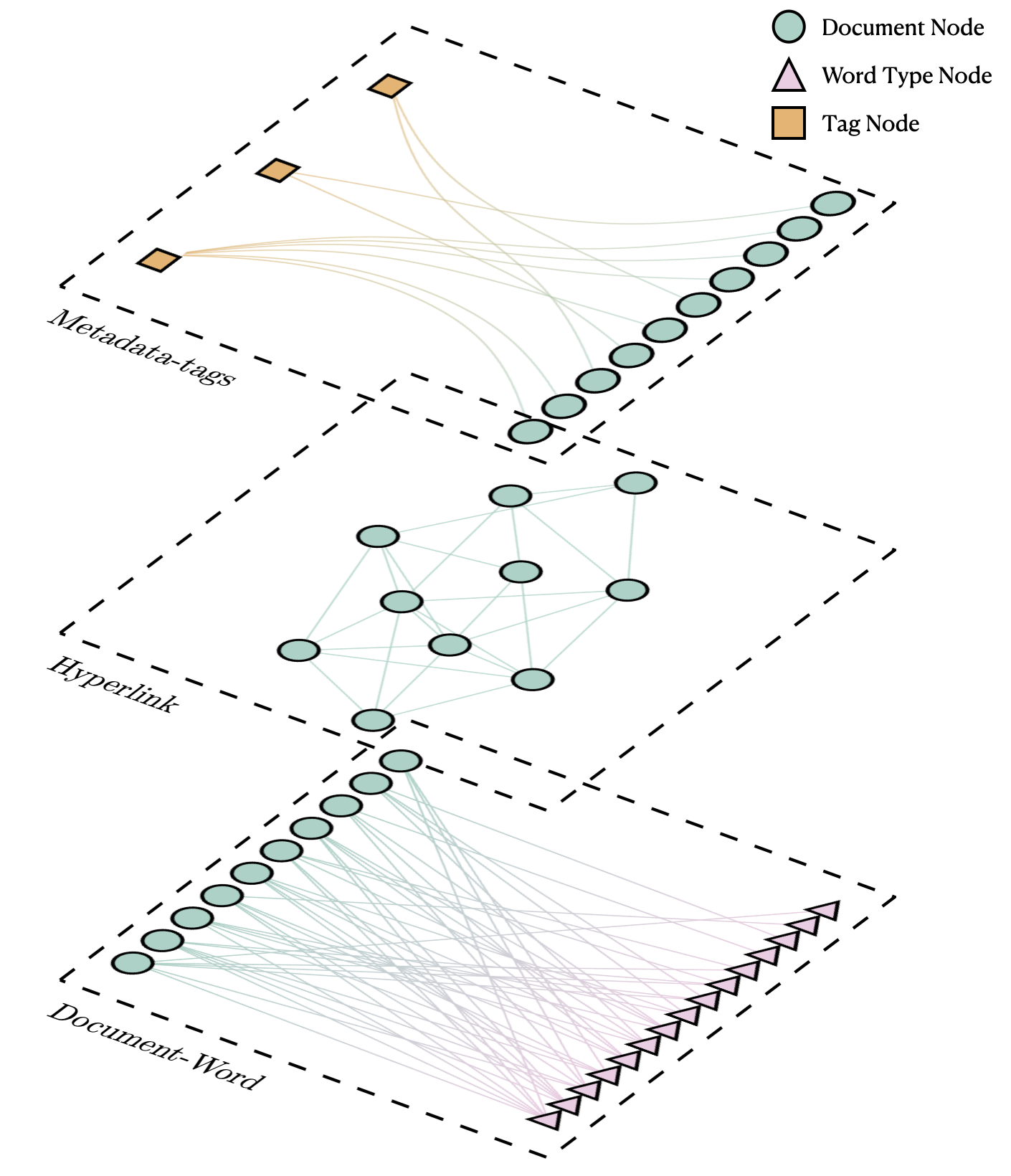
In this paper, we investigate the problem of clustering and finding topics in collections of written documents for which additional information is available as metadata and as hyperlinks between documents. We obtain a unified statistical framework to this problem by mapping it to the problem of inferring groups in multilayer networks. The key design for the unified framework proposed here is inspired by the connections [3, 13, 14, 15] between the problems of identifying (i) topics in a collection of written documents (i.e. topic modeling) [16] and (ii) communities in complex networks (i.e. community detection) [17]. In particular, Ref. [15] shows that both problems can be tackled using Stochastic Block Models (SBM) [3, 12, 18, 19, 20, 21, 28] and that SBMs, previously applied to find communities in complex networks, outperform and overcome many of the difficulties of the most popular unsupervised methods to infer structures from large collections of texts (topic modelling methods such as the Latent Dirichlet Allocation [22] and its generalizations). However, these approaches have been applied only to the textual part of collections of documents, ignoring additional information available about them. For instance, in datasets of scientific publications, one would consider only the text of the articles but not the citation networks (used in traditional community detection methods [17]) or other metadata (such as the journal or bibliographical classification)  [44, 42]. We propose here an extension of Ref. [15] and show how the diversity of information typically available about documents can be incorporated in the same framework by using multilayer SBMs [3, 10, 11]. As illustrated in Fig. 1, in addition to the bipartite Document-Word layer discussed in Ref. [15], here we incorporate a Hyperlink layer connecting the different written documents and a Metadata-Document layer that incorporates tags and other metadata. The key difference to other multilayer networks [4], as explored in Sec. 2 below, is that statistical laws [23] governing the frequency of words on documents leave fingerprints on the density of the different network layers. Our investigations in different datasets, reported in Sec. 3 for collection of Wikipedia articles and in the Supplementary Information for three other datasets, reveal that the proposed multilayer approach leads to improved results when compared to both the topic modelling approach of [15] and the usual community detection of (hyperlink) networks. Our approach leads to a more nuanced view on the communities of documents, generates a list of topics associated to the communities, and improves the link-prediction capabilities when compared to the hyperlink network alone [24]. The details on our methods can be found in the appendices, Supplementary Information, and in the repository [25].

2 Multiple data sources as multilayer networks

In this section we introduce the general methodology of our paper: we introduce the types of data we are interested in (Sec.  2.1), we show how they can be represented as a multilayer network and discuss the properties of these networks (Sec. 2.2), and we describe how they can be modelled using Stochastic Block Models (Sec. 2.3).

2.1 Setting: Multiple Data Sources

We consider a collection of $d=1,\ldots,D$ documents and we are interested in clustering and finding underlying similarities between them using combinations of the following information:

• Each document contains $k_{d}$ word tokens from a vocabulary of $V$ word types ($M=\sum_{d}k_{d}$ is the total number of word tokens).

• Documents are linked to each other by building a (directed) graph or network.

• Documents are classified by tags or other metadata.

These characteristics are typical for textual data and networks. Here we explore three types of such datasets, summarized in Tab. 1. The main dataset we use to illustrate our results was extracted from the English Wikipedia, where the documents are articles (in scientific categories), the text is the content of the articles, hyperlinks are links between articles contained in the text, and metadata are tags introduced by users to classify the articles (categories). In our main example, we selected hundreds of articles in one of three scientific categories of Wikipedia (see Appendix 1 for details). Our main findings are confirmed in a second Wikipedia dataset (obtained choosing different scientific categories), in a citation dataset (documents are scientific papers, hyperlinks are citations, the text is extracted from the title and abstract, and metadata are scientific categories), and in an E-mail dataset (documents are all E-mails from the same user, hyperlinks correspond to E-mails sent between users, and the text is the content of the E-mails). These results and further details of the data are presented in the Supplementary Information (see SI-Sec. 1).

Table 1: Summary of the datasets used in this paper.

Nodes	Wikipedia Dataset in	Wikipedia Dataset in	E-mail Dataset in	Citation dataset in
	Manuscript	SI	SI	SI
Documents	120	316	4,894	2,542
Word Types	11,545	16,344	66,088	7,677
Metadata Tags	Physics, Maths,	Statistics, Maths,	0	52 Categories
	Biology	Electrical Engineering
Edges
Hyperlinks	309	1,530	18,005	4,590
Word Tokens	155,093	321,147	761,179	116,889
Tag Labels	120	316	0	2,542

2.2 Data as Networks

The data described above can be represented as multilayer networks. The Hyperlink layer is the most obvious one, where documents are nodes and the hyperlinks are directed edges. The Metadata layer is built by a bipartite network consisting of metadata tags and documents as nodes, whereby undirected edges correspond to documents containing a given metadata-tag. Finally, the Text layer is obtained by restricting the text analysis to the level of word frequencies (bag-of-words) and then considering the bipartite network of word (types) and documents, where the edges correspond to word tokens (i.e., the count of how often a word type appears in a document). While word-nodes and metadata tags appear only in the text and the metadata layer, all layers have document nodes in common. The novelty of our multilayer approach, in comparison to other approaches using multilayer networks, is the inclusion of the text layer. The importance of using a bipartite multigraph layer [28] to represent the text, instead of alternative “word networks” [14, 26, 27], is that it contains the complete information of word occurrence in documents and allows for a formal connection to topic-modelling methods [15, 20].

Figure 2: Scaling of average degree for each class of node reveals sparse and dense layers. Scaling of the average degree $\langle k_{X}\rangle$ with the number of documents $n_{D}$ depends on the node types $X$. The average degree was computed over all nodes of the same type (see legend, where H,T,M indicates the layer) in a sample of $n_{D}$ documents from dataset. The symbols (error bars) are the average (standard deviation) over multiple random samples of documents. The prediction for the degree of word types using Eq. (1) is also plotted for reference.

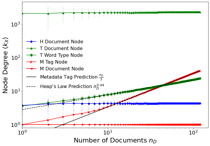
We now investigate the properties of the multilayer network described above, based on known results in networks and textual data. The most striking feature of this network is that the size of the different layers varies dramatically and scales differently with system size. A first indication of this lack of balance is seen by looking at the number of edges shown in Tab. 1: the number of edges in the text layer (i.e. word tokens) is substantially larger than the number of nodes or edges in all of the other layers. Such an imbalance is expected in all datasets in which the same type of data as outlined in Sec. 2.1 is present. To see this we investigate in Fig. 2 how the average degree $\langle k_{X}\rangle$ (number of edges/ total number of nodes) of the different node types $X$ scale with the number of documents $n_{D}$ (which plays the role of system size). For the document nodes in the Hyperlink layer and the Text layer we see a constant average degree, typical of sparse networks. The Metadata layer yields a trivial scaling linear with $n_{D}$ as in dense networks because each document has one edge to a metadata node. More interestingly, the average degree of the word type nodes in the Text layer, $\langle k_{V}\rangle$, shows a growth that scales as

$$\langle k_{V}\rangle\sim n_{D}^{\gamma},$$ (1)

with $0<\gamma<1$. This is between the usual limits expected for sparse ($\gamma=0$) and dense ($\gamma=1$) networks.

We now explain the observation in Eq. (1) in terms of properties of text in general. More specifically, the type-token relationship in texts follows Heaps’ law [29, 30, 23], which states that the number of word types $V$ scales with the word tokens $M$ as

$$V\sim M^{\beta},$$ (2)

whereby $0<\beta<1$ is the parameter of interest. The average degree is obtained as $\langle k_{V}\rangle=M/V$ and $n_{D}\propto M$ (where the proportionality constant is the average size of Wikipedia articles, in word tokens). Combining this with Eqs. (1) and (2) we obtain that $\gamma=1-\beta$. From the data used here, we estimate a Heaps’ exponent $\beta=0.56$, that leads to a prediction of $\gamma=0.44$. This prediction is shown as a dashed line in Fig. 2 and is in good agreement (for large $n_{D}$) with the average degree of word nodes.

2.3 Stochastic Block Models

To achieve our goal of clustering documents and identifying topics considering multiple type of datasets simultaneously, we need to explore statistical patterns in the connectivity of the multilayer networks discussed above. This can be obtained using Stochastic Block Models (SBMs). The choice of SBM is based on the existence of a successful computational and theoretical framework, reviewed in Ref. [12], that can be applied to networks with the characteristics needed in our problem: different types of networks (directed, bipartite, and multi edges), multilayer networks [11], and accounting for key ingredients to detect communities (e.g., degree correction and a nested/hierarchical generalizations [32]). Our previous analysis of bipartite word-document networks using this framework has outperformed traditional topic modelling approaches [15].

SBMs are a family of random-graph models that generate networks with adjacency matrix $A_{ij}$ with probability $P(\bm{A}|\bm{b})$, where the vector $\bm{b}$ with entries $b_{i}\in\{1,\cdot\cdot\cdot,B\},$ specifies the membership of nodes $i=1,\cdot\cdot\cdot,D$ into one of $B$ possible groups. For our multilayer network design – developed for the three types of data (H,T,M) as discussed in Sec. 2.2 – we fit the SBM framework to each layer combining them by constraining document groups to be the same across all layers, i.e. with a joint probability

$$P(\bm{A}_{\text{H}},\bm{A}_{\text{T}},\bm{A}_{\text{M}}|\bm{b})=P(\bm{A}_{\text{H}}|\bm{b})P(\bm{A}_{\text{T}}|\bm{b})P(\bm{A}_{\text{M}}|\bm{b}),$$ (3)

where $\bm{A}_{\text{H}}$, $\bm{A}_{\text{T}}$ and $\bm{A}_{\text{M}}$ are the adjacency matrices of each respective layer. In each individual layer, edges between nodes $i$ and $j$ are sampled from a Poisson distribution with average [20]

$$\theta_{i}\theta_{j}\omega_{b_{i},b_{j}}$$ (4)

whereby $\omega_{rs}$ is the expected number of edges between group r and s, $b_{i}$ is the group membership of node $i$, and $\theta_{i}$ is overall propensity with which a node is selected within its own group. Non-informative priors are used for the parameters $\bm{\theta}$ and $\bm{\omega}$ and the marginal likelihood of the SBM is computed as [31]

$$P(\bm{A}|\bm{b})=\int P(\bm{A}|\bm{\omega},\bm{\theta},\bm{b})P(\bm{\omega},\bm{\theta}|\bm{b})d\bm{\theta}d\bm{\omega},$$ (5)

Based on this, we consider the overall posterior distribution for a single partition conditioned the edges on all layers [35]

$$P(\bm{b}|\bm{A}_{\text{H}},\bm{A}_{\text{T}},\bm{A}_{\text{M}})=\frac{P(\bm{A}_{\text{H}}|\bm{b})P(\bm{A}_{\text{T}}|\bm{b})P(\bm{A}_{\text{M}}|\bm{b})P(\bm{b})}{P(\bm{A}_{\text{H}},\bm{A}_{\text{T}},\bm{A}_{\text{M}})}.$$ (6)

With this approach, not only the words but also the documents are now clustered into categories. We implement the inference using the package graph-tool [25, 41, 45, 43] (see SI-Sec. 2 for details and Ref. [25] for our codes).

3 Application to Wikipedia data

In this section we apply the methodology and ideas discussed above to the Wikipedia dataset which contains articles classified by users in the categories Mathematics, Physics, and Biology. We are interested in comparing the outcomes and performance of the models discussed above applied to the different types of information in the data. We fit multiple variants of the multilayer SBM, whereby we choose different layers to be included in the model.

3.1 Description Length

The performance of each model can be measured by the extent to which a model succeeds in describing (compressing) the data. This can be quantified computing its description length (DL)  [33, 34]

$$DL=-\log P(\bm{A}_{\text{H}},\bm{A}_{\text{T}},\bm{A}_{\text{M}},\bm{b}),$$ (7)

which describes the information necessary to describe both the data and the model parameters. From Eq. 6, we see that minimizing the description length is equivalent to maximizing the posterior probability $P(\bm{b}|\bm{A}_{\text{H}},\bm{A}_{\text{T}},\bm{A}_{\text{M}})$.

In Tab. 2 we summarise the DL obtained for each model in our dataset. It is quite clear that the DL of the models containing the Text layer are much larger than those containing only the Hyperlink and Metadata layers. This is a direct consequence of the large number of word types in the data, when compared to documents or hyperlinks, the lack of balance between the layers mentioned in Sec. 2.2. This lack of balance between layers thus has important consequences for the inference of partitions and our ability to compare the different models. For instance, the effectiveness of the multilayer approach could be evaluated by comparing the DL of the multilayer model (e.g., DL of model $H+T$) to the sum of the DL of the single-layer models (e.g., DL of model $H$ + DL of model $T$). In our case this comparison is not very informative because the DL of the combined model is dominated by the largest layer and the DL of the small layer often lies within the fluctuations obtained from multiple MCMC runs (see SI-Sec. 2). This reasoning suggests that the clustering of nodes would be dominated by the Text layer or, if the Text layer is excluded, by the Hyperlink layer which will dominate over the Metadata layer. However, we will see below that there are still significant and meaningful differences in the clustering of nodes obtained using different combinations of layers. This happens because the inference problem remains non-trivial because the DL landscape contains many distinct states with similar values in the DL so that even small effects due to the $H$ and $M$ layers can affect the outcome.

Table 2: Description length for each combination of layers in the multilayer stochastic block model. We compute the average description length (DL), Eq. (7), for each model class alongside the standard deviation over multiple MCMC runs. We also retrieved the minimum DL (MDL) over all the runs. The DL of the Text layer exceeds the Hyperlink and Metadata layer by several orders of magnitude, thus contributing the most to the Hyperlink + Text model.

Model	Layers	DL	MDL
H	Hyperlink	1,135 (0)	1,135
T	Text	257,775 (471)	256,973
M	Metadata	76 (0)	76
H+M	Hyperlink+Metadata	1,295 (18)	1281
H+T	Hyperlink+Text	270,230 (2,228)	267,102
H+T+M	Hyperlink+Text+Metadata	282,560 (624)	281,133

3.2 Qualitative comparison of groups of documents

(a) Wikipedia Labels

(b) Hyperlink Model, $\operatorname{\sigma}=0.0$

(c) Text Model, $\operatorname{\sigma}=0.27$

(d) Hyperlink + Text Model, $\operatorname{\sigma}=0.088$

Figure 3: Different models lead to different partitions of Wikipedia articles into communities. The network corresponds to Wikipedia articles (nodes) and hyperlinks (edges). The colour of the nodes corresponds to groups of document nodes: (a) from the Wikipedia labels (with annotations Mathematics, Physics, and Biology); (b-d) communities found from our model using different datasets (layers) and the consensus partition (see App. 2). The uncertainty $\sigma$ of the reported partitions is quantified by $0\leq\sigma\leq 1$, defined in Eq. (15) below.

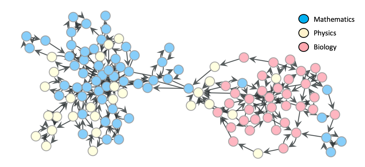
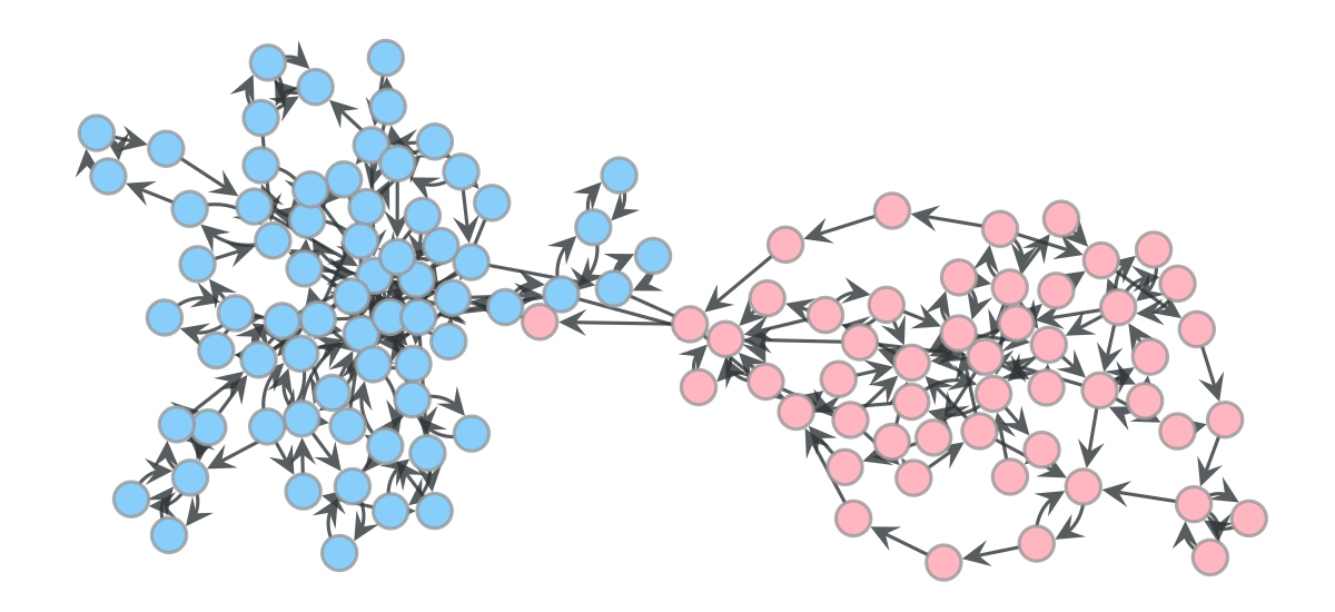
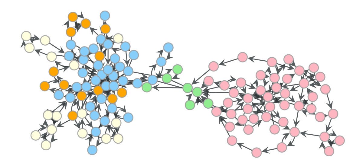
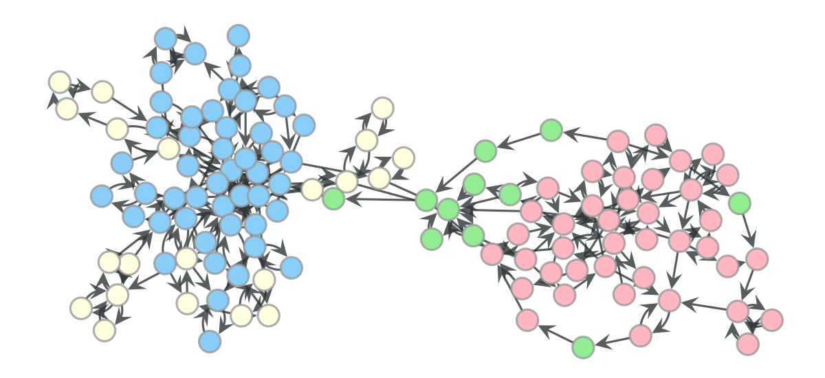
Community detection methods aim to find the partition of the nodes that best captures the structure in the network in a meaningful way whilst being robust to noise [12, 21]. We thus evaluate the different models by comparing the resulting partitioning of documents [35]. Specifically, we fit the Hyperlink, Text, and Hyperlink + Text model and obtain a best partition from combining multiple samples from the posterior $P(\bm{b}|\bm{A})$ for each model to construct a point estimate, which utilises the different parts of the posterior distribution. We then project the group membership onto the Hyperlink layer (which only contains document-nodes) and retrieve the consensus partition alongside the uncertainty of the partition [36] (see Appendix 2 for details).

Our results are shown in Fig. 3 and reveal that our model is successful in retrieving different meaningful groupings of the articles depending on the available data (i.e. layers included in the model). We first notice that the classification of articles made by users – panel (a), Wikipedia label – group articles in Mathematics and Biology that are strongly linked with each other (through hyperlinks), whereas Physics articles appear intertwined in between them. When we infer the partition of nodes based only on the hyperlink network – panel (b), Hyperlink model – we obtain that our model obtains 2 groups and it is quite confident about it (uncertainty is zero, $\sigma=0.$). This partition resembles the partition based on Wikipedia labels. When the documents are partitioned based on their text – panel (c), Text Model–, a richer picture emerges. There is a large community that resembles closely the documents classified as Biology and one of the communities obtained using the hyperlinks layer. However, the remaining documents (most of the Mathematics and Physics articles) are now grouped in $4$ categories (i.e., $5$ communities in total) which are still linked to each other but more loosely than before (even though Fig. 3 shows the Hyperlink network, the Hyperlinks were not used to group documents in panels a) and c)). Finally, when hyperlinks and text are used simultaneously – panel (d) – $4$ communities are found, which resemble the previous ones but that also show important distinctions. This demonstrates that even if the Text layer dominates the description length, there are noticeable differences in the inferred partitions when using the hyperlinks in addition to text for clustering documents.

We now argue that the more nuanced classification of documents obtained with the Text and Hyperlink + Text models are qualitatively meaningful. For example, we can see a cluster of 5 (Physics) nodes in the bottom left of the Hyperlink model that was not identified as a separate group, but it is now picked up in the Text and Hyperlink + Text model. This cluster of nodes include Wikipedia articles on the Josephson effect, macroscopic quantum phenomena, magnetic flux quantum, macroscopic quantum self trapping, and quantum tunnelling. Even more strikingly, in the bottom of the network there is a lone (Physics) green node surrounded by (Biology) red nodes which corresponds to the Wikipedia article on isotopic labelling (a technique in the intersection of Physics and Biology). In traditional community detection methods, which use link information as an indicator of groups, such a node would be in the community of its surrounding neighbours. However, in the Hyperlink + Text model, we are able to detect the uniqueness of such a node.

3.3 Quantitative comparison between different models

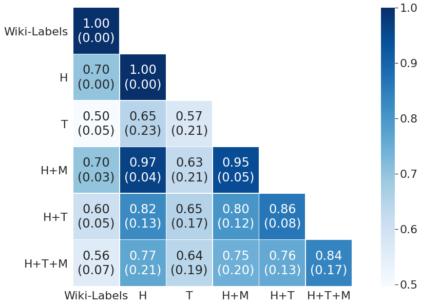
In the example discussed above it was clear that the different models yielded different yet related partitions of Wikipedia articles. In order to quantify the similarity of the results of the different models, we performed a systematic comparison of the partitions generated by multiple runs of each model and computed their similarities using the maximum overlap partition (Fig. 4, see Appendix 2 for details). The results show that the partitions generated by the Hyperlink + Text model is most similar to the Text model. Similar results are obtained in our alternative datasets – see SI-Sec. 1 – and using the normalised mutual information (NMI) as an alternative dissimilarity measure –see SI-Sec. 3.

Figure 4: Maximum partition overlap of the consensus partitions between the model classes. The average and standard deviations of the maximum partition overlap between and within different models.

We also compare the Hyperlink and Hyperlink + Text model in terms of their ability to predict missing edges [24, 37] (see Appendix 3 for details on our method). We found that the Hyperlink+Text model has an Area-Under-Curve (AUC) score of $0.63\pm 0.06$ (average $\pm$ standard deviation) and the Hyperlink model has $0.54\pm 0.02$, with the difference being statistically significant ($p=0.0013$, using a 2-sample t-test). This confirms that the multilayer approach proposed here is successful in retrieving existing relationships that are missed in the network-only approach.

3.4 Lack of balance in the Hyperlink-Text model

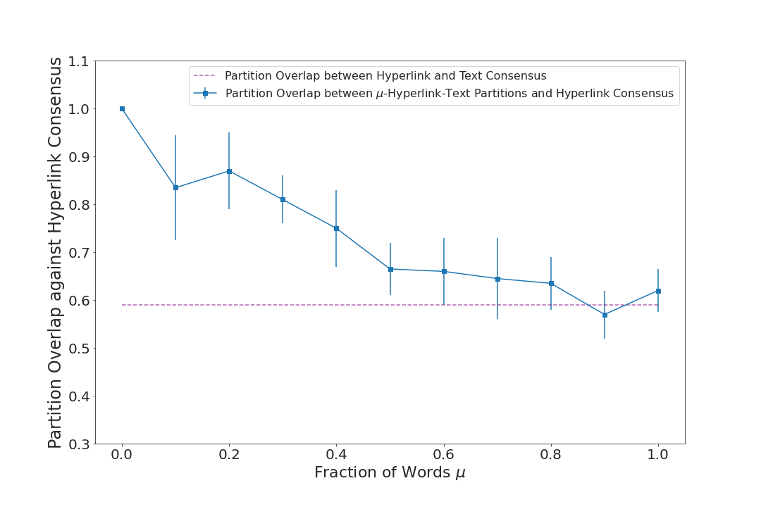
The results of the previous sections are strongly influenced by the lack of balance in Hyperlink + Text model, as discussed in Sec. 2. To further illustrate this point, here we artificially reduce the unbalance of the multilayer network by sampling a fraction $\mu$ of word tokens before fitting a Hyperlink + Text model. We expect that, as we increase the fraction of words $\mu$, the Text layer will increasingly dominate the inference. This expectation is confirmed in Fig. 5, which shows that for $\mu\geq 0.6$, the partition overlap of the $\mu-$hyperlink-text model is statistically indistinguishable from the partition overlap obtained using the Text-only model. That is, we see that the Text layer dominates the inference in the $\mu-$Hyperlink + Text for $\mu\geq 0.6$. However, as discussed above, the effect of the hyperlink layer can lead to different consensus partition.

Figure 5: Text layer determines the partitions obtained in the multilayer model (Hyperlink + Text). Similarity (overlap of consensus partition) between Hyperlink partition and $\mu$-Hyperlink-Text partition as a function of the subsampling parameter $\mu$ where $\mu=0$ ($\mu=1$) corresponds to the case with all (none) of the word tokens removed in the Hyperlink-Text model. For a given value of $\mu$, a random fraction $1-\mu$ of the words were removed and the Hyperlink + Text model was then fitted for multiple iterations. The consensus partition was then computed for the Hyperlink + Text model and its partition overlap with Hyperlink model. A higher sub-sampling of text (i.e. smaller values of $\mu$) results in the consensus partition between the Hyperlink + Text and Hyperlink model having a high degree of overlap.

3.5 Topic Modelling: Groups of Words

Since our approach provides a clustering of all nodes, we not only group documents but also words. The groups of word (types) can be interpreted as the topics of the documents linked to them, showing that our framework simultaneously solves the traditional problem of topic modeling [22, 14]. Below we show the topics obtained in our Wikipedia dataset, as an example of our generic topic-modelling methodology.

In the consensus partition of the Hyperlink-Text network (see Fig. 3) we found 12 topics (groups of word types). The most frequent words in each of these topics is shown in Tab. 3. Qualitatively, we see that topics are often composed of semantically related words, e.g. topics 1 and 3 contain a large number of key words associated to Biology whilst topics 5 and 10 contains a large number of jargon related to Physics.

We now discuss the topical composition of (groups of) documents. Let $T=B_{V}$ be the number of topics and $B_{D}$ be the number of document groups, then the mixture proportion of topic $t=1,\ldots,T$ in document group $i=1,\ldots,B_{D}$ is given by

$$f_{i}^{t}=\frac{n_{i}^{t}}{\sum_{t^{\prime}=1}^{T}n_{i}^{t^{\prime}}},$$ (8)

where $n_{i}^{t}$ is the number of word tokens in topic $t$ that appeared in documents $d$ in document-group $i$. The results obtained for the four document groups are shown at the bottom of Tab. 3. Interestingly, topic $4$ cannot be identified with any specific group of documents. This suggests that the words in this topic are similar to so-called stopwords, a pre-defined set of common words considered uninformative which are typically removed from the corpus before any model is to be fitted in order to improve the model [38]. This is consistent with the finding of Ref. [15] that SBMs applied to word-document networks were able to automatically filter stop words by grouping them into a “topic” that is well connected to all documents. Our findings suggest that the same is true for multilayer models and that our approach is robust against the presence of stopwords. In fact, this stopword topic is responsible for a large fraction ($40\%$) of the topic-proportion for all groups of documents. The underlying reason for this is the higher frequency of these words, which (due to Zipf’s law) dominate the weights of the topic mixture models  [46]. To overcome this feature, and assess the over- or under-representation of topics more rigorously, we account for the overall frequency of occurrence of words in topics $t$ as

$$\langle f^{t}\rangle=\frac{\sum_{i=1}^{B_{D}}n_{i}^{t}}{\sum_{t=1}^{T}\sum_{j=1}^{B_{D}}n_{j}^{t}},$$ (9)

and define the normalised value of the mixture proportion of topic $t$ in document group $i$ as

$$\tau_{i}^{t}=\frac{f_{i}^{t}-\langle f^{t}\rangle}{\langle f^{t}\rangle}.$$ (10)

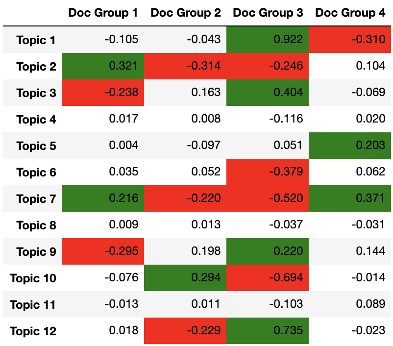
This normalised measure has an intuitive interpretation: $\tau_{i}^{t}>0$ ($\tau_{i}^{t}<0$) implies that topic $t$ is over-represented (under-represented) in document group $d$. In Fig. 6, we show $\tau_{i}^{t}$ for the 12 topics and the 4 document groups, providing a much clearer view on the connection between topics and groups of documents. For example, we see that document group 2 (articles labelled as Physics) has a large over-representation of topic 10, which corresponds to the Physics topic whilst being underrepresented in document group 2 (articles labelled as Biology). Looking at the model’s newly proposed document group (group 4) we see that it has an over-representation from topics 7 and 5 (and in a less extent from topics 2, 9, and 11), confirming its hybrid category.

Table 3: Groups of word types as topics. Upper table: the $20$ most frequent words in the 12 topics (word groups) found in the consensus partition of the Hyperlink + Text model. Lower table: the topic proportion (8) of the four groups of documents.

Group

Topic 1

Topic 2

Topic 3

Topic 4

Topic 5

Topic 6

Topic 7

Topic 8

Topic 9

Topic 10

Topic 11

Topic 12

occur

chemical

protein

one

system

group

transform

action

happen

quantum

every

factor

specific

loop

cell

also

time

space

law

translation

frequency

equation

basis

expression

within

electron

site

use

state

define

critical

class

fast

transformation

unique

region

process

transition

activity

form

work

field

magnetic

line

output

theorem

degree

molecular

produce

chemistry

pathway

function

second

point

matter

measure

input

symmetry

positive

sequence

increase

atom

cellular

give

effect

theory

scale

central

algorithm

dimension

open

information

mechanism

stable

organism

two

phase

value

plane

primary

digital

denote

close

end

cause

ion

amino

may

interaction

product

spectrum

unknown

classical

fix

molecule

acid

pattern

enzyme

however

potential

constant

volume

interior

let

reference

domain

target

crystal

synthesis

example

could

vector

temperature

surface

mechanic

exact

signal

step

reach

species

result

derive

physic

axis

side

coordinate

closed

alternative

bind

prediction

tissue

call

difference

physical

statistical

center

lie

restrict

bond

gene

label

proteins

first

full

energy

sign

flow

real

picture

family

control

compound

cancer

different

free

element

effective

copy

mathematics

infinitesimal

interact

human

reaction

activate

know

hold

particle

symbol

block

geometry

index

cycle

encode

crystallography

genetic

make

observe

parameter

speed

configuration

operator

interpretation

biological

body

oxygen

membrane

number

research

whose

electric

read

differential

formulate

life

dna

solid

release

structure

propose

mathematical

equilibrium

alternate

representation

equivalently

translate

rate

unstable

mutation

show

year

linear

unchanged

table

invariant

maximal

structural

formation

atomic

regulation

include

paper

matrix

assumption

transport

generalize

scheme

biology

1 (Mathematics)

0.1481

0.0213

0.0444

0.400

0.0578

0.0722

0.0510

0.0127

0.00163

0.147

0.0105

0.0338

2 (Physics)

0.138

0.0409

0.0291

0.404

0.0643

0.0710

0.07940

0.0127

0.0009583

0.105

0.0102

0.0445

3 (Biology)

0.297

0.0234

0.0536

0.351

0.0673

0.0426

0.0313

0.0121

0.00166

0.0347

0.00929

0.0759

4 (New Group)

0.107

0.0342

0.0355

0.405

0.0771

0.0728

0.0895

0.0122

0.00156

0.112

0.0113

0.0428

Figure 6: Normalised contribution of topics to the group of documents. The normalized measure (10) was computed for all 4 document groups and 12 word groups (topics). We set a threshold of $\tau_{i}^{t}\geq 0.2$ ($\tau_{i}^{t}\leq-0.2$) to define if a topic is over- (under-) represented in a document group $d$.

4 Discussion and Conclusions

In this paper, we introduced and explored a formal methodology that combines multiple data types (e.g., text, metadata, links) to perform the common tasks of clustering and inferring latent relationships between documents in text analysis. The main theoretical advantage of our methodology is that it incorporates all the different types of data into a single, consistent, statistical model. Our approach is based on an extension of multilayer Stochastic Block Models, that have been used previously to find communities in (sparse) complex networks and that is used here to perform text analysis (see Refs. [3, 18] for alternative uses of SBMs for topic modelling). On the one hand, our method extends community-detection methods to the analysis of text in the presence of multiple data types, our main finding being that: (i) universal statistical properties of texts lead to different link densities at the different layers of the network; and (ii) that the word layer plays a dominant role in the inference of partitions. On the other hand, our method can be viewed as a generalized topic modelling method that incorporates meta-data and hyperlinks, labels the communities of documents by examining the proportion of topics, and builds on the previous connections between SBMs and Latent Dirichlet Allocation [15, 20].

Our investigations on four different datasets show consistent results that reveal the potential and limitations of our approach. Our most important finding is that our methodology succeeds in using the multiple data types (e.g., a text layer) leading to more nuanced communities of documents and in increasing the ability to predict missing links. On the practical side, the lack of balance between the different layers poses challenges on how to evaluate the contributions of different layers because the description length obtained in the inference process is dominated by the text layer and variations obtained within the (Monte Carlo) inference process become larger than the contribution of alternative layers. This suggests further investigations on the role of unbalanced layers in multilayer networks, and how to deal with them within the proposed framework, as important steps to expand the success of complex-network methods to other classes of relevant datasets.

Appendix

Appendix 1: Wikipedia Data Collection and Preparation

We used a snapshot of the Wikipedia data retrieved on the 5th of June, 2020. The following lists the data extraction and processing steps:

1. Data Retrieval: We retrieved the Wikipedia articles and their content (metadata, text, link) through the MediaWiki API. and parsing the Wikipedia dumps.

2. Network Formulation: We constructed a network whereby each node represents a Wikipedia article and each (directed) edge represents hyperlinks between the Wikipedia articles. We removed any nodes with less than 2 outgoing links.

3. Retrieve Connected Component: For ease of analysis, we extracted the largest connected component in the hyperlink network constructed.

4. Text Processing: We process the Wikipedia text data through both tokenization and lemmatization using NLTK [40].

The resultant dataset is available in our repository [25].

Appendix 2: Maximum Overlap and Consensus Partition

The maximum overlap between partitions measures the similarities between sets of partitions. The maximum overlap between partitions $\bm{x}$ and $\bm{y}$ is given by

$$w(\bm{x},\bm{y})=\operatorname*{arg\,max}_{\bm{\mu}}\sum_{i}\delta_{x_{i},\mu(y_{i})},$$ (11)

where $\bm{\mu}$ is a bijective mapping between the group labels [36].

The normalized maximum overlap between partitions $\bm{x}$ and $\bm{y}$ is given by

$$w(\bm{x},\bm{y})=\frac{\sum_{i}\delta_{x_{i},y_{i}}}{N},$$ (12)

where N is the number of nodes and lies in the unit interval [0,1].

Given multiple partitions, we also wish to extract a consensus partition $\hat{\bm{b}}$ which has the maximal sum of overlaps with all the partitions. Such a consensus partition can be obtained through the double maximization of the set of equations:

$$\hat{b}_{i}=\operatorname*{arg\,max}_{r}\sum_{m}\delta_{\mu_{m}(b_{i}^{m}),r}$$ (13)

$$\bm{\mu}_{m}=\operatorname*{arg\,max}_{\bm{\mu}}\sum_{r}m_{r,\mu(r)}^{(m)},$$ (14)

where $\bm{\mu}$ is a bijective mapping between the group labels and $m_{r,\mu(r)}^{(m)}$ is the contingency table between $\hat{\bm{b}}$ and partition $\bm{b}^{(m)}$. An iterative procedure is then carried out on the set of equations until no further improvement is possible. The uncertainty $\sigma$ of the consensus partition obtained from $M_{p}$ partitions can be quantified as [36, 25]

$$\sigma=1-\frac{1}{NM_{p}}\sum_{i}\sum_{m}\delta_{\mu_{m}(b_{i}^{m}),\hat{b}_{i}}.$$ (15)

Appendix 3: Supervised Learning Via Link Prediction

A supervised learning approach to select the best model can be done through the task of link prediction [37, 39]. Let $\bm{A}^{O}$ be the observed network and $\delta\bm{A}$ be missing or spurious edges. The desired posterior distribution of missing entries $\delta\bm{A}$ conditioned on the observed network $\bm{A}^{O}$ can be computed as

$$P(\delta\bm{A}|\bm{A}^{O})=\frac{\sum_{\bm{b}}P(\bm{A}^{O}\cup\delta\bm{A}|\bm{b})P(\bm{b}|\bm{A}^{O})}{P(\bm{A}^{O}|\bm{b})}.$$ (16)

However, as the normalization constant is difficult to obtain, the numerator of Eq. 16 can be computed by sampling partitions from the posterior and then inserting or deleting edges from the graph and computing the new likelihood. As a result, we therefore may compute the relative probability between specific sets of alternative predictive hypotheses $\{\delta\bm{A}_{i}\}$ through the likelihood ratios ratio

$$\lambda_{i}=\frac{P(\delta\bm{A}_{i}|\bm{A}^{O})}{\sum_{j}P(\delta\bm{A}_{j}|\bm{A}^{O})}.$$ (17)

We can compute the area under curve (AUC) of the receiver operating characteristic curve to evaluate the SBM’s classification abilities. Furthermore, given two sets of AUCs from two different models, we can compare the models’ performance by computing the t-statistic for a null model with zero mean for the difference in AUC which is given by

$$t_{\Delta AUC}=\frac{\langle\Delta AUC\rangle}{\sigma_{\Delta AUC}/\sqrt{n}},$$ (18)

where $\langle\Delta AUC\rangle$, $\sigma_{\Delta AUC}$, and n are the mean, standard deviation and size of the population.

Additional Material

The supplementary Material is available at https://epjdatascience.springeropen.com/articles/10.1140/epjds/s13688-021-00288-5#Sec16. Codes and data are available at https://topsbm.github.io.

References

- [1] B. Kedem, V. De Oliveira, and M. Sverchkov, Statistical Data Fusion, World Scientific , 200 Pages, (2017)
- [2] F. Costanedo, A Review of Data Fusion Techniques, The Scientific World Journal, ID. 704504, 19 Pages, (2013)
- [3] Y. Zhu, X. Yan, L. Getoor, and C. Moore, Scalable text and link analysis with mixed-topic link models, Proceedings of the 19th ACM SIGKDD International Conference on Knowledge Discovery and Data Mining, 473–481, (2013)
- [4] M. Kivelä, A. Arenas, M. Barthelemy, J. Gleeson, Y. Moreno, and M. Porter, Multilayer Networks, Journal of Complex Networks, Vol. 2, Issue 3, (2014)
- [5] M. Zanin, D. Papo,P. A. Sousa, E. Menasalvas, A. Nicchi, E. Kubik, and S. Boccaletti, Combining complex networks and data mining: Why and how, Physics Reports, Vol. 635 (2016)
- [6] E. Breck, M. Zinkevich, N. Polyzotis, S. Whang and S. Roy, Data Validation for Machine Learning, Proceedings of SysML, (2019)
- [7] K. O’Leary and M. Uchida, Common problems with Creating Machine Learning Pipelines from Existing Code, Third Conference on Machine Learning and Systems (MLSys), (2020)
- [8] R. Arun, V. Suresh, C. E. V. Madhavan, and M. N. N. Murthy, On finding the natural number of topics with latent dirichlet allocation: Some observations, Advances in Knowledge Discovery and Data Mining, pg. 391-402 (2010)
- [9] J. Cao, T. Xia, J. Li, Y. Zhang, and S. Tang, A density-based method for adaptive LDA model selection, Neurocomputing, Vol. 72, pg. 1775–1781 (2009)
- [10] T. Vallès-Català, F. A. Massucci, R. Guimerà, and M. Sales-Pardo, Multilayer Stochastic Block Models Reveal the Multilayer Structure of Complex Networks, Physical Review X, Vol. 6, pg. 011036 (2016)
- [11] T. P. Peixoto, Inferring the mesoscale structure of layered, edge-valued and time-varying networks, Physical Review E 92 (4), 042807, (2015)
- [12] T. P. Peixoto, Bayesian stochastic blockmodeling, Advances in Network Clustering and Blockmodeling, ch. 11, (2019)
- [13] B. Ball, B. Karrer, and M. E. J. Newman, Efficient and principled method for detecting communities in networks, Phys. Rev. E 84, 036103 (2011)
- [14] A. Lancichinetti, M. I. Sirer, J. X. Wang, D. Acuna, K. Körding, and L. A. N. Amaral, High-Reproducibility and High-Accuracy Method for Automated Topic Classification, Physical Review X, 5(1), 011007 (2015)
- [15] M. Gerlach, T. P. Peixoto, and E. G. Altmann, A network approach to topic models, Sci. Adv. 4, eaaq1360 (2018)
- [16] D. M. Blei, Probabilistic Topic Models, Communications of the ACM, Vol. 55, (2012)
- [17] S. Fortunato, Community detection in graphs, Physics Reports, Vol. 486 Issue 3-5, Page 75-174, (2010)
- [18] C. Bouveyron, P. Latouche, and R. Zreik, The stochastic topic block model for the clustering of vertices in networks with textual edges, Statistics and Computing, 1–21 (2016)
- [19] P. W. Holland, K. B. Laskey, and S. Leinhardt, Stochastic blockmodels: First steps, Social Networks, Vol. 5, Issue .2, (1983)
- [20] B. Karrer and M. E. J. Newman, Stochastic blockmodels and community structure in networks, Physical Review E 83, 016107, (2011)
- [21] M. Hastings, Community Detection as an Inference Problem, Physical review. E, Statistical, nonlinear, and soft matter physics, Vol. 74, pg. 035102 (2006)
- [22] D. M. Blei, A. Y. Ng, and M. I. Jordan, Latent Dirichlet Allocation, The Journal of Machine Learning Research, Vol. 3, (2003)
- [23] E. G. Altmann and M. Gerlach, Statistical laws in linguistics, Creativity and universality in language, pg. 7-26, (2016)
- [24] R. Guimera and M. S. Pardo, Missing and spurious interactions and the reconstruction of complex networks, Proceedings of the National Academy of Sciences, Vol. 106, pg. 22073 –22078 (2009)
- [25] Codes: TopSBM (Topic Models based on Stochastic Block Models, https://topsbm.github.io) and graph-tool (Efficient network analysis, https://graph-tool.skewed.de)
- [26] H. F. de Arruda, L. D. F. Costa, and D. R. Amancio, Topic segmentation via community detection in complex networks, Chaos , 26(6), 063120 (2016)
- [27] L. Leydesdorff and A. Nerghes, Co-word Maps and Topic Modeling: A Comparison Using Small and Medium-Sized Corpora (N 1,000), Journal of the Association for Information Science and Technology, Vol. 68, Issue 4, (2017)
- [28] T.-C. Yen, D. B. Larremore. Community Detection in Bipartite Networks with Stochastic Blockmodels, Physical Review E, 102, 032309 (2020).
- [29] G. Herdan, Type-token mathematics, Mouton (1960)
- [30] H. S. Heaps, Information Retrieval, New York: Academic (1978)
- [31] T. P. Peixoto, Nonparametric Bayesian inference of the microcanonical stochastic block model, Physical Review E 95 (1), 012317, (2017)
- [32] T. P. Peixoto, Hierarchical block structures and high-resolution model selection in large networks, Physical Review X 4 (1), 011047, (2014)
- [33] J. Rissanen, Modeling by shortest data description, Automatica, Vol. 14, pg. 465–471 (1978)
- [34] P. Grünwald, The Minimum Description Length Principle, MIT Press (2007)
- [35] D. Hric, R. K. Darst, and S. Fortunato, Community detection in networks: Structural communities versus ground truth, Physical Review E 90, 062805 (2014)
- [36] T. P. Peixoto, Revealing consensus and dissensus between network partitions, Phys. Rev. X 11, 021003 (2021).
- [37] T. Vallès-Català, T. P. Peixoto, R. Guimerà, and M. Sales-Pardo, Consistencies and inconsistencies between model selection and link prediction in networks, Phys. Rev. E 97 062316 (2018)
- [38] E. Haddi, X. Liu, and Y. Shi, The Role of Text Pre-processing in Sentiment Analysis, Procedia Computer Science, Vol. 17, (2013)
- [39] A. Clauset, C. Moore, and M. E. J. Newman, Hierarchical structure and the prediction of missing links in networks, Nature, Vol. 453, pg. 98-101 (2008)
- [40] S. Bird, E. Loper, and E. Klein Natural Language Processing with Python, O’Reilly Media Inc. (2009)
- [41] T. P. Peixoto, Efficient Monte Carlo and greedy heuristic for the inference of stochastic block models, Physical Review E 89 (1), 012804, (2014)
- [42] M. Newman and A. Clauset, Structure and inference in annotated networks, Nature Communications, Vol. 7 (2015)
- [43] M. E. J. Newman and G. T. Barkema, Monte Carlo Methods in Statistical Physics, Oxford University Press (1999)
- [44] D. Hric, T. P. Peixoto and S. Fortunato, Network structure, metadata, and the prediction of missing nodes and annotations, Phys. Rev. X 6 3, 031038 (2016)
- [45] T. P. Peixoto, Merge-split Markov Chain Monte Carlo for community detection, Phys. Rev. E 102, 012305 (2020).
- [46] E. G. Altmann, L. Dias, and M. Gerlach, Generalized entropies and the similarity of texts, Journal of Statistical Mechanics: Theory and Experiment, Vol. 2017, Issue 1, pg 014002, (2017)