Pilot Assignment for Joint Uplink-Downlink Spectral Efficiency Enhancement in Massive MIMO Systems with Spatial Correlation
Abstract
This paper proposes a flexible pilot assignment method to jointly optimize the uplink and downlink data transmission in multi-cell Massive multiple input multiple output (MIMO) systems with correlated Rayleigh fading channels. By utilizing a closed-form expression of the ergodic spectral efficiency (SE) achieved with maximum ratio processing, we formulate an optimization problem for maximizing the minimum weighted sum of the uplink and downlink SEs subject to the transmit powers and pilot assignment sets. This combinatiorial optimization problem is solved by two sequential algorithms: a heuristic pilot assignment is first proposed to obtain a good pilot reuse set and the data power control is then implemented. Numerical results manifest that the proposed algorithm converges fast to a better minimum sum SE per user than the algorithms in previous works.
Index Terms:
Massive MIMO, Max-Min Fairness Optimization, Pilot Assignment.I Introduction
Massive multiple input multiple output (MIMO) is a key component of 5G since this technology can improve ergodic spectral efficiency (SE) with the orders of magnitude compared to single-antenna systems. It is achieved by equipping each base station (BS) with a large number of antennas such that the system can spatially multiplex tens of users at the same time and frequency resource [1, 2]. The quasi-orthogonality of all channels allows a simple linear beamforming to yield SE close to the channel capacity for single-cell systems, in which orthogonal pilot signals are assumed to be available for all users. In cellular Massive MIMO systems, it is an impractical assumption because the pilot overhead is directly proportional to the total number of users [3], while the coherence interval is limited. A small set of orthogonal pilot signals should be reused among the cells, which results in mutually correlated interference known as pilot contamination that downgrades the ergodic SE [4].
In order to mitigate pilot contamination, an observation is that some users will cause more severe contamination to each other when they use the same pilot. This issue should be avoided in the pilot assignment. The system can reuse pilot signals in a way that gives these users a priority to use orthogonal pilots. Nonetheless, an optimal pilot assignment is expensive to find since it is attained by solving a combinatorial problem. Heuristic algorithms with affordable complexity are necessary in practice to eliminate pilot contamination at a reasonable cost. It should be noticed that most previous works only consider the pilot assignment for either the uplink or downlink transmission, see [3, 5] and references therein. The authors [6] were the first to propose a heuristic pilot assignment algorithm taking both uplink and downlink into account, but based on the asymptotic SE from uncorrelated Rayleigh fading that behaves differently from the capacity regime for a limited number of BS antennas and spatially correlated channels. Meanwhile, the combinations of pilot signals to obtain the pilot assignment increases rapidly with the total number of users in all cells making it an intractable solution. Motivated by the fact that uncorrelated channels rarely appear in practice [7], the pilot assignment for spatially correlated channels were considered in [3, 8], but the pilot assignment for jointly enhancing the uplink and downlink SE has not been considered in this context.
In this paper, we assign the pilot signals to jointly maximize the minimum weighted sum of uplink and downlink SE per user with spatially correlated channels. This optimization problem has flexibility since the weights can be used to assign different priorities to the downlink and uplink. The optimization problem is based only on statistical channel information, thus the obtained solution can be utilized as long as the statistics remain the same. Since this optimization problem is combinatorial and NP-hard, we propose a heuristic pilot assignment that works well for systems with a limited number of BS antennas. The obtained pilot assignment solution outperforms the other benchmarks from previous works.
Notation: The upper and lower-bold letters denote vectors and matrices, respectively. The notation is the Hermitian transpose. is the expectation of a random variable, while denotes circularly complex Gaussian distribution. The identity matrix of size is denoted by . Finally, is the trace operator, is Euclidean norm, and denotes the big- notation.
II System Model
We consider a multi-cell Massive MIMO system comprising cells, each with an -antenna BS serving single-antenna users. The system uses a time-division duplexing protocol. Let be the length of each coherence block whereof symbols are used for the uplink training and the remaining is used for the data transmission. We denote by and the fraction of the symbols used for the uplink and downlink data transmission and satisfied . The set contains all tuple of cell and user indices in the system as
| (1) |
The channel between user in cell and BS is denoted as and is assumed to feature correlated Rayleigh fading: , where is the channel correlation matrix. All BSs know the channel statistics, but need to estimate the realizations in each coherence block.111For sake of the simplicity, we assume that the channel correlation matrices are known. In practical systems, we can easily estimate the channel correlation matrices by averaging over many different instantaneous channel realizations.
II-A Uplink training phase
Let us introduce a set of mutually orthogonal pilot signals, reused among the users. The pilot signal assigned to user in cell is denoted as . In the uplink training phase, the received baseband pilot signal at BS is
| (2) |
where is an noise matrix with independent elements distributed as and being the noise variance in the uplink. The channel estimate of is obtained from (2) by MMSE estimation [4] as
| (3) |
where is given as
| (4) |
For all the channel estimates are distributed as
| (5) |
The channel estimate in (3) together with its statistical information in (5) are used to formulate the linear processing vectors for the data transmission and compute closed-form ergodic SE expressions for each user.
II-B Data transmission
In the uplink data transmission, the users in each cell simultaneously send data to the serving BS. Specifically, user in cell sends a complex data symbol with . The received signal at BS is
| (6) |
where is the transmit data power and is the uplink Gaussian noise with . We assume BS detects the desired signal from its user by utilizing a maximum-ratio combining vector as
| (7) |
The desired signal is then obtained from
| (8) |
In the downlink data transmission, BS transmits a signal to its users, which is formulated as
| (9) |
where is the power allocated to the data symbol with . The maximum ratio (MR) precoding vector
| (10) |
is used. The received signal at user in cell is a superposition of the signals from all BSs as
| (11) |
where denotes the additive noise which is distributed as and is the noise variance in the downlink. By applying the standard Massive MIMO methodology [4] to (8) and (11), the closed-form expression of the ergodic uplink and downlink SEs in Lemma 1 are attained.
Lemma 1.
Closed-form expression of the uplink and downlink ergodic SEs of user in cell are respectively
| (12) | ||||
| (13) |
| (14) |
| (15) |
Proof.
The proof follows along the lines of Corollaries 4.5 and 4.9 in [4] except for the different notations and the fact that pilot reuse pattern is arbitrary and not defined in advance. ∎
In the SINR expressions, the numerator represents an array gain as the trace of the covariance matrix is proportional to the number of BS antennas. The first term of the denominator represents coherent interference originating from pilot contamination caused by the pilot reuse and it grows with the number of BS antennas. The last terms of the denominator are noncoherent interference and noise. While the uplink SINR expression of each user only depends on the channel estimate of this own user, a superposition of the channel estimation quality from all the users are observed in the downlink SINR expression. The denominators of the SINR expressions in (14) and (15) indicate the different contributions of a pilot reuse pattern to the uplink and downlink data transmission. The coupled nature motivates a pilot assignment for jointly optimizing the both SEs per user instead of either the uplink or downlink SE as in most previous works.
III Max-Min Fairness Optimization
This section studies the pilot assignment for the weighted max-min sum SE per user fairness problem with uplink and downlink transmit power constraints. Due to the inherent non-convexity, we propose a heuristic algorithm to obtain a good local solution with tolerable computational complexity.
III-A Problem formulation
By introducing the weights that prioritize the uplink and downlink transmission of arbitrary user in cell , the optimization problem is formulated for a given set of orthogonal pilot signals as
| (16a) | ||||
| subject to | (16b) | |||
| (16c) | ||||
where is the maximum power that each user and BS can allocate to in the uplink and downlink, respectively. Problem (16) is combinatorial and its optimal solution for the pilots is obtained by exhaustive search over possible pilot assignments. For the pilot length of , there are different pilot assignments, which is impossible to perform in a large-scale system [3]. We notice that by introducing weights and considering spatially correlated fading, problem (16) is a generalization of previous works which only focus on uncorrelated Rayleigh channel for either the uplink or downlink transmission [9].
III-B Heuristic pilot assignment with fixed data powers
A low-complexity heuristic pilot assignment algorithm is proposed, in which the user having the lowest weight sum SE is prioritized. For a given set of transmit power coefficients, problem (16) becomes
| (17) |
We assume that all users first randomly select the pilot signals such that there is no pilot contamination inside a cell. After that, cell reallocates the pilot signals to its users with the availability of pilot assignment information from other cells. If we define the weighted sum SE of user in cell as
| (18) |
then BS can sort all users in the ascending order as
| (19) |
where is a permutation of the set . From these notations, user in cell has the weighted sum SE .
We now compute the normalized mean square error (NMSE) of user in cell as
| (20) |
then the channel estimation quality of the users in cell is sorted in the ascending order as
| (21) |
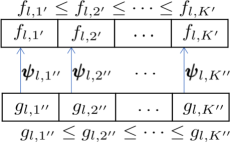
where is a permutation of the set . The pilot signal currently used by user is reassigned to user . The intuition is to dedicate pilots signal subject to less pilot contamination to users with worse conditions, which is viewed as one with a smaller . Our proposed pilot assignment for users in cell is illustrated in Fig. 1. This process is implemented cell-by-cell in an iterative algorithm (please see Algorithm 1). Concerning on the per-cell-based pilot assignment, a new pilot reuse set may harm the minimum weighted sum SE in the entire system. To avoid this issue, we introduce a backtracking condition to assign the pilot signals at iteration as in Lemma 2.
Lemma 2.
If the pilot signals are only assigned to the users in cell when the objective function in (17) does not increase, then the proposed iterative pilot assignment approach converges to a fixed point.
Proof.
Let us denote and as the minimum weighted sum SE per user before and after BS reassigns the pilot signals, i.e.,
| (22) | |||
| (23) |
where and are the uplink and downlink SEs at iteration and , respectively. A criterion is then used to approve if the reassignment is valid by checking the backtracking condition
| (24) |
which ensures a nondecreasing objective function in problem (17). We stress that the condition (24) needs to be implemented in each iteration due to the non-convexity of (22) and (23). Moreover the limited power budgets in (16b) and (16c) ensure that this objective function is bounded from above for any set of pilot and data power coefficients in the feasible domain. Consequently, problem (17) converges to a fixed point and we conclude the proof. ∎
During assigning the pilot signals to the users over cells, the proposed approach will be stopped when, for example, a small variation of two consecutive iterations, which is computed for all the cells as
| (25) |
where is a given accuracy. The proposed pilot assignment approach is applied to all the cells as in Algorithm 1.
III-C Data power control
For a given pilot assignment, problem (16) now reduces to the data power control problem. To obtain a low-complexity, the uplink and downlink data power controls can be separately optimized. We therefore present a framework which is applied for both using the nominal parameters: Let us denote , the max-min fairness problem is now formulated as
| (26) | ||||||
| subject to |
where the power budget constraints are
| (27) |
By adopting the epigraph representation [10], (26) is equivalent to as
| (28) | ||||||
| subject to | ||||||
where the new optimization variable is the minimum SINR per user. In (28), the objective function and uplink power constraints aligns with monomials. The SINR expressions and downlink power constraints can be recast as posynomials. Consequently, (28) is a geometric program whose global optimum is able to attain by a general purpose optimization toolbox [3].222We have implemented the pilot assignment and data power control iteratively, but no further improvement is observed.
Our proposal to obtain a local solution to (16) is summarized in Algorithm 1. The computational complexity of the pilot assignment is from sorting the pilot signals and from computing inverse matrices. The matrix inversion is more expensive since each BS has many antennas. The computational complexity of the pilot assignment is in the order of , where is the number of iterations requires to reach the fixed point and the constant value stands for the effectiveness of computing matrix inverse [11]. Next, the data power control by the interior-point method consumes the computational complexity of the order of , where is the first and second derivative estimation cost of computing the SINR constraints in (28). Consequently, the total computational complexity of Algorithm 1 is in the order of . By conditioned on the dominated computational complexity from the matrix inverses and the computational complexity of the pilot assignment and either the uplink or downlink data power control is .
IV Numerical Results
A network is considered with square cells covering the area km2 utilizing the wrap-around technique at the edges to avoid boundary effects, and therefore one BS has eight neighbors. In each cell, a BS with antennas is at the center and serving uniformly distributed users with a minimum distance to the serving BS being m. There are orthogonal pilot signals, while the maximum power is mW and mW for an equal total power budget of the uplink and downlink data transmission thanks to the uplink-downlink duality [12]. The noise variance is dBm corresponding to the noise figure dB. The large-scale fading coefficients are
| (29) |
where in km is the distance between user in cell and BS [3]. The shadow fading follows a log-normal distribution with standard deviation dB. The covariance matrix of the channel from user in cell and BS is defined by the exponential correlation model, which models a uniform linear array as
| (30) |
where the spatial correlation with the correlation magnitude in the range and the user incidence angle to the array boresight being . By setting the weights (i.e., if only considering the uplink data transmission; if only considering the downlink data transmission; if both the uplink and downlink data transmissions are considered) the following benchmarks are used for comparison:333Exhaustive research is not included for comparison due to its extremely heavy complexity. One realization of user locations needs to evaluate the SE of combinations of pilot signals.
-
Random pilot assignment (Denoted as “Ran. Pi. Assign.” in the figures): The pilot signals are randomly assigned to all users, which was used in, for example [3].
-
Greedy pilot assignment (Denoted as “Gre. Pi. Assign.” in the figures): The pilot signals are assigned based on the similarity between the covariance matrices, which was proposed by [8].
-
Uplink pilot assignment (Denoted as “UL. Pi. Only” in the figures): The pilot signals are assigned based on the uplink SE only.
-
Downlink pilot assignment (Denoted as “DL. Pi. Only” in the figures): The pilot signals are assigned based on the downlink SE only.
-
Pilot assignment for the joint UL/DL SE enhancement (Denoted as “Joint UL/DL Pi. Assign.” in the figures): The pilot signals are assigned by the weighted sum SE per user.

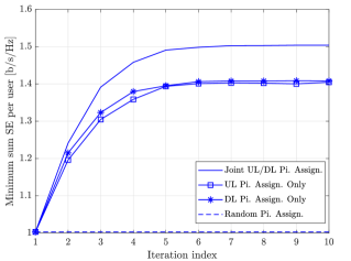
Figs. 2 and 3 display the convergence of proposed pilot assignments for a network with users and users per cell, respectively. The convergence is obtained after less than iterations for all the considered scenarios. When each BS serves users, the sum SE per user converges to about b/s/Hz when utilizing either the uplink or downlink SE as the utility metric to assign the pilot signals. However, relying on the downlink SE to assign the pilot signals yields better the sum SE per user than utilizing the uplink SE when increasing the number of users per cell to users.
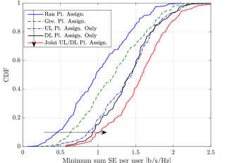
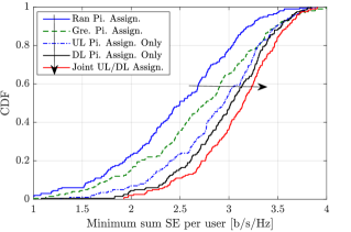
Fig. 4 shows the cumulative distribution function (CDF) of the minimum weighted SE per user for a network where each cell has users. The greedy pilot gives SE better than the random assignment. While assigning the pilot signals based on either the uplink or downlink SE gives almost equivalent performance, but it provides better performance than the random pilot assignment by . Meanwhile, the improvement of joint pilot assignment is up to in weighted minimum sum SE per user compared with the second best and it approves the locality of Algorithm 1. Finally, Fig. 5 manifests the benefits of data power control based on the proposed pilot assignment over the other benchmarks. We observe that the greedy pilot assignment only outperforms the random pilot assignment . Meanwhile, an improvement up to better weighted sum SE per user than random pilot assignment is obtained. In addition, the data power control improves the sum SE per user up to about compared with the fixed data power allocation.
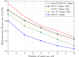
Fig. 6 plots the minimum sum SE per user versus the number of users per cell. Specifically, the minimum sum SE per user decreases when there are more users in the coverage area that generate more mutual interference. For instance, The joint pilot assignment reduce the minimum sum SE per user as the number of user per cell increases from to users. We also observe the benefits of combining the joint pilot assignment and data power control that results in a superior SE improvement up to compared with the random assignment.
V Conclusion
This paper has formulated and solved a max-min sum SE per user optimization problem considering both the pilot assignment and data power control for cellular Massive MIMO systems with correlated Rayleigh channels. We observed significant improvements of pilot assignment to the minimum sum SE per user compared with the other related works. Interestingly, only deploying the uplink or downlink SE as side information to assign pilot still yields good sum SE to weak users if the max-min fairness optimization is considered.
References
- [1] T. L. Marzetta, E. G. Larsson, H. Yang, and H. Q. Ngo, Fundamentals of Massive MIMO. Cambridge University Press, 2016.
- [2] T. A. Le, T. V. Chien, M. R. Nakhai, and T. Le-Ngoc, “Pareto-optimal pilot design for cellular Massive MIMO systems,” IEEE Trans. Veh. Technol., vol. 69, no. 11, pp. 13 206–13 215, 2020.
- [3] T. V. Chien, E. Björnson, and E. G. Larsson, “Joint pilot design and uplink power allocation in multi-cell Massive MIMO systems,” IEEE Trans. Wireless Commun., vol. 17, no. 3, pp. 2000 – 2015, 2018.
- [4] E. Björnson, J. Hoydis, and L. Sanguinetti, “Massive MIMO networks: Spectral, energy, and hardware efficiency,” Foundations and Trends in Signal Processing, vol. 11, no. 3-4, pp. 154 – 655, 2017.
- [5] S. Jin, M. Li, Y. Huang, Y. Du, and X. Gao, “Pilot scheduling schemes for multi-cell massive multiple-input-multiple-output transmission,” IET Commu., vol. 9, no. 5, pp. 689–700, 2015.
- [6] J. C. Marinello Filho, C. M. Panazio, and T. Abrão, “Joint uplink and downlink optimization of pilot assignment for massive mimo with power control,” Trans. Emerging Telecommun. Techno., vol. 28, no. 12, p. e3250, 2017.
- [7] X. Gao, O. Edfors, F. Rusek, and F. Tufvesson, “Massive MIMO performance evaluation based on measured propagation data,” IEEE Trans. Wireless Commun., vol. 14, no. 7, pp. 3899–3911, 2015.
- [8] L. You, X. Gao, X. G. Xia, N. Ma, and Y. Peng, “Pilot reuse for Massive MIMO transmission over spatially correlated Rayleigh fading channels,” IEEE Trans. Wireless Commun., vol. 14, no. 6, pp. 3352–3366, 2015.
- [9] X. Zhu, Z. Wang, L. Dai, and C. Qian, “Smart pilot assignment for Massive MIMO,” IEEE Commun. Lett., vol. 19, no. 9, pp. 1644 – 1647, 2015.
- [10] S. Boyd and L. Vandenberghe, Convex Optimization. Cambridge University Press, 2004.
- [11] A. Krishnamoorthy and D. Menon, “Matrix inversion using Cholesky decomposition,” in Proc. IEEE SPA, 2013.
- [12] H. Boche and M. Schubert, “A general duality theory for uplink and downlink beamforming,” in Proc. IEEE VTC-Fall, 2002, pp. 87–91.