CityNet: A Multi-city Multi-modal Dataset for Smart City Applications

Abstract

Data-driven approaches have been applied to many problems in urban computing. However, in the research community, such approaches are commonly studied under data from limited sources, and are thus unable to characterize the complexity of urban data coming from multiple entities and the correlations among them. Consequently, an inclusive and multifaceted dataset is necessary to facilitate more extensive studies on urban computing. In this paper, we present CityNet, a multi-modal urban dataset containing data from 7 cities, each of which coming from 3 data sources. We first present the generation process of CityNet as well as its basic properties. In addition, to facilitate the use of CityNet, we carry out extensive machine learning experiments, including spatio-temporal predictions, transfer learning, and reinforcement learning. The experimental results not only provide benchmarks for a wide range of tasks and methods, but also uncover internal correlations among cities and tasks within CityNet that, with adequate leverage, can improve performances on various tasks. With the benchmarking results and the correlations uncovered, we believe that CityNet can contribute to the field of urban computing by supporting research on many advanced topics.

1 Introduction

We have witnessed remarkable progress in advancing machine learning techniques (e.g., deep learning [23, 9], transfer learning [15, 19], and reinforcement learning [17, 6]) for various smart city applications [24] in recent years, such as predicting traffic speeds and flows, managing ride-hailing fleets, forecasting urban environments, etc. However, due to the absence of a desirable open-source dataset, most research works in urban computing investigate individual tasks using datasets from limited sources. In fact, existing approaches can be further improved to deliver more intelligent decisions by leveraging data from multiple sources. For example, while most research works on taxi fleet management use taxi data only, in practice, such a task can benefit from additional data sources, including real-time traffic speeds, weather conditions, POI distributions, demands and supplies of other transports, etc. All these urban data are closely related to the taxi market from different aspects. However, existing open datasets, such as PeMS [1], METR [4] and NYC Cabs [2] focus on individual aspects of urban dynamics, e.g., traffic speeds or taxis. Furthermore, limited effort had been spent on unifying the spatio-temporal ranges of existing datasets for joint usage. For example, although TaxiBJ [23], tdrive [21] and Q-traffic [10] all describe Beijing taxi, they are different in temporal ranges and thus cannot be jointly utilized. Hence, an inclusive and spatio-temporally aligned dataset is in urgent demand in urban computing to tackle above problems, so as to facilitate more accurate algorithms and more insightful analyses.

In summary, there are two challenges that hamper building and utilizing such a dataset. First, individual urban datasets from various maintainers differ from each other in spatio-temporal ranges, granularity, attributes, etc. This leads to difficulty in integrating them into unified formats under aligned ranges and granularities for research purposes. Second, in addition to the dataset construction, the correlations among sub-datasets must be uncovered so as to enhance performances by identifying, sharing, and transferring related knowledge.

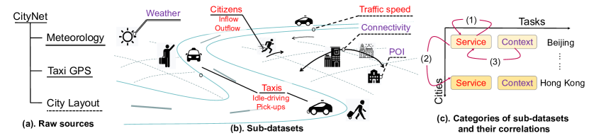
Figure 1: Architecture of CityNet. Left: Three raw data sources of CityNet. Middle: Illustration of all 8 sub-datasets, whose sources are distinguished by underlines shown in Fig. 1(a), and categories are distinguished by colors shown in Fig. 1(c). Right: Decomposition of the data dimensions into cities and tasks. Directed curves indicate correlations to be discovered in this paper.

In this paper, we present CityNet, a dataset with data from multiple cities and sources for smart city applications. Inspired by [16], we call CityNet multi-city multi-modal to describe the wide range of cities and sources from which it is derived. Compared to existing datasets, CityNet has the following features:

• Inclusiveness: As shown in Fig. 1(a), CityNet consists of 3 types of raw data (city layout, taxi, meteorology) collected from 7 cities. Besides, we process the raw data into multiple sub-datasets (Fig. 1(b)) to measure various aspects of urban phenomena. For example, we transform raw taxi data into region-based measurements (taxi flows, pickups, and idle driving time) that show the status of the transportation market and citizen activities.

• Spatio-temporal Alignment: To facilitate studies among cities and tasks, we use unified spatio-temporal configuration, including geographical coordinates, temporal frames, and sampling intervals to process all sub-datasets originating from the same city.

• Interrelatedness: We categorize sub-datasets into service and context data, as shown in Fig. 1(b) and (c), to demonstrate the status of urban service providers (e.g. taxi companies) and the urban environment (e.g. weather) respectively. As depicted in Fig. 1(c), we verify the correlations between sub-datasets, including the relationship (1) among services, (2) between cities and (3) between contexts and services.

Leveraging the above features of CityNet, we conduct a series of experiments to benchmark various popular machine learning tasks, including spatio-temporal prediction, transfer learning and reinforcement learning. The empirical studies reveal that utilizing such a multi-modal dataset leads to performance improvements, and also point to the current challenges and future opportunities.

The contributions of this paper are summarized as follows:

• To the best of our knowledge, CityNet is the first multi-city multi-modal urban dataset to assemble and align sub-datasets from different tasks and cities. It is open to the research community and can facilitate in-depth investigations on urban phenomenons from various disciplines.

• Extensive analysis and experiments on CityNet provide new insights for researchers. Upon CityNet, we present diverse benchmarking results so as to motivate further studies in areas like spatio-temporal predictions, transfer learning, reinforcement learning, and federated learning in urban computing. Specifically, we use various tools to reveal and quantify the correlations among different modalities and cities. We further demonstrate that appropriately utilizing the mutual knowledge among correlated sub-datasets can significantly improve the performance of various machine learning tasks.

CityNet has been open-sourced and is currently accessible at https://github.com/citynet-at-git/Citynet-phase1. Besides, to empower the most advanced research in urban computing, we also plan to share all resources related with this paper on TACC, a high-performance computing platform currently in the initial stages of opening to the public. Please refer to Appendix A.7 for details.

2 Architecture of CityNet

In this section, we introduce the generation of CityNet, including the raw datasets, discretization, generation of individual datasets and data integration across individual datasets.

2.1 Raw Data Collection

Taxi GPS points

Taxi trajectories reflect rich information on citizen activities and the status of the transportation network. We collect taxi GPS point records $\mathcal{G}_{c}$ in each city $c$, which consist of trajectories of taxis $\mathcal{G}_{c}=\{tr_{a}\}_{a\in\mathcal{A}_{c}}$, where $\mathcal{A}_{c}$ is the set of taxis in city $c$. Each trajectory $tr_{a}$ is a sequence of tuples $tr_{a}=\left[\left(pos_{k},t_{k},occ_{k}\right)\right]_{k=1}^{|tr_{a}|}$, where $pos_{k}$ denotes the position (i.e. longitude and latitude) of the taxi at time $t_{k}$, and $occ_{k}$ denotes whether the taxi is occupied at time $t_{k}$.

City Layout data

We collect POI (points-of-interest), road network and traffic speed data to describe the overall layout of the city. POI data ($\mathbf{x}^{poi}$) describe the functions served by each region. A POI is defined as $poi=(pos_{poi},cat_{poi})$, where $pos_{poi}$ denotes the position (longitude and latitude) of the POI, and $cat_{poi}$ denotes the category (e.g., catering, shopping) of the POI. We denote the set of all POIs in city $c$ as $POI_{c}$. The road network and traffic speed data ($\mathbf{x}^{speed}$) describe the real-time status of the transportation system. A road segment is defined by its two endpoints as $seg=(pos_{0},pos_{1})$. Each segment is associated with its historical real-time traffic speeds $sp_{seg}=[(t_{k},speed_{k})]_{k=1}^{|sp_{seg}|}$, where $speed_{k}$ denotes the speed of $seg$ at time $t_{k}$.

Meteorology data

We collect weather data recorded at the airport of each city from rp5 every hour. We process the weather data of each city into a matrix $\mathbf{x}_{c}^{mtr}\in\mathbb{R}^{T_{c}/2\times 49}$, where each 49-dimensional vector contains information about temperature, air pressure, humidity, weather phenomena (e.g., rain, fog), etc. We describe the detailed schema of the weather data in the Appendix A.3.

In total, we collect data for 7 cities: Beijing, Shanghai, Shenzhen, Chongqing, Xi’an, Chengdu and Hong Kong. We provide data properties, including data range, size, and availability in Table 5, and summarize notations used in this paper in Table 7 in the Appendix.

2.2 Raw Data Discretization

Discretization is the first pre-processing step that transforms raw datasets from continuous spatio-temporal ranges to discrete space with fixed sampling intervals. This procedure enables building indicators via aggregating discretized measurements from the same interval to quantify various phenomena in cities. The formulations of the discretization in both spatial and temporal dimensions are defined as follows:

Definition 1 (Region).

Each city $c$ is split into $W_{c}\times H_{c}$ square grids, each with size 1km$\times$1km. Each grid in a city is referred to as a region, denoted as $r$. We denote the set of all regions in city $c$ as $\mathcal{R}_{c}$, and use $r_{c}(i,j)$ to denote the region in city $c$ with coordinate $(i,j)$.

Definition 2 (Timestamps).

We define the set of available time stamps of city $c$ as $\mathcal{T}_{c}=[\tau_{c}-T_{c}+1,...\tau_{c}]$, where $\tau_{c}$ denotes the last timestamp, and $T_{c}$ is the number of available time stamps of city $c$. By default, we choose each time stamp to be a period of 30 minutes.

Definition 3 (Spatio-temporal Tensors).

We denote a spatio-temporal tensor for city $c$ (e.g. taxi flow values) as $\mathbf{x}_{c}\in\mathbb{R}^{T_{c}\times W_{c}\times H_{c}}$, and use $\mathbf{x}_{c}(\tau,i,j)$ and $\mathbf{x}_{c}(\tau)$ to denote the value at region $r_{c}(i,j)$ and the values for all regions in city $c$ at timestamp $\tau$, respectively.

2.3 Processing Individual Sub-datasets

Taxi Flow Dataset

Region-wise human flows are important to traffic management and public safety. Given taxi GPS points $\mathcal{G}_{c}$, we extract inflow and outflow spatio-temporal tensors $\mathbf{x}^{in}_{c},\mathbf{x}^{out}_{c}\in\mathbb{R}^{T_{c}\times W_{c}\times H_{c}}$ as the number of taxis going into and out of each region within a timestamp [22]:

$$\mathbf{x}^{in}_{c}(\tau,i,j)=\sum_{tr\in\mathcal{G}_{c}}\sum_{(pos_{k},t_{k},occ_{k})\in tr}\mathbb{I}\left(t_{k}\in\tau\land pos_{k}\in r_{c}(i,j)\land pos_{k-1}\notin r_{c}(i,j)\right),$$ (1)

$$\mathbf{x}^{out}_{c}(\tau,i,j)=\sum_{tr\in\mathcal{G}_{c}}\sum_{(pos_{k},t_{k},occ_{k})\in tr}\mathbb{I}\left(t_{k+1}\in\tau\land pos_{k}\in r_{c}(i,j)\land pos_{k+1}\notin r_{c}(i,j)\right),$$

where $\mathbb{I}(X)$ is the indicator function. $\mathbb{I}(X)=1$ iff $X$ is true.

Taxi Pickup and Idle Driving Dataset

Demand and supply data of taxis are also important to allocating transportation resources efficiently. Given taxi GPS points $\mathcal{G}_{c}$, we derive the pickup and idle driving spatio-temporal tensors $\mathbf{x}_{c}^{pickup},\mathbf{x}_{c}^{idle}$ to approximate the demands and supplies of taxis.

$$\mathbf{x}_{c}^{pickup}(\tau,i,j)=\sum_{tr\in\mathcal{G}_{c}}\sum_{(pos_{k},t_{k},occ_{k})\in tr}\mathbb{I}(t_{k}\in\tau\land occ_{k}=1\land occ_{k-1}=0),$$ (2)

$$\mathbf{x}_{c}^{idle}(\tau,i,j)=\frac{1}{|\tau|}\sum_{tr\in\mathcal{G}_{c}}\sum_{(pos_{k},t_{k},occ_{k})\in tr}\mathbb{I}(t_{k}\in\tau\land occ_{k}=0)(t_{k+1}-t_{k}),$$ (3)

where $|\tau|$ denotes the length of a timestamp. Eqn. 2 computes the number of pickups of all taxis at $r_{c}(i,j)$ at timestamp $\tau$, which serves as a lower bound for taxi demands. Meanwhile, Eqn. 3 computes the total fraction of time in timestamp $\tau$ where taxis are running in idle.

POI Dataset

For city $c$, we obtain POI data $POI_{c}=\{(pos_{poi},cat_{poi})\}$ using AMap API . Each POI category is given an id from 0 to 13. We build POI tensors $\mathbf{x}^{poi}_{c}\in\mathbb{R}^{W_{c}\times H_{c}\times 14}$ as follows:

$$\mathbf{x}^{poi}_{c}(i,j,cat)=\sum_{(pos_{poi},cat_{poi})\in POI_{c}}\mathbb{I}(cat_{poi}=cat\land pos_{poi}\in r_{c}(i,j)).$$ (4)

$\mathbf{x}_{c}^{poi}(i,j,cat)$ is the number of POIs with category $cat$ in $r_{c}(i,j)$.

Road Connectivity Dataset

We collect road map information, including highways and motorways from OpenStreetMaps. According to the road maps, we build region-wise adjacency matrices $\mathbf{A}^{conn}_{c}\in\mathbb{R}^{|\mathcal{R}_{c}|\times|\mathcal{R}_{c}|}$ as:

$$\mathbf{A}^{conn}_{c}(r_{0},r_{1})=\sum_{(pos_{0},pos_{1})\in SEG_{c}}\mathbb{I}(pos_{0}\in r_{0}\land pos_{1}\in r_{1}),$$ (5)

where $r_{0},r_{1}\in\mathcal{R}_{c}$. $\mathbf{A}^{conn}_{c}(r_{0},r_{1})$ represents the total number of roads connecting $r_{0}$ and $r_{1}$, and therefore, $\mathbf{A}_{c}^{conn}$ represents region-wise transportation connectivity within city $c$.

Traffic Speed Dataset

The real-time speed data are processed into $\mathbf{x}^{speed}_{c}\in\mathbb{R}^{T_{c}\times|SEG_{c}|}$:

$$\mathbf{x}^{speed}_{c}(\tau,s)=\sum_{s\in SEG_{c}}\frac{\sum_{(t_{k},speed_{k})\in sp_{s}}\mathbb{I}(t_{k}\in\tau)\cdot speed_{k}}{\sum_{(t_{k},speed_{k})\in sp_{s}}\mathbb{I}(t_{k}\in\tau)}.$$ (6)

It indicates the average traffic speed of the road segment $s$ over timestamp $\tau$.

As shown in Fig. 1(c), we categorize all taxi data (flow, pickup, and idle driving data) and traffic speed data as service data as they represent the states of transport service providers, and the rest as context data. We show statistics of all sub-datasets in Table 6 in the Appendix.

2.4 Data integration

Service data and context data are usually integrated to jointly train machine learning models. In CityNet, such a integration operation is simple using the ’JOIN’ operation on the aligned spatial or temporal dimension. Using the taxi demand prediction problem as an example, we can represent the integration of taxi pick-up data, POI data and meteorology data with the following relational algebra formula: $\Pi_{*}(\mathbf{x}_{c}^{poi}\Join_{(i,j)}\mathbf{x}_{c}^{pickup}\Join_{\tau}\mathbf{x}_{c}^{mtr})$, which represents joining pick-up data with POI data on the spatial dimension and joining pick-up data with meteorology data on the temporal dimension.

3 Data Mining and Analysis

In addition to data gathering and processing, we should also uncover and quantify the correlations between sub-datasets in CityNet to provide insights on how to utilize the multi-modal data. In this section, we use data mining tools to explore the correlations between service data and context data.

	Inflow	Outflow	Pickup	Idle-time	Inflow	Outflow	Pickup	Idle-time	Inflow	Outflow	Pickup	Idle-time
	Beijing				Shanghai				Shenzhen
ARI	0.554	0.554	0.635	0.544	0.445	0.445	0.474	0.382	0.191	0.191	0.219	0.227
AMI	0.308	0.308	0.418	0.318	0.268	0.268	0.356	0.240	0.132	0.132	0.192	0.182
	Chongqing				Chengdu				Xi’an
ARI	0.471	0.471	0.624	0.541	0.197	0.196	0.167	N/A	0.155	0.155	0.042	N/A
AMI	0.261	0.261	0.404	0.350	0.213	0.213	0.226	N/A	0.164	0.164	0.05	N/A

Table 1: ARI and AMI measurements between clustering assignments based on POI and those based on taxi data. Both measurements range from $[-1,1]$. Larger values indicate higher coincidence.

3.1 Correlation between POI and Taxi Data

Intuitively, taxi service data should be closely related to POIs. For example, the outflow of residential areas should grow significantly in morning peak hours, while taxi pickups should be frequent in business areas during evening rush hours. To confirm this, we cluster regions in city $c$ to $k=3$ disjoint clusters as: $\mathbb{C}_{c,poi}:\mathcal{R}_{c}=\mathcal{R}_{c,1}\cup\mathcal{R}_{c,2}\cup\cdots\cup\mathcal{R}_{c,k}$, according to their POI vectors ($\mathbf{x}_{c}^{poi}$) using the k-means algorithm. Similarly, we also cluster regions using the average daily pattern of taxi service data to obtain $\mathbb{C}_{c,in}$, $\mathbb{C}_{c,out}$, $\mathbb{C}_{c,pickup}$, $\mathbb{C}_{c,idle}$. We use the Adjusted Rand Index (ARI) and the Adjusted Mutual Information (AMI) to measure the similarity between cluster assignments based on POIs ($\mathbb{C}_{c,poi}$) and those based on taxi service data ($\mathbb{C}_{c,in}$, etc). The results are shown in Table 1, where both ARI and AMI show positive correlations between both cluster assignments, which confirms the relationship between the POI data and taxi service data.

Further more, we plot the average regional daily patterns of taxi service data from each POI-based cluster in Beijing, Chengdu, and Xi’an in Fig. 2 in the Appendix. On one hand, in Fig. 2(a), taxi patterns in Beijing are cohesive within each POI-based cluster and separable across clusters. On the other hand, in Fig. 2(b), clusters with higher values significantly overlap in Xi’an and Chengdu, which are cities with relatively low ARI and AMI in Table 1. This may be caused by the limited number of regions in these cities. However, we can still identify two separable clusters in Fig. 2(b).

According to the results, we conclude that regions with similar POI distributions also share similar taxi service patterns.

3.2 Correlation between Meteorology and Traffic Speed Data

	Xi’an	Chengdu
Rain	-2.06∗∗	-0.64∗
Fog	-0.78∗∗	-0.79∗∗

Table 2: Regression coefficients between weather phenomena and traffic speed in Chengdu and Xi’an. ${}^{*},^{**}$ indicate 5% and 1% significance under a double-sided t-test, respectively.

It is also intuitive that there exists correlations between weather and traffic speed. For example, when confronted with rain or fog, drivers tend to drive with caution and thus slow down. Therefore, we perform experimental studies to verify the correlations.

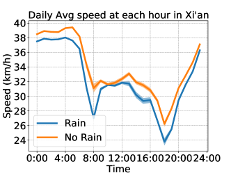
(a) Rain

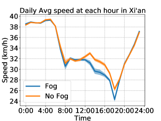
(b) Fog

Figure 3: Daily average speed in Xi’an, with and without rain or fog. Shades represent half of the standard deviation.

We perform both quantitative and qualitative studies. For quantitative studies, we perform least squares regression on the average speed for each timestamp $\tau$, i.e. $\mathrm{MEAN}_{s}\left(\mathbf{x}_{c}^{speed}\left(\tau,s\right)\right)$ with the weather phenomena $\mathbf{x}^{mtr}_{c}(\tau)$, and show the coefficients in Table 2. It can be shown that both rain and fog have negative effects on the average traffic speed. We also plot the daily average speeds in Xi’an, with and without rain or fog in Fig. 3 in the Appendix. We observe consistently higher average speeds when there was no rain, and higher average speeds during day time when there was no fog.

City	Task	Non Deep Learning		Euclidean Deep Learning				Graph Learning
RMSE/MAE		ST-HA	ST-LR	ST-CNN	MT-CNN	ST-LSTM	MT-LSTM	ST-GCN	MT-GCN	ST-GAT	MT-GAT
Beijing	Inflow	7.90/2.97	6.07/2.59	5.60/2.35	5.45/2.39	5.67/2.31	5.48/2.40	5.48/2.27	5.34/2.19	5.59/2.43	5.36/2.20
	Outflow	7.90/2.97	6.07/2.59	5.60/2.35	5.45/2.39	5.67/2.31	5.48/2.40	5.48/2.27	5.33/2.19	5.59/2.43	5.36/2.20
	Pickup	2.51/0.90	2.37/0.89	2.19/0.79	2.15/0.82	2.24/0.82	2.14/0.80	2.23/0.82	2.14/0.80	2.15/0.80	2.14/0.79
	Idle	0.73/0.31	0.61/0.25	0.57/0.24	0.54/0.25	0.60/0.25	0.52/0.22	0.55/0.24	0.51/0.23	0.55/0.24	0.50/0.22
Shanghai	Inflow	19.41/7.93	11.72/5.93	8.29/4.36	8.41/4.51	8.60/4.57	8.67/4.60	10.40/5.26	9.77/5.05	10.05/5.11	9.64/4.99
	Outflow	19.40/7.94	11.76/5.94	8.42/4.42	8.26/4.43	8.64/4.53	8.52/4.51	10.07/5.14	9.49/4.90	10.10/5.13	9.38/4.89
	Pickup	2.24/0.88	1.94/0.84	1.66/0.75	1.64/0.75	1.66/0.74	1.61/0.73	1.78/0.79	1.72/0.80	1.75/0.77	1.71/0.76
	Idle	1.23/0.54	0.89/0.41	0.86/0.44	0.75/0.41	0.85/0.41	0.73/0.36	0.86/0.42	0.79/0.38	0.81/0.40	0.78/0.38
Shenzhen	Inflow	43.79/18.97	24.06/12.23	17.62/9.41	18.28/9.75	17.94/9.57	17.75/9.65	22.18/11.61	20.84/10.91	22.35/11.46	20.52/10.87
	Outflow	43.85/18.97	24.08/12.23	18.08/9.54	18.45/9.53	17.70/9.54	17.80/9.64	22.08/11.33	20.82/10.81	21.99/11.28	20.59/10.82
	Pickup	6.78/2.48	4.91/2.09	4.29/1.83	4.24/1.76	4.00/1.75	3.99/1.76	4.39/2.02	4.24/1.86	4.50/1.92	4.21/1.84
	Idle	4.25/1.59	2.51/1.09	2.29/0.98	2.16/1.00	1.88/0.88	1.90/0.93	2.33/1.05	2.17/0.97	2.29/1.01	2.18/0.98
Chongqing	Inflow	37.40/14.97	21.19/9.91	12.65/6.48	12.67/6.52	14.39/7.29	13.84/7.08	18.54/6.59	17.12/8.46	16.53/8.49	15.98/7.93
	Outflow	37.36/14.87	21.23/9.85	12.90/6.60	12.99/6.60	14.30/7.10	13.68/6.95	18.75/8.87	16.91/8.29	18.12/9.12	15.94/7.93
	Pickup	7.64/3.03	6.34/2.69	5.25/2.24	5.15/2.10	5.21/2.18	5.02/2.10	5.77/2.45	5.49/2.33	5.72/2.45	5.34/2.28
	Idle	3.81/1.48	2.21/0.96	1.53/0.74	1.57/0.76	1.58/0.73	1.57/0.75	1.99/0.87	1.90/0.84	1.97/0.86	1.80/0.83
Xi’an	Inflow	87.00/55.28	43.69/29.72	27.79/19.20	25.77/17.85	28.13/19.39	26.33/17.94	34.77/23.86	31.70/21.77	31.62/21.67	30.67/21.59
	Outflow	86.66/55.29	43.58/29.59	27.59/18.97	25.32/17.55	27.90/18.19	25.92/17.69	35.24/24.15	31.04/21.49	29.88/22.18	28.96/20.12
	Pickup	16.85/10.84	11.22/7.66	7.77/5.39	7.54/5.16	7.88/5.38	7.71/5.27	9.50/6.50	9.11/6.26	8.22/5.88	8.05/5.26
Chengdu	Inflow	117.5/71.1	58.92/37.72	31.22/21.09	30.02/20.40	34.50/23.57	32.78/22.42	45.10/29.49	41.27/27.62	40.02/27.27	38.47/25.84
	Outflow	116.9/71.5	58.98/37.88	31.91/21.46	29.74/20.20	33.55/22.86	32.77/22.22	43.66/28.47	40.39/27.10	35.59/24.72	35.20/24.58
	Pickup	28.27/15.66	17.32/10.54	11.02/7.13	10.55/6.78	11.39/7.21	11.15/7.15	13.64/8.55	13.58/8.76	12.30/7.62	11.24/7.38

Table 3: Results for taxi prediction of all models and all tasks under 6 cities. ST-* and MT-* stands for single-task and multi-task models respectively. The lowest RMSE/MAE in each task are bolded.

4 Machine Learning Applications

In this section, we present experimental results of machine learning tasks that are supported by CityNet, including spatio-temporal predictions (Section 4.1.1 and Appendix A.5.1), transfer learning (Section 4.2), and reinforcement learning (Appendix A.5.2) to benchmark individual tasks. Also, the benchmark results uncover the transferrability of knowledge across tasks and cities in CityNet.

4.1 Spatio-temporal Predictions

Spatio-temporal predictions are common and important tasks in smart city. Given the data in CityNet, we provide benchmarks for two typical spatio-temporal prediction tasks, including the taxi service prediction tasks in Section 4.1.1, and the traffic speed prediction task in Appendix A.5.1.

4.1.1 Taxi Service Prediction

We investigate the taxi service prediction task [22, 3], including flow and demand-supply prediction.

Problem Formulation

We formulate the taxi service prediction problem as learning a single-step prediction function $f_{c}$ that achieves the lowest prediction error over future timestamps:

$$\tilde{\mathbf{x}}_{c}^{*}(\tau) =\tilde{f}_{c}\left(\left[\mathbf{x}_{c}^{*}(\tau-L),...,\mathbf{x}_{c}^{*}(\tau-1)\right]\right),$$ (7)

$$f_{c} =\arg\min_{\tilde{f}_{c}}\sum_{\tau\in\mathcal{T}_{c}}error\left(\tilde{\mathbf{x}}_{c}^{*}\left(\tau\right),\mathbf{x}_{c}^{*}\left(\tau\right)\right).$$

$$* =in,out,pickup,idle,joint,$$

where $\mathbf{x}_{c}^{*}$ stands for the spatio-temporal tensor to predict, and $error$ denotes some error function, such as RMSE or MAE. We introduce two settings, the single-task and multi-task settings, where $\mathbf{x}_{c}^{*}$ denotes individual spatio-temporal tensors (e.g. in/outflow) for the single-task setting, and the stacked spatio-temporal tensors $\mathbf{x}_{c}^{joint}=\mathrm{STACK}\left(\left[\mathbf{x}_{c}^{in},\mathbf{x}_{c}^{out},\mathbf{x}_{c}^{pickup},\mathbf{x}_{c}^{idle}\right]\right)$ for the multi-task setting. In other words, we achieve multi-task learning for multiple taxi service predictions through direct weight sharing. We set the input as $L=5$ closest temporal observations (i.e., 2.5 hours).

Methods

We study the following methods for taxi prediction.

• HA (History Average): Mean of historical values of the data.

• LR (Linear Regression): Ridge regression on historical values with a regularization of 0.01.

• CNN (Convolutional Neural Network): We implement our CNN based on STResNet [22]. We use 6 residual blocks with 64 $3\times 3$ filters. Batch normalization (BN) is used.

• LSTM: We implement our LSTM based on ST-net [19], which first uses convolutions to model spatial relations and uses LSTM to capture temporal dependencies. We use 3 residual blocks with BN for convolutions, and use a single-layer LSTM with 256 hidden units.

• GCN (Graph Convolutional Network) [5] and GAT (Graph Attention Network) [14]: We apply GCN and GAT with input features being historical values (single-task) or stacked historical values of all tasks (multi-task) of input data. For graph convolution, we take the adjacency matrix as $\mathbf{A}=\left(\mathbf{A}_{c}^{conn}+\mathbf{A}_{c}^{poi}+\mathbf{A}_{c}^{neigh}\right)/3$ following [3], and use the normalized adjacency matrix $\hat{\mathbf{A}}=\mathbf{D}^{-1/2}\mathbf{A}\mathbf{D}^{-1/2}$ for GCN.

Among them, HA, LR are traditional time series forecasting models, CNN, LSTM are deep learning models on Euclidean structures (grids), while GCN, GAT are graph deep learning models utilizing additional region-wise connections (e.g. POI and road connectivity).

Experimental Settings

We split the earliest 70% data for training, the middle 15% for validation, and the latest 15% for testing. All data are normalized to $[0,1]$ by min-max normalization and will be recovered for evaluation. We use RMSE and MAE as metrics [20].

Table 3 shows the overall performances under both the single-task (ST-*) setting and the multi-task (MT-*) setting for all investigated models. We make the following observations:

• Deep Learning or Not: Given sufficient data (e.g. 10 days, 1-2 months), deep learning models including CNN, LSTM, GCN, and GAT outperform time-series forecasting methods like HA and LR. This illustrates the power of deep learning in spatio-temporal predictions and the advantage of leveraging correlations in both Euclidean and non-Euclidean spaces.

• Multi-task or Not: Among all 22 tasks, multi-task models achieve the lowest RMSE in 15 (68.2%) tasks, and the lowest MAE in 15 (68.2%) tasks. For each model, MT-* outperforms ST-* in 80 (90.9%) cases in terms of RMSE and 66 (75%) cases in terms of MAE. We conclude that taxi service predictions can be improved through a simple multi-task method, weight sharing, which verifies the connections among heterogeneous taxi service data and paves way for future research in multi-task spatio-temporal predictions.

• Graph Models or Not: Among all the prediction tasks, CNN-based models (CNN, LSTM) achieve the best performances in most cases, while GNN-based models (GCN, GAT) work well in Beijing only, which has the largest map size with the most complex intra-city relations. We conclude that in cities with large map sizes, incorporating graphs to model region-wise connections will improve prediction accuracy, while in cities with small map sizes, incorporating graphs will hurt performance. One possible reason is that graphs built on a limited number of regions tend to be dense, as shown in Table 6, which causes over-smoothing [7].

Target City	Task	Full Data (Lower bound)		3-day Data (Upper bound)		Fine-tuning/Source City			RegionTrans/Source City
		LR	LSTM	LR	LSTM	Beijing	Shanghai	Xi’an	Beijing	Shanghai	Xi’an
Shenzhen	Inflow	24.06/12.23	17.94/9.57	24.07/12.27	22.63/12.83	19.78/10.58	20.90/11.09	N/A	19.67/10.40	20.59/10.93	N/A
	Outflow	24.08/12.23	17.80/9.64	24.09/12.27	22.75/12.87	19.82/10.58	20.95/11.09	N/A	19.62/10.49	20.70/10.95	N/A
	Pickup	4.91/2.09	3.99/1.76	4.92/2.09	4.52/2.07	4.25/1.86	4.37/1.92	N/A	4.21/1.82	4.31/1.89	N/A
	Idle	2.51/1.09	1.90/0.94	2.51/1.09	2.39/1.17	2.12/0.97	2.16/1.10	N/A	2.12/0.97	2.13/1.00	N/A
Chongqing	Inflow	21.19/9.91	13.84/7.08	21.20/9.95	18.45/9.81	16.10/7.98	16.74/8.23	N/A	15.87/7.90	16.59/8.15	N/A
	Outflow	21.24/9.85	13.68/6.95	21.24/9.86	18.22/9.69	15.85/7.83	16.61/8.13	N/A	15.72/7.83	16.46/8.08	N/A
	Pickup	6.34/2.69	5.02/2.10	6.34/2.69	5.64/2.52	5.42/2.23	5.45/2.30	N/A	5.37/2.20	5.42/2.30	N/A
	Idle	2.21/0.96	1.57/0.75	2.21/0.96	2.03/0.98	1.75/0.81	1.80/0.83	N/A	1.77/0.82	1.77/0.81	N/A
Chengdu	Inflow	58.92/37.72	32.79/22.42	59.29/38.45	48.39/33.12	43.49/28.88	46.30/30.08	45.24/29.69	43.43/28.60	45.74/29.92	44.43/29.51
	Outflow	58.98/37.88	33.55/22.86	59.37/38.61	47.77/32.69	43.12/28.44	46.06/30.12	44.66/29.35	42.73/28.66	45.59/29.86	43.69/29.17
	Pickup	17.32/10.54	11.15/7.15	17.40/10.69	15.21/10.08	13.78/8.79	14.39/9.12	14.07/9.01	13.51/8.48	14.21/9.03	13.89/9.06

Table 4: Results for inter-city transfer learning from source cities (Beijing, Shanghai, Xi’an) to target cities (Shenzhen, Chongqing, Chengdu). The lowest RMSE/MAE using limited target data are in bold. Results under full and 3-day data are lower and upper bounds of errors of corresponding tasks.

4.2 Inter-city Transfer Learning

As shown in Table 3, deep learning models generate accurate predictions when empowered with abundant data. However, the level of digitization varies significantly among cities, and it is likely that many cities cannot build accurate deep prediction models due to a lack of data. One solution to the problem is transfer learning [12], which transfers knowledge from a source domain with abundant data to a target domain without much data, and in our case, from one city to another. Therefore, we carry out transfer learning experiments on CityNet to show that connections among cities can lead to positive knowledge transfer, and to provide benchmarks for future works on urban transfer learning.

We investigate the problem of inter-city transfer learning on taxi service datasets. We formulate the problem as to learn a function $f_{c_{s},c_{t}}$ that achieves the lowest prediction error on the target city $c_{t}$, with the help of data from the source city $c_{s}$:

$$\tilde{\mathbf{x}}_{c_{t}}^{*}(\tau) =\tilde{f}_{c_{s},c_{t}}\left(\left[\mathbf{x}_{c_{t}}^{*}(\tau-L),...,\mathbf{x}_{c_{t}}^{*}(\tau-1)\right],\mathbf{x}_{c_{s}}^{*}\right),$$ (8)

$$f_{c_{s},c_{t}} =\arg\min_{\tilde{f}_{c_{s},c_{t}}}\sum_{\tau\in\mathcal{T}_{c_{t}}}error\left(\tilde{\mathbf{x}}_{c_{t}}^{*}(\tau),\mathbf{x}_{c_{t}}^{*}(\tau)\right).$$

$$* =in,out,pickup,idle,joint,|\mathbf{x}_{c_{t}}^{*}|\ll|\mathbf{x}_{c_{s}}^{*}|.$$

Experimental Settings

We use LSTM, which is similar to ST-net in MetaST [19] as the base model, and adopt the multi-task setting. For cities with large map sizes, we choose Beijing and Shanghai to be source cities; for those with small map sizes, we choose Xi’an to be the source city, and the rest are chosen as target cities. Xi’an is not used as the source city to transfer to Shenzhen and Chongqing due to its much smaller map size. For all target cities, we choose a three-day, Thursday-Friday-Saturday interval for training, and validation and test data remain the same.

Methods

We study the following transfer learning methods:

• Fine-tuning: We train a model on the source city and then tune it on limited target data.

• RegionTrans [15]: RegionTrans computes a matching between source $\mathcal{R}_{c_{s}}$ and target regions $\mathcal{R}_{c_{t}}$ based on time-series (S-match) or auxiliary data (A-match) correlation. The matching is used as a regularizer, such that similar regions share similar features. In our experiments, we use POI vectors to compute the matching, which belongs to A-match.

Results

We show results of inter-city transfer learning in Table 4. We show results trained using full and 3-day target data, which correspond to the lower and upper bound of errors, respectively. We also show results of fine-tuning and RegionTrans. We make the following observations:

• Degradation under Data Scarcity. When only 3-day training data are available, LR, as a non-deep learning model achieves similar performances as using full data, while LSTM suffers from 50% more error (see Chengdu). It indicates that compared to non-deep learning, deep learning models show greater sensitivity to the amount of training data.

• Inter-city Correlations. Compared to using target data only (upper bound), transfer learning achieves error reductions in all source-target pairs, the largest of which is about 15% (see Shenzhen and Chongqing). The results indicate that there exist sufficient cross-city correlations in CityNet, such that knowledge learned for one city can be beneficial to another.

• Impact of Context Data. Using POI data for region matching, RegionTrans achieves lower error than fine-tuning in most cases, which verifies the connection between context and service data, and underscores the importance of multi-modal data in CityNet.

• Domain Selection. We consistently achieve the best results when Beijing is used as the source city, regardless of algorithms and the target city. One probable reason is that Beijing contains the most regions, and hence the most complex regional service patterns.

4.3 Discussion

The spatio-temporal prediction experiments on the taxi service data have uncovered the correlation among different tasks for individual sub-datasets in CityNet. Leveraging the mutual knowledge among them, the prediction performances for individual tasks could be improved by simple multi-task learning strategies like weight sharing. Also, via transfer learning, the cold start problem in data-scarce cities could be alleviated by choosing a highly-related source domain and transfer the abundant knowledge learned from it. This is supported by the cross-city correlations in CityNet.

To summarize, both the multi-task spatio-temporal prediction and the inter-city transfer learning demonstrate the correlations among individual datasets in CityNet from different tasks and cities. Thus, the inclusiveness and interrelatedness of CityNet are important features to facilitate the research of various urban phenomena with new problem settings and new techniques.

5 Conclusion and Opportunities

We present a multi-city, multi-modal dataset for smart city named CityNet. To the best of our knowledge, CityNet is the first dataset to incorporate urban data that are spatio-temporally aligned from multiple cities and tasks. In this paper, to illustrate the importance of multi-modal urban data, we show connections between service and context data using data mining tools, and provide extensive experimental results on spatio-temporal predictions, transfer learning, and reinforcement learning to show the connections among tasks and among cities. The results and the uncovered connections endorse the potential of CityNet to serve as versatile benchmarks on various research topics, including but not exclusive to:

• Transfer learning: In urban computing, knowledge required for different tasks, cities, or time periods is likely to be correlated. Leveraging the transferable knowledge across these domains, data scarcity problems in newly-built or under-developed cities can be alleviated. Containing multi-city, multi-task data, CityNet is an ideal testbed for researchers to develop and evaluate various transfer learning algorithms, including meta-learning [19], AutoML [8], and also transfer learning on homogeneous or heterogeneous spatio-temporal graphs.

• Federated learning: Urban data are generated by various human activities and warehoused by different stakeholders, including organizations, companies, and the government. Due to data privacy regulations or the protection of commercial interests, collaborations between them should be privacy-preserving. Federated learning (FL) [18] would become an effective solution enabling such privacy-preserving multi-party collaboration. As CityNet contains data from multiple cities and sources, it is appropriate to investigate various FL topics under various settings using CityNet, with each party holding data from one source or one city.

• Explanation and diagnosis: Understanding social effects from data helps city governors make wiser decisions on urban management. Therefore, besides to prediction and planning, we hope that applications providing explicit insight into urban management, including causal inference [11], uncertainty estimations, explainable machine learning can also be carried out on CityNet.

We hope CityNet can serve as triggers that lead to more extensive research efforts into machine learning in smart city. For future work, we notice that CityNet is not yet multi-modal in terms of transports, and thus plan to incorporate even more sources of data into CityNet, including subways and buses.

Checklist

1. For all authors…

   1. Do the main claims made in the abstract and introduction accurately reflect the paper’s contributions and scope? [Yes]

   2. Did you describe the limitations of your work? [Yes]

   3. Did you discuss any potential negative societal impacts of your work? [No] We only publish the discretized and aggregated measurements of our dataset, which will not reveal sensitive information of individual users.

   4. Have you read the ethics review guidelines and ensured that your paper conforms to them? [Yes]

2. If you are including theoretical results…

   1. Did you state the full set of assumptions of all theoretical results? [N/A]

   2. Did you include complete proofs of all theoretical results? [N/A]

3. If you ran experiments (e.g. for benchmarks)…

   1. Did you include the code, data, and instructions needed to reproduce the main experimental results (either in the supplemental material or as a URL)? [Yes]

   2. Did you specify all the training details (e.g., data splits, hyperparameters, how they were chosen)? [Yes]

   3. Did you report error bars (e.g., with respect to the random seed after running experiments multiple times)? [No]

   4. Did you include the total amount of compute and the type of resources used (e.g., type of GPUs, internal cluster, or cloud provider)? [Yes]

4. If you are using existing assets (e.g., code, data, models) or curating/releasing new assets…

   1. If your work uses existing assets, did you cite the creators? [Yes]

   2. Did you mention the license of the assets? [Yes]

   3. Did you include any new assets either in the supplemental material or as a URL? [No]

   4. Did you discuss whether and how consent was obtained from people whose data you’re using/curating? [Yes]

   5. Did you discuss whether the data you are using/curating contains personally identifiable information or offensive content? [Yes]

5. If you used crowdsourcing or conducted research with human subjects…

   1. Did you include the full text of instructions given to participants and screenshots, if applicable? [N/A]

   2. Did you describe any potential participant risks, with links to Institutional Review Board (IRB) approvals, if applicable? [N/A]

   3. Did you include the estimated hourly wage paid to participants and the total amount spent on participant compensation? [N/A]

Appendix A Supplementary Materials

A.1 Overview of CityNet data

In this section, we provide the overview of CityNet in Table 5 and some basic statistical properties in Table 6 as a supplement to the introduction section.

City	Time Range (inclusive)	City Layout					Taxi			Meteorology
		Longitude range (E)	Latitude range (N)	POI	Road	Speed	In/Outflow	Pickup	Idle
Beijing	10/20 - 10/29, 2013	115.9045-116.9565	39.5786-40.4032	✓	✓	✗	✓	✓	✓	✓
Shanghai	08/01 - 08/31, 2016	121.2054-121.8176	30.9147-31.4202	✓	✓	✗	✓	✓	✓	✓
Shenzhen	12/01 - 12/31, 2015	113.8097-114.3087	22.5085-22.7739	✓	✓	✗	✓	✓	✓	✓
Chongqing	08/01 - 08/31, 2017	106.3422-106.6486	29.3795-29.8322	✓	✓	✗	✓	✓	✓	✓
Xi‘an	10/01 - 11/30, 2016	108.9219-109.0093	34.2049-34.2799	✓	✓	✓	✓	✓	✗	✓
Chengdu	10/01 - 11/30, 2016	104.0421-104.1296	30.6528-30.7278	✓	✓	✓	✓	✓	✗	✓
Hong Kong	10/13 - 12/22, 2020	113.9878-114.2459	22.2745-22.4670	✗	✓	✓	✗			✓

Table 5: Overview of data in CityNet, including spatio-temporal ranges and availability of sub-datasets in each city. Cities in CityNet have diverse properties. Beijing has the largest map size with $|\mathcal{R}_{c}|\approx 10000$. Shanghai, Shenzhen and Chongqing have large maps with $|\mathcal{R}_{c}|>1000$, while Chengdu and Xi’an having small maps with $|\mathcal{R}_{c}|<100$.

Taxi Service	In/Outflow	Pickup	Idle-time	In/Outflow	Pickup	Idle-time	In/Outflow	Pickup	Idle-time
	Beijing			Shanghai			Shenzhen
Shape	(480,106,92)	(1440,106,92)		(1448,62,57)	(4464,62,57)		(1448,50,30)	(4464,50,30)
Mean	6.682	0.389	0.488	27.181	0.637	1.618	88.244	2.893	5.488
Max	671.0	340.0	243.3	1440.0	304.0	438.0	3601.0	302.0	583.7
Sparsity	0.695	0.920	0.788	0.406	0.838	0.537	0.313	0.715	0.412
	Chongqing			Chengdu			Xi’an
Shape	(1488,31,51)	(4464,31,51)		(2928,9,9)	(8784,9,9)	-	(2928,9,9)	(8784,9,9)	-
Mean	54.761	2.651	3.944	343.309	21.835	-	227.624	12.897	-
Max	1572.0	495.0	411.8	3646.0	554.0	-	2768.0	250.0	-
Sparsity	0.411	0.727	0.477	0.028	0.102	-	0.001	0.111	-

Road Connectivity	Beijing	Shanghai	Shenzhen	Chongqing	Chengdu	Xi’an
# roads	180,488	151,124	69,612	31,138	6,846	11,810
Max	65	67	32	27	35	23
Mean ($\times$1e-4)	20.07	95.35	180.33	122.69	6752.02	4429.20
Sparsity	0.999	0.997	0.994	0.994	0.823	0.838

Speed	Chengdu	Xi’an	Hong Kong
# roads	1,676	792	618
Max	170.6	149.22	111.0
Mean	31.93	32.49	56.09
Sparsity	0.047	0.053	0.027

Table 6: Statistics of Taxi Service, Road Connectivity and Traffic Speed sub-datasets within all cities. The temporal granularity is 30 minutes for in/outflow data, and 10 minutes for pickup, idle driving and traffic speed data. Sparsity denotes the fraction of 0s within all entries of the sub-dataset.

A.2 Summary of Notations

We summarize all notations used in this paper in Table 7.

Notation	Meaning
$c$	A specific city, e.g. Beijing, Shanghai
$W_{c},H_{c}$	Width and height of the city $c$ in grids
$r$	A region, i.e. a 1km$\times$1km grid
$r_{c}(i,j)$	The region in city $c$ with grid coordinate $(i,j)$
$\mathcal{R}_{c}$	The set of all regions in city $c$
$\tau$	A timestamp, a 30-minute interval by default
$\tau_{c}$	The last valid timestamp of city $c$
$\mathcal{T}_{c}$	The set of valid timestamps of city $c$
$T_{c}$	# valid timestamps of city $c$
$\mathcal{G}_{c}$	The set of all taxi GPS points in city $c$
$\mathcal{A}_{c}$	The set of all taxis in city $c$
$tr_{a}$	The trajectory of taxi $a$
$(pos,t,occ)$	A taxi GPS point
$POI_{c}$	The set of POIs in city $c$
$(pos_{poi},cat_{poi})$	The position and category of a POI
$\mathbf{x}_{c}$	A spatio-temporal tensor for city $c$
$\mathbf{x}_{c}(i,j,\tau)$	The value at region $r_{c}(i,j)$ at $\tau$
$\mathbf{x}_{c}(\tau)$	The spatio-temporal values of $\mathcal{R}_{c}$ at time $\tau$
$seg=(pos_{0},pos_{1})$	A road segment and its two endpoints
$SEG_{c}$	The set of road segments in city $c$
$sp_{seg}$	The sequence of history traffic speeds of $seg$

Table 7: Summary of Notations

A.3 Details of Meteorology Dataset

Given the weather data matrix $\mathbf{x}_{c}^{mtr}\in\mathbb{R}^{T_{c}/2\times 49}$, each dimension in the 49-dimensional vector $\mathbf{x}_{c}^{mtr}(\tau)$ has the following meaning:

• 0: Air temperature (degrees Celsius);

• 1: Atmospheric pressure (mmHg);

• 2: Atmospheric pressure reduced to mean sea level (mmHg);

• 3: Relative humidity (%);

• 4: Mean wind speed (m/s);

• 5: Horizontal visibility (km);

• 6: Dewpoint temperature (degrees Celcius);

• 7-24: Multi-hot encodings of whether phenomena. Each index represents fog, patches fog, partial fog, mist, haze, widespread dust, light drizzle, rain, light rain, shower, light shower, in the vicinity shower, heavy shower, thunderstorm, light thunderstorm, in the vicinity thunderstorm, heavy thunderstorm, and no special weather phenomena, respectively;

• 25-42: One-hot encoding of wind direction. Each index represents no wind, variable direction, E, E-NE, E-SE, W, W-NW, W-SW, S, S-SE, S-SW, SE, SW, N, N-NE, N-NW, NE, and NW, respectively;

• 43-48: One-hot encoding of wind covering. Each index represents no significant clouds, cumulonimbus clouds, few clouds, scattered clouds, broken clouds, and overcast, respectively.

A.4 Visualization for Data Mining and Analysis

We provide the visualization for data mining analysis in Section 3 in Figure 2 and 3.

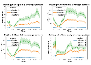
(a) Beijing

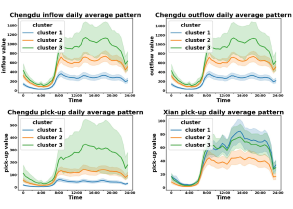
(b) Chengdu and Xi’an

Figure 2: Average daily pattern of taxi service data in (a) Beijing, (b) Chengdu and Xi’an. We aggregate all values at each timestamp from all days, and represent mean values at each timestamp using solid lines, and standard deviations using shades.

A.5 More Machine Learning Benchmarks

A.5.1 Traffic Speed Prediction

RMSE/MAE	Xi’an	Chengdu	Hong Kong
HA	8.7475/5.0312	7.9507/4.5202	6.784/3.8175
LR	8.1432/4.5687	7.4246/4.1844	5.7752/3.3942
GCN	7.5872/4.1807	7.0598/3.9894	5.5043/3.1405
GAT	7.5217/4.0987	6.9622/3.8825	5.5722/3.1465

Table 8: Results for traffic speed prediction in Xi’an, Chengdu, and Hong Kong.

We investigate the traffic speed prediction problem [20, 9]. We formulate the problem as learning a multi-step prediction function $f_{c}(\cdot)$:

$$\left[\tilde{\mathbf{x}}_{c}^{s}(\tau),...,\tilde{\mathbf{x}}_{c}^{s}(\tau+L_{o}-1)\right] =\tilde{f}_{c}\left(\left[\mathbf{x}_{c}^{s}(\tau-L_{i}),...,\mathbf{x}_{c}^{s}(\tau-1)\right]\right),$$ (9)

$$f_{c}=\arg\min_{\tilde{f}_{c}}\sum_{\tau\in\mathcal{T}_{c}} error\left(\tilde{\mathbf{x}}_{c}^{s}\left(\tau\right),\mathbf{x}_{c}^{s}\left(\tau\right)\right),$$

where $\mathbf{x}_{c}^{s}$ is a shorthand for the traffic speed sub-dataset $\mathbf{x}^{speed}_{c}$. In this experiment, the input length $L_{i}$ is set to 12 (2 hours) and the output length $L_{o}$ is set to 6 (1 hour). We investigate four methods, HA, LR, GCN and GAT described in Sec. 4.1.1. For $i,j\in SEG_{c},i=(pos_{0}^{i},pos_{1}^{i}),j=(pos_{0}^{j},pos_{1}^{j})$, the adjacency matrix $\mathbf{A}$ for GNN models is calculated as

$$\mathbf{A}(i,j)=\left\{\begin{array}[]{lr}1,&pos_{0}^{i}=pos_{1}^{j}\text{ or }pos_{1}^{i}=pos_{0}^{j}\\ 0,&\text{otherwise}\end{array}.\right.$$ (10)

Table 8 shows the results of the traffic speed prediction tasks in three cities for all examined models.

A.5.2 Reinforcement Learning

Planning for adequate travel resource allocation is important in smart city. Based on the data in CityNet, we provide benchmarks for the taxi dispatching task, where operators continually dispatch available taxis to waiting passengers in real-time so as to maximize the long-term total revenue of the taxi system.

Problem Statement. Given historical requests from passengers, we learn a real-time taxi dispatching policy. At every timestamp $\tau$, we dispatch available taxis to the current passengers according to the policy so as to maximize the total revenue of all taxis in the long run. Specifically, we divide the city into uniform hexagon grids, instead of square ones hexagon as per previous studies [13, 17].

Methods. We study the following methods for taxi dispatching.

• Greedy is a heuristic algorithm that dispatches the closest available taxi to each passenger one by one.

• LLD is an optimization based approach formulated as Eqn. 11, where $a_{ij}=1$ if taxi $j$ is dispatched to passenger $i$ and 0 otherwise; $A(i,j)$ is the immediate revenue to taxi $j$ after driving passenger $i$ to his/her destination. The definition of the immediate revenue follows [17].

  $$\begin{split}&\max_{a_{ij}}\sum_{i=0}^{m}\sum_{j=0}^{n}A(i,j)a_{ij}\\ &s.t.\left\{\begin{matrix}\sum_{i=0}^{m}a_{ij}=1,j=1,2,3,...,n\\ \\ \sum_{j=0}^{n}a_{ij}=1,i=1,2,3,...,m\end{matrix}\right.\end{split}$$ (11)

• LPA [17] is a reinforcement learning based planning approach. We first adopt SARSA [17] to learn the expected long-term revenue of each grid in each period. Then, based on these expected revenues, we dispatch taxis to passengers by the same optimization formulation as Eqn. 11, except that we replace $A(i,j)$ with the scores learned by SARSA. LPA tries to maximize the total revenue of the system in the long-run instead of immediate revenues.

Experimental Settings

Based on historical request data, we implement a simulator according to [17, 25] to simulate how the taxi system operates, and evaluate these methods on our simulator.

We show taxi dispatching results in Chengdu in Table 9, where Completion rate denotes the ratio of completed requests within all requests, and Accumulated revenue denotes the total revenue received by all taxis in the whole day. We draw the following conclusions from the experiment results:

• Greedy algorithm, which does not consider any global optimization targets, performs the worst compared to LLD and LPA. Taking global optimization targets into consideration leads to an improvement of 5%-20% in completion rate and 2%-8% in revenue.

• LPA performs better than LLD most of the time. Since LPA optimizes the expected long-term revenues at each dispatching round, while LLD only focuses on the immediate reward, LPA should compare favorably against LLD.

Date	Completion rate			Accumulated revenue
	Greedy	LLD	LPA	Greedy	LLD	LPA
Oct. 1st	0.689	0.734	0.718	1,017,144	1,035,724	1,016,410
Oct. 2nd	0.705	0.765	0.752	969,340	984,424	975,157
Oct. 3rd	0.680	0.734	0.747	943,422	961,263	969,341
Oct. 4th	0.695	0.810	0.830	965,896	1,034,539	1,041,978
Oct. 5th	0.708	0.782	0.811	984,225	1,021,727	1,032,165
Oct. 6th	0.735	0.832	0.825	979,356	1,028,292	1,020,174
Oct. 7th	0.774	0.872	0.889	932,641	977,996	980,397

Table 9: Results for taxi dispatching in Chengdu

A.6 Details of Machine Learning Experiments

We provide detailed settings for our machine learning experiments. Note that we only tune these settings to make sure all models converge, rather than to achieve state-of-the-art results.

A.6.1 Taxi Service Prediction

For CNN and LSTM, we train models with learning rate 1e-4, weight decay 0 using Adam optimizer for 75 epochs, and choose the model with the lowest validation error for testing. We set the batch size as 64 for CNN, and use variable batch sizes (Beijing 4, Shanghai 8, Shenzhen/Chongqing 16, Xi’an/Chengdu 32) for LSTM. Weather data are used in training the model following the method in [22]. Each result is an average of 5 independent runs.

A.6.2 Inter-city Transfer Learning

For fine-tuning, we tune the model trained over the source city with learning rate 5e-5, weight decay 0 using Adam optimizer for 100 epochs, and choose the model with the lowest validation error on the target city for testing. For RegionTrans, the weight for feature consistency is taken as 0.01.

A.7 Hardware Configurations and Data-sharing Approaches

All experiments included in this paper are conducted with Python 3.6 and PyTorch 1.6.0 environment on Tesla V100 GPUs. The hardware is affiliated to the Turing AI Computing Cloud (TACC) maintained by the iSING Lab at HKUST.

To empower smart city applications including transportation, healthcare, finance, etc., we are building TACC, an open platform that provides high performance computing resources, massive smart city data including our CityNet, and state-of-the-art machine learning algorithmic paradigms. Researchers can train their own machine learning models on CityNet on TACC equipped with GPUs and RDMA for free. We plan to open the platform to the the academic community in Hong Kong by December 2021, and to the global researchers by June 2022.

A.8 Author statement and license

We bear all responsibility in case of violation of rights during using, processing and distributing these data. This work is licensed under a CC BY 4.0 license.

References

- [1] Chao Chen. Freeway performance measurement system (pems). 2003.
- [2] Nivan Ferreira, Jorge Poco, Huy T Vo, Juliana Freire, and Cláudio T Silva. Visual exploration of big spatio-temporal urban data: A study of new york city taxi trips. IEEE transactions on visualization and computer graphics, 19(12):2149–2158, 2013.
- [3] Xu Geng, Yaguang Li, Leye Wang, Lingyu Zhang, Qiang Yang, Jieping Ye, and Yan Liu. Spatiotemporal multi-graph convolution network for ride-hailing demand forecasting. In Proceedings of the AAAI Conference on Artificial Intelligence, volume 33, pages 3656–3663, 2019.
- [4] H.V. Jagadish, Johannes Gehrke, Alexandras Labrinidis, Yannls Papakonstantinou, Jignesh M. Patel, Raghu Ramakrishnan, and Cyrus Shahabi. Big data and its technical challenges. Communications of the Acm, 57(7):86–94, 2014.
- [5] Thomas N Kipf and Max Welling. Semi-supervised classification with graph convolutional networks. arXiv preprint arXiv:1609.02907, 2016.
- [6] Minne Li, Zhiwei Qin, Yan Jiao, Yaodong Yang, Jun Wang, Chenxi Wang, Guobin Wu, and Jieping Ye. Efficient ridesharing order dispatching with mean field multi-agent reinforcement learning. In The World Wide Web Conference, pages 983–994, 2019.
- [7] Qimai Li, Zhichao Han, and Xiao-Ming Wu. Deeper insights into graph convolutional networks for semi-supervised learning. In Proceedings of the AAAI Conference on Artificial Intelligence, volume 32, 2018.
- [8] Ting Li, Junbo Zhang, Kainan Bao, Yuxuan Liang, Yexin Li, and Yu Zheng. Autost: Efficient neural architecture search for spatio-temporal prediction. In Proceedings of the 26th ACM SIGKDD International Conference on Knowledge Discovery & Data Mining, pages 794–802, 2020.
- [9] Yaguang Li, Rose Yu, Cyrus Shahabi, and Yan Liu. Diffusion convolutional recurrent neural network: Data-driven traffic forecasting. arXiv preprint arXiv:1707.01926, 2017.
- [10] Binbing Liao, Jingqing Zhang, Chao Wu, Douglas McIlwraith, Tong Chen, Shengwen Yang, Yike Guo, and Fei Wu. Deep sequence learning with auxiliary information for traffic prediction. In Proceedings of the 24th ACM SIGKDD International Conference on Knowledge Discovery and Data Mining. ACM, 2018.
- [11] Wei Liu, Yu Zheng, Sanjay Chawla, Jing Yuan, and Xie Xing. Discovering spatio-temporal causal interactions in traffic data streams. In Proceedings of the 17th ACM SIGKDD international conference on Knowledge discovery and data mining, pages 1010–1018, 2011.
- [12] Sinno Jialin Pan and Qiang Yang. A survey on transfer learning. IEEE Transactions on knowledge and data engineering, 22(10):1345–1359, 2009.
- [13] Xiaocheng Tang, Zhiwei (Tony) Qin, Fan Zhang, Zhaodong Wang, Zhe Xu, Yintai Ma, Hongtu Zhu, and Jieping Ye. A deep value-network based approach for multi-driver order dispatching. In Proceedings of the 25th ACM SIGKDD International Conference on Knowledge Discovery and Data Mining, pages 1780–1790, 2019.
- [14] Petar Veličković, Guillem Cucurull, Arantxa Casanova, Adriana Romero, Pietro Lio, and Yoshua Bengio. Graph attention networks. arXiv preprint arXiv:1710.10903, 2017.
- [15] Leye Wang, Xu Geng, Xiaojuan Ma, Feng Liu, and Qiang Yang. Cross-city transfer learning for deep spatio-temporal prediction. In Proceedings of the 28th International Joint Conference on Artificial Intelligence, pages 1893–1899. AAAI Press, 2019.
- [16] Ying Wei, Yu Zheng, and Qiang Yang. Transfer knowledge between cities. In Proceedings of the 22nd ACM SIGKDD International Conference on Knowledge Discovery and Data Mining, pages 1905–1914, 2016.
- [17] Zhe Xu, Zhixin Li, Qingwen Guan, Dingshui Zhang, Qiang Li, Junxiao Nan, Chunyang Liu, Wei Bian, and Jieping Ye. Large-scale order dispatch in on-demand ride-hailing platforms: A learning and planning approach. In Proceedings of the 24th ACM SIGKDD International Conference on Knowledge Discovery and Data Mining, pages 905–913, 2018.
- [18] Qiang Yang, Yang Liu, Tianjian Chen, and Yongxin Tong. Federated machine learning: Concept and applications. ACM Transactions on Intelligent Systems and Technology (TIST), 10(2):1–19, 2019.
- [19] Huaxiu Yao, Yiding Liu, Ying Wei, Xianfeng Tang, and Zhenhui Li. Learning from multiple cities: A meta-learning approach for spatial-temporal prediction. In The World Wide Web Conference, pages 2181–2191, 2019.
- [20] Bing Yu, Haoteng Yin, and Zhanxing Zhu. Spatio-temporal graph convolutional networks: a deep learning framework for traffic forecasting. In Proceedings of the 27th International Joint Conference on Artificial Intelligence, pages 3634–3640, 2018.
- [21] Jing Yuan, Yu Zheng, Xing Xie, and Guangzhong Sun. Driving with knowledge from the physical world. In Proceedings of the 17th ACM SIGKDD international conference on Knowledge discovery and data mining, pages 316–324, 2011.
- [22] Junbo Zhang, Yu Zheng, and Dekang Qi. Deep spatio-temporal residual networks for citywide crowd flows prediction. In Proceedings of the AAAI Conference on Artificial Intelligence, volume 31, 2017.
- [23] Junbo Zhang, Yu Zheng, Dekang Qi, Ruiyuan Li, and Xiuwen Yi. Dnn-based prediction model for spatio-temporal data. In Proceedings of the 24th ACM SIGSPATIAL International Conference on Advances in Geographic Information Systems, pages 1–4, 2016.
- [24] Yu Zheng, Licia Capra, Ouri Wolfson, and Hai Yang. Urban computing: concepts, methodologies, and applications. ACM Transactions on Intelligent Systems and Technology (TIST), 5(3):1–55, 2014.
- [25] Ming Zhou, Jiarui Jin, Weinan Zhang, Zhiwei Qin, Yan Jiao, Chenxi Wang, Guobin Wu, Yong Yu, and Jieping Ye. Multi-agent reinforcement learning for order-dispatching via order-vehicle distribution matching. In Proceedings of the 28th ACM International Conference on Information and Knowledge Management, pages 2645–2653, 2019.
Acknowledgments and Disclosure of Funding
This project is sponsored by RGC Theme-based Research Scheme (No.T41-603/20R). The raw datasets are retrieved from Didi Chuxing GAIA Initiative (https://gaia.didichuxing.com) and some other open-source channels. We appreciate the effort from Hao Liu, Kaiqiang Xu and Xiaoyu Hu ({liuh,kxuar,huxiaoyu}@ust.hk, HKUST) throughout this research work.