Monocular 3D Object Detection: An Extrinsic Parameter Free Approach

Abstract

Monocular 3D object detection is an important task in autonomous driving. It can be easily intractable where there exists ego-car pose change w.r.t. ground plane. This is common due to the slight fluctuation of road smoothness and slope. Due to the lack of insight in industrial application, existing methods on open datasets neglect the camera pose information, which inevitably results in the detector being susceptible to camera extrinsic parameters. The perturbation of objects is very popular in most autonomous driving cases for industrial products. To this end, we propose a novel method to capture camera pose to formulate the detector free from extrinsic perturbation. Specifically, the proposed framework predicts camera extrinsic parameters by detecting vanishing point and horizon change. A converter is designed to rectify perturbative features in the latent space. By doing so, our 3D detector works independent of the extrinsic parameter variations and produces accurate results in realistic cases, e.g., potholed and uneven roads, where almost all existing monocular detectors fail to handle. Experiments demonstrate our method yields the best performance compared with the other state-of-the-arts by a large margin on both KITTI 3D and nuScenes datasets.

1 Introduction

3D object detection plays an important role in a variety of computer vision tasks, such as automated driving vehicles, autonomous drones, robotic manipulation, augmented reality applications, etc. Most existing 3D detectors require accurate depth-of-field information. To acquire such resource, majority of the methods resort to the LiDAR pipeline [10, 33, 37, 38, 23, 60], some to the radars solution [27, 54, 18, 20] or others to the multi-camera framework [8, 9, 21, 32, 35, 51]. In this paper, we address this problem in a monocular camera setting and curate it specifically for automated driving scenarios With the difficulty in directly acquiring a depth of field information, monocular 3D detection (Mono3D) is an ill-posed and challenging task. However, Mono3D approaches have the advantage of low cost, low power consumption, and easy-to-deployment in real-world applications. Therefore, monocular 3D detection has received increasing attention over the past few years [2, 7, 28, 29, 34, 39].

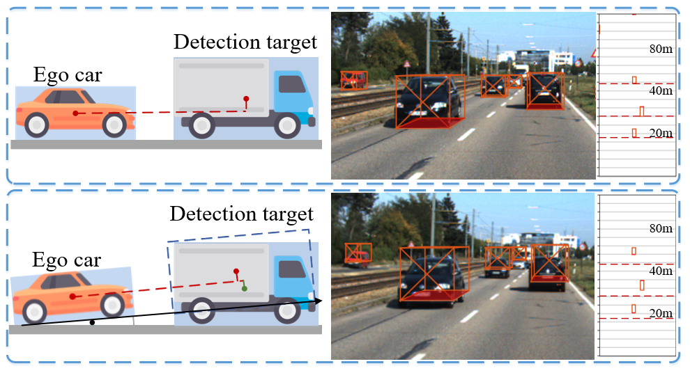
Figure 1: The effect of extrinsic parameter perturbations on 3D detection task. When the vehicle undergoes a slight pose change on an uneven road, the 3D detection results are less accurate (second row). This happens often in realistic applications and the detection offset can be viewed more evidently in the bird-eye’s view.

Current Mono3D methods have achieved considerable high accuracy given a specifically fixed camera coordinate system. However, in real scenarios, the unevenness (perturbation) of the road surface often causes the camera extrinsic parameters to be disturbed, which introduces a significant algorithmic challenge. To the best of our knowledge, there are no 3D detection datasets that takes into account the camera pose change under perturbation.

As shown in Figure 1, current datasets or detectors assume there is no perturbation, i.e., the extrinsic parameters are set to be constant. Therefore the accurate 3D results are obtained (top row). However, as depicted in the bottom perturbation case, the object information viewed by the camera deviates from the real object information. This makes the detection results unreliable by recovering a large offset in form of both 3D boxes and bird-eye’s view. Straightforward methods to address this problem are to design complementary branches or networks to improve the generalization ability, and yet this solution yields limited improvement [5, 50, 34, 45, 12]. Some approaches utilize vehicle CAD models or keypoints to reconstruct vehicle geometry [5, 50], while others exploit existing networks to predict pixel-level or instance-level depth map by mimicking state-of-the-art (SOTA) LiDAR 3D detection methods, namely pseudo-LiDAR methods [34, 45, 12].

Our work is inspired by the visual odometry methods that resolve camera pose change in adjacent frames from images [16, 22, 36, 46, 56, 58]. Note that this idea differentiates from those that focus solely on detecting objects in the perturbation-prone camera coordinate system [39, 2, 24, 59, 11, 42, 3]. These approaches focus on some less critical issues regarding to realistic industrial applications. For example, the modeling of occlusive objects [11], depth branches [42], kinematic motion information (object orientation) [3], etc. Moreover, it is similar to human behavior patterns that one can naturally adapt to changing road gradients and gradually deduce the accurate position of objects even on potholes. Formulating our network to encode such learning patterns is feasible on a biological basis.

In this paper, we propose to leverage the extrinsic parameter change implicitly in the image. Our key idea is to estimate camera pose change w.r.t. the ground plane from images and optimize predicted 3D locations of objects guided by the camera extrinsic geometry constraint. We abbreviate the proposed framework as MonoEF (extrinsic parameter free detector). Specifically, a novel detector is proposed to extract the vanishing point and horizon information from the image to estimate the camera extrinsic corresponding to the image. The model is thus capable of capturing the extrinsic parameter perturbations to which the current image is subjected in the geometric space. During inference, we transform latent feature space using extrinsic parameters as seed to remove the effect of extrinsic perturbations on features fed from the input image. Note that the transformation network is learned in a supervised manner, which allows the image features to recover from camera perturbation. By doing so, we impose our detector exclusive from the effects of the extrinsic parameter. The resultant 3D locations are obtained via the extrinsic parameter-free predictor and projected back into the real-world coordinate system.

Experiments on both the KITTI 3D benchmark [15] and nuScenes dataset [4] demonstrate that our method outperforms the SOTA methods by a large margin, especially for perturbative examples with a distinguished improvement. To sum up, the contributions of our paper are as follows:

• We introduce a novel Mono3D detector by capturing the perturbative information of the extrinsic parameters from monocular images to make the detector free from extrinsic fluctuation.

• We design a feature transformation network, using camera extrinsic parameters as seed, to recover the non-perturbative image information from the perturbative latent feature space.

• We propose an extrinsic module that complements the camera’s pose in 3D object detection. Such a plug-and-play can be applied to existing detectors and pragmatic for industrial applications, e.g., autonomous driving scenarios.

The whole suite of the codebase will be released and the experimental results will be pushed to the public leaderboard.

2 Related Work

Monocular 3D Object Detection.   The Monocular camera is in lacks 3D information compared with multi-beam LiDAR or stereo cameras. To overcome this difficulty and reconstruct the geometry and position of the object in world coordinates, most Mono3D methods can be roughly divided into three categories. In the first category [7, 31, 5], auxiliary information is widely used like vehicle Computer-Aided Design (CAD) models or keypoints. By this means, extra labeling cost is inevitably required. In the second category [26, 28, 49, 51], the prior knowledge like depth map by LiDAR point cloud, or disparity map by stereo cameras trained by external data is exploited. Usually, the inference time would increase significantly due to the prediction of these dense heat maps.

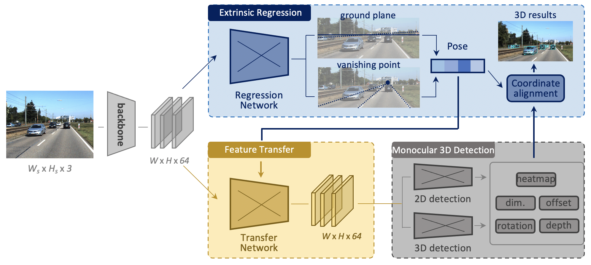
Figure 2: System overview. The Extrinsic Regression module (blue block) predicts the ground plane as well as vanishing point. The pose information is thereby obtained and then fed into the Feature Transfer module (yellow block) as guidance for feature enhancement. By doing so, the original features (in gray color) after the backbone are transferred to a rectified set of features (in yellow color), immune to the extrinsic parameter perturbation. The Monocular 3D Detection module and coordinate alignment unit follow standard procedures [24].

Unlike the aforementioned work, methods in the third category only make use of the RGB image as input and remove the dependencies on extra labeling or pre-trained networks by external data. SMOKE [24] predicts a 3D bounding box by combining a single keypoint estimation with regressed 3D variables based on CenterNet [59]. M3D-RPN [2] reformulates the monocular 3D detection problem as a standalone 3D region proposal network. Current SOTA results for monocular 3D object detection are from MonoPair [11], Center3D [42], and Kinematic3D [3]. Among them, MonoPair [11] improves the modeling of occlusive objects by considering the relationship of paired samples. Center3D [42] carefully designs two modules for better depth prediction called LID and DepJoint. Kinematic3D [3] proposes a novel method for monocular video-based 3D object detection which leverages kinematic motion to improve the precision of 3D localization.

However, all the object detectors mentioned above focus only on the information in the current camera coordinate system that ignores the effect of camera pose on detection. These methods do not work well when the camera’s pose receives a disturbance w.r.t. ground plane due to rough terrain or acceleration of ego vehicle.

Deep Monocular Odometry.   With the success of deep neural networks, end-to-end learning-based methods [47, 48, 52, 53] have been proposed to tackle the visual odometry problem. Recently, some methods [1, 41, 43, 44, 57] exploit CNNs to predict the scene depth and camera pose jointly, utilizing the geometric connection between the structure and the motion. This corresponds to learning Structure-from-Motion (SfM) in a supervised manner. To mitigate the requirement of data annotations, self-supervised and un-supervised methods [16, 22, 36, 46, 56, 58] have been proposed to tackle the SfM task. CC [36] addresses the unsupervised learning of several interconnected problems in low-level vision: single view depth prediction, camera motion estimation, optical flow, and segmentation of a video into the static scene and moving regions. MonoDepth2 [16] proposes a set of improvements, which together result in both quantitatively and qualitatively improved depth maps compared to competing for self-supervised methods. LTMVO [61] presents a self-supervised learning method for visual odometry with special consideration for consistency over longer sequences.

While these visual odometry methods are relatively good at detecting camera pose, they all rely on motion information on the time series, which will not be available in a typical Mono3D task based on single-frame images. Consequently, the lack of motion information in the time series prevents us from directly obtaining accurate camera pose information. However, We can still use similar ideas to detect changes in the ground plane and vanishing point from the image compared to the reference frame, and thus indirectly infer changes in the camera extrinsic parameters.

3 An Extrinsic Parameter Free Approach

3.1 Overview

We adopt the one-stage anchor-free architecture as does in SMOKE [24]. Figure 2 depicts an overview of our framework. It contains a backbone network, an extrinsic regression network, a feature transfer network, and several task-specific dense prediction branches. The backbone takes a monocular image of size $(W_{s}\times H_{s}\times 3)$ as input and outputs a feature map of size $(W\times H\times 64)$ after down-sampling with an s-factor. The feature map is utilized for extrinsic parameter detection (top blue pipeline), and in parallel rectified by the transfer network based on extrinsic parameters (known as Pose as in the bottom yellow pipeline). For 2D and 3D detection, we follow standard procedures in this domain. There exist seven output branches with each having size of $(W\times H\times m)$, where $m$ is the output channel of each branch. The detection results need to be aligned by the predicted extrinsic parameters in order to get the final bounding box and position.

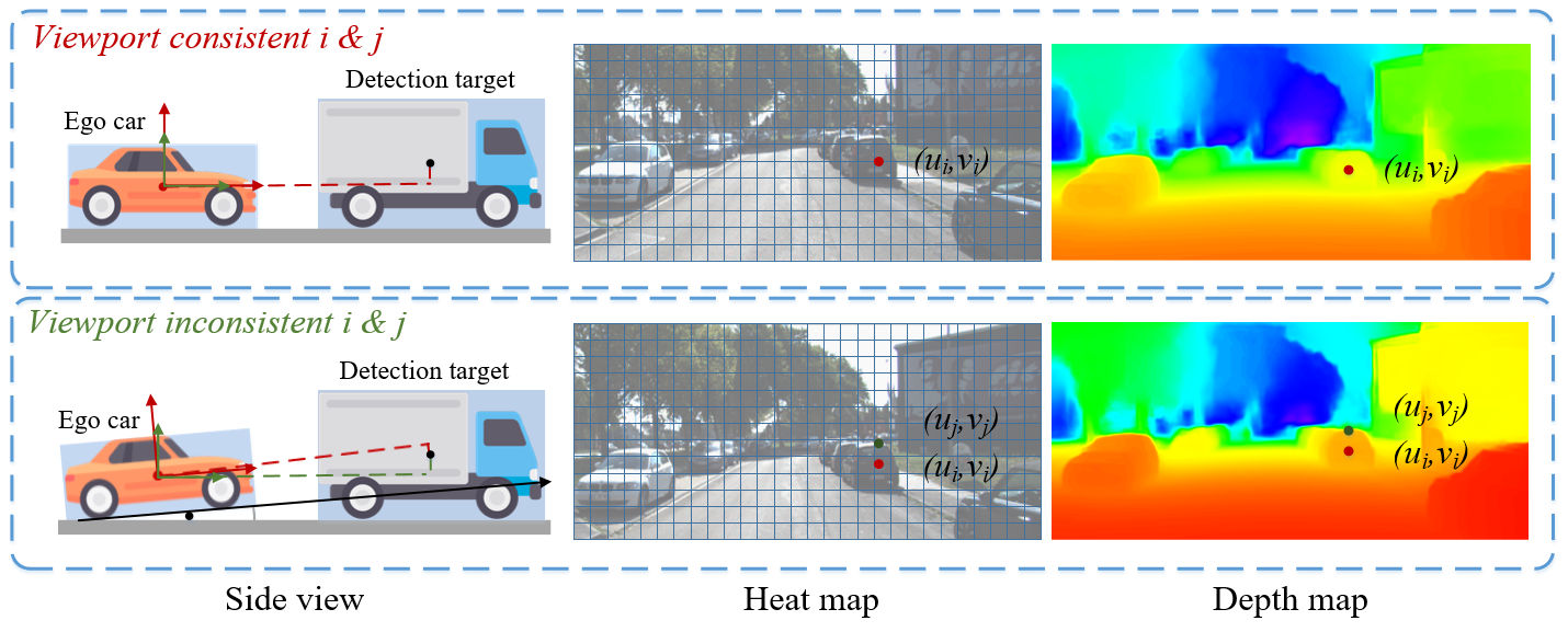
Figure 3: Visualization of the extrinsic perturbation. The pose of the ego vehicle varies due to the unevenness of road surfaces, which is quite common in realistic scenarios. It causes the camera’s viewport $i$ to be inconsistent with ground viewport $j$. Therefore, the position of keypoints found from the heat map and depth map are shifted from $(u_{i},v_{i})$ to $(u_{j},v_{j})$ by extrinsic perturbation, leading to a confusion for the 3D prediction and thereby inaccurate results.

3.2 Preliminary on Monocular Object Detection

The 2D object detection follows the design of CenterNet [59]. A heatmap of size $(W\times H\times c)$ is used to enable keypoint localization$(u^{g},v^{g})$ and its classification. The number of object categories $c$ equals three on KITTI3D benchmark and ten on nuScenes dataset. The other two branches of size $(W\times H\times 2)$ are adopted to regress the dimensions of the 2D bounding box $(w^{b},h^{b})$ and the offset $(\delta^{u},\delta^{v})$ from the center of the bounding box $(u^{b},v^{b})$ to the keypoint $(u^{g},v^{g})$ correspondingly.

The 3D object detection focuses on the 3D information of an object in the local camera coordinate system instead of the global world coordinate system. The object center in local camera coordinate system can be represented as homogeneous coordinates $\mathbf{c}^{w}=(x,y,z)$; its projection in the feature map is $\mathbf{c}^{o}=(u,v,1)$. Similar to [28, 39], we predict the offset $(\Delta^{u},\Delta^{v})$ to the keypoint location $(u^{g},v^{g})$ and depth $z$ in two separate branches. Denote the coordinates in form of congruent concept, we have:

$$z\left[\begin{matrix}u\ v\ 1\end{matrix}\right]^{T}=\mathbf{P}\cdot\left[\begin{matrix}x\ y\ z\end{matrix}\right]^{T},$$ (1)

where $\mathbf{P}$ is the projection conversion matrix between the world coordinate system and the image coordinate system. The projection matrix can be decomposed as:

$$\mathbf{P}=\mathbf{K}\cdot\mathbf{T},$$ (2)

where $\mathbf{K}$ is referred to as the constant camera intrinsic matrix and $\mathbf{T}$ as the inconstancy extrinsic matrix w.r.t ground plane. Naturally we have $\mathbf{c}^{o}=\frac{1}{z}\mathbf{P}\mathbf{c}^{w}$. The depth $z$ and size $(w,h,l)$ are regressed according to [13]. As aforementioned in Section 3.1, in these branches, the regression components are trained with the L1 loss. Similar to [29, 59], we represent the orientation using eight scalars, where the orientation branch is trained using the multi-bin loss [30].

3.3 Theoretical Analysis

Figure 3 depicts a concrete example of how an extrinsic perturbation can significantly impose poor prediction onto heat map and depth map.

Given a specific local camera coordinate system called viewport $i$, it is normally assumed that the viewport $i$ is consistent with ground plane coordinate system called viewport $j$, so do most of Mono3D datasets. Suppose the 3D center of a selected object in viewport $i$ is $\mathbf{c}_{i}^{w}=(x_{i},y_{i},z_{i})$, and the 3D center on the feature map is $\mathbf{c}_{i}^{o}=(u_{i},v_{i},1)$, corresponding to the case as depicted in Figure 3. If there is an extrinsic perturbation from the ground plane variation, the identical relation between camera viewport $i$ and ground plane viewport $j$ would no longer exist. We discriminate this process as perturbation. The perturbation matrix $\mathbf{A}$ can be described as:

$$\mathbf{A}=\left[\begin{matrix}\cos\theta_{r}&\sin\theta_{r}&0\\ \cos\theta_{p}\sin\theta_{r}&\cos\theta_{r}\cos\theta_{p}&\sin\theta_{p}\\ -\sin\theta_{p}\sin\theta_{r}&-\sin\theta_{p}\cos\theta_{r}&\cos\theta_{p}\end{matrix}\right],$$ (3)

where $\theta_{p}$ stands for pitch angle and $\theta_{r}$ for roll angle of ego vehicle w.r.t. ground plane respectively. Now we are equipped with the extrinsic perturbation being introduced spatially, the center of the object $\mathbf{c}_{i}^{w}$ of camera viewport $i$ is transformed to a point $\mathbf{c}_{j}^{w}$ in the ground plane viewport $j$, where $\mathbf{c}_{j}^{w}=z_{j}\mathbf{P}_{j}^{-1}\mathbf{c}_{j}^{o}=\mathbf{A}\mathbf{c}_{i}^{w}$. On the feature map, the keypoint of the object shifts correspondingly from $\mathbf{c}_{i}^{o}$ to $\mathbf{c}_{j}^{o}$. The transfer relationship matrix $\mathbf{M}$ of keypoints on the feature map can be represented by:

$$\mathbf{c}_{j}^{o}=\mathbf{M}\mathbf{c}^{o}_{i}=\frac{z_{i}}{z_{j}}\mathbf{P}_{j}\mathbf{A}\mathbf{P}_{i}^{-1}\mathbf{c}_{i}^{o}.$$ (4)

This shift in image coordinates would cause confusion for the prediction of 3D position.

Given the example in Figure 3, we use the changes on the depth hidden map to perform our analysis. If the model can know the changes that occur in the ground plane coordinate system, such as LiDAR-based methods, it will assume that the target has changed in height. However, for the camera, the height and depth of the target will both affect its position on the image. The camera assumes that the target vehicle remains on the ground coordinate system at all times, so it incorrectly determines that the change in the target on the image is caused by the depth. The offset of keypoints leads to large depth prediction errors.

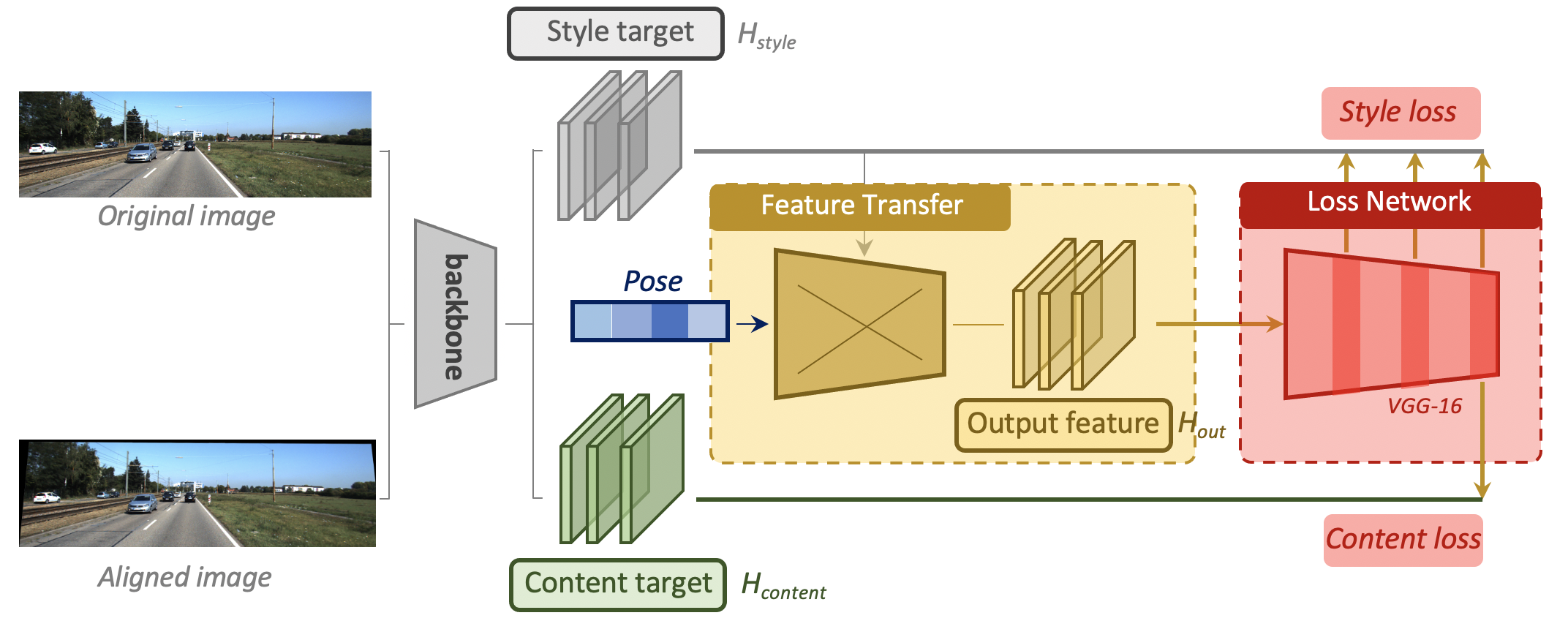
Figure 4: The training process of the transfer network $f^{t}$. The feature target is derived from a feature obtained by the backbone after a direct extrinsic parameter correction of the image. The pre-trained loss network $\Phi$ has two branches, one with the style target for high-dimensional losses computed on three layers and the other with the content target for low-dimensional losses computed only on the last layer.

These keypoint positions need to be rectified to compensate for offsets caused by the change of camera extrinsic parameter. For training, $\mathbf{A}$ in Equation (3) can be collected through the ground truth vehicle ego-pose information. The image feature w.r.t. viewport $\mathbf{H}_{j}$ and labels $\mathbf{c}_{j}^{w}$ need to be first adjusted using matrices $\mathbf{M}^{-1}$ and $\mathbf{A}^{-1}$ separately in order to eliminate the effect of extrinsic perturbations $\mathbf{A}$. The label obtained by 3D detector $f^{\theta_{i}}$ established at camera viewport $i$ can be recorded as $\hat{\mathbf{c}}_{i}^{w}$. The L1 loss function under external parameter perturbation is changed to

$$\begin{split}\hat{\mathbf{c}}_{i}^{w}&=f^{\theta_{i}}(f^{t}(\mathbf{M}^{-1},\mathbf{H}_{j}))=f^{\theta_{i}}(\mathbf{H}_{i}),\\ L(\theta_{j})&=\left\|\mathbf{A}^{-1}\mathbf{c}_{j}^{w}-\hat{\mathbf{c}}_{i}^{w}\right\|=\left\|\mathbf{c}_{i}^{w}-\hat{\mathbf{c}}_{i}^{w}\right\|,\end{split}$$ (5)

where $f^{t}(\cdot,\cdot)$ is the transfer network on the feature implicit space which maps the change on camera extrinsic parameters to the feature map.

During inference, we first estimate camera extrinsic parameters $\hat{\mathbf{A}}$ from input image $\mathbf{X}_{j}$ and recover the unperturbed feature hidden space $\hat{\mathbf{H}}_{i}$ from the perturbed feature hidden space $\mathbf{H}_{j}$ using $\hat{\mathbf{M}}$. The predicted 3D center $\hat{\mathbf{c}}_{j}^{w}$ is derived from the 3D detector $f^{\theta_{i}}$ which is independent of varying camera extrinsic parameters $\hat{\mathbf{A}}$:

$$\hat{\mathbf{c}}_{j}^{w}=\hat{\mathbf{A}}f^{\theta_{i}}(f^{t}(\hat{\mathbf{M}}^{-1},\hat{\mathbf{H}}_{j}))=\hat{\mathbf{A}}f^{\theta_{i}}(\hat{\mathbf{H}}_{i})).$$ (6)

For camera extrinsic parameters $\mathbf{A}$ and $\mathbf{M}$, we propose the extrinsic regression network, which is introduced in Section 3.4. For feature transfer network $f^{t}$, the design methodology and training process is described in Section 3.5. These modules are utilized to detect extrinsic perturbations of the image in viewport $j$, and further adopt the extrinsic information to rectify the feature map. In this way, the image features can be restored back to camera viewport $i$, and the 3D detection model no longer receives the negative impact from extrinsic perturbations.

3.4 Camera Extrinsic Parameters Regression

In addition to the regular regression task, we also introduce a module of extrinsic parameter regression in Mono3D branches, which is shown in Figure 2.

Owing to the fact that extrinsic parameters are too implicit for a model to regress, we choose to predict intuitive and explicit features from the image at first. The horizon and vanishing point in the image are often used to help determine the vehicle’s ego-pose information w.r.t ground plane in the deep visual odometry tasks. Specifically, the tilt of the horizon can indicate the change of roll angle, while the vertical movement of the vanishing point can indicate the change of pitch angle.

Following the SOTA odometry framework in [6], we represent a regression task with L1 loss as:

$$\begin{split}[\hat{\mathbf{y}}_{\mathrm{gp}},\hat{\mathbf{y}}_{\mathrm{vp}}]&=f^{\mathrm{vo}}(\mathbf{H}_{j}),\\ L_{\mathrm{vo}}&=\left\|\mathbf{A}-\mathbf{g}(\hat{\mathbf{y}}_{\mathrm{gp}},\hat{\mathbf{y}}_{\mathrm{vp}})\right\|.\end{split}$$ (7)

Here, $f^{\mathrm{vo}}$ is the CNN architecture used for horizon and vanishing point detection, we follow [19] and make modifications to the filters for the fully connected layers. $\hat{\mathbf{y}}_{\mathrm{gp}}$ and $\hat{\mathbf{y}}_{\mathrm{vp}}$ are the predicted ground plane and vanishing point results at viewport $j$. The mapping function $\mathbf{g}:(\mathbb{R}^{2},\mathbb{R}^{2})\mapsto\mathbf{A}_{4\times 4}$ is a mathematical calculation function from the horizon and vanishing point to the camera extrinsic matrix. The function $f^{\mathrm{vo}}$ ensures that the model can give sufficiently accurate information about the extrinsic parameters. Finally, the regression loss $L_{\mathrm{vo}}$ can be trained jointly with 2D and 3D detection branches.

3.5 Feature Transfer by Extrinsic Parameters

To overcome the pose variation of ego vehicle w.r.t ground plane and improve 3D detection performance, we propose a transfer network applying camera extrinsic corrections on the feature latent layers. Generally speaking, as shown in Figure 3, the design intention of the transfer network is to rectify the perturbed feature space $\mathbf{H}_{j}$ in camera view $j$, so that the discrepancy between $\mathbf{H}_{j}$ and the unperturbed one $\mathbf{H}_{i}$ under camera view $i$ is as small as possible. For example, we fix the shift of keypoints caused by extrinsic parameter perturbations. Suppose that in one image with unknown perturbation, the network predicts camera extrinsic parameters $\hat{\mathbf{A}}=\mathbf{g}(f^{\mathrm{vo}}(\mathbf{H}_{j}))$ based on the strategy in Section 3.4.

After carefully analyzing the influence of perturbation on the image characteristics of low-dimensional features and high-dimensional features, we find out that their changing patterns are quite different. On the one hand, low-dimensional features like the position of corresponding edges and geometries are closely related to the camera’s extrinsic parameters, specifically in terms of content information. On the other hand, high-dimensional features like the textures and illuminations remain unchanged, specifically in terms of style information. Inspired by the image style transfer method [17], we propose a feature transfer module working on the feature latent space.

Methods	$AP_{3D}$			$AP_{BV}$			$AOS$			$AP_{2D}$			Time
	E	M	H	E	M	H	E	M	H	E	M	H
M3D-RPN [2]	14.76	9.71	7.42	21.02	13.67	10.23	88.38	82.81	67.08	89.04	85.08	69.26	0.16
SMOKE [24]	14.03	9.76	7.84	20.83	14.49	12.75	92.94	87.02	77.12	93.21	87.51	77.66	0.03
MonoPair [11]	13.04	9.99	8.65	19.28	14.83	12.89	91.65	86.11	76.45	96.61	93.55	83.55	0.06
PatchNet [25]	15.68	11.12	10.17	22.97	16.86	14.97	-	-	-	93.82	90.87	79.62	0.40
D4LCN [12]	16.65	11.72	9.51	22.51	16.02	12.55	90.01	82.08	63.98	90.34	83.67	65.33	0.20
Kinematic3D [3]	19.07	12.72	9.17	26.69	17.52	13.1	58.33	45.5	34.81	89.67	71.73	54.97	0.12
MonoEF	21.29	13.87	11.71	29.03	19.7	17.26	96.19	90.65	82.95	96.32	90.88	83.27	0.03

Table 1: $AP_{40}$ scores(%) and runtime(s) on KITTI3D test set for car at 0.7 IoU threshold referred from the KITTI benchmark website. E, M and H represent Easy , Moderate and Hard samples. Our model not only ranks first on the 3D evaluation metrics but also keeps the run time fairly low and comparable as a simple one-stage detection. Corner information might be cropped and padded by feature transferring and correction so that the performance of 2D detection is slightly affected.

As shown in Figure 4, this module is divided into two parts. One is the transfer network $f^{t}$, and the other is a pre-trained loss network $\Phi$ using [40].

The transfer network. The input feature map $\mathbf{H}_{\mathrm{in}}$ for transfer network is provided by the previous backbone, which is equal to $\mathbf{H}_{j}$. The predicted pose $\hat{\mathbf{M}}$ acts as a guidance information for transfer network, which provides structural information for feature maps in low dimensions. The output of transfer network $\mathbf{H}_{\mathrm{out}}$ will be input into loss network with content target $\mathbf{H}_{\mathrm{content}}=f^{b}(\hat{\mathbf{M}}^{-1}\mathbf{X}_{j})$ and style target $\mathbf{H}_{\mathrm{style}}=\mathbf{H}_{j}$ to calculate final features, where $\mathbf{X}_{j}$ stands for disturbed image input, and $f^{b}$ stands for backbone network.

The loss network. The transfer network $f^{t}$ mainly considers content loss $l_{\mathrm{content}}$ and style loss $l_{\mathrm{style}}$. Let $\phi_{m}$ be the activation of the $m$-th layer of the network $\Phi$ with the feature map of shape $(c_{m}\times h_{m}\times w_{m})$. The content feature reconstruction loss is the squared Euclidean distance between feature representations:

$$l^{\phi,m}_{\mathrm{content}}(\mathbf{H}_{\mathrm{out}},\mathbf{\mathbf{H}}_{\mathrm{content}})=\frac{\left\|\phi_{m}(\mathbf{H}_{\mathrm{out}})-\phi_{m}(\mathbf{H}_{\mathrm{content}})\right\|_{2}^{2}}{c_{m}h_{m}w_{m}}.$$ (8)

Following [14], we define the $Gram\ matrix\ G^{\phi}_{m}$ to be the $c_{m}\times c_{m}$ matrix whose elements are given by:

$$G^{\phi}_{m}(\mathbf{H})_{c,c^{\prime}}=\frac{\sum^{h_{m}}_{h=1}\sum^{w_{m}}_{w=1}\phi_{m}(\mathbf{H})_{h,w,c}\phi_{m}(\mathbf{H})_{h,w,c^{\prime}}}{c_{m}h_{m}w_{m}}.$$ (9)

The Gram matrix can be computed by reshaping $\phi_{m}(\mathbf{H})$ into a matrix $\psi$, then $G^{\phi}_{m}(\mathbf{H})=\psi\psi^{T}/c_{m}h_{m}w_{m}$. The style reconstruction loss is then the squared Frobenius norm of the difference between the Gram matrices of the output and target feature maps:

$$\l^{\phi,m}_{\mathrm{style}}(\mathbf{H}_{\mathrm{in}},\mathbf{H}_{\mathrm{style}})=\left\|G^{\phi}_{m}(\mathbf{H}_{\mathrm{in}})-G^{\phi}_{m}(\mathbf{H}_{\mathrm{style}})\right\|_{F}^{2}.$$ (10)

The $l_{\mathrm{content}}$ penalizes the output feature map when it deviates in content from the target and $l_{\mathrm{style}}$ penalizes differences in style. The joint total loss is defined as:

$$L_{\mathrm{total}}=\gamma_{1}l_{\mathrm{content}}+\gamma_{2}l_{\mathrm{style}},$$ (11)

where $\gamma_{1}$ and $\gamma_{2}$ are hyper-parameters for tuning content loss and style loss.

Methods	Test Data	$AP_{3D}$			$AP_{BV}$			$AP_{2D}$
		E	M	H	E	M	H	E	M	H
M3D-RPN [2]	original	64.91	50.53	41.73	69.28	53.64	45.12	91.88	93.11	77.24
	disturbed	39.72	31.08	25.73	48.37	38.55	32.22	92.20	93.14	77.13
	decrease	-25.19	-19.45	-16.00	-20.91	-15.09	-12.9	0.32	0.03	-0.11
SMOKE [24]	original	77.89	72.80	65.37	83.30	82.92	75.76	99.50	99.05	90.55
	disturbed	42.58	35.09	30.74	53.01	44.15	39.41	98.66	98.12	89.84
	decrease	-35.31	-37.71	-34.63	-30.29	-38.77	-36.35	-0.85	-0.92	-0.71
D4LCN [12]	original	61.54	45.60	37.77	68.32	51.68	39.31	97.35	89.1	71.51
	disturbed	41.77	29.22	25.78	59.9	43.45	36.06	85.38	76.64	60.03
	decrease	-19.77	-16.38	-11.99	-8.42	-8.23	-3.25	-11.97	-12.46	-11.48
Kinematic3D [3]	original	55.45	39.47	31.29	61.72	44.65	34.58	98.61	86.3	71.39
	disturbed	27.30	16.95	13.79	47.78	36.70	29.24	90.84	55.13	44.80
	decrease	-28.15	-22.52	-17.50	-13.94	-7.95	-5.34	-7.77	-31.17	-26.59
MonoEF	original	77.55	72.83	72.01	82.33	82.80	75.61	99.56	99.19	90.62
	disturbed	76.87	70.86	63.86	81.64	74.76	73.92	99.65	99.15	90.62
	decrease	-0.68	-1.97	-8.16	-0.68	-8.04	-1.70	0.09	-0.04	-0.01

Table 2: $AP_{40}$ scores(%) on KITTI3D validation set for car at 0.5 IoU threshold before and after camera extrinsic disturbance. The lower the decreased value, the better the performance. The original target coordinates are transformed according to the pitch and roll angle set by the artificial extrinsic perturbation. The input image is also processed using the projection transformation according to these angles.

4 Experimental Results

4.1 Implementation Setup

We conduct experiments on the KITTI3D object detection dataset, KITTI odometry dataset and nuScenes dataset. The KITTI3D dataset does not collect camera extrinsic information, which means its $\mathbf{T}$ matrix is an identity matrix. We can only find vehicle ego-pose information from the KITTI odometry and nuScenes datasets.

For the evaluation and ablation study, we show experimental results from two different setups. Baseline is derived from SMOKE [24] with an additional output branch for camera extrinsic parameters. MonoEF is the final proposed method integrating seven prediction branches, camera extrinsic parameter regression branch, and camera extrinsic amendment network.

For the rest of the detailed dataset statistics, training and inference structure, learning rules, evaluation metrics, etc., please refer to the supplementary.

4.2 Quantitative and Qualitative Results

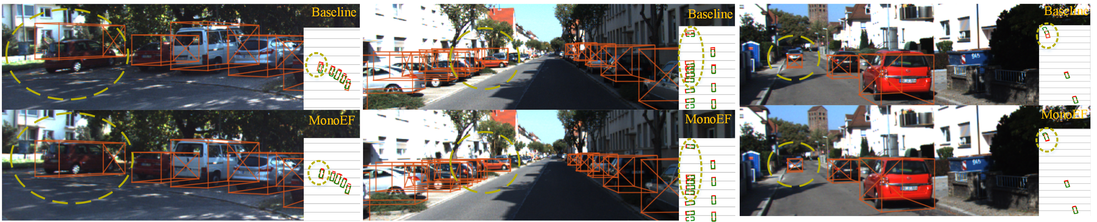
Figure 5: Qualitative results on KITTI odometry dataset. The prediction 3D bounding boxes of SMOKE (the one above) and our model (the one below) are shown under camera extrinsic perturbation in the images. Green boxes and orange boxes in bird view mean ground truth and predictions of cars. A more pronounced difference in the predictions appears where the dashed line is circled. It can be seen from the figure that our model is effective against the perturbation of the external participants, especially for depth prediction.

We first show the performance of our proposed MonoEF on KITTI3D object detection benchmark for car. Comparison results with other state-of-the-art (SOTA) monocular 3D detectors including M3D-RPN [2], SMOKE [24], MonoPair [11], PathNet [25], D4LCN [12] and Kinematic3D [3] are shown in Table 1. $AP_{2D}$ and $AOS$ are metrics for 2D object detection and orientation estimations following the benchmark. We achieve the highest score for all kinds of samples and rank in first place among those 3D monocular object detectors on other metrics, regardless our model is only comparable or a bit worse than SOTA detector MonoPair [11] on $AP_{2D}$. Our method outperforms Kinematic3D for a large margin in $AP_{3D}$ and $AP_{BV}$, especially for $Hard$ samples. The comparison of results fully proves the effectiveness of the proposed camera extrinsic amendment for images with unknown perturbations.

Class	Methods	ATE $\downarrow$	ASE $\downarrow$	AOE $\downarrow$
car	baseline	0.73	0.16	0.09
	MonoEF	0.56	0.15	0.09
pedestrian	baseline	0.85	0.32	1.48
	MonoEF	0.71	0.31	0.99
motorcycle	baseline	0.84	0.23	0.86
	MonoEF	0.70	0.23	0.79
overall	baseline	0.87	0.57	0.75
	MonoEF	0.77	0.37	0.65

Table 3: Evaluation errors on the nuScenes test dataset. Our errors are lower on the three representative categories selected. In overall classes, our error is much lower than baseline.

Table 2 shows the performance on KITTI3D validation set for the car with and without camera extrinsic perturbation. Since the KITTI3D dataset is initially without perturbation information of the camera pose, we simulate the camera extrinsic parameter perturbation in the real world using an artificially set Gaussian function ($pitch,roll\sim N(0,1)$). We evaluate the related values of SOTA monocular detectors through their published detection models. It can be noticed that the detection performance of all models is degraded more or less after the addition of the extrinsic perturbation. The other models are quite sensitive to extrinsic perturbations, with very severe performance degradation, while our model only has a slight performance drop. This demonstrates the effectiveness of our model in handling camera extrinsic perturbations. Figure 5 shows the qualitative results on KITTI odometry dataset. In this dataset we can get the vehicle pose information, so we know the real-world extrinsic parameter perturbations to which the vehicle is subjected. The parts drawn with dashed lines indicate that our model has good performance against perturbations, especially in depth estimation.

Category	Methods	Angular Error $\downarrow$
Multiple frames	CC [36]	0.0320
	MonoDepth2 [16]	0.0312
	LTMVO [61]	0.0142
Single frame	MonoEF	0.0287

Table 4: Angular Error(deg/m) on KITTI Odometry validation sequence 08. Methods designed specifically for the odometry task use information from consecutive frames to detect pose, and we have achieved comparable detection accuracy by doing the detection only on a single frame.

Since there is no open source code the more challenging nuScenes dataset by time, we only evaluate our model on it, which is shown in Table 3. From this dataset, we can get ego car pose information. The table shows smoke of the more representative categories in the dataset, and we can see that our model’s prediction errors on these categories have decreased compared to the baseline. Across all categories, our model reduced the overall ATE and ASE quite a lot. This demonstrates the enhancement of our model for the 3D detection task on the nuScenes dataset.

4.3 Ablation Study

We conduct several ablation studies for different evaluation items and data settings. We only show results from $Moderate$ samples here.

Time expense analysis. Other Mono3D models may require some additional operations to assist the prediction during inference, such as generating pseudo-lidar [3], generating pairs [11], etc. Compared to these methods, MonoEF is based on the SMOKE [24] with modified extrinsic parameters and only needs to go through a backbone network during the inference process. We can see from Figure 1 that our method also has a great advantage in time expense.

Camera pose detection. For camera extrinsic parameters regression study, we evaluate the angular errors of the MonoEF on the KITTI odometry verification sequence 08, comparing with SOTA monocular visual odometry methods including CC [36], MonoDepth2 [16] and LTMVO [61]. The evaluation results shown in Table 4 indicate that although our model is not specifically designed to implement visual odometry functionality, it is also possible to predict accurate camera poses and achieve SOTA performance on the KITTI odometry dataset. This ensures the accuracy of the camera extrinsic parameters regression.

Data	Methods	$AP_{3D}$	$AP_{BV}$	$AP_{2D}$
Single Seq.	baseline	34.98	43.29	80.51
	MonoEF	41.78	52.78	79.33
Multiple Seq.	baseline	23.46	26.51	75.41
	MonoEF	26.06	32.43	80.21

Table 5: $AP_{40}$ scores(%) evaluated on KITTI Odometry sequecnce 00 (trained on single sequence 00) and sequecnce 08 (trained on sequence 00-07 & 09-10) for car.

Methods	$AP_{3D}$	$AP_{BV}$	$AP_{2D}$
M3D-RPN [2]	36.13	42.88	67.49
M3D-RPN [2] + E.F.	41.36	43.41	67.57
Kinematic3D [3]	41.44	43.51	65.70
Kinematic3D [3] + E.F.	48.92	51.39	66.92
SMOKE [24]	34.98	43.29	80.51
SMOKE [24] + E.F. (MonoEF)	41.78	52.78	79.33

Table 6: $AP_{40}$ scores(%) evaluated on KITTI Odometry sequecnce 00 for SOTA methods, including M3D-RPN [2], Kinematic3D [24] and SMOKE [3]. +E.F. indicates that we apply the transfer network to feature maps by extrinsic regression network to the original method.

Camera extrinsic amendment. In terms of the camera extrinsic amendment study, we perform performance comparison experiments on sequences of the KITTI odometry dataset shown in Table 5. Because the odometry dataset does not contain a 3D detection label, we used the point cloud detection model 3DSSD [55] to formulate the ground truth. For the detection task training on the single sequence and multi sequences, our model shows a substantial improvement on performance with the camera extrinsic amendment compared to the baseline. The improvement is more pronounced on a single sequence since the initial frame of different sequences in KITTI odometry dataset can not assure a consistent camera pose w.r.t. ground plane, which would confuse the extrinsic regression network. We apply our MonoEF to other SOTA detection models [2, 24, 3] and achieve similar significant improvements, which is shown in Table 6.

5 Conclusion

We propose a novel method for monocular 3D object detection with two camera-extrinsic-aware modules, namely the extrinsic regression net and the feature transfer net. By capturing the camera pose change from image w.r.t ground plane and performing a corresponding amendment for the naturally ill-posed Mono3D detection, our method is robust against camera extrinsic perturbation and helps model predict much more accurate depth results. Our model achieves the state-of-the-art performance on KITTI3D object detection benchmark using a monocular camera and proves its efficiency on KITTI odometry and nuScenes dataset.

References

- [1] Michael Bloesch, Jan Czarnowski, Ronald Clark, Stefan Leutenegger, and Andrew J Davison. Codeslam—learning a compact, optimisable representation for dense visual slam. 2018.
- [2] Garrick Brazil and Xiaoming Liu. M3d-rpn: Monocular 3d region proposal network for object detection. In The IEEE International Conference on Computer Vision (ICCV), October 2019.
- [3] Garrick Brazil, Gerard Pons-Moll, Xiaoming Liu, and Bernt Schiele. Kinematic 3d object detection in monocular video. arXiv preprint arXiv:2007.09548, 2020.
- [4] Holger Caesar, Varun Bankiti, Alex H. Lang, Sourabh Vora, Venice Erin Liong, Qiang Xu, Anush Krishnan, Yu Pan, Giancarlo Baldan, and Oscar Beijbom. nuscenes: A multimodal dataset for autonomous driving. arXiv preprint arXiv:1903.11027, 2019.
- [5] Florian Chabot, Mohamed Chaouch, Jaonary Rabarisoa, Céline Teulière, and Thierry Chateau. Deep manta: A coarse-to-fine many-task network for joint 2d and 3d vehicle analysis from monocular image. In Proceedings of the IEEE Conference on Computer Vision and Pattern Recognition, pages 2040–2049, 2017.
- [6] Chin-Kai Chang, Jiaping Zhao, and Laurent Itti. Deepvp: Deep learning for vanishing point detection on 1 million street view images. In 2018 IEEE International Conference on Robotics and Automation (ICRA), pages 1–8. IEEE, 2018.
- [7] Xiaozhi Chen, Kaustav Kundu, Ziyu Zhang, Huimin Ma, Sanja Fidler, and Raquel Urtasun. Monocular 3d Object Detection for Autonomous Driving. In 2016 IEEE Conference on Computer Vision and Pattern Recognition (CVPR), pages 2147–2156, Las Vegas, NV, USA, June 2016. IEEE.
- [8] Xiaozhi Chen, Kaustav Kundu, Yukun Zhu, Andrew G Berneshawi, Huimin Ma, Sanja Fidler, and Raquel Urtasun. 3d object proposals for accurate object class detection. In Advances in Neural Information Processing Systems, pages 424–432, 2015.
- [9] Xiaozhi Chen, Kaustav Kundu, Yukun Zhu, Huimin Ma, Sanja Fidler, and Raquel Urtasun. 3d Object Proposals Using Stereo Imagery for Accurate Object Class Detection. IEEE Transactions on Pattern Analysis and Machine Intelligence, 40(5):1259–1272, May 2018.
- [10] Xiaozhi Chen, Huimin Ma, Ji Wan, Bo Li, and Tian Xia. Multi-view 3d object detection network for autonomous driving. In Proceedings of the IEEE Conference on Computer Vision and Pattern Recognition, pages 1907–1915, 2017.
- [11] Yongjian Chen, Lei Tai, Kai Sun, and Mingyang Li. Monopair: Monocular 3d object detection using pairwise spatial relationships. In Proceedings of the IEEE/CVF Conference on Computer Vision and Pattern Recognition, pages 12093–12102, 2020.
- [12] Mingyu Ding, Yuqi Huo, Hongwei Yi, Zhe Wang, Jianping Shi, Zhiwu Lu, and Ping Luo. Learning depth-guided convolutions for monocular 3d object detection. In Proceedings of the IEEE/CVF Conference on Computer Vision and Pattern Recognition Workshops, pages 1000–1001, 2020.
- [13] David Eigen, Christian Puhrsch, and Rob Fergus. Depth map prediction from a single image using a multi-scale deep network. In Advances in neural information processing systems, pages 2366–2374, 2014.
- [14] Leon Gatys, Alexander S Ecker, and Matthias Bethge. Texture synthesis using convolutional neural networks. In Advances in neural information processing systems, pages 262–270, 2015.
- [15] Andreas Geiger, Philip Lenz, and Raquel Urtasun. Are we ready for autonomous driving? the kitti vision benchmark suite. In Conference on Computer Vision and Pattern Recognition (CVPR), 2012.
- [16] Clément Godard, Oisin Mac Aodha, Michael Firman, and Gabriel J Brostow. Digging into self-supervised monocular depth estimation. In Proceedings of the IEEE international conference on computer vision, pages 3828–3838, 2019.
- [17] Justin Johnson, Alexandre Alahi, and Li Fei-Fei. Perceptual losses for real-time style transfer and super-resolution. In European conference on computer vision, pages 694–711. Springer, 2016.
- [18] Jinhyeong Kim, Youngseok Kim, and Dongsuk Kum. Low-level sensor fusion for 3d vehicle detection using radar range-azimuth heatmap and monocular image.
- [19] Alex Krizhevsky, Ilya Sutskever, and Geoffrey E Hinton. Imagenet classification with deep convolutional neural networks. Communications of the ACM, 60(6):84–90, 2017.
- [20] Seungjun Lee. Deep learning on radar centric 3d object detection. arXiv preprint arXiv:2003.00851, 2020.
- [21] Peiliang Li, Xiaozhi Chen, and Shaojie Shen. Stereo r-cnn based 3d object detection for autonomous driving. In Proceedings of the IEEE Conference on Computer Vision and Pattern Recognition, pages 7644–7652, 2019.
- [22] Ruihao Li, Sen Wang, Zhiqiang Long, and Dongbing Gu. Undeepvo: Monocular visual odometry through unsupervised deep learning. 2018.
- [23] Ming Liang, Bin Yang, Shenlong Wang, and Raquel Urtasun. Deep Continuous Fusion for Multi-sensor 3d Object Detection. In Vittorio Ferrari, Martial Hebert, Cristian Sminchisescu, and Yair Weiss, editors, Computer Vision – ECCV 2018, Lecture Notes in Computer Science, pages 663–678. Springer International Publishing, 2018.
- [24] Zechen Liu, Zizhang Wu, and Roland Tóth. Smoke: Single-stage monocular 3d object detection via keypoint estimation. In Proceedings of the IEEE/CVF Conference on Computer Vision and Pattern Recognition Workshops, pages 996–997, 2020.
- [25] Xinzhu Ma, Shinan Liu, Zhiyi Xia, Hongwen Zhang, Xingyu Zeng, and Wanli Ouyang. Rethinking pseudo-lidar representation. arXiv preprint arXiv:2008.04582, 2020.
- [26] Xinzhu Ma, Zhihui Wang, Haojie Li, Pengbo Zhang, Wanli Ouyang, and Xin Fan. Accurate monocular 3d object detection via color-embedded 3d reconstruction for autonomous driving. In The IEEE International Conference on Computer Vision (ICCV), October 2019.
- [27] Bence Major, Daniel Fontijne, Amin Ansari, Ravi Teja Sukhavasi, Radhika Gowaikar, Michael Hamilton, Sean Lee, Slawomir Grzechnik, and Sundar Subramanian. Vehicle detection with automotive radar using deep learning on range-azimuth-doppler tensors. In Proceedings of the IEEE International Conference on Computer Vision Workshops, pages 0–0, 2019.
- [28] Fabian Manhardt, Wadim Kehl, and Adrien Gaidon. Roi-10d: Monocular lifting of 2d detection to 6d pose and metric shape. In The IEEE Conference on Computer Vision and Pattern Recognition (CVPR), June 2019.
- [29] Arsalan Mousavian, Dragomir Anguelov, John Flynn, and Jana Kosecka. 3d Bounding Box Estimation Using Deep Learning and Geometry. In 2017 IEEE Conference on Computer Vision and Pattern Recognition (CVPR), pages 5632–5640, Honolulu, HI, July 2017. IEEE.
- [30] Arsalan Mousavian, Dragomir Anguelov, John Flynn, and Jana Kosecka. 3d bounding box estimation using deep learning and geometry. In Proceedings of the IEEE Conference on Computer Vision and Pattern Recognition, pages 7074–7082, 2017.
- [31] J Krishna Murthy, GV Sai Krishna, Falak Chhaya, and K Madhava Krishna. Reconstructing vehicles from a single image: Shape priors for road scene understanding. In 2017 IEEE International Conference on Robotics and Automation (ICRA), pages 724–731. IEEE, 2017.
- [32] Cuong Cao Pham and Jae Wook Jeon. Robust object proposals re-ranking for object detection in autonomous driving using convolutional neural networks. Signal Processing: Image Communication, 53:110–122, Apr. 2017.
- [33] Charles R Qi, Wei Liu, Chenxia Wu, Hao Su, and Leonidas J Guibas. Frustum pointnets for 3d object detection from rgb-d data. In Proceedings of the IEEE Conference on Computer Vision and Pattern Recognition, pages 918–927, 2018.
- [34] Zengyi Qin, Jinglu Wang, and Yan Lu. Monogrnet: A geometric reasoning network for monocular 3d object localization. In Proceedings of the AAAI Conference on Artificial Intelligence, volume 33, pages 8851–8858, 2019.
- [35] Zengyi Qin, Jinglu Wang, and Yan Lu. Triangulation learning network: From monocular to stereo 3d object detection. In The IEEE Conference on Computer Vision and Pattern Recognition (CVPR), June 2019.
- [36] Anurag Ranjan, Varun Jampani, Lukas Balles, Kihwan Kim, Deqing Sun, Jonas Wulff, and Michael J Black. Competitive collaboration: Joint unsupervised learning of depth, camera motion, optical flow and motion segmentation. In Proceedings of the IEEE conference on computer vision and pattern recognition, pages 12240–12249, 2019.
- [37] Shaoshuai Shi, Xiaogang Wang, and Hongsheng Li. Pointrcnn: 3d object proposal generation and detection from point cloud. In Proceedings of the IEEE Conference on Computer Vision and Pattern Recognition, pages 770–779, 2019.
- [38] Kiwoo Shin, Youngwook Paul Kwon, and Masayoshi Tomizuka. Roarnet: A robust 3d object detection based on region approximation refinement. In 2019 IEEE Intelligent Vehicles Symposium (IV), pages 2510–2515. IEEE, 2019.
- [39] Andrea Simonelli, Samuel Rota Bulo, Lorenzo Porzi, Manuel Lopez-Antequera, and Peter Kontschieder. Disentangling monocular 3d object detection. In The IEEE International Conference on Computer Vision (ICCV), October 2019.
- [40] Karen Simonyan and Andrew Zisserman. Very deep convolutional networks for large-scale image recognition. arXiv preprint arXiv:1409.1556, 2014.
- [41] Chengzhou Tang and Ping Tan. Ba-net: Dense bundle adjustment network. 2019.
- [42] Yunlei Tang, Sebastian Dorn, and Chiragkumar Savani. Center3d: Center-based monocular 3d object detection with joint depth understanding. arXiv preprint arXiv:2005.13423, 2020.
- [43] Zachary Teed and Jia Deng. Deepv2d: Video to depth with differentiable structure from motion. 2020.
- [44] Benjamin Ummenhofer, Huizhong Zhou, Jonas Uhrig, Nikolaus Mayer, Eddy Ilg, Alexey Dosovitskiy, and Thomas Brox. Demon: Depth and motion network for learning monocular stereo. 2017.
- [45] Jean Marie Uwabeza Vianney, Shubhra Aich, and Bingbing Liu. Refinedmpl: Refined monocular pseudolidar for 3d object detection in autonomous driving. arXiv preprint arXiv:1911.09712, 2019.
- [46] Rui Wang, Stephen M Pizer, and Jan-Michael Frahm. Recurrent neural network for (un-) supervised learning of monocular video visual odometry and depth. 2019.
- [47] Sen Wang, Ronald Clark, Hongkai Wen, and Niki Trigoni. Deepvo: Towards end-to-end visual odometry with deep recurrent convolutional neural networks. 2017.
- [48] Sen Wang, Ronald Clark, Hongkai Wen, and Niki Trigoni. End-to-end, sequence-to-sequence probabilistic visual odometry through deep neural networks. IJRR, 37(4-5):513–542, 2018.
- [49] Yan Wang, Wei-Lun Chao, Divyansh Garg, Bharath Hariharan, Mark Campbell, and Kilian Q. Weinberger. Pseudo-LiDAR from Visual Depth Estimation: Bridging the Gap in 3d Object Detection for Autonomous Driving. arXiv:1812.07179 [cs], Dec. 2018. arXiv: 1812.07179.
- [50] Yu Xiang, Wongun Choi, Yuanqing Lin, and Silvio Savarese. Subcategory-aware Convolutional Neural Networks for Object Proposals and Detection. arXiv:1604.04693 [cs], Mar. 2017. arXiv: 1604.04693.
- [51] Bin Xu and Zhenzhong Chen. Multi-level Fusion Based 3d Object Detection from Monocular Images. In 2018 IEEE/CVF Conference on Computer Vision and Pattern Recognition, pages 2345–2353, Salt Lake City, UT, USA, June 2018. IEEE.
- [52] Fei Xue, Qiuyuan Wang, Xin Wang, Wei Dong, Junqiu Wang, and Hongbin Zha. Guided feature selection for deep visual odometry. 2018.
- [53] Fei Xue, Xin Wang, Shunkai Li, Qiuyuan Wang, Junqiu Wang, and Hongbin Zha. Beyond tracking: Selecting memory and refining poses for deep visual odometry. 2019.
- [54] Bin Yang, Runsheng Guo, Ming Liang, Sergio Casas, and Raquel Urtasun. Radarnet: Exploiting radar for robust perception of dynamic objects. arXiv preprint arXiv:2007.14366, 2020.
- [55] Zetong Yang, Yanan Sun, Shu Liu, and Jiaya Jia. 3dssd: Point-based 3d single stage object detector. In Proceedings of the IEEE/CVF Conference on Computer Vision and Pattern Recognition, pages 11040–11048, 2020.
- [56] Huangying Zhan, Ravi Garg, Chamara Saroj Weerasekera, Kejie Li, Harsh Agarwal, and Ian Reid. Unsupervised learning of monocular depth estimation and visual odometry with deep feature reconstruction. 2018.
- [57] Huizhong Zhou, Benjamin Ummenhofer, and Thomas Brox. Deeptam: Deep tracking and mapping. 2018.
- [58] Tinghui Zhou, Matthew Brown, Noah Snavely, and David G Lowe. Unsupervised learning of depth and ego-motion from video. 2017.
- [59] Xingyi Zhou, Dequan Wang, and Philipp Krähenbühl. Objects as Points. arXiv:1904.07850 [cs], Apr. 2019. arXiv: 1904.07850.
- [60] Yin Zhou and Oncel Tuzel. Voxelnet: End-to-end learning for point cloud based 3d object detection. In Proceedings of the IEEE Conference on Computer Vision and Pattern Recognition, pages 4490–4499, 2018.
- [61] Yuliang Zou, Pan Ji, Quoc-Huy Tran, Jia-Bin Huang, and Manmohan Chandraker. Learning monocular visual odometry via self-supervised long-term modeling. arXiv preprint arXiv:2007.10983, 2020.