Learning Bounds for Open-Set Learning

Abstract

Traditional supervised learning aims to train a classifier in the closed-set world, where training and test samples share the same label space. In this paper, we target a more challenging and realistic setting: open-set learning (OSL), where there exist test samples from the classes that are unseen during training. Although researchers have designed many methods from the algorithmic perspectives, there are few methods that provide generalization guarantees on their ability to achieve consistent performance on different training samples drawn from the same distribution. Motivated by the transfer learning and probably approximate correct (PAC) theory, we make a bold attempt to study OSL by proving its generalization error$-$given training samples with size $n$, the estimation error will get close to order $O_{p}(1/\sqrt{n})$. This is the first study to provide a generalization bound for OSL, which we do by theoretically investigating the risk of the target classifier on unknown classes. According to our theory, a novel algorithm, called auxiliary open-set risk (AOSR) is proposed to address the OSL problem. Experiments verify the efficacy of AOSR. The code is available at github.com/Anjin-Liu/Openset_Learning_AOSR.

1 Introduction

Supervised learning has achieved dramatic successes in many applications such as object detection (Simonyan & Zisserman, 2015), speech recognition (Graves & Jaitly, 2014) and natural language processing (Collobert & Weston, 2008). These successes are partly rooted in the closed-set assumption that training and test samples share a same label space. Under this assumption, the standard supervised learning is also regarded as closed-set learning (CSL) (Geng et al., 2018; Yang et al., 2020).

However, the closed-set assumption is not realistic during the testing phase (i.e., there are no labels in the samples) since it is not known whether the classes of test samples are from the label space of training samples. Test samples may come from some classes (unknown classes) that are not necessarily seen during training. These unknown classes can emerge unexpectedly and drastically weaken the performance of existing closed-set algorithms (de O. Cardoso et al., 2017; Dhamija et al., 2018; Perera et al., 2020).

To solve supervised learning without closed-set assumption, Scheirer et al. (2013) proposed a new problem setting, open-set learning (OSL), in which the test samples can come from any classes, even unknown classes. An open-set classifier should classify samples from known classes into correct known classes while recognizing samples from unknown classes into unknown classes.

Remarkable advances have been achieved in open-set learning. The key challenge of OSL algorithms is to recognize the unknown classes accurately. To address this challenge, different strategies have been proposed such as open-space risk (Scheirer et al., 2013) and extreme value theory (Jain et al., 2014; Rudd et al., 2018). Further, to adapt deep networks support to OSL, Bendale & Boult (2016), Ge et al. (2017) proposed OpenMax and G-OpenMax, respectively.

While many OSL algorithms can be roughly interpreted as minimizing the open-space risk or using the extreme value theory, several disconnections still form non-negligible gaps between the theories and algorithms (Geng et al., 2018; Boult et al., 2019). Very little theoretical groundwork has been undertaken to reveal the generalization ability of OSL from the perspective of learning theory.

This work aims to bridge the gap between the theory and algorithm for OSL from the perspective of learning theory. In particular, our theory answers an important question: under some assumptions, given training samples with size $n$, then there exists an OSL algorithm such that the estimation error is close to $O_{p}(1/\sqrt{n})$. This result reveals OSL problem can achieve an order of estimation error that is the same as CSL (Shalev-Shwartz & Ben-David, 2014).

Since the test samples contain unknown classes, the distribution of test samples is intrinsically different from that of training samples. Based on this fact, we aim to establish the OSL theory from transfer learning (Luo et al., 2020a; Niu et al., 2020; Dong et al., 2020b; Lu et al., 2015; Dong et al., 2019, 2020a; Pan & Yang, 2010; Dong et al., 2021; Liu et al., 2019; Wang et al., 2020), which learns knowledge for a given domain from a different, but relative domain. Using the transfer learning theory, we focus on constructing a suitable auxiliary domain, which contains the information of unknown classes. The construction of auxiliary domain depends on covariate shift (Santurkar et al., 2018). Transferring information from the auxiliary domain, we construct the generalization bound for OSL by using the transfer learning bound developed by Ben-David et al. (2006), Mansour et al. (2009), Fang et al. (2020b), Zhong et al. (2020; 2021), Luo et al. (2020b).

Guided by our theory, we then devise an algorithm for OSL to bring the proposed OSL theory into reality. The novel algorithm auxiliary open-set risk (AOSR) is a neural network-based algorithm. AOSR mainly utilizes the instance-weighting strategy to align training samples and auxiliary samples generated by an auxiliary domain. Then, minimizing the auxiliary risk developed by our theory, AOSR can learn how to recognize unknown classes.

The contributions of this paper are summarized as follows.

$\bullet$ We provide the theoretical analysis for open-set learning based on transfer learning and PAC theory. This is the first work to investigate the generalization error bound for open-set learning.

$\bullet$ Our theory answers an important question: under some assumptions, there exists an OSL algorithm such that the order of the estimation error is close to $O_{p}(1/\sqrt{n})$, if given training samples with size $n$.

$\bullet$ We conduct experiments on toy and benchmark datasets. Experiments support our theoretical results and show that our theoretical guided algorithm AOSR can achieve competitive performance compared with several popular baselines.

2 Related Works

Open-Set Learning Theory. One of the pioneering theoretical works in this field was conducted by Scheirer et al. (2013; 2014). They proposed the open-space risk, which means that when a sample is far from the training samples, there is an increased risk that the sample is from unknown classes. By minimizing the open-space risk, samples from unknown classes can be recognized. Jain et al. (2014), Rudd et al. (2018) consider the extreme value theory to solve the OSL problem. Extreme value theory is a branch of statistics analyzing the distribution of samples of abnormally high or low values. Liu et al. (2018) first proposed the PAC guarantees for open-set detection. Unfortunately, the test samples are required to be used in the training phase. Fang et al. (2020b) considered the open-set domain adaptation (OSDA) problem (Luo et al., 2020b; Busto et al., 2020) and proposed the first estimation for the generalization error of OSDA by constructing a special term, open-set difference. However, similar to Liu et al. (2018), test samples are needed during the training phase.

Open-Set Algorithm. We can roughly separate OSL algorithms into two different categories: shadow algorithms (e.g., support vector machine (SVM)) and deep learning-based algorithms. In shadow algorithms, Scheirer et al. (2013; 2014) proposed the OSL algorithms based on SVM. Jain et al. (2014), Rudd et al. (2018) proposed OSL algorithms based on extreme value theory. Recently, deep-based algorithms have been developed dramatically. OpenMax as the first deep-based algorithm was proposed by Bendale & Boult (2016), to replace SoftMax in deep networks. Later, Ge et al. (2017) combined the generative adversarial networks (GAN) with OpenMax and proposed G-OpenMax. Counterfactual image generation proposed by Neal et al. (2018) is the first OSL algorithm to uses the data augmentation technique by generating the unknown classes so that the decision boundaries between unknown and known classes can be figured out. Oza & Patel (2019) used class conditioned auto-encoders to solve OSL problem, and modeled reconstruction errors using the extreme value theory to find the threshold for identifying known/unknown classes.

3 Theoretical Analysis of OSL

In this section, we introduce the basic notations used in this paper and then provide theoretical analysis for open-set learning. All proofs can be found in Appendices B-E.

3.1 Problem Setting and Concepts

Here we introduce the definition of open-set learning (OSL).

Definition 1 (Domain).

Given a feature (input) space $\mathcal{X}\subset\mathbb{R}^{d}$ and a label (output) space $\mathcal{Y}$, a domain is a joint distribution $P_{X,Y}$, where random variables $X\in\mathcal{X},Y\in\mathcal{X}$.

Known classes are a subset of $\mathcal{Y}$. We define the label space of known classes as $\mathcal{Y}_{k}$. Then, the unknown classes are from the space $\mathcal{Y}/\ \mathcal{Y}_{k}$. The open-set learning problem is defined as follows.

Problem 1 (Open-Set Learning).

Given independent and identically distributed (i.i.d.) samples $S=\{(\mathbf{x}^{i},\mathbf{y}^{i})\}_{i=1}^{n}$ drawn from $P_{X,Y|Y\in\mathcal{Y}_{k}}$. The aim of open-set learning is to train a classifier $f$ using $S$ such that $f$ can classify 1) the sample from known classes into correct known classes; 2) the sample from unknown classes into unknown classes.

Note that it is not necessary to classify unknown samples into correct unknown classes. For the sake of simplicity, we set all unknown samples are allocated to one big unknown class. Hence, without loss of generality, we assume that $\mathcal{Y}_{k}=\{{\mathbf{y}}_{c}\}_{c=1}^{C},$ $\mathcal{Y}=\{{\mathbf{y}}_{c}\}_{c=1}^{C+1}$, where the label ${\mathbf{y}}_{c}\in\mathbb{R}^{{C+1}}$ is a one-hot vector, whose $c$-th coordinate is $1$ and other coordinates are $0$. Label ${\mathbf{y}}_{C+1}$ represents unknown classes.

Given a loss function $\ell:\mathbb{R}^{C+1}\times\mathbb{R}^{C+1}\rightarrow\mathbb{R}_{\geq 0}$ and any scoring (hypothesis) function ${\bm{h}}$ from $\{{\bm{h}}:\mathcal{X}\rightarrow\mathbb{R}^{C+1}\}$, the partial risks for known classes and unknown classes are

$$\begin{split}&R_{P,k}({\bm{h}}):=\int_{\mathcal{X}\times\mathcal{Y}_{k}}\ell({\bm{h}}(\mathbf{x}),\mathbf{y}){\rm d}P_{X,Y|Y\in\mathcal{Y}_{k}}(\mathbf{x},\mathbf{y}),\\ &R_{P,u}({\bm{h}}):=\int_{\mathcal{X}}\ell({\bm{h}}(\mathbf{x}),\mathbf{y}_{C+1}){\rm d}P_{X|Y=\mathbf{y}_{C+1}}(\mathbf{x}).\end{split}$$ (1)

Then, the $\alpha$-risk for $P_{X,Y}$ is

$$R_{P}^{\alpha}({\bm{h}}):=(1-\alpha)R_{P,k}({\bm{h}})+\alpha R_{P,u}({\bm{h}}),$$ (2)

where $\alpha$ is the weight estimating the importance of unknown classes. When $\alpha=P(Y=\mathbf{y}_{C+1})$, it is easy to check that

$$R_{P}^{\alpha}({\bm{h}})=\mathbb{E}_{(\mathbf{x},\mathbf{y})\sim P_{X,Y}}\ell({\bm{h}}(\mathbf{x}),\mathbf{y}).$$

Similarly, given a different joint distribution $Q_{X,Y}$, we can define $R_{Q,k}({\bm{h}}),R_{Q,u}({\bm{h}})$ and $R_{Q}^{\alpha}({\bm{h}})$.

Based on $\alpha$-risk, we define almost agnostic probably approximate correct (PAC) for OSL.

Definition 2 (Almost Agnostic PAC Learnability).

A hypothesis class $\mathcal{H}\subset\{{\bm{h}}:\mathcal{X}\rightarrow\mathbb{R}^{C+1}\}$ is almost agnostic PAC learnable for open-set learning, if given any $\epsilon_{0}>0$, there exists an OSL algorithm $A_{\epsilon_{0}}$ such that for given any joint distribution $P_{X,Y}$, there exists $m_{\mathcal{H}}:(0,1)^{2}\rightarrow\mathbb{N}$ with the following property: for any $0<\epsilon,\delta<1$, when running the algorithm $A_{\epsilon_{0}}$ on $n>m_{\mathcal{H}}(\epsilon,\delta)$ i.i.d. samples drawn from $P_{X,Y|Y\in\mathcal{Y}_{k}}$, the algorithm $A_{\epsilon_{0}}$ returns a hypothesis $\widehat{\bm{h}}$ such that, with probability of at least $1-\delta>0$,

$$R_{P}^{\alpha}(\widehat{\bm{h}})\leq\min_{{\bm{h}}\in\mathcal{H}}R_{P}^{\alpha}({\bm{h}})+\epsilon+\epsilon_{0}.$$

Theorems 5 and 6 imply there exists almost agnostic PAC learnable $\mathcal{H}$ for open-set learning under mild assumptions.

3.2 Transfer Between Domains

Since there are no samples regarding the unknown classes, we cannot directly analyze the partial risk for unknown classes only using samples $S$ from known classes. To analyze the partial risk for unknown classes, we introduce an auxiliary domain $Q_{X,Y}$, which is used to transfer the information from unknown classes.

Definition 3 (Auxiliary Domain).

A domain $Q_{X,Y}$ defined over $\mathcal{X}\times\mathcal{Y}$ is called the auxiliary domain for $P_{X,Y}$, if $Q_{X|Y\in\mathcal{Y}_{k}}=P_{X|Y\in\mathcal{Y}_{k}},Q_{Y|X}=P_{Y|X}$ and $P_{X}\ll Q_{X}$.

It is clear that $P_{X,Y}$ and $Q_{X,Y}$ are same if we restrict both of them in the support set of known classes.

Remark 1.

Since we do not have any information about samples from unknown classes in the training set, it is unknown whether $Q_{X|Y=\mathbf{y}_{C+1}}=P_{X|Y=\mathbf{y}_{C+1}}$. In Section 3.3, we will introduce how to construct $Q_{X,Y}$ such that $Q_{X|Y=\mathbf{y}_{C+1}}$ is a uniform distribution. Namely, any sample drawn from $Q_{X|Y=\mathbf{y}_{C+1}}$ has the same probability.

Then, it is interesting to know the discrepancy between $R_{P}^{\alpha}({\bm{h}})$ and $R_{Q}^{\alpha}({\bm{h}})$ given the same hypothesis ${\bm{h}}$. Before doing this, the disparity discrepancy between distributions need to be introduced.

Definition 4 (Disparity Discrepancy (Zhang et al., 2019)).

Given distributions $P_{X},Q_{X}$ over space ${\mathcal{X}}$, a hypothesis space $\mathcal{H}\subset\{{\bm{h}}:{\mathcal{X}}\rightarrow\mathbb{R}^{C+1}\}$ and any hypothesis function ${\bm{h}}\in\mathcal{H}$, then disparity discrepancy $d_{{\bm{h}},\mathcal{H}}^{\ell}(P_{X},Q_{X})$ is

$$\begin{split}\sup_{{\bm{h}}^{\prime}\in\mathcal{H}}\Big{|}\int_{\mathcal{X}}\ell({\bm{h}}(\mathbf{x}),{\bm{h}}^{\prime}(\mathbf{x})){\rm d}(P_{X}-Q_{X})(\mathbf{x})\Big{|}.\end{split}$$ (3)

Using the disparity discrepancy, we can show that

Theorem 1.

Given a loss $\ell$ satisfying the triangle inequality, and a hypothesis space $\mathcal{H}\subset\{{\bm{h}}:\mathcal{X}\rightarrow\mathbb{R}^{C+1}\}$, if $Q_{X,Y}$ is the auxiliary domain for $P_{X,Y}$, then for any ${\bm{h}}\in\mathcal{H}$, the difference $|R_{P}^{\alpha}({\bm{h}})-R_{Q}^{\alpha}({\bm{h}})|$ is bounded by

$$\alpha d^{\ell}_{{\bm{h}},\mathcal{H}}(P_{X|Y=\mathbf{y}_{C+1}},Q_{X|Y=\mathbf{y}_{C+1}})+\alpha\Lambda,$$

where $\alpha=Q(Y=\mathbf{y}_{C+1})$, $d^{\ell}_{{\bm{h}},\mathcal{H}}$ is the disparity discrepancy defined in Definition 4,

$$\Lambda:=\min_{{\bm{h}}^{\prime}\in\mathcal{H}}\big{(}R_{P,u}({\bm{h}}^{\prime})+R_{Q,u}({\bm{h}}^{\prime})\big{)}$$ (4)

is the combined risk for the unknown classes, $R_{P}^{\alpha}({\bm{h}})$ is the $\alpha$-risk for $P_{X,Y}$ and $R_{Q}^{\alpha}({\bm{h}})$ is the $\alpha$-risk for $Q_{X,Y}$.

Theorem 1 implies there exists a gap between $R_{P}^{\alpha}({\bm{h}})$ and $R_{Q}^{\alpha}({\bm{h}})$. The gap is related to domain discrepancy for unknown classes between $P_{X,Y}$ and $Q_{X,Y}$. To further eliminate the gap between $R_{P}^{\alpha}({\bm{h}})$ and $R_{Q}^{\alpha}({\bm{h}})$, additional conditions about the hypothesis space $\mathcal{H}$ are indispensable.

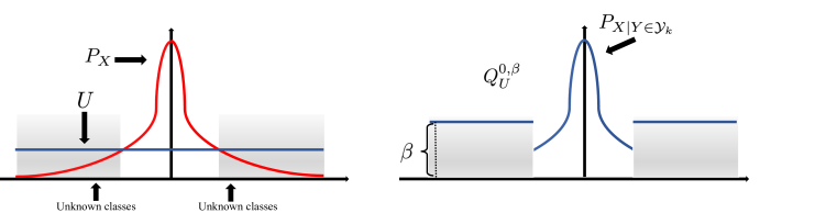
Figure 1: The left figure shows the auxiliary distribution $U$ and marginal distribution $P_{X}$ (red curve: distribution $P_{X}$; blue lines: distribution $U$ introduced in Definition 5; grey regions: the regions for unknown classes). The right figure shows the marginal distribution $Q_{U}^{0,\beta}$ of ideal auxiliary domain generated by $U$, $P_{X|Y\in\mathcal{Y}_{k}}$ and $L_{0,\beta}$ (blue lines and curve: $Q_{U}^{0,\beta}$ defined in Definition 5).

Assumption 1 (Realization for Unknown Classes).

A hypothesis $\mathcal{H}\subset\{{\bm{h}}:\mathcal{X}\rightarrow\mathcal{Y}\}$ is realization for unknown classes, if there exist a hypothesis function $\tilde{\bm{h}}\in\mathcal{H}$ and a distribution $\tilde{P}$ defined over $\mathcal{X}$ with ${\rm supp}~{}\tilde{P}=\mathcal{X}$ satisfying for any ${\bm{h}}\in\mathcal{H}$, there exists ${\bm{h}}^{\prime}\in\mathcal{H}$ such that ${\bm{h}}^{\prime}(\mathbf{x})=\mathbf{y}_{C+1}$, if $\tilde{\bm{h}}(\mathbf{x})=\mathbf{y}_{C+1}$, otherwise, ${\bm{h}}^{\prime}(\mathbf{x})={\bm{h}}(\mathbf{x})$; and

$$\int_{\mathcal{X}\times\mathcal{Y}}\ell(\phi\circ\tilde{\bm{h}}(\mathbf{x}),\phi(\mathbf{y})){\rm d}{P}_{Y|X}(\mathbf{y}|\mathbf{x}){\rm d}\tilde{P}(\mathbf{x})=0,$$

where $\phi$ is a function defined over $\mathcal{Y}$ and defined as follows $\phi(\mathbf{y})=\mathbf{y}_{C+1}$, if $\mathbf{y}=\mathbf{y}_{C+1}$; otherwise, $\phi(\mathbf{y})=\mathbf{y}_{1}$.

Remark 2.

Assumption 1 implies that the hypothesis space $\mathcal{H}$ is complexity enough so that the unknown classes can be classified perfectly by many hypothesis functions. The assumption can be regarded as the open-set version of realization assumption (Shalev-Shwartz & Ben-David, 2014; Mohri et al., 2012). Realization assumption is a basic concept in learning theory.

Theorem 2.

Given a loss $\ell$ satisfying $\ell(\mathbf{y},\mathbf{y}^{\prime})=0$ iff $\mathbf{y}=\mathbf{y}^{\prime}$, and a hypothesis space $\mathcal{H}\subset\{{\bm{h}}:\mathcal{X}\rightarrow\mathbb{R}^{C+1}\}$ satisfying Assumption 1, if $Q_{X,Y}$ is the auxiliary domain for $P_{X,Y}$ and assume $P_{X}\ll Q_{X}\ll\tilde{P}$, where $\tilde{P}$ is the distribution introduced in Assumption 1, then for any $0<\alpha<1$,

$$\begin{split}\min_{{\bm{h}}\in\mathcal{H}}R_{Q}^{\alpha}({\bm{h}})&={\min_{{\bm{h}}\in\mathcal{H}}}R_{P}^{\alpha}({\bm{h}}),\\ \operatorname*{arg\,min}_{{\bm{h}}\in\mathcal{H}}R_{Q}^{\alpha}({\bm{h}})&\subset{\operatorname*{arg\,min}_{{\bm{h}}\in\mathcal{H}}}R_{P}^{\alpha}({\bm{h}}).\end{split}$$

3.3 Construction of Ideal Auxiliary Domain

As mentioned above, the auxiliary domain plays an important role to address the open-set learning problem from a transfer learning perspective. Thus, in this subsection, we first show how to construct an ideal auxiliary domain and then demonstrate how to estimate the ideal auxiliary domain via finite samples. Given an auxiliary distribution $U$ such that $P_{X|Y\in\mathcal{Y}_{k}}\ll U$, we denote $r(\mathbf{x})$ as the density ratio between $P_{X|Y\in\mathcal{Y}_{k}}$ and $U$, i.e., for any $U$-measurable set $A$,

$$P_{X|Y\in\mathcal{Y}_{k}}(A)=\int_{A}r(\mathbf{x}){\rm d}U(\mathbf{x}),$$

and denote ${Q}_{U}^{0,\beta}$ as the marginal distribution defined over $\mathcal{X}$, i.e., for any $U$-measurable set $A$,

$${Q}_{U}^{0,\beta}(A):=\gamma\int_{A}L_{0,\beta}(r(\mathbf{x})){\rm d}U(\mathbf{x}),~{}~{}\textrm{here}$$ (5)

$$\gamma=\frac{1}{1+\beta U(r=0)},$$ (6)

$$L_{0,\beta}(x)=\left\{\begin{aligned} ~{}~{}~{}~{}~{}x+\beta,&~{}~{}~{}~{}~{}~{}~{}x\leq 0,\\ ~{}~{}~{}~{}~{}x,&~{}~{}~{}~{}~{}~{}~{}x>0,\\ \end{aligned}\right.$$

and $\beta>0$ is a parameter to tune the density of ${Q}_{U}^{0,\beta}$ for unknown classes. Then we define the ideal auxiliary domain.

Definition 5 (Ideal Auxiliary Domain (IAD)).

Given the distribution $P_{X,Y}$ defined in Problem 1 and an auxiliary distribution $U$ defined over $\mathcal{X}$ such that $P_{X|Y\in\mathcal{Y}_{k}}\ll U$, then the ideal auxiliary domain regarding to $P_{X,Y}$ is

$${Q}_{U}^{0,\beta}\cdot P_{Y|X},$$

where ${Q}_{U}^{0,\beta}$ is defined in Eq. (5).

In Definition 5, the probability value of distribution $Q_{U}^{0,\beta}$ in space $\mathcal{X}/\ {\rm supp}~{}r$ is a constant $\beta$. In detail, if $P_{X,Y}$ has no overlap between known and unknown classes, any sample from $Q_{X|Y=\mathbf{y}_{C+1}}$ shares same probability (see Figure 1). In addition, an auxiliary distribution $U$ satisfying $P_{X|Y\in\mathcal{Y}_{k}}\ll U$ is needed. The samples drawn from $U$ can be generated by a gaussian distribution or uniform distribution with suitable support set.

Given finite samples $T:=\{\tilde{\mathbf{x}}^{j}\}_{j=1}^{m}$ drawn (i.i.d.) from a given distribution $U$ as introduced in Definition 5. We introduce how to use $T$ and $S$ to construct an approximate form of ${Q}_{U}^{0,\beta}$ introduced in Definition 5.

To simple, we provide a mild assumption as follows.

Assumption 2.

Distributions $P_{X|Y\in\mathcal{Y}_{k}}$ and $U$ introduced in Definition 5 are continuous distributions with density functions $p(\mathbf{x})$ and $q(\mathbf{x})$, respectively.

Remark 3.

The assumption that $P_{X|Y\in\mathcal{Y}_{k}}$ and $U$ are continuous can be replaced by a weaker assumption: $P_{X|Y\in\mathcal{Y}_{k}}$, $U\ll\mu$, where $\mu$ is a measure defined over $\mathcal{X}$. With the weaker assumption, all theorems still hold.

Note that the density ratio $r=p/q$ required in ${Q}_{U}^{0,\beta}$ is unknown. To compute the density ratio $r$ using $S$ and $T$, the density ratio estimation methods are indispensable. Considering the property of statistical convergence, we use kernelized variant of unconstrained least-squares importance fitting (KuLSIF) (Kanamori et al., 2012) to estimate the density ratio in the theoretical part: given RKHS space $\mathcal{H}_{K}$,

$$\min_{w\in\mathcal{H}_{K}}\frac{\sum_{\mathbf{x}\in T}w^{2}(\mathbf{x})}{m}-2\frac{\sum_{(\mathbf{x},\mathbf{y})\in S}w(\mathbf{x})}{n}+\lambda\|w\|_{k}^{2},$$ (7)

where $\lambda$ is the regularization parameter. Then, we assume $\widehat{w}$ is the solution of Eq. (7).

After instance re-weighting, we regard the following measure

$$\widehat{Q}_{T}^{\tau,\beta}:=\frac{\gamma}{m}\sum_{\mathbf{x}\in T}L_{\tau,\beta}({\widehat{w}(\mathbf{x}}))\delta_{\mathbf{x}},~{}~{}~{}$$ (8)

as the approximation of $Q_{U}^{0,\beta}$, where $\gamma$ is defined in Eq. (6),

$$L_{\tau,\beta}(x)=\left\{\begin{aligned} ~{}~{}~{}~{}~{}x+\beta,&~{}~{}~{}~{}~{}~{}~{}x\leq\tau;\\ ~{}~{}~{}~{}~{}x,&~{}~{}~{}~{}~{}~{}~{}2\tau\leq x;\\ ~{}~{}~{}~{}~{}\big{(}1-\frac{\beta}{\tau}\big{)}x+2\beta,&~{}~{}~{}~{}~{}~{}~{}\tau<x<2\tau,\end{aligned}\right.$$

and $\tau>0$ is the threshold to select whether a sample $\mathbf{x}\in T$ is from unknown classes or known classes.

3.4 Empirical Estimation for IAD Risk

In this subsection, we first set the ideal auxiliary domain ${Q}_{U}^{0,\beta}\cdot P_{Y|X}$ as $Q_{X,Y}$, then we analyze the IAD risk $R^{\alpha}_{Q}({\bm{h}})$ from an approximate view, where $\alpha=1-1/\big{(}1+\beta U(r=0)\big{)}$. In detail, the IAD risk $R^{\alpha}_{Q}({\bm{h}})$ can be written as follows

$$R_{Q}^{\alpha}({\bm{h}})=\int_{\mathcal{X}}\ell({\bm{h}}(\mathbf{x}),\mathbf{y}){\rm d}P_{Y|X}(\mathbf{y}|\mathbf{x}){\rm d}{Q}_{U}^{0,\beta}(\mathbf{x}).$$ (9)

Then, we use $\widehat{Q}_{T}^{\tau,\beta}$ (see Eq. (8)) to construct auxiliary risk to approximate the IAD risk.

Definition 6 (Auxiliary Risk).

Given samples $S$ with size $n$ drawn from $P_{X,Y|Y\in\mathcal{Y}_{k}}$ and $T$ with size $m$ drawn from $U$, i.i.d., then the auxiliary risk for a hypothesis function ${\bm{h}}$ is

$$\widehat{R}_{S,T}^{\tau,\beta}({\bm{h}}):=\widehat{R}_{S}({\bm{h}})+\Delta_{S,T}^{\tau,\beta}({\bm{h}}),$$ (10)

where

$$\begin{split}&\widehat{R}_{S}({\bm{h}}):=\frac{1}{n}\sum_{(\mathbf{x},\mathbf{y})\in S}\ell({\bm{h}}({\mathbf{x}}),\mathbf{y}),\\ &\Delta_{S,T}^{\tau,\beta}({\bm{h}}):=\max\{\widehat{R}^{\tau,\beta}_{T}({\bm{h}},\mathbf{y}_{C+1})-\widehat{R}_{S}({\bm{h}},\mathbf{y}_{C+1}),0\},\\ &\widehat{R}^{\tau,\beta}_{T}({\bm{h}},\mathbf{y}_{K+1}):=\frac{1}{\gamma}\int_{\mathcal{X}}\ell({\bm{h}}(\mathbf{x}),\mathbf{y}_{C+1}){\rm d}\widehat{Q}_{T}^{\tau,\beta}(\mathbf{x})\\ &~{}~{}~{}~{}~{}~{}~{}~{}~{}~{}~{}~{}~{}~{}~{}~{}~{}~{}~{}~{}~{}~{}~{}~{}~{}~{}=\frac{1}{m}\sum_{\mathbf{x}\in T}L_{\tau,\beta}({\widehat{w}(\mathbf{x}}))\ell({\bm{h}}({\mathbf{x}}),\mathbf{y}_{C+1}),\\ &\widehat{R}_{S}({\bm{h}},\mathbf{y}_{C+1}):=\frac{1}{n}\sum_{(\mathbf{x},\mathbf{y})\in S}\ell({\bm{h}}({\mathbf{x}}),\mathbf{y}_{C+1}),\end{split}$$

here $\widehat{Q}_{T}^{\tau,\beta}$ is defined in Eq. (8) and $\gamma$ is defined in Eq. (6).

Theorem 3 implies that $(1-\alpha)\widehat{R}_{S,T}^{\tau,\beta}({\bm{h}})$ can approximate $R^{\alpha}_{Q}({\bm{h}})$ uniformly.

Theorem 3.

Assume assumption 2 holds, the feature space $\mathcal{X}$ is compact and the hypothesis space $\mathcal{H}\subset\{{\bm{h}}:\mathcal{X}\rightarrow\mathbb{R}^{C+1}\}$ has finite Natarajan dimension (Shalev-Shwartz & Ben-David, 2014). Let the RKHS $\mathcal{H}_{K}$ be the Hilbert space with gaussian kernel. Suppose that loss function is bounded by $c$, the density $r\in\mathcal{H}_{K}$ and set the regularization parameter $\lambda=\lambda_{n,m}$ in KuLSIF (see Eq. (7)) such that

$$\lim_{n,m\rightarrow 0}\lambda_{n,m}=0,~{}~{}~{}\lambda_{n,m}^{-1}=O({\min\{n,m\}}^{1-\delta}),$$

where $0<\delta<1$ is any constant, then for any $0\leq\alpha<1$,

$$\begin{split}&\sup_{{\bm{h}}\in\mathcal{H}}|(1-\alpha)\widehat{R}_{S,T}^{\tau,\beta}({\bm{h}})-R^{\alpha}_{Q}({\bm{h}})|\\ \leq&c\big{(}\max\{1,\frac{\beta}{\tau}\}+\beta\big{)}O_{p}(\lambda^{\frac{1}{2}}_{n,m})+\gamma c\beta U(0<r\leq 2\tau),\end{split}$$

where $O_{p}$ denotes the probabilistic order, $\gamma=1-\alpha,\beta=\frac{\alpha}{\gamma U(r=0)}$, $\widehat{R}_{S,T}^{\tau,\beta}({\bm{h}})$ is defined in Eq. (10), and $R^{\alpha}_{Q}({\bm{h}})$ is the IAD risk defined in Eq. (9).

Note that $U(0<r\leq 2\tau)\rightarrow 0$, if $\tau\rightarrow 0$, and Theorem 3 has indicated that if we omit the term $(1-\alpha)c\beta U(0<p/q\leq 2\tau)$ and set $m\geq n$, the gap between $(1-\alpha)\widehat{R}_{S,T}^{\tau,\beta}({\bm{h}})$ and $R^{\alpha}_{Q}({\bm{h}})$ is close to $O_{p}(1/\sqrt{n})$ by choosing a small $\delta$.

3.5 Main Theoretical Results

In this subsection, we analyze the relationship between $R^{\alpha}_{P}({\bm{h}})$ and $\widehat{R}_{S,T}^{\tau,\beta}({\bm{h}})$ based on Theorems 1, 2 and 3.

Theorem 4 (Uniform Bound Based on Transfer Learning).

Given the same conditions and assumptions in Theorems 1 and 3, then for any $0\leq\alpha<1$, ${\bm{h}}\in\mathcal{H}$,

$$\begin{split}&|(1-\alpha)\widehat{R}_{S,T}^{\tau,\beta}({\bm{h}})-R^{\alpha}_{P}({\bm{h}})|\\ \leq&c\big{(}\max\{1,\frac{\beta}{\tau}\}+\beta\big{)}O_{p}(\lambda^{\frac{1}{2}}_{n,m})+\gamma c\beta U(0<r\leq 2\tau)\\ +&\alpha d^{\ell}_{{\bm{h}},\mathcal{H}}(P_{X|Y=\mathbf{y}_{C+1}},Q_{X|Y=\mathbf{y}_{C+1}})+\alpha\Lambda,\end{split}$$

where $\lambda_{n,m}$ is defined in Theorem 3, $\gamma=1-\alpha,\beta=\frac{\alpha}{\gamma U(r=0)}$, $\widehat{R}_{S,T}^{\tau,\beta}({\bm{h}})$ is defined in Eq. (10), $d^{\ell}_{{\bm{h}},\mathcal{H}}$ is the disparity discrepancy defined in Definition 4, $\Lambda$ is the combined risk defined in Eq. (4) and $O_{p}$ is the probabilistic order (independent of $c,\beta,\tau$ and $\alpha$).

Theorem 4 indicates that the gap between $(1-\alpha)\widehat{R}_{S,T}^{\tau,\beta}({\bm{h}})$ and $R^{\alpha}_{P}({\bm{h}})$ is controlled by four special terms. The combined risk $\Lambda$ and domain discrepancy for unknown classes can be regarded as constants. The other two terms could be small enough, if $n,m\rightarrow+\infty$ and $\tau$ is a small value.

Theorem 5 (Estimation Error for OSL).

Given the same conditions and assumptions in Theorems 2 and 3, for any $0\leq\alpha<1$, if we assume $\widehat{\bm{h}}\in\operatorname*{arg\,min}_{{\bm{h}}\in\mathcal{H}}\widehat{R}_{S,T}^{\tau,\beta}({\bm{h}}),$ then $|R_{P}^{\alpha}(\widehat{\bm{h}})-\min_{{\bm{h}}\in\mathcal{H}}R^{\alpha}_{P}({\bm{h}})|$ has an upper bound

$$\begin{split}&c\big{(}\max\{1,\frac{\beta}{\tau}\}+\beta\big{)}O_{p}(\lambda^{\frac{1}{2}}_{n,m})+4\gamma c\beta U(0<r\leq 2\tau),\end{split}$$

where $\lambda_{n,m}$ is defined in Theorem 3, $\gamma=1-\alpha,\beta=\frac{\alpha}{\gamma U(r=0)}$, $\widehat{R}_{S,T}^{\tau,\beta}({\bm{h}})$ is defined in Eq. (10) and $O_{p}$ is the probabilistic order (independent of $c,\beta,\tau$ and $\alpha$).

If we select a small $\tau$ to make $U(0<r\leq 2\tau)$ small enough and set $m\geq n$, then under some assumptions, the following optimization problem

$$\min_{{\bm{h}}\in\mathcal{H}}\widehat{R}_{S,T}^{\tau,\beta}({\bm{h}})$$ (11)

is almost classifier-consistent with estimation error close to $O_{p}(1/\sqrt{n})$. Additionally, the weight estimation in Theorem 5 is crucial. To weaken the effect of weight estimation in area ${\rm supp}~{}P_{X|Y\in\mathcal{Y}_{k}}$, we introduce a proxy for $\widehat{R}_{S,T}^{\tau,\beta}({\bm{h}})$.

Definition 7 (Proxy of Auxiliary Risk).

Given samples $S$ with size $n$ drawn from $P_{X,Y|Y\in\mathcal{Y}_{k}}$ and $T$ with size $m$ drawn from $U$, i.i.d., then the auxiliary risk for a hypothesis function ${\bm{h}}$ is

$$\widetilde{R}_{S,T}^{\tau,\beta}({\bm{h}}):=\widehat{R}_{S}({\bm{h}})+\frac{\alpha\gamma^{\prime}}{1-\alpha}\widehat{R}_{S,T,u}^{\tau,\beta}({\bm{h}}),$$ (12)

where $\gamma^{\prime}=1/U(r=0)$, $\widehat{R}_{S}({\bm{h}})$ is defined in Definition 6,

$$\begin{split}\widehat{R}_{S,T,u}^{\tau,\beta}({\bm{h}}):=\frac{1}{m}\sum_{\mathbf{x}\in T}L_{\tau,\beta}^{-}({\widehat{w}(\mathbf{x}}))\ell({\bm{h}({\mathbf{x}})},\mathbf{y}_{C+1}),\end{split}$$

here

$$L_{\tau,\beta}^{-}(x)=\left\{\begin{aligned} x+\beta,&~{}~{}~{}~{}x\leq\tau;\\ 0,&~{}~{}~{}~{}2\tau\leq x;\\ -\frac{\tau+\beta}{\tau}x+2\tau+2\beta,&~{}~{}~{}~{}\tau<x<2\tau.\end{aligned}\right.$$

Then, a result similar to Theorem 5 for auxiliary risk $\widetilde{R}_{S,T}^{\tau,\beta}$ is given as follows.

Theorem 6 (Estimation Error for OSL).

Given the same conditions and assumptions in Theorem 5, for any $0\leq\alpha<1$, if we assume $\widetilde{\bm{h}}\in\operatorname*{arg\,min}_{{\bm{h}}\in\mathcal{H}}\widetilde{R}_{S,T}^{\tau,\beta}({\bm{h}})$, then $|R_{P}^{\alpha}(\widetilde{\bm{h}})-\min_{{\bm{h}}\in\mathcal{H}}R^{\alpha}_{P}({\bm{h}})|$ has an upper bound

$$\begin{split}&c\gamma^{\prime}\big{(}1+\tau+\frac{\beta}{\tau}+\beta\big{)}O_{p}(\lambda^{\frac{1}{2}}_{n,m})+4c\gamma^{\prime}\alpha\beta U(0<r\leq 2\tau),\end{split}$$

where $\lambda_{n,m}$, $\beta$ are introduced in Theorem 5, $\gamma^{\prime}$ and $\widetilde{R}_{S,T}^{\tau,\beta}({\bm{h}})$ are defined in Definition 7, and $O_{p}$ is the probabilistic order (independent of $c,\beta,\tau,\gamma^{\prime}$ and $\alpha$).

4 A Principle Guided OSL Algorithm

Inspired by Theorem 6, we focus on the following problem

$$\min_{{\bm{\Theta}}}\big{(}\widehat{R}_{S}({\bm{h}}_{\bm{\Theta}})+\mu\widehat{R}_{S,T,u}^{\tau,\beta}({\bm{h}}_{\bm{\Theta}})\big{)},$$ (13)

where $\mu$ is a positive parameter, $\widehat{R}_{S,T,u}^{\tau,\beta}({\bm{h}})$ is defined in Eq. (12), ${\bm{h}}_{\bm{\Theta}}$ is a hypothesis function based on a neural network, and ${\bm{\Theta}}$ is parameters of the neural network. To optimize ${\bm{h}}_{\bm{\Theta}}$ to solve the minimization problem defined in Eq. (13), we have the following five steps.

Step 1 (Feature Encoding). Train the samples $S$ to get a closed-set classifier ${\bm{h}}_{{\bm{\Theta}}_{0}}$, and designate the output of second to the last layer (without softmax) ${\bm{l}}$ of ${\bm{h}}_{{\bm{\Theta}}_{0}}$ as the encoded feature vector, i.e., $X_{\textrm{encoder}}={\bm{l}}(X)$. The new encoded feature space is denoted as $\mathcal{X}_{\textrm{encoder}}$.

Step 2 (Initialize the Auxiliary Domain). Randomly generate samples $T$ from space $\mathcal{X}_{\textrm{encoder}}$. By default, we generate $T$ by uniform distribution and set the size $m$ is $3n$. We update the samples $S=\{({\bm{l}}(\mathbf{x}),\mathbf{y}):(\mathbf{x},\mathbf{y})\in S\}$.

Step 3 (Construct the Auxiliary Domain). Estimate the weights $\widehat{w}$ with samples $S$ and $T$ as the input. The higher the weight is, the more likely a generated sample belongs to the known classes. The parameters selection details are shown as follows.

Weight estimation algorithm: In the theoretical part, KuLSIF is selected to estimate weights. Kernel mean matching (KMM) (Gretton et al., 2012) is also an alternative solution (Cortes et al., 2008). However, in practice, KuLSIF and KMM have time complexity $O((m+n)^{2})$ (Kanamori et al., 2012), which is not suitable for large datasets. The kernel bandwidth selection also impacts the overall performance (Liu et al., 2020). Thus, we recommend using the outlier sample score (with range $[0,1]$) given by isolation forest (iForest) (Liu et al., 2008) as the sample weights, which has time complexity ${O}((n+m)\log(n+m))$. Close to $1$ means known classes while close to $0$ means unknown classes.

The $\tau$ is a threshold to split the generated samples $T$ into known and unknown samples. Considering we are using iForest, based on the predicted sample score $[s_{1},...,s_{m}]$ (descending order), we set $\tau=s_{[t*m]}$, where $t\in(0,1)$ is the proportion that the generated samples selected as unknown samples. We set $t=10\%$ as default.

The $\beta$ and $\mu$ control jointly the importance of correctly classified unknown samples. We set $\mu$ as a dynamical parameter depending on $\beta$: $\mu=\frac{n\beta}{n^{\prime}+0.0001}$, where $n^{\prime}$ is number of samples in training samples actually predicted as unknown. For example, if $\beta=0.05$, $n$ is $1000$, there are $10$ samples in training samples are predicted as unknown, then $\mu\approx 5$.

Step 4 ($\mathbf{Softmax}_{C+1}$). Initialize an open-set learning neural network with samples $S$ and $T$ as the input and $C+1$ Softmax (Qin et al., 2019) nodes as the output.

Step 5 (Open-set Learning). Train the $\mathbf{Softmax}_{C+1}$ neural network with the cost function defined in Eq. (13) with both $S$ and $T$.

5 Experiments and Results

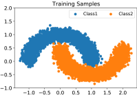
(a) Double-moon dataset

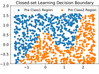
(b) Closed-set classification

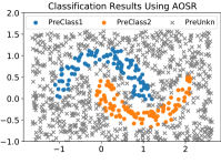
(c) Open-set classification

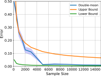
(d) Error and Sample Size

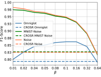
(e) Parameter Analysis for $\beta$

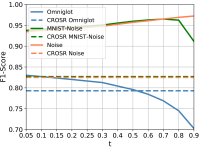
(f) Parameter Analysis for $t$

Figure 2: (a) is the training samples for double-moon dataset. (b) is the decision regions under closed-set learning setting for double-moon dataset. (c) is the decision regions under open-set learning setting for double-moon dataset. (d) is the relationship between error and sample size. (e) is the parameter analysis for $\beta$. (f) is the parameter analysis for $t$.

First, we implement AOSR on toy dataset with different sample size to reveal the relationship between sample size $n$ and error ($O(1/\sqrt{n})$). Then, we evaluate the efficacy of AOSR on benchmark datasets.

5.1 Datasets

In this paper, we verify the efficacy of algorithm AOSR on double-moon dataset and several real world datasets:

$\bullet$ Double-moon dataset (toy). The double-moon dataset consists of two different clusters. Samples from different clusters are regarded as known samples with different label. Samples from other region are regarded as unknown samples drawn from uniform distribution, i.i.d. The ratio between the sizes of known and unknown samples is $1$.

$\bullet$ Following the set up in Yoshihashi et al. (2019), we use MNIST (LeCun & Cortes, 2010) as the training samples and use Omniglot (Ager, 2008), MNIST-Noise, and Noise (Liu et al., 2021) datasets as unknown classes. Omniglot contains alphabet characters. Noise is synthesized by sampling each pixel value from a uniform distribution on $[0,1]$. MNIST-Noise is synthesized by adding noise on MNIST test samples. Each dataset has $10,000$ test samples.

$\bullet$ Following Yoshihashi et al. (2019), we use CIFAR-$10$ (Krizhevsky & Hinton, 2009) as training samples and collect unknown samples from ImageNet and LSUN. We resized/cropped them so that they would be the same size as the known samples. Hence, we generate four datasets ImageNet-crop, ImageNet-resize, LSUN-crop and LSUN-resize as unknown classes. Each dataset contains $10,000$ test samples.

$\bullet$ Following Yoshihashi et al. (2019), Chen et al. (2021), Sun et al. (2020), we use MNIST (LeCun & Cortes, 2010), SVHN (Netzer et al., 2011) and CIFAR-$10$ (Krizhevsky & Hinton, 2009) to construct different OSL tasks. For MNIST, SVHN and CIFAR-$10$, each dataset is randomly divided into $6$ known classes and $4$ unknown classes. In addition, we construct CIFAR+$10$ and CIFAR+$50$ by randomly selection $6$ known classes and $10$ or $50$ unknown classes from CIFAR-$100$ (Krizhevsky & Hinton, 2009).

5.2 Open-set Learning Demonstration

Table 1: The performance on dataset CIFAR-$10$ is evaluated by macro-averaged F1 scores in 11 classes ($10$ known classes and $1$ unknown class). We report the experimental results reproduced by Yoshihashi et al. (2019). A larger score is better.

Algorithm	ImageNet-crop	ImageNet-resize	LSUN-crop	LSUN-resize
Softmax	0.639	0.653	0.642	0.647
Openmax (Bendale & Boult, 2016)	0.660	0.684	0.657	0.668
Counterfactual (Neal et al., 2018)	0.636	0.635	0.650	0.648
CROSR (Yoshihashi et al., 2019)	0.721	0.735	0.720	0.749
C2AE (Oza & Patel, 2019)	0.837	0.826	0.783	0.801
CGDL (Sun et al., 2020)	0.840	0.832	0.806	0.812
Ours (AOSR)	0.798	0.795	0.839	0.838

Table 2: The performance on dataset MNIST is evaluated by macro-averaged F1 scores in 11 classes.

Algorithm	Omniglot	MNIST-Noise	Noise
Softmax	0.595	0.801	0.829
Openmax	0.780	0.816	0.826
CROSR	0.793	0.827	0.826
CGDL	0.850	0.887	0.859
Ours (AOSR)	0.825	0.953	0.953

Table 3: The performance on MNIST, SVHN, CIFAR-$10$, CIFAR+$10$ and CIFAR+$50$ are evaluated by macro-averaged F1 scores. We report the experimental results reported by Sun et al. (2020).

Algorithm	MNIST	SVHN	CIFAR-$10$	CIFAR+$10$	CIFAR+$50$
Softmax	0.768	0.725	0.600	0.701	0.637
Openmax (Bendale & Boult, 2016)	0.798	0.737	0.623	0.731	0.676
CROSR (Yoshihashi et al., 2019)	0.803	0.753	0.668	0.769	0.684
GDFR (Perera et al., 2020)	0.821	0.716	0.700	0.776	0.683
CGDL (Sun et al., 2020)	0.837	0.776	0.655	0.760	0.695
Ours (AOSR)	0.850	0.842	0.705	0.773	0.706

Here we break down the entire learning process and demonstrate the inter-media process of each step on the toy dataset. This experiment is aiming to provide an visualization aid on understanding the open-set learning process.

To start with, we plot the double-moon dataset in Figure 2 (a). The objective of closed-set learning is to build a classifier that can split the samples with different labels. To achieve this goal, we build a simple neural network with sparse categorical cross-entropy as the loss function.

The closed-set learning result is shown in Figure 2 (b). In this case, the closed-set classifier splits the samples with different labels well. However, the closed-set classifier does not consider the boundary of support set for training domain, that is, any new samples that does not located in the support set, the closed-set classifier still gives a known label.

Figure 2 (c) is the open-set learning result. To recognize the unknown samples, the open-set classifier should delineate a boundary between the known and unknown classes. To achieve this goal, we use $\mathbf{Softmax}_{C+1}$ as the final output and Eq. (13) as the cost function. The AOSR will push the neural network to give label $\mathbf{y}_{C+1}$ on unknown samples.

5.3 Experimental Setup

$\bullet$ AOSR has several hyper-parameters: $\beta$, $t$, $\mu$ and $m$. For all tasks, we set $m=3n,~{}t=10\%$ as default. $\mu$ is a dynamic parameter depending on $\beta$. $\beta$ is selected from $0.01$ to $2.5$. Details on the selection of parameters are available at github.com/Anjin-Liu/Openset_Learning_AOSR.

$\bullet$ For datasets MNIST, Omnilot, MNIST-Noise, Noise, we use the same setting of Yoshihashi et al. (2019) and Sun et al. (2020) to extract the features. Same as Yoshihashi et al. (2019), DHRNet-$92$ is used as the backbone for CIFAR-$10$, ImageNet and LSUN datasets. For different tasks MNIST, SVHN, CIFAR-$10$, CIFAR+$10$ and CIFAR+$50$, the backbone is the re-designed VGGNet used by Yoshihashi et al. (2019) and Sun et al. (2020).

$\bullet$ We select baseline algorithms as follows: SoftMax, OpenMax (Bendale & Boult, 2016), Counterfactual (Neal et al., 2018), CROSR (Yoshihashi et al., 2019), C2AE (Oza & Patel, 2019), and CGDL (Sun et al., 2020).

5.4 Evaluation

Following Yoshihashi et al. (2019), the macro-average F1 scores are used to evaluate OSL. The area under the receiver operating characteristic (AUROC) (Neal et al., 2018) is also frequently used (Neal et al., 2018; Chen et al., 2020). Note that AUROC used in (Neal et al., 2018; Chen et al., 2020) is suitable for global threshold-based OSL algorithms that recognize unknown samples by a fix threshold (Neal et al., 2018). However, AOSR recognizes unknown samples based on the score of hypothesis function, thus, AOSR uses different thresholds for different samples. This implies that AUROC used in (Neal et al., 2018; Chen et al., 2020) may be not suitable for our algorithm. In this paper, we use macro-average F1 scores to evaluate our algorithm.

5.5 Experimental Evaluation and Result Analysis

Experiment results on double-moon dataset are summarized in Figure 2 (d). We implement double-moon dataset with varying size $n$ . We also generate $n$ test samples. For a different sample size, we run $100$ times and report the mean accuracy and standard error in Figure 2 (d). Based on Figure 2 (d), the accuracy increases as the increase of training sample size $n$ increases. When $n\rightarrow 15,000$, the accuracy approximates at $100\%$. In particular, the green curve $0.5/\sqrt{n}$ and the yellow curve $8/\sqrt{n}$ jointly control the curve of accuracy, implying the error of AOSR is controlled by $O(1/\sqrt{n})$.

Table 4: Ablation study on dataset MNIST, Omnilot, MNIST-Noise and Noise.

Tasks	Only iForest	$\beta$=0	$\mu$=0	w/KMM	w/KuLSIF	AOSR
Avg	0.680	0.677	0.677	0.907	0.855	0.910

Experiment results on real datasets are summarized in Tables 1, 2 and 3. For all tasks, we run AOSR $5$ times and report the mean results by using F1 score (Powers, 2020). In general, AOSR shows the promising performance when compared to baseline algorithms. The effectiveness of AOSR indicates that our theory is effective and practical.

Parameter analysis for $\beta$ and $t$ is given in Figure 2 (e), (f). We run AOSR with varying values of $\beta,t$ on MNIST tasks. From Figure 2 (e), we observe that 1) when $\beta$ increases from $0.01$ to $0.64$, the F1 scores for Noise and MNIST-Noise decrease; 2) as increasing $\beta$ from $0.01$ to $0.16$, the F1 score for Omniglot increases. When $\beta>1.6$, the performance for Omniglot dramatically dropped to baseline. Additionally, according to Figure 2 (f), we find that by changing $t$ in the range of $[0.05,0.30]$, AOSR achieve stable performance.

Ablation study on datasets MNIST, Omnilot, MNIST-Noise and Noise is shown in Table 4. By adjusting different components of AOSR, Table 4 indicates that each component of AOSR is important and necessary. Note that if we replace iForest by KMM in AOSR, the performance ($0.907$) is close to AOSR ($0.910$). This implies that KMM may be a good choice, if we omit the time complexity of KMM.

6 Discussion

Relation with Generative Models. Algorithms based on generative models are the mainstream for OSL. CGDL (Sun et al., 2020), C2AE (Oza & Patel, 2019) and Counterfactual (Neal et al., 2018) are the representative works based on generative models. AOSR can be regarded as the weight-based generative model, but is very different from the mainstream generative model-based algorithms (feature map-based generative model (Sun et al., 2020; Oza & Patel, 2019; Neal et al., 2018)). Form the theoretical perspective, it is necessary to develop theory to guarantee the generalization ability of feature map-based generative models. Here we propose an interesting and important problem: how to develop generalization theory for feature map-based generative models under open-set assumption ?

Relation with PU Learning. Positive-unlabeled learning (PU learning) (Niu et al., 2016) is a special binary classification task, which assumes only unlabeled samples and positive samples (i.e., samples with positive labels) are available. Our theory is deeply related to PU learning. If we regard the known samples $S$ and the auxiliary samples as the positive samples and the unlabeled samples, respectively. Then, our theory degenerates into the PU learning theory.

Remaining Problems in OSL Theory. We list several interesting and important problems for OSL theory as follows. 1. How to construct weaker assumption to replace assumption 1 for achieving similar results ?
2. Without assumption 1, what will happen ?
3. Is it possible for OSL to achieve agnostic PAC learnability and achieve fast learning rate $O_{p}(1/{n}^{a})$, for $a>0.5$ ?
4. Is it possible to construct OSL learning theory by stability theory (Bousquet & Elisseeff, 2002) ?

7 Conclusion and Future Work

This paper mainly focuses on the learning theory for open-set learning. The generalization error bounds proved in our work provide the first almost-PAC-style guarantee on open-set learning. Based on our theory, a principle guided algorithm AOSR is proposed. Experiments on real datasets indicate that AOSR achieves competitive performance when compared with baselines. In future, we will focus on developing more powerful OSL algorithms based on our theory and dynamic weight technique (Fang et al., 2020a). With the dynamic weight , we can update the weight for each epoch and make a better integration between instance-weighting and deep learning.

References

- Ager (2008) Ager, S. Omniglot-writing systems and languages of the world. Retrieved January, 27:2008, 2008.
- Ben-David et al. (2006) Ben-David, S., Blitzer, J., Crammer, K., and Pereira, F. Analysis of representations for domain adaptation. In NeurIPS, pp. 137–144, 2006.
- Bendale & Boult (2016) Bendale, A. and Boult, T. E. Towards open set deep networks. In CVPR, pp. 1563–1572. IEEE Computer Society, 2016.
- Boult et al. (2019) Boult, T. E., Cruz, S., Dhamija, A. R., Günther, M., Henrydoss, J., and Scheirer, W. J. Learning and the unknown: Surveying steps toward open world recognition. In AAAI, pp. 9801–9807, 2019.
- Bousquet & Elisseeff (2002) Bousquet, O. and Elisseeff, A. Stability and generalization. J. Mach. Learn. Res., 2:499–526, 2002.
- Busto et al. (2020) Busto, P. P., Iqbal, A., and Gall, J. Open set domain adaptation for image and action recognition. IEEE Trans. Pattern Anal. Mach. Intell., pp. 413–429, 2020.
- Chen et al. (2020) Chen, G., Qiao, L., Shi, Y., Peng, P., Li, J., Huang, T., Pu, S., and Tian, Y. Learning open set network with discriminative reciprocal points. In ECCV, volume 12348, pp. 507–522. Springer, 2020.
- Chen et al. (2021) Chen, G., Peng, P., Wang, X., and Tian, Y. Adversarial reciprocal points learning for open set recognition. CoRR, abs/2103.00953, 2021.
- Collobert & Weston (2008) Collobert, R. and Weston, J. A unified architecture for natural language processing: deep neural networks with multitask learning. In ICML, volume 307, pp. 160–167, 2008.
- Cortes et al. (2008) Cortes, C., Mohri, M., Riley, M., and Rostamizadeh, A. Sample selection bias correction theory. In ALT, volume 5254, pp. 38–53. Springer, 2008.
- de O. Cardoso et al. (2017) de O. Cardoso, D., Gama, J., and França, F. M. G. Weightless neural networks for open set recognition. Mach. Learn., pp. 1547–1567, 2017.
- Dhamija et al. (2018) Dhamija, A. R., Günther, M., and Boult, T. E. Reducing network agnostophobia. In NeurIPS, pp. 9175–9186, 2018.
- Dong et al. (2019) Dong, J., Cong, Y., Sun, G., and Hou, D. Semantic-transferable weakly-supervised endoscopic lesions segmentation. In ICCV, pp. 10711–10720. IEEE, 2019.
- Dong et al. (2020a) Dong, J., Cong, Y., Sun, G., Liu, Y., and Xu, X. CSCL: critical semantic-consistent learning for unsupervised domain adaptation. In ECCV, volume 12353 of Lecture Notes in Computer Science, pp. 745–762. Springer, 2020a.
- Dong et al. (2020b) Dong, J., Cong, Y., Sun, G., Zhong, B., and Xu, X. What can be transferred: Unsupervised domain adaptation for endoscopic lesions segmentation. In CVPR, pp. 4022–4031. IEEE, 2020b.
- Dong et al. (2021) Dong, J., Cong, Y., Sun, G., Yang, Y., Xu, X., and Ding, Z. Weakly-supervised cross-domain adaptation for endoscopic lesions segmentation. IEEE Trans. Circuits Syst. Video Technol., 31(5):2020–2033, 2021.
- Fang et al. (2020a) Fang, T., Lu, N., Niu, G., and Sugiyama, M. Rethinking importance weighting for deep learning under distribution shift. In NeurIPS, 2020a.
- Fang et al. (2020b) Fang, Z., Lu, J., Liu, F., Xuan, J., and Zhang, G. Open set domain adaptation: Theoretical bound and algorithm. IEEE Transactions on Neural Networks and Learning Systems, 2020b.
- Ge et al. (2017) Ge, Z., Demyanov, S., and Garnavi, R. Generative openmax for multi-class open set classification. In BMVC, 2017.
- Geng et al. (2018) Geng, C., Huang, S., and Chen, S. Recent advances in open set recognition: A survey. CoRR, abs/1811.08581, 2018.
- Graves & Jaitly (2014) Graves, A. and Jaitly, N. Towards end-to-end speech recognition with recurrent neural networks. In ICML, pp. 1764–1772. JMLR.org, 2014.
- Gretton et al. (2012) Gretton, A., Borgwardt, K. M., Rasch, M. J., Schölkopf, B., and Smola, A. J. A kernel two-sample test. J. Mach. Learn. Res., pp. 723–773, 2012.
- Jain et al. (2014) Jain, L. P., Scheirer, W. J., and Boult, T. E. Multi-class open set recognition using probability of inclusion. In ECCV, pp. 393–409, 2014.
- Kanamori et al. (2012) Kanamori, T., Suzuki, T., and Sugiyama, M. Statistical analysis of kernel-based least-squares density-ratio estimation. Mach. Learn., pp. 335–367, 2012.
- Krizhevsky & Hinton (2009) Krizhevsky, A. and Hinton, G. Convolutional deep belief networks on cifar-10. Technical report, Citeseer, 2009.
- LeCun & Cortes (2010) LeCun, Y. and Cortes, C. MNIST handwritten digit database. 2010.
- Liu et al. (2019) Liu, F., Lu, J., Han, B., Niu, G., Zhang, G., and Sugiyama, M. Butterfly: A panacea for all difficulties in wildly unsupervised domain adaptation. In NeurIPS LTS Workshop, 2019.
- Liu et al. (2020) Liu, F., Xu, W., Lu, J., Zhang, G., Gretton, A., and Sutherland, D. J. Learning deep kernels for non-parametric two-sample tests. In ICML, 2020.
- Liu et al. (2008) Liu, F. T., Ting, K. M., and Zhou, Z.-H. Isolation forest. In 2008 eighth ieee international conference on data mining, pp. 413–422. IEEE, 2008.
- Liu et al. (2018) Liu, S., Garrepalli, R., Dietterich, T. G., Fern, A., and Hendrycks, D. Open category detection with PAC guarantees. ICML, 2018.
- Liu et al. (2021) Liu, Y., Qin, Z., Anwar, S., Ji, P., Kim, D., Caldwell, S., and Gedeon, T. Invertible denoising network: A light solution for real noise removal. CVPR, 2021.
- Lu et al. (2015) Lu, J., Behbood, V., Hao, P., Zuo, H., Xue, S., and Zhang, G. Transfer learning using computational intelligence: A survey. Knowl. Based Syst., 80:14–23, 2015.
- Luo et al. (2020a) Luo, Y., Huang, Z., Wang, Z., Zhang, Z., and Baktashmotlagh, M. Adversarial bipartite graph learning for video domain adaptation. In ICMM, pp. 19–27, 2020a.
- Luo et al. (2020b) Luo, Y., Wang, Z., Huang, Z., and Baktashmotlagh, M. Progressive graph learning for open-set domain adaptation. In ICML, volume 119 of Proceedings of Machine Learning Research, pp. 6468–6478. PMLR, 2020b.
- Mansour et al. (2009) Mansour, Y., Mohri, M., and Rostamizadeh, A. Domain adaptation: Learning bounds and algorithms. In COLT, 2009.
- Mohri et al. (2012) Mohri, M., Rostamizadeh, A., and Talwalkar, A. Foundations of Machine Learning. 2012.
- Neal et al. (2018) Neal, L., Olson, M. L., Fern, X. Z., Wong, W., and Li, F. Open set learning with counterfactual images. In ECCV, pp. 620–635. Springer, 2018.
- Netzer et al. (2011) Netzer, Y., Wang, T., Coates, A., Bissacco, A., Wu, B., and Ng, A. Y. Reading digits in natural images with unsupervised feature learning. 2011.
- Niu et al. (2016) Niu, G., du Plessis, M. C., Sakai, T., Ma, Y., and Sugiyama, M. Theoretical comparisons of positive-unlabeled learning against positive-negative learning. In NeurIPS, pp. 1199–1207, 2016.
- Niu et al. (2020) Niu, S., Liu, Y., Wang, J., and Song, H. A decade survey of transfer learning (2010-2020). IEEE Trans. Artif. Intell., 1(2):151–166, 2020.
- Oza & Patel (2019) Oza, P. and Patel, V. M. C2AE: class conditioned auto-encoder for open-set recognition. In CVPR, pp. 2307–2316. Computer Vision Foundation / IEEE, 2019.
- Pan & Yang (2010) Pan, S. J. and Yang, Q. A survey on transfer learning. IEEE Trans. Knowl. Data Eng., 22(10):1345–1359, 2010.
- Perera et al. (2020) Perera, P., Morariu, V. I., Jain, R., Manjunatha, V., Wigington, C., Ordonez, V., and Patel, V. M. Generative-discriminative feature representations for open-set recognition. In CVPR, pp. 11811–11820. IEEE, 2020.
- Powers (2020) Powers, D. M. Evaluation: from precision, recall and f-measure to roc, informedness, markedness and correlation. arXiv preprint arXiv:2010.16061, 2020.
- Qin et al. (2019) Qin, Z., Kim, D., and Gedeon, T. Rethinking softmax with cross-entropy: Neural network classifier as mutual information estimator. arXiv preprint arXiv:1911.10688, 2019.
- Rudd et al. (2018) Rudd, E. M., Jain, L. P., Scheirer, W. J., and Boult, T. E. The extreme value machine. IEEE Trans. Pattern Anal. Mach. Intell., pp. 762–768, 2018.
- Santurkar et al. (2018) Santurkar, S., Schmidt, L., and Madry, A. A classification-based study of covariate shift in GAN distributions. In ICML, volume 80, pp. 4487–4496. PMLR, 2018.
- Scheirer et al. (2013) Scheirer, W. J., de Rezende Rocha, A., Sapkota, A., and Boult, T. E. Toward open set recognition. IEEE Trans. Pattern Anal. Mach. Intell., pp. 1757–1772, 2013.
- Scheirer et al. (2014) Scheirer, W. J., Jain, L. P., and Boult, T. E. Probability models for open set recognition. IEEE Trans. Pattern Anal. Mach. Intell., pp. 2317–2324, 2014.
- Shalev-Shwartz & Ben-David (2014) Shalev-Shwartz, S. and Ben-David, S. Understanding machine learning: From theory to algorithms. In Cambridge university press, 2014.
- Simonyan & Zisserman (2015) Simonyan, K. and Zisserman, A. Very deep convolutional networks for large-scale image recognition. In ICLR, 2015.
- Sun et al. (2020) Sun, X., Yang, Z., Zhang, C., Peng, G., and Ling, K. V. Conditional gaussian distribution learning for open set recognition. CVPR, abs/2003.08823, 2020.
- Wang et al. (2020) Wang, Z., Luo, Y., Huang, Z., and Baktashmotlagh, M. Prototype-matching graph network for heterogeneous domain adaptation. In ICMM, pp. 2104–2112, 2020.
- Yang et al. (2020) Yang, H.-M., Zhang, X.-Y., Yin, F., Yang, Q., and Liu, C.-L. Convolutional prototype network for open set recognition. IEEE Transactions on Pattern Analysis and Machine Intelligence, 2020.
- Yoshihashi et al. (2019) Yoshihashi, R., Shao, W., Kawakami, R., You, S., Iida, M., and Naemura, T. Classification-reconstruction learning for open-set recognition. In CVPR, pp. 4016–4025, 2019.
- Zhang et al. (2019) Zhang, Y., Liu, T., Long, M., and Jordan, M. I. Bridging theory and algorithm for domain adaptation. In ICML, volume 97, pp. 7404–7413. PMLR, 2019.
- Zhong et al. (2020) Zhong, L., Fang, Z., Liu, F., Yuan, B., Zhang, G., and Lu, J. Bridging the theoretical bound and deep algorithms for open set domain adaptation. CoRR, abs/2006.13022, 2020.
- Zhong et al. (2021) Zhong, L., Fang, Z., Liu, F., Lu, J., Yuan, B., and Zhang, G. How does the combined risk affect the performance of unsupervised domain adaptation approaches? AAAI, 2021.