A Generalized Frank-Wolfe Method With “Dual Averaging” for Strongly Convex Composite Optimization

Abstract

We propose a simple variant of the generalized Frank-Wolfe method for solving strongly convex composite optimization problems, by introducing an additional averaging step on the dual variables. We show that in this variant, one can choose a simple constant step-size and obtain a linear convergence rate on the duality gaps. By leveraging the convergence analysis of this variant, we then analyze the local convergence rate of the logistic fictitious play algorithm, which is well-established in game theory but lacks any form of convergence rate guarantees. We show that, with high probability, this algorithm converges locally at rate $O(1/t)$, in terms of certain expected duality gap.

1 Introduction

Given two finite-dimensional real normed spaces $(\mathbb{X},\|\cdot\|_{\mathbb{X}})$ and $(\mathbb{U},\|\cdot\|_{\mathbb{U}})$, with dual spaces denoted by $(\mathbb{X}^{*},\|\cdot\|_{\mathbb{X}^{*}})$ and $(\mathbb{U}^{*},\|\cdot\|_{\mathbb{U}^{*}})$, respectively, let us consider the following convex optimization problem:

$$p^{*}:={\min}_{x\in\mathbb{X}}\;\;\;[p(x):=f(\mathsf{A}x)+h(x)],$$ (P)

where $\mathsf{A}:\mathbb{X}\to\mathbb{U}$ is a (bounded) linear operator, $f:\mathbb{U}\to\mathbb{R}$ is a convex differentiable function whose gradient is $L$-Lipschitz on $\mathbb{U}$ (for some $L>0$), namely,

$$\|\nabla f(u)-\nabla f(v)\|_{\mathbb{U}^{*}}\leq L\|u-v\|_{\mathbb{U}},\quad\forall\,u,v\in\mathbb{U},$$ (1.1)

and $h:\mathbb{X}\to\mathbb{R}\cup\{+\infty\}$ is a closed convex function with nonempty domain, which is denoted by $\mathsf{dom}\,h:=\{x\in\mathbb{X}:h(x)<+\infty\}$. We assume that $h$ is “simple” such that the “generalized” linear optimization sub-problem, namely

$${\min}_{x\in\mathbb{X}}\;\;\;\left\langle{c},{x}\right\rangle+h(x),$$ (GLO)

can be easily solved for any $c\in\mathbb{X}^{*}$. As an example, if $h$ is an indicator function of a polytope $\mathcal{P}$, then (GLO) becomes a linear program, which has an optimal solution that is a vertex of $\mathcal{P}$.

Algorithm 1 GFW Method

Input: Starting point $x^{0}\in\mathsf{dom}\,h$, and step-sizes $\{\alpha_{t}\}_{t\geq 0}\subseteq(0,1]$

At iteration $t\in\{0,1,\ldots\}$:

1. Compute $\nabla f(\mathsf{A}x^{t})$ and $v^{t}\in\mathcal{V}(x^{t}):=\operatorname*{arg\,min}_{x\in\mathbb{X}}\;\langle{\mathsf{A}^{*}\nabla f(\mathsf{A}x^{t})},{x}\rangle+h(x)$

2. Update $x^{t+1}:=x^{t}+\alpha_{t}(v^{t}-x^{t})$

First-order methods that involve computing the gradients of $f$ and solving sub-problems in the form of (GLO) are referred to as the generalized Frank-Wolfe (GFW) method, which is shown Algorithm 1. This method have been studied in several previous works, e.g., Bach [1], Nesterov [2], Ghadimi [3] and Pena [4] (all of which we will review shortly in Section 1.1). Indeed, the name of the GFW method comes from the fact that it can be regarded as a generalization of the Frank-Wolfe (FW) method [5], which dates back to 1950s (see [6] and references therein). Specifically, if $h$ is the indicator function of some “simple” convex compact set (under which (GLO) can be easily solved), then the GFW method specializes precisely to the FW method.

1.1 Review of Computational Guarantees of the GFW Method

When $h$ is non-strongly-convex on $\mathsf{dom}\,h$, the computational guarantees of the GFW method (i.e., Algorithm 1) are exactly the same as those of the classical FW methods (see e.g., [6]). Specifically, assume $\mathsf{dom}\,h$ to be bounded, and define the diameter of $\mathsf{A}(\mathsf{dom}\,h):=\{\mathsf{A}x:x\in\mathsf{dom}\,h\}$ as

$$\bar{D}:={\sup}_{x,y\in\mathsf{dom}\,h}\;\|\mathsf{A}(x-y)\|_{\mathbb{U}}<+\infty.$$

Additionally, for all $t\geq 0$, let us define the primal optimality gap at $x^{t}$ by

$$\delta(x^{t}):=p(x^{t})-p^{*}$$

and the FW-gap at $x^{t}$ by

$$G(x^{t}):=\langle{\mathsf{A}^{*}\nabla f(\mathsf{A}x^{t})},{x^{t}-v^{t}}\rangle+h(x^{t})-h(v^{t}).$$ (1.2)

In fact, it is easy to see that:

1. $G(x^{t})\geq\delta(x^{t})\geq 0$ for all $t\geq 0$ (cf. [7, Eqn. (2.4)]),

2. $G(x^{t})$ has the same value for any $v^{t}\in\mathcal{V}(x^{t})$ (cf. Step 1 in Algorithm 1), and hence the particular choice of $v^{t}\in\mathcal{V}(x^{t})$ in (1.2) does not matter.

By choosing the adaptive step-sizes $\alpha_{t}=\min\{1,G(x^{t})/(L\bar{D}^{2})\}$ or the predetermined step-sizes $\alpha_{t}=2/(t+2)$ for $t\geq 0$, one can show that (see e.g., [1, Section 4])

$$\delta(x^{t}) \leq\frac{2L\bar{D}^{2}}{t+1}\quad\mbox{and}\quad\bar{G}_{t}:=\min_{0\leq i\leq t}G(x^{i})\leq\frac{8L\bar{D}^{2}}{t+1},\quad\forall\,t\geq 0.$$ (1.3)

Next, let us consider the case where $h$ is $\mu$-strongly-convex on $\mathsf{dom}\,h$ (for some $\mu>0$), namely

$$h(\lambda x+(1-\lambda)y)\leq\lambda h(x)+(1-\lambda)h(y)-(\mu/2)\lambda(1-\lambda)\|x-y\|_{\mathbb{X}}^{2},\quad\forall\,x,y\in\mathsf{dom}\,h,\;\forall\lambda\in[0,1].$$

In contrast to the well-studied non-strongly-convex case, the computational guarantees of the GFW method (i.e., Algorithm 1) in the strongly-convex case appear to be less studied. Nesterov [2, Section 5] showed that, if $\mathsf{dom}\,h$ is bounded with diameter

$$D:={\sup}_{x,y\in\mathsf{dom}\,h}\;\|x-y\|_{\mathbb{X}}<+\infty,$$

and one chooses the predetermined step-sizes $\alpha_{t}=\frac{6(t+1)}{(t+2)(2t+3)}$ for all $t\geq 0$, then

$$\delta(x^{t})\leq\frac{27\kappa^{2}\mu D^{2}}{(t+1)(2t+1)},\quad\forall\,t\geq 0,\qquad\mbox{where}\quad\kappa:=\frac{L\|\mathsf{A}\|^{2}}{\mu}$$ (1.4)

denotes the condition number of (P), and $\|\mathsf{A}\|:={\sup}_{\|x\|_{\mathbb{X}}=1}\;\|\mathsf{A}x\|_{\mathbb{U}}$ denotes the operator norm of $\mathsf{A}$. Later on, Ghadimi [3, Corollary 1(b)] showed that without assuming the boundedness of $\mathsf{dom}\,h$, as long as one chooses the constant step-sizes $\alpha_{t}=1/(1+4\kappa)$ for $t\geq 0$, then the sequence of minimum FW-gaps $\{\bar{G}_{t}\}_{t\geq 0}$ (cf. (1.3)) converges to zero linearly:

$$\bar{G}_{t}\leq 4\delta(x^{0})(1+4\kappa)\big{(}1-1/(2(1+4\kappa))\big{)}^{t},\quad\forall\,t\geq 1.$$ (1.5)

In addition, Ghadimi [3, Corollary 2] showed that the convergence rate in (1.5) continues to hold (up to absolute constants) if one instead chooses the step-sizes $\{\alpha_{t}\}_{t\geq 0}$ via certain backtracking line-search procedure. More recently, Pena [4] showed that by choosing the step-sizes $\{\alpha_{t}\}_{t\geq 0}$ via exact line-search, we have the following simpler linear convergence result:

$$\widetilde{G}_{t}\leq\widetilde{G}_{0}\big{(}1-(1/2)\min\{1,(2\kappa)^{-1}\}\big{)}^{t},\quad\forall\,t\geq 0,$$ (1.6)

where

$$\widetilde{G}_{t}:=f(\mathsf{A}x^{t})+h(x^{t})+{\min}_{0\leq i\leq t}\;f^{*}(\nabla f(x^{i}))+h^{*}(-\mathsf{A}^{*}\nabla f(x^{i})),\quad\forall\,t\geq 0.$$ (1.7)

In (1.7), $f^{*}$ and $h^{*}$ denote Fenchel conjugates of $f$ and $h$, respectively, and $\mathsf{A}^{*}:\mathbb{U}^{*}\to\mathbb{X}^{*}$ denotes the adjoint of $\mathsf{A}$ (see Section 2 for details). In addition, Pena [4, Theorem 2] showed that (1.6) still holds (up to absolute constants) if the step-sizes $\{\alpha_{t}\}_{t\geq 0}$ are chosen by backtracking line-search.

1.2 Main Contributions

Algorithm 2 GFW Method with Dual Averaging for Strongly Convex $h$

Input: Starting point $x^{0}\in\mathsf{dom}\,h$, $y^{0}\in\mathsf{dom}\,f^{*}$, and step-sizes $\{\alpha_{t}\}_{t\geq 0}\subseteq(0,1]$.

At iteration $t\in\{0,1,\ldots\}$:

1. Compute $v^{t}=\operatorname*{arg\,min}_{x\in\mathbb{X}}\;\langle{\mathsf{A}^{*}y^{t}},{x}\rangle+h(x)$

2. Update $x^{t+1}:=x^{t}+\alpha_{t}(v^{t}-x^{t})$

3. Compute $g^{t}:=\nabla f(\mathsf{A}x^{t})$ and update $y^{t+1}:=(1-\alpha_{t})y^{t}+\alpha_{t}g^{t}$

In this work, we focus on the case where $h$ is $\mu$-strongly convex (for some $\mu>0$), and propose a simple variant of the GFW method (cf. Algorithm 1) in Algorithm 2. Compared with Algorithm 1, we see that it simply adds an additional averaging step to the dual iterates $\{y^{t}\}_{t\geq 0}$ (cf. Step 3), and the weights of averaging are exactly given by the primal step-sizes $\{\alpha_{t}\}_{t\geq 0}$. As a result, the primal iterates $\{x^{t}\}_{t\geq 0}$ and the dual iterates $\{y^{t}\}_{t\geq 0}$ are updated in a “symmetric” fashion. Despite the simplicity of this additional “dual averaging” step, as we will show in Section 3, it allows us to establish a simple and elegant contraction on the sequence of duality gaps evaluated on the primal-dual pairs $\{(x^{t},y^{t})\}_{t\geq 0}$, by simply choosing the step-sizes $\{\alpha_{t}\}_{t\geq 0}$ to be a constant (that only depends on the condition number $\kappa$). Compared with the previous results established for the GFW method in Algorithm 1 [2, 3, 4], our result shows that Algorithm 2 has the benefit of a simple choice of step-sizes, which does not involve any form of line-search — this feature is particularly attractive when the condition number $\kappa$ (cf. (1.4)) is explicitly known or can be easily estimated.

As the second main contribution of this work, we analyze the local convergence rate of the logistic fictitious play (LFP) algorithm [8], which is a classical stochastic game-theoretic algorithm that has only been shown to converge asymptotically. The key to our analysis is to observe that the deterministic version of LFP (D-LFP) is a special instance of Algorithm 2, and LFP can be regarded as a certain “stochastic approximation” of D-LFP. As a result, by properly incorporating the “stochastic noise” in LFP to the analysis of D-LFP (which is precisely that of Algorithm 2), we then obtain the local convergence rate of LFP. Our analysis shows that, with high probability, LFP converges locally at rate $O(1/t)$ in terms of certain expected duality gap. Somewhat surprisingly, our numerical results on the empirical behavior of LFP are in excellent consistence with our theory.

Notations. For any non-empty set $\mathcal{X}$, we denote its relative interior as $\mathsf{ri}\,\mathcal{X}$. In addition, let $\iota_{\mathcal{X}}$ denote its indicator function (namely, $\iota_{\mathcal{X}}(x)=0$ if $x\in\mathcal{X}$ and $\iota_{\mathcal{X}}(x)=+\infty$ otherwise). For a matrix $M$ and any $p,q\in[1,+\infty]$, we define its $(p,q)$-operator-norm as $\|M\|_{p,q}=\sup_{\|z\|_{p}=1}\,\|Mz\|_{q}$.

2 Preliminaries

Let us provide some background on duality theory that will be useful in our analysis in Section 3. In the rest of this work, for notational brevity, we will omit the subscript of norms, and the meaning of $\|\cdot\|$ and $\|\cdot\|_{*}$ can be inferred from the context.

To begin with, let us first write down the (Fenchel) dual problem associated with (P):

$$-d^{*}:=-{\min}_{y\in\mathsf{dom}\,f^{*}}\;\;[d(y):=f^{*}(y)+h^{*}(-\mathsf{A}^{*}y)]={\max}_{y\in\mathsf{dom}\,f^{*}}-d(y),$$ (D)

where recall that $\mathsf{A}^{*}:\mathbb{U}^{*}\to\mathbb{X}^{*}$ denotes the adjoint of $\mathsf{A}$, and $f^{*}:\mathbb{U}^{*}\to\mathbb{R}\cup\{+\infty\}$ and $h^{*}:\mathbb{X}^{*}\to\mathbb{R}$ denote the Fenchel conjugates of $f$ and $h$, respectively:

$$f^{*}(y) :={\sup}_{u\in\mathbb{U}}\;\langle{y},{u}\rangle-f(u),\;\;\;\;\;\quad\forall\,y\in\mathbb{U}^{*},$$ (2.1)

$$h^{*}(z) :={\sup}_{x\in\mathsf{dom}\,h}\;\langle{z},{x}\rangle-h(x),\;\;\;\;\forall\,z\in\mathbb{X}^{*}.$$ (2.2)

From standard results (see e.g., [9]), we know that

1. The function $f^{*}$ is $(1/L)$-strongly convex on $\mathsf{dom}\,f^{*}$ in the following sense:

   $$f^{*}(y)\geq f^{*}(w)+\langle{g},{y-w}\rangle+(2L)^{-1}\|y-w\|^{2},\;\;\forall\,y\in\mathsf{dom}\,f^{*},\;\forall\,w\in\mathsf{dom}\,\partial f^{*},\;\forall\,g\in\partial f^{*}(w),$$ (2.3)

   where $\mathsf{dom}\,\partial f^{*}:=\{y\in\mathsf{dom}\,f^{*}:\partial f^{*}(y)\neq\emptyset\}$ denotes the set of sub-differentiable points of $f^{*}$.

2. The function $h^{*}$ is convex and differentiable on $\mathbb{X}^{*}$ and $\nabla h^{*}$ is $(1/\mu)$-Lipschitz on $\mathbb{X}^{*}$.

In addition, from [10, Theorem 3.51], we see that strong duality holds between (P) and (D), namely $p^{*}=-d^{*}$. Next, let us define the duality gap $\Delta:\mathsf{dom}\,h\times\mathsf{dom}\,f^{*}\to\mathbb{R}$ as

$$\Delta(x,y):=p(x)+d(y)=f(\mathsf{A}x)+h(x)+f^{*}(y)+h^{*}(-\mathsf{A}^{*}y),\quad\forall\,x\in\mathsf{dom}\,h,\;\;\forall\,y\in\mathsf{dom}\,f^{*}.$$ (2.4)

Using standard results in Fenchel duality (see e.g., [1]), we see that for any $x\in\mathsf{dom}\,h$,

$$\Delta(x,\nabla f(\mathsf{A}x))=G(x)=\langle{\mathsf{A}^{*}\nabla f(\mathsf{A}x)},{x-v(x)}\rangle+h(x)-h(v(x)),$$ (2.5)

where $v(x):=\operatorname*{arg\,min}_{x^{\prime}\in\mathbb{X}}\;\langle{\nabla f(\mathsf{A}x)},{\mathsf{A}x^{\prime}}\rangle+h(x^{\prime})$ and $G:\mathsf{dom}\,h\to\mathbb{R}$ is defined in (1.2). In words, for all $x\in\mathsf{dom}\,h$, (2.5) means that the duality gap at $(x,\nabla f(\mathsf{A}x))$ is equal to the FW-gap at $x$.

3 Convergence Rate of Algorithm 2

We derive the (global) convergence rate of Algorithm 2 in the following theorem.

Theorem 3.1.

In Algorithm 2, if we choose $\alpha_{t}=\min\{1/(2\kappa),1\}$ for all $t\geq 0$, then

$$\Delta(x^{t},y^{t})\leq\rho(\kappa)^{t}\Delta(x^{0},y^{0}),\quad\forall\,t\geq 0,$$ (3.1)

where $\kappa$ denotes the condition number of (P) $($cf. (1.4)$)$ and the linear rate function $\rho:[0,+\infty)\to[0,1)$ is defined as

$$\rho(\kappa):=\begin{cases}\kappa,&\mbox{if}\;\;0\leq\kappa\leq 1/2\\ 1-{1}/(4\kappa),&\mbox{if}\;\;\kappa>1/2\end{cases}.$$ (3.2)

Proof.

First, from the definition of $v^{t}$ in Step 1, we see that

$$v^{t}={\operatorname*{arg\,max}}_{x\in\mathbb{X}}\;\langle{-\mathsf{A}^{*}y^{t}},{x}\rangle-h(x),$$

and hence from the definition of $h^{*}$ in (2.2), we have

$$h^{*}(-\mathsf{A}^{*}y^{t})=\langle{-\mathsf{A}^{*}y^{t}},{v^{t}}\rangle-h(v^{t}).$$ (3.3)

Since both $f$ and $h^{*}$ have Lipschitz gradients on $\mathbb{U}$ and $\mathbb{X}^{*}$, respectively, we have

$$f(\mathsf{A}x^{t+1}) \leq f(\mathsf{A}x^{t})+\alpha_{t}\langle{\nabla f(\mathsf{A}x^{t})},{\mathsf{A}(v^{t}-x^{t})}\rangle+(L\alpha_{t}^{2}/2)\|\mathsf{A}(v^{t}-x^{t})\|^{2}$$

$$\leq f(\mathsf{A}x^{t})+\alpha_{t}\langle{g^{t}},{\mathsf{A}(v^{t}-x^{t})}\rangle+(L\alpha_{t}^{2}\|\mathsf{A}\|^{2}/2)\|v^{t}-x^{t}\|^{2},$$ (3.4)

$$h^{*}(-\mathsf{A}^{*}y^{t+1}) \leq h^{*}(-\mathsf{A}^{*}y^{t})+\alpha_{t}\langle{\nabla h^{*}(-\mathsf{A}^{*}y^{t})},{\mathsf{A}^{*}(y^{t}-g^{t})}\rangle+(\alpha_{t}^{2}/(2\mu))\|\mathsf{A}^{*}(y^{t}-g^{t})\|^{2}$$

$$\leq h^{*}(-\mathsf{A}^{*}y^{t})+\alpha_{t}\langle{v^{t}},{\mathsf{A}^{*}(y^{t}-g^{t})}\rangle+(\alpha_{t}^{2}\|\mathsf{A}\|^{2}/(2\mu))\|y^{t}-g^{t}\|^{2}.$$ (3.5)

In addition, by the convexities of $h$ and $f^{*}$ on their respective domains, we have

$$h(x^{t+1}) \leq(1-\alpha_{t})h(x^{t})+\alpha_{t}h(v^{t}),$$ (3.6)

$$f^{*}(y^{t+1}) \leq(1-\alpha_{t})f^{*}(y^{t})+\alpha_{t}f^{*}(g^{t}).$$ (3.7)

Combining (3.4) to (3.7), we have

$$\Delta(x^{t+1},y^{t+1}) =f(\mathsf{A}x^{t+1})+h(x^{t+1})+h^{*}(-\mathsf{A}^{*}y^{t+1})+f^{*}(y^{t+1})$$

$$\leq\Delta(x^{t},y^{t})-\alpha_{t}\big{\{}\big{[}\langle{\mathsf{A}x^{t}},{g^{t}}\rangle-f^{*}(g^{t})\big{]}+\big{[}\langle{-\mathsf{A}^{*}y^{t}},{v^{t}}\rangle-h(v^{t})\big{]}+f^{*}(y^{t})+h(x^{t})\big{\}}$$

$$\hskip 56.9055pt+\alpha_{t}^{2}\kappa\big{\{}(\mu/2)\|v^{t}-x^{t}\|^{2}+(2L)^{-1}\|y^{t}-g^{t}\|^{2}\big{\}}.$$ (3.8)

Since

$$g^{t}=\nabla f(\mathsf{A}x^{t})={\operatorname*{arg\,max}}_{y\in\mathbb{U}^{*}}\;\langle{\mathsf{A}x^{t}},{y}\rangle-f^{*}(y),$$ (3.9)

we see that $g^{t}\in\mathsf{dom}\,\partial f^{*}$ and

$$f(\mathsf{A}x^{t})=\langle{\mathsf{A}x^{t}},{g^{t}}\rangle-f^{*}(g^{t}).$$ (3.10)

By substituting (3.3) and (3.10) into (3.11), we see that

$$\Delta(x^{t+1},y^{t+1})\leq(1-\alpha_{t})\Delta(x^{t},y^{t})+\alpha_{t}^{2}\kappa\big{\{}(\mu/2)\|v^{t}-x^{t}\|^{2}+(2L)^{-1}\|y^{t}-g^{t}\|^{2}\big{\}}.$$ (3.11)

By the $\mu$-strong convexity of $h$ on its domain, the definition of $v^{t}$ in Step 1 and (3.3), we have

$$(\mu/2)\|x^{t}-v^{t}\|^{2} \leq h(x^{t})-h(v^{t})+\langle{y^{t}},{\mathsf{A}(x^{t}-v^{t})}\rangle$$

$$=h(x^{t})+\langle{y^{t}},{\mathsf{A}x^{t}}\rangle+h^{*}(-\mathsf{A}^{*}y^{t}).$$ (3.12)

In addition, using the $(1/L)$-strong convexity of $f^{*}$ in the sense of (2.3), (3.9) and (3.10), we have

$$(2L)^{-1}\|y^{t}-g^{t}\|^{2} \leq f^{*}(y^{t})-f^{*}(g^{t})+\langle{\mathsf{A}x^{t}},{g^{t}-y^{t}}\rangle$$

$$=f^{*}(y^{t})-\langle{\mathsf{A}x^{t}},{y^{t}}\rangle+f(\mathsf{A}x^{t}).$$ (3.13)

Substituting (3.12) and (3.13) into (3.11), we have

$$\Delta(x^{t+1},y^{t+1})\leq(1-\alpha_{t}+\alpha_{t}^{2}\kappa)\Delta(x^{t},y^{t}).$$ (3.14)

If we choose $\alpha_{t}=\min\{1/(2\kappa),1\}$, then we see that $1-\alpha_{t}+\alpha_{t}^{2}\kappa=\rho(\kappa)$, for all $t\geq 0$. ∎

Remark 3.1.

Note that in Theorem 3.1, the linear rate function $\rho$ is continuous, concave and strictly increasing on $[0,+\infty)$. Hence the smaller the condition number $\kappa$, the better the linear rate. In the regime that $\kappa>1/2$, we have $\rho(\kappa)=1-1/(4\kappa)$, and therefore, to find a primal-dual pair $(x,y)\in\mathsf{dom}\,h\times\mathsf{dom}\,f^{*}$ such that $\Delta(x,y)\leq\varepsilon$, it requires no more than

$$\left\lceil 4\kappa\ln\left(\frac{\Delta(x^{0},y^{0})}{\varepsilon}\right)\right\rceil\quad\mbox{iterations}.$$ (3.15)

4 Application to LFP

The LFP algorithm (a.k.a. stochastic fictitious play with best logit response), first introduced by Fudenberg and Kreps in 1993 [8], is a classical algorithm in game theory (see [11] and references therein). In this work we focus on the two-player zero-sum version, which is shown in Algorithm 3. Specifically, players I and II are given finite action spaces $[n]:=\{1,2,\ldots,n\}$ and $[m]$, respectively, and a payoff matrix $A\in\mathbb{R}^{m\times n}$. At the beginning, players I and II choose their initial actions $i_{0}\in[n]$ and $j_{0}\in[m]$, respectively, and their initial “history of actions” are denoted by $x^{0}:=e_{i_{0}}$ and $y^{0}:=e_{j_{0}}$, respectively (where $e_{i}$ denotes the $i$-th standard coordinate vector). At any time $t\geq 0$, in order for player I to choose the next action $i_{t+1}$, she first computes the best-logit-response distribution $w^{t}$ based on player II’s history of actions $y^{t}$:

$$w^{t}:=\mathsf{P}_{\mathsf{x}}(y^{t}):={\operatorname*{arg\,min}}_{x\in\Delta_{n}}\;\langle{A^{\top}y^{t}},{x}\rangle+\eta h_{\mathsf{x}}(x),$$ (4.1)

where

$$h_{\mathsf{x}}(x):=\textstyle\sum_{i=1}^{n}x_{i}\ln(x_{i})\qquad(\mbox{for }\,x\geq 0)$$ (4.2)

is the (negative) entropic function defined on $\mathbb{R}^{n}_{+}$, $\Delta_{n}:=\{x\in\mathbb{R}_{+}^{n}:\sum_{i=1}^{n}x_{i}=1\}$ denotes the $(n-1)$-dimensional probability simplex, and $\eta>0$ is the regularization parameter. Then, based on $w^{t}$, she randomly chooses $i_{t+1}$ by sampling from the distribution $w^{t}$, such that $\Pr(i_{t+1}=i)=w^{t}_{i}$ for $i\in[n]$. After obtaining $i_{t+1}$, she updates her history of actions from $x^{t}$ to $x^{t+1}$ by a convex combination of $x^{t}$ and $e_{i_{t+1}}$:

$$x^{t+1}:=(1-\alpha_{t})x^{t}+\alpha_{t}e_{i_{t+1}},$$ (4.3)

where $\alpha_{t}\in[0,1]$ can be interpreted as the “step-size” of player I, and is required to satisfy

$$\textstyle\sum_{t=0}^{+\infty}\,\alpha_{t}=+\infty\quad\mbox{and}\quad\textstyle\sum_{t=0}^{+\infty}\,\alpha_{t}^{2}<+\infty.$$ (4.4)

For player II, the update of her history of actions from $y^{t}$ to $y^{t+1}$ is symmetric to that of player I. Specifically, based on player I’s history of actions $x^{t}$, she computes her best-logit-response distribution $s^{t}$ as

$$s^{t}:=\mathsf{P}_{\mathsf{y}}(x^{t}):={\operatorname*{arg\,max}}_{y\in\Delta_{m}}\;\langle{Ax^{t}},{y}\rangle-\eta h_{\mathsf{y}}(y),$$ (4.5)

where

$$h_{\mathsf{y}}(y):=\textstyle\sum_{j=1}^{m}y_{j}\ln(y_{j})\qquad(\mbox{for }\,y\geq 0)$$ (4.6)

is the (negative) entropic function defined on $\mathbb{R}^{m}_{+}$. Then she samples her next action $j_{t+1}$ from $s^{t}$, and updates her history of actions from $y^{t}$ to $y^{t+1}$ as follows:

$$y^{t+1}:=(1-\alpha_{t})y^{t}+\alpha_{t}e_{j_{t+1}}.$$ (4.7)

Algorithm 3 Logistic fictitious play (LFP)

Input: Initial actions $i_{0}\in[n]$ and $j_{0}\in[m]$, and and step-sizes $\{\alpha_{t}\}_{t\geq 0}\subseteq(0,1]$.

Initialize: $x^{0}:=e_{i_{0}}$ and $y^{0}:=e_{j_{0}}$

At iteration $t\in\{0,1,\ldots\}$:

$$\begin{split}x^{t+1}&:=(1-\alpha_{t})x^{t}+\alpha_{t}e_{i_{t+1}},\quad\mbox{where}\;\;i_{t+1}\sim w^{t}\;\mbox{and}\;\;w^{t}\mbox{ is defined in }\eqref{eq:def_wt},\end{split}$$ (4.8)

$$\begin{split}y^{t+1}&:=(1-\alpha_{t})y^{t}+\alpha_{t}e_{j_{t+1}},\quad\mbox{where}\;\;j_{t+1}\sim s^{t}\;\;\mbox{and}\;\;s^{t}\mbox{ is defined in }\eqref{eq:def_st}.\end{split}$$ (4.9)

In the literature, the asymptotic convergence of LFP (i.e., Algorithm 3) has been well-studied. For example, Hofbauer and Sandholm [12] proves the following theorem:

Theorem 4.1 (Hofbauer and Sandholm [12, Theorem 6.1(ii)]).

Consider the fixed-point equation

$$\mathsf{P}_{\mathsf{x}}(y)=x,\quad\mathsf{P}_{\mathsf{y}}(x)=y,$$ (4.10)

and its unique solution $(x^{*},y^{*})\in\mathsf{ri}\,\Delta_{n}\times\mathsf{ri}\,\Delta_{m}$. Then in Algorithm 3, for any initialization $i_{0}\in[n]$ and $j_{0}\in[m]$, and any step-sizes $\{\alpha_{t}\}_{t\geq 0}$ satisfying (4.4), we have

$$\Pr\left({\lim}_{t\to+\infty}\,x_{t}=x^{*}\;\;\mbox{and}\;\;{\lim}_{t\to+\infty}\,y_{t}=y^{*}\right)=1.$$ (4.11)

Algorithm 4 Deterministic version of LFP (D-LFP)

Input: Starting point $x^{0}\in\Delta_{n}$ and $y^{0}\in\Delta_{m}$, and step-sizes $\{\alpha_{t}\}_{t\geq 0}\subseteq(0,1]$.

At iteration $t\in\{0,1,\ldots\}$:

$$x^{t+1} :=(1-\alpha_{t})x^{t}+\alpha_{t}w^{t},\quad\mbox{where}\;\;w^{t}\mbox{ is defined in }\eqref{eq:def_wt},$$ (4.12)

$$y^{t+1} :=(1-\alpha_{t})y^{t}+\alpha_{t}s^{t},\;\quad\mbox{where}\;\;s^{t}\mbox{ is defined in }\eqref{eq:def_st}.$$ (4.13)

However, in contrast to the well-understanding of the asymptotic convergence of LFP, the convergence rate of LFP is largely unknown. The purpose of this section is to conduct a local convergence rate analysis of LFP, and show that with high probability, LFP converges locally at rate $O(1/t)$, where the convergence is measured in terms of certain expected duality gap. To that end, let us first consider D-LFP (i.e., the deterministic version of LFP), which is shown in Algorithm 4, and relate it to Algorithm 2.

4.1 Relating D-LFP to Algorithm 2

Let us observe a simple but important fact, that is, D-LFP (i.e., Algorithm 4) is an instance of Algorithm 2 for solving the following instance of (P):

$$\min_{x\in\mathbb{R}^{n}}\;\underbrace{\eta\ln\big{(}\textstyle\sum_{j=1}^{m}\exp(a_{j}^{\top}x/\eta)\big{)}}_{:=f(\mathsf{A}x)}+\underbrace{\eta h_{\mathsf{x}}(x)+\iota_{\Delta_{n}}(x)}_{:=h(x)},$$ (P-LFP)

where $a_{j}^{\top}$ denotes the $j$-th row of $A$ (for $j\in[m]$), the linear operator $\mathsf{A}x:=Ax$ for $x\in\mathbb{R}^{n}$, and

$$f(u):=\eta\ln(\textstyle\sum_{j=1}^{m}\exp(u_{j}/\eta)),\quad\forall\,u\in\mathbb{R}^{m}.$$ (4.14)

As a result, the dual problem of (P-LFP) reads:

$$-\min_{y\in\mathbb{R}^{m}}\;\underbrace{\eta h_{\mathsf{y}}(y)+\iota_{\Delta_{m}}(y)}_{:=f^{*}(y)}+\underbrace{\eta\ln\big{(}\textstyle\sum_{i=1}^{n}\exp(-A_{i}^{\top}y/\eta)\big{)}}_{:=h^{*}(-A^{\top}y)},$$ (D-LFP)

where $A_{i}$ denotes the $i$-th column of $A$ (for $i\in[n]$). Consequently, according to (2.4), the duality gap $\Delta:\Delta_{n}\times\Delta_{m}\to\mathbb{R}$ has the following form: for any $(x,y)\in\Delta_{n}\times\Delta_{m},$

$$\Delta(x,y)=\ln\big{(}\textstyle\sum_{j=1}^{m}\exp(a_{j}^{\top}x/\eta)\big{)}+\eta h_{\mathsf{x}}(x)+\eta\ln\big{(}\textstyle\sum_{i=1}^{n}\exp(-A_{i}^{\top}y/\eta)\big{)}+\eta h_{\mathsf{y}}(y).$$ (4.15)

Now, in order to see that (P-LFP) is an instance of (P) (which in turn implies that (D-LFP) is an instance of (D)), it suffices to note that

1. The function $f$ given in (4.14) is convex and differentiable on $\mathbb{R}^{m}$, and $\nabla f$ is $(1/\eta)$-Lipschitz on $\mathbb{R}^{m}$ with respect to $\|\cdot\|_{\infty}$, i.e.,

   $$\|\nabla f(u)-\nabla f(u^{\prime})\|_{1}\leq(1/\eta)\|u-u^{\prime}\|_{\infty},\quad\forall\,u,u^{\prime}\in\mathbb{R}^{m}.$$ (4.16)

   (To see this, note that for all $u\in\mathbb{R}^{m}$, $\|\nabla^{2}f(u)\|_{\infty,1}:={\sup}_{\|z\|_{\infty}=1}\;\|\nabla^{2}f(u)z\|_{1}\leq 1/\eta.)$

2. The function $h:=\eta h_{\mathsf{x}}+\iota_{\Delta_{n}}$ is $\eta$-strongly convex on $\mathsf{dom}\,h=\Delta_{n}$ with respect to $\|\cdot\|_{1}$, i.e.,

   $$h(\lambda x+(1-\lambda)y)\leq\lambda h(x)+(1-\lambda)h(y)-(\eta/2)\lambda(1-\lambda)\|x-y\|_{1}^{2},\quad\forall\,x,y\in\Delta_{n},\;\forall\lambda\in[0,1].$$

   (For details, see e.g., [13, Lemma 3].)

In addition, to see that D-LFP (i.e., Algorithm 4) is an instance of Algorithm 2, we simply note that for all $t\geq 0$: i) $w^{t}=v^{t}=\nabla h^{*}(-\mathsf{A}^{*}y^{t})$ and ii) from the definition of $f$ in (4.14),

$$s_{j}^{t}=\frac{\exp(a_{j}^{\top}x^{t}/\eta)}{\sum_{l\in[m]}\exp(a_{l}^{\top}x^{t}/\eta)}=\nabla_{j}f(Ax^{t})=g_{j}^{t},\quad\forall\,j\in[m],$$ (4.17)

and hence $s^{t}=g^{t}=\nabla f(Ax^{t})$. As a result, we see that D-LFP also has the same linear convergence rate in (3.1) as Algorithm 2, if we choose the stepsizes $\{\alpha_{t}\}_{t\geq 0}$ in the same way as in Theorem 3.1 with $\kappa:=\|A\|_{1,\infty}^{2}/\eta^{2}$, which is the condition number of (P-LFP). (Recall that $\|A\|_{1,\infty}$ denotes the $(1,\infty)$-operator norm of $A$, and is given by $\|A\|_{1,\infty}:={\sup}_{\|z\|_{1}=1}\;\|Az\|_{\infty}={\max}_{j\in[m],i\in[n]}\,|a_{j,i}|,$ where $a_{j,i}$ denotes the $(j,i)$-th entry of $A$, for $j\in[m]$ and $i\in[n]$.)

4.2 Local Convergence Rate Analysis of LFP

Now, let us analyze the local convergence rate of LFP (i.e., Algorithm 3), by regarding it as certain “stochastic approximation” of D-LFP. Specifically, we can rewrite the iterations (4.8) and (4.9) in Algorithm 3 as

$$x^{t+1} :=(1-\alpha_{t})x^{t}+\alpha_{t}(w^{t}+\zeta_{\mathsf{x}}^{t})=x^{t}+\alpha_{t}(w^{t}+\zeta_{\mathsf{x}}^{t}-x^{t}), \quad\mbox{where}\quad\zeta_{\mathsf{x}}^{t}:=e_{i_{t+1}}-w^{t},$$ (4.18)

$$y^{t+1} :=(1-\alpha_{t})y^{t}+\alpha_{t}(s^{t}+\zeta_{\mathsf{y}}^{t})=y^{t}+\alpha_{t}(s^{t}+\zeta_{\mathsf{y}}^{t}-y^{t}), \quad\mbox{where}\quad\zeta_{\mathsf{y}}^{t}:=e_{j_{t+1}}-s^{t}.$$ (4.19)

Note that $\zeta_{\mathsf{x}}^{t}$ and $\zeta_{\mathsf{y}}^{t}$ can be regarded as the stochastic errors resulted from the sampling steps $i_{t+1}\sim w^{t}$ and $j_{t+1}\sim s^{t}$, respectively. In fact, we can easily see that the sequences of errors $\{\zeta_{\mathsf{x}}^{t}\}_{t\geq 0}$ and $\{\zeta_{\mathsf{y}}^{t}\}_{t\geq 0}$ are martingale difference sequences. Formally, let us define a filtration $\{\mathcal{F}_{t}\}_{t\geq 0}$ such that for all $t\geq 0$, $\mathcal{F}_{t}:=\sigma\big{(}\{(x_{i},y_{i})\}_{i=0}^{t}\big{)}$, namely the $\sigma$-field generated by the set of random variables $\{(x_{i},y_{i})\}_{i=0}^{t}$. Then we have

$$\mathbb{E}_{t}[{\zeta_{\mathsf{x}}^{t}}]:=\mathbb{E}[{\zeta_{\mathsf{x}}^{t}}\,|\,\mathcal{F}_{t}]=0\quad\mbox{and}\quad\mathbb{E}_{t}[{\zeta_{\mathsf{y}}^{t}}]:=\mathbb{E}[{\zeta_{\mathsf{y}}^{t}}\,|\,\mathcal{F}_{t}]=0,\quad\forall\,t\geq 0.$$ (4.20)

Next, let us note that since $(x^{*},y^{*})\in\mathsf{ri}\,\Delta_{n}\times\mathsf{ri}\,\Delta_{m}$ (cf. Theorem 4.1), there exist radii $r_{\mathsf{x}},r_{\mathsf{y}}>0$ such that $\mathcal{B}_{r_{\mathsf{x}}}(x^{*})\times\mathcal{B}_{r_{\mathsf{y}}}(y^{*})\subseteq\mathsf{ri}\,\Delta_{n}\times\mathsf{ri}\,\Delta_{m}$, where

$$\mathcal{B}_{r_{\mathsf{x}}}(x^{*}) :=\{x\in\mathbb{R}^{n}:e^{\top}x=1,\;\|x-x^{*}\|_{1}\leq r_{\mathsf{x}}\},$$

$$\mathcal{B}_{r_{\mathsf{y}}}(y^{*}) :=\{y\in\mathbb{R}^{m}:e^{\top}y=1,\;\|y-y^{*}\|_{1}\leq r_{\mathsf{y}}\}.$$

For notational convenience, let us write $\mathcal{N}(x^{*},y^{*}):=\mathcal{B}_{r_{\mathsf{x}}}(x^{*})\times\mathcal{B}_{r_{\mathsf{y}}}(y^{*})$, which is a compact neighborhood of $(x^{*},y^{*})$ that is bounded away from the relative boundary of $\Delta_{n}\times\Delta_{m}$. This neighborhood will play an important role in our local convergence rate analysis of LFP. The advantage of this neighborhood can be seen from the following lemma.

Lemma 4.1.

There exist finite constants $L_{\mathsf{x}},L_{\mathsf{y}}\geq 0$ such that

$$h_{\mathsf{x}}(x^{\prime}) \leq h_{\mathsf{x}}(x)+\langle{\nabla h_{\mathsf{x}}(x)},{x^{\prime}-x}\rangle+(L_{\mathsf{x}}/2)\|x^{\prime}-x\|_{1}^{2},\quad \forall\,x,x^{\prime}\in\mathcal{B}_{r_{\mathsf{x}}}(x^{*}),$$ (4.21)

$$h_{\mathsf{y}}(y^{\prime}) \leq h_{\mathsf{y}}(y)+\langle{\nabla h_{\mathsf{y}}(y)},{y^{\prime}-y}\rangle+(L_{\mathsf{y}}/2)\|y^{\prime}-y\|_{1}^{2},\quad \forall\,y,y^{\prime}\in\mathcal{B}_{r_{\mathsf{y}}}(y^{*}).$$ (4.22)

Proof.

Indeed, we can set $L_{\mathsf{x}}:={\max}_{x\in\mathcal{B}_{r_{\mathsf{x}}}(x^{*})}\,\|\nabla^{2}h_{\mathsf{x}}(x)\|_{1,\infty},$ which is finite since $\nabla^{2}h_{\mathsf{x}}$ is continuous on the compact set $\mathcal{B}_{r_{\mathsf{x}}}(x^{*})$. Similarly, we can set $L_{\mathsf{y}}:={\max}_{y\in\mathcal{B}_{r_{\mathsf{y}}}(y^{*})}\,\|\nabla^{2}h_{\mathsf{y}}(y)\|_{1,\infty}<+\infty$. ∎

In addition, let us make another important observation: with high probability, the sequence $\{(x^{t},y^{t})\}_{t\geq 0}$ produced by LFP (i.e., Algorithm 3) will eventually lie inside $\mathcal{N}(x^{*},y^{*})$, for any initial actions $i_{0}\in[n]$ and $j_{0}\in[m]$, and any step-sizes $\{\alpha_{t}\}_{t\geq 0}$ satisfying the conditions in (4.4). In fact, this is a simple corollary of Theorem 4.1, which is stated as follows.

Corollary 4.1.

Define the sequence of events $\{A_{T}\}_{T\geq 0}$ such that

$$\mathcal{A}_{T}:=\big{\{}\forall\,t\geq T,\;\;(x^{t},y^{t})\in\mathcal{N}(x^{*},y^{*})\big{\}},\quad\forall\,T\geq 0.$$ (4.23)

If the step-sizes $\{\alpha_{t}\}_{t\geq 0}$ satisfy (4.4), then for any $\delta\in(0,1)$, there exists $T(\delta)<+\infty$ such that $\Pr\big{(}\mathcal{A}_{T(\delta)}\big{)}\geq 1-\delta.$

Proof.

Indeed, from standard results (e.g., [14, Theorem 3.3]), we know that the almost sure convergence result in (4.11) is equivalent to $\lim_{T\to\infty}\Pr(A_{T})=1$. Therefore, for any $\delta\in(0,1)$, there exists $T(\delta)<+\infty$ such that for all $T\geq T(\delta)$, $\Pr(A_{T})\geq 1-\delta$. This completes the proof. ∎

Lastly, our analysis requires the following technical lemma, whose proof follows from standard techniques (see e.g., [6, Section 3]). For completeness, we provide its proof in Appendix A.

Lemma 4.2.

Let $\{V_{t}\}_{t\geq 0}$ be a nonnegative sequence that satisfies the following recursion:

$$V_{t+1}\leq(1-\alpha_{t})V_{t}+\alpha_{t}^{2}C,\quad\forall\,t\geq t_{0}\qquad\mbox{for some }t_{0}\geq 0,$$ (4.24)

where $C\geq 0$ and $\alpha_{t}\in[0,1]$ for all $t\geq 0$. If we choose $\alpha_{t}={2}/({t+2})$ for all $t\geq 0$, then we have

$$V_{t} \leq\frac{t_{0}(t_{0}+1)}{t(t+1)}V_{t_{0}}+\frac{4C(t-t_{0})}{t(t+1)},\qquad \forall\,t\geq t_{0}+1.$$ (4.25)

Equipped with the results above, we are ready to analyze the local convergence rate of LFP. Indeed, our analysis of LFP modifies the analysis of D-LFP (i.e., Algorithm 2), by properly handling the stochastic errors $\zeta_{\mathsf{x}}^{t}$ and $\zeta_{\mathsf{y}}^{t}$ that appear in (4.18) and (4.19), respectively. Before presenting our results, let us first observe that the duality gap $\Delta(\cdot,\cdot)$ in (4.15) is jointly continuous on $\Delta_{n}\times\Delta_{m}$, and hence we can define its maximum on $\Delta_{n}\times\Delta_{m}$ as

$$\Delta_{\max}:={\max}_{(x,y)\in\Delta_{n}\times\Delta_{m}}\;\Delta(x,y)<+\infty.$$ (4.26)

Theorem 4.2 (Local convergence rate of LFP).

In Algorithm 3, choose any initial actions $i_{0}\in[n]$ and $j_{0}\in[m]$, and $\alpha_{t}={2}/({t+2})$ for all $t\geq 0$. Then for any $\delta\in(0,1)$, there exists $T(\delta)<+\infty$ such that $\Pr(\mathcal{A}_{T(\delta)})\geq 1-\delta$ and

$$\mathbb{E}\big{[}\Delta\big{(}x^{t},y^{t}\big{)}\big{|}\mathcal{A}_{T(\delta)}\big{]} \leq\frac{T(\delta)(T(\delta)+1)}{t(t+1)}\Delta_{\max}+\frac{8\eta(L_{\mathsf{x}}+L_{\mathsf{y}}+2\kappa)(t-T(\delta))}{t(t+1)},\;\;\forall\,t\geq T(\delta)+1,$$ (4.27)

where recall that $\kappa=\|A\|_{1,\infty}^{2}/\eta^{2}$ and $L_{\mathsf{x}}$ and $L_{\mathsf{y}}$ satisfy (4.21) and (4.22), respectively.

Proof.

Since the step-sizes $\{\alpha_{t}\}_{t\geq 0}$ satisfy the conditions in (4.4), from Corollary 4.1, we see that there exists $T(\delta)<+\infty$ such that $\Pr(\mathcal{A}_{T(\delta)})\geq 1-\delta$. Now, by conditioning on the event $\mathcal{A}_{T(\delta)}$, we see that $(x^{t},y^{t})\in\mathcal{N}(x^{*},y^{*})$ for all $t\geq T(\delta)$. Thus, using (4.21), we have for all $t\geq T(\delta)$,

$$h_{\mathsf{x}}(x^{t+1})-h_{\mathsf{x}}(x^{t}) \leq\langle{\nabla h_{\mathsf{x}}(x^{t})},{x^{t+1}-x^{t}}\rangle+({L_{\mathsf{x}}}/{2})\|x^{t+1}-x^{t}\|_{1}^{2}$$

$$=\alpha_{t}\langle{\nabla h_{\mathsf{x}}(x^{t})},{e_{i_{t+1}}-x^{t}}\rangle+\alpha_{t}^{2}(L_{\mathsf{x}}/{2})\|e_{i_{t+1}}-x^{t}\|_{1}^{2}$$

$$\leq\alpha_{t}\langle{\nabla h_{\mathsf{x}}(x^{t})},{w^{t}-x^{t}}\rangle+\alpha_{t}\langle{\nabla h_{\mathsf{x}}(x^{t})},{\zeta_{\mathsf{x}}^{t}}\rangle+2L_{\mathsf{x}}\alpha_{t}^{2}$$ (4.28)

$$\leq\alpha_{t}(h_{\mathsf{x}}(w^{t})-h_{\mathsf{x}}(x^{t}))+\alpha_{t}\langle{\nabla h_{\mathsf{x}}(x^{t})},{\zeta_{\mathsf{x}}^{t}}\rangle+2L_{\mathsf{x}}\alpha_{t}^{2},$$ (4.29)

where (4.28) follows from the definition of $\zeta_{\mathsf{x}}^{t}$ in (4.18) and $\|e_{i_{t+1}}-x^{t}\|_{1}^{2}\leq 2(\|e_{i_{t+1}}\|_{1}^{2}+\|x^{t}\|_{1}^{2})=4$, and (4.29) follows from the convexity of $h_{\mathsf{x}}$. Similarly, we have

$$h_{\mathsf{y}}(y^{t+1})-h_{\mathsf{y}}(y^{t}) \leq\langle{\nabla h_{\mathsf{y}}(y^{t})},{y^{t+1}-y^{t}}\rangle+(L_{\mathsf{y}}/2)\|y^{t+1}-y^{t}\|_{1}^{2}$$

$$\leq\alpha_{t}\langle{\nabla h_{\mathsf{y}}(y^{t})},{s^{t}+\zeta_{\mathsf{y}}^{t}-y^{t}}\rangle+2{L_{\mathsf{y}}}\alpha_{t}^{2}$$

$$\leq\alpha_{t}(h_{\mathsf{y}}(s^{t})-h_{\mathsf{y}}(y^{t}))+\alpha_{t}\langle{\nabla h_{\mathsf{y}}(y^{t})},{\zeta_{\mathsf{y}}^{t}}\rangle+2{L_{\mathsf{y}}}\alpha_{t}^{2}.$$ (4.30)

In addition, from (P-LFP) and (D-LFP), we see that $f$ and $h^{*}$ are differentiable with $\eta^{-1}$-Lipschitz gradients on $\mathbb{R}^{n}$ and $\mathbb{R}^{m}$, respectively, and hence

$$f(Ax^{t+1})-f(Ax^{t}) \leq\alpha_{t}\langle{\nabla f(Ax^{t})},{A(e_{i_{t+1}}-x^{t})}\rangle+\alpha_{t}^{2}(\eta^{-1}/2)\|A\|_{1,\infty}^{2}\|e_{i_{t+1}}-x^{t}\|_{1}^{2}$$

$$\leq\alpha_{t}(\langle{s^{t}},{A(w^{t}-x^{t})}\rangle+\langle{s^{t}},{A\zeta_{\mathsf{x}}^{t}}\rangle)+\alpha_{t}^{2}(2\|A\|_{1,\infty}^{2}/\eta),$$ (4.31)

$$h^{*}(-A^{\top}y^{t+1})-h^{*}(-A^{\top}y^{t}) \leq-\alpha_{t}\langle{\nabla h^{*}(-A^{\top}y^{t})},{A^{\top}(e_{j_{t+1}}-y^{t})}\rangle+\alpha_{t}^{2}(\eta^{-1}/2)\|A\|_{1,\infty}^{2}\|e_{j_{t+1}}-y^{t}\|_{1}^{2},$$

$$\leq-\alpha_{t}(\langle{w^{t}},{A^{\top}(s^{t}-y^{t})}\rangle+\langle{w^{t}},{A^{\top}\zeta_{\mathsf{y}}^{t}}\rangle)+\alpha_{t}^{2}(2\|A\|_{1,\infty}^{2}/\eta),$$ (4.32)

where we use $s^{t}=\nabla f(Ax^{t})$ and $w^{t}=\nabla h^{*}(-A^{\top}y^{t})$ (cf. Section 4.1). Therefore, by combining (4.29) to (4.32), and use the definitions $h:=\eta h_{\mathsf{x}}+\iota_{\Delta_{n}}$ and $f^{*}:=\eta h_{\mathsf{y}}+\iota_{\Delta_{m}}$ in (P-LFP) and (D-LFP), respectively, we have

$$\begin{split}\Delta(x^{t+1},y^{t+1})-\Delta(x^{t},y^{t})&\leq\alpha_{t}\big{\{}h(w^{t})+\langle{Aw^{t}},{y^{t}}\rangle-h(x^{t})+f^{*}(s^{t})-\langle{s^{t}},{Ax^{t}}\rangle-f^{*}(y^{t})\big{\}}\\ &+\alpha_{t}\big{\{}\langle{\nabla h(x^{t})+A^{\top}s^{t}},{\zeta_{\mathsf{x}}^{t}}\rangle+\langle{\nabla f^{*}(y^{t})-Aw^{t}},{\zeta_{\mathsf{y}}^{t}}\rangle\big{\}}\\ &+2\alpha_{t}^{2}\eta\left\{L_{\mathsf{x}}+L_{\mathsf{y}}+2\|A\|_{1,\infty}^{2}/\eta^{2}\right\},\ \end{split}$$ (4.33)

Since $s^{t}=\nabla f(Ax^{t})$ and $w^{t}=\nabla h^{*}(-A^{\top}y^{t})$, we know that

$$f^{*}(s^{t})-\langle{s^{t}},{Ax^{t}}\rangle=-f(Ax^{t})\quad\mbox{and}\quad h(w^{t})+\langle{Aw^{t}},{y^{t}}\rangle=-h^{*}(-A^{\top}y^{t}).$$ (4.34)

By combining (4.33), (4.34) and (4.20), we know that

$$\mathbb{E}_{t}[\Delta(x^{t+1},y^{t+1})] \leq(1-\alpha_{t})\Delta(x^{t},y^{t})+2\alpha_{t}^{2}\eta(L_{\mathsf{x}}+L_{\mathsf{y}}+2\kappa),\quad\forall\,t\geq T(\delta).$$ (4.35)

Finally, by applying Lemma 4.2 to (4.35) and using the definition of $\Delta_{\max}$ in (4.26), we complete the proof. ∎

5 Preliminary Experimental Studies

Experimental setup. We compare the numerical performance of several previously mentioned methods on the (P-LFP) problem. These methods include

1. GFW-N: The GFW method (i.e., Algorithm 1) with decreasing step-sizes in Nesterov [2, Section 5]. Specifically, $\alpha_{t}=\frac{6(t+1)}{(t+2)(2t+3)}$ for $t\geq 0$.

2. GFW-G: The GFW method (i.e., Algorithm 1) with constant step-sizes in Ghadimi [3, Corollary 1(b)]. Specifically, $\alpha_{t}=1/(1+4\kappa)$ for $t\geq 0$, where $\kappa=\|A\|_{1,\infty}^{2}/\eta^{2}$.

3. GFWDA: Algorithm 2 (or equivalently, Algorithm 4) with constant step-sizes as in Theorem 3.1. Specifically, $\alpha_{t}=\min\{1/(2\kappa),1\}$ for $t\geq 0$, where $\kappa=\|A\|_{1,\infty}^{2}/\eta^{2}$.

4. LFP: Algorithm 3 with decreasing step-sizes as in Theorem 4.2. Specifically, $\alpha_{t}=2/(t+2)$ for $t\geq 0$.

To generate the data matrix $A$, we choose the dimensions $m=100$ and $n=200$, and generate each entry of $A$ independently from the uniform distribution on the interval $[-8,8]$. In addition, we choose $\eta=10$. For the specific instance of $A$ used in our experiments, we have $\|A\|_{1,\infty}\approx 8.0$ and hence $\kappa=\|A\|_{1,\infty}^{2}/\eta^{2}\approx 0.64.$

Comparison criterion and starting points. Note that each of the four methods above is able to generate certain sequence of duality gaps that converges to zero. Specifically, the sequence generated by GFW-N and GFW-G is $\{\bar{G}_{t}\}_{t\geq 0}$ (cf. (1.3)) and the sequence generated by GFWDA and LFP is $\{\Delta(x^{t},y^{t})\}_{t\geq 0}$ (cf. (2.4)). Due to this, we will use the convergence speed of these duality gaps as the comparison criterion. For starting points, we choose $x^{0}=e_{1}$ for all the four methods. In addition, for GFWDA, we choose $y^{0}=\nabla f(\mathsf{A}x^{0})$, so that GFW-N, GFW-G and GFWDA have the same initial duality gap, namely $\bar{G}_{0}=G(x^{0})=\Delta(x^{0},\nabla f(\mathsf{A}x^{0}))=\Delta(x^{0},y^{0})$. As for LFP, since we need to choose $y^{0}=e_{j_{0}}$ for some $j_{0}\in[m]$ (cf. Algorithm 3), we let $j_{0}=\operatorname*{arg\,max}_{j\in[m]}\nabla_{j}f(\mathsf{A}x^{0})$. Note that this choice of $y^{0}$ will result in a larger duality gap compared to the one given by $y^{0}=\nabla f(\mathsf{A}x^{0})$. However, in our experiments, we observe that the difference is not significant.

Experimental results. We plot the duality gaps generated by all the four methods versus iterations in Figure 1, in both log-linear and log-log scales. Since LFP is a stochastic algorithm, we repeatedly run it for 10 times (with the same starting points as described above) and plot the averaged duality-gap trajectories. From Figure 1, we can make the following observations. First, GFWDA and LFP are the fastest and slowest among all the four methods, respectively. In fact, GFWDA produces a duality gap of order $10^{-14}$ in less than 15 iterations, while LFP hardly makes any progress during the first 30 iterations. Second, GFW-N converges at a sub-linear rate that is much faster than $O(1/t^{2})$, which is derived from theory (cf. (1.4)). This is probably because (P-LFP) possesses certain structural properties (other than smoothness and strong convexity) that are favorable to GFW-N. Third, although both GFWDA and GFW-G converge linearly, the linear rate of GFW-G is slower than that of GFWDA. This indeed agrees with our theoretical analysis. Specifically, the linear rate of GFW-G is $1-1/(2(1+4\kappa))$ (cf. (1.5)), which is slower than the linear rate of GFWDA, namely $1-{1}/(4\kappa)$ (cf. Theorem 3.1).

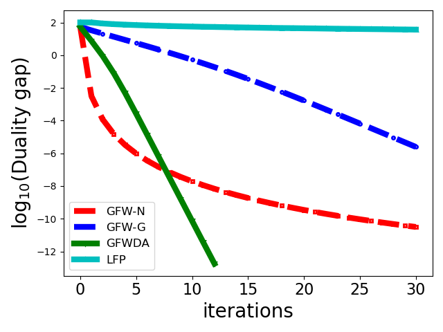
(a) Log-linear scale

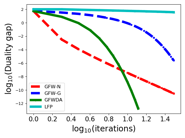
(b) Log-log scale

Figure 1: Comparison of the convergence speed of duality gaps generated by GFW-N, GFW-G, GFWDA and LFP in (a) log-linear scale and (b) log-log scale.

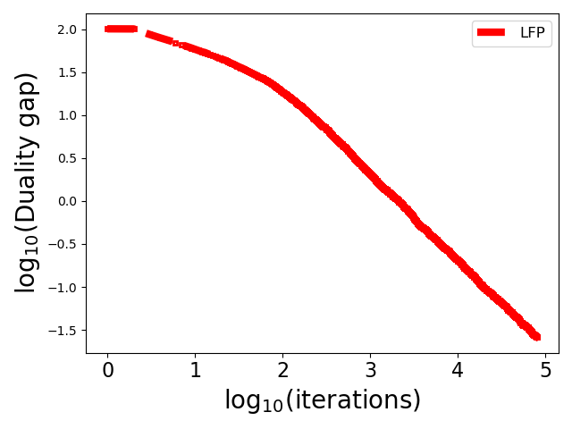
Figure 2: Log-log plot of the averaged duality-gap trajectories generated by LFP.

Iteration intervals	Slopes
$1$ to $5$	-0.229
$5$ to $5^{2}$	-0.342
$5^{2}$ to $5^{3}$	-0.590
$5^{3}$ to $5^{4}$	-0.951
$5^{4}$ to $5^{5}$	-1.030
$5^{5}$ to $5^{6}$	-0.994
$5^{6}$ to $5^{7}$	-0.991

Table 1: Slopes of the plot in Figure 2 over iteration intervals of constant lengths in log-scale.

Next, let us examine the local convergence rate of LFP. From the plot in Figure 2, we can observe an $O(1/t)$ convergence rate starting from around $100$ iterations. For better illustration, in Table 1, we compute the slopes of this plot over iteration intervals of constant lengths in log-scale. From Table 1, we can clearly see that the magnitudes of the slopes are initially very small, which correspond to the slow initial convergence of the duality gaps. However, they gradually converge to one, which correspond to the $O(1/t)$ local convergence rate as “predicted” in Theorem 4.2.

Appendix A Proof of Lemma 4.2

Let $\{\beta_{t}\}_{t\geq 0}$ be a nonnegative auxiliary sequence such that

$$\beta_{t}\geq\beta_{t+1}(1-\alpha_{t+1}),\quad\forall\,t\geq t_{0}.$$ (A.1)

As a result, we have

$$\beta_{t+1}(1-\alpha_{t+1})V_{t+1}\leq\beta_{t}(1-\alpha_{t})V_{t}+\beta_{t}\alpha_{t}^{2}C,\quad\forall\,t\geq t_{0}.$$ (A.2)

After telescoping (A.2) over $i=t_{0},\ldots,t-1$, we have

$$\beta_{t}(1-\alpha_{t})V_{t}\leq\beta_{t_{0}}(1-\alpha_{t_{0}})V_{t_{0}}+C\textstyle\sum_{i=t_{0}}^{t-1}\beta_{i}\alpha_{i}^{2},\qquad\forall\,t\geq t_{0}+1,$$

and consequently,

$$V_{t}\leq\frac{\beta_{t_{0}}(1-\alpha_{t_{0}})V_{t_{0}}}{\beta_{t}(1-\alpha_{t})}+\dfrac{C\sum_{i=t_{0}}^{t-1}\beta_{i}\alpha_{i}^{2}}{\beta_{t}(1-\alpha_{t})},\qquad\forall\,t\geq t_{0}+1,$$ (A.3)

If we choose $\alpha_{t}=2/(t+2)$ for all $t\geq 0$, to satisfy (A.1), we can then choose $\beta_{t}=(t+2)(t+1)/2$ for all $t\geq 0$. Therefore, we have

$$\beta_{t}(1-\alpha_{t})=t(t+1)/2\quad\mbox{and}\quad\textstyle\sum_{i=t_{0}}^{t-1}\beta_{i}\alpha_{i}^{2}=\sum_{i=t_{0}}^{t-1}{2(i+1)}/{(i+2)}\leq 2(t-t_{0}).$$ (A.4)

Substituting (A.4) into (A.3), we then complete the proof.

References

- [1] F. Bach, “Duality between subgradient and conditional gradient methods,” SIAM J. Optim., vol. 25, no. 1, pp. 115–129, 2015.
- [2] Y. Nesterov, “Complexity bounds for primal-dual methods minimizing the model of objective function,” Math. Program., vol. 171, pp. 311––330, 2018.
- [3] S. Ghadimi, “Conditional gradient type methods for composite nonlinear and stochastic optimization,” Math. Program., vol. 173, pp. 431––464, 2019.
- [4] J. Pena, “Affine invariant convergence rates of the conditional gradient method.” arXiv:2112.06727, 2021.
- [5] M. Frank and P. Wolfe, “An algorithm for quadratic programming,” Nav. Res. Logist. Q., vol. 3, no. 1‐2, pp. 95–110, 1956.
- [6] R. M. Freund and P. Grigas, “New analysis and results for the frank–wolfe method,” Math. Program., vol. 155, pp. 199––230, 2016.
- [7] R. Zhao and R. M. Freund, “Analysis of the frank-wolfe method for convex composite optimization involving a logarithmically-homogeneous barrier,” Math. Program., accepted, 2022.
- [8] D. Fudenberg and D. M. Kreps, “Learning mixed equilibria,” Games Econ. Behav., vol. 5, no. 3, pp. 320–367, 1993.
- [9] S. M. Kakade, S. Shalev-Shwartz, and A. Tewari, “On the duality of strong convexity and strong smoothness: Learning applications and matrix regularization,” tech. rep., TTIC, 2009. URL: https://home.ttic.edu/~shai/papers/KakadeShalevTewari09.pdf.
- [10] J. Peypouquet, Convex optimization in normed spaces : theory, methods and examples. Springer, 2015.
- [11] J. L. Ny, “On some extensions of fictitious play,” tech. rep., MIT, 2006.
- [12] J. Hofbauer and W. H. Sandholm, “On the global convergence of stochastic fictitious play,” Econometrica, vol. 70, no. 6, pp. 2265–2294, 2002.
- [13] Y. Nesterov, “Smooth minimization of non-smooth functions,” Math. Program., vol. 103, no. 1, pp. 127–152, 2005.
- [14] D. Hunter, “Lecture notes in asymptotic tools, chapter 3.” http://personal.psu.edu/drh20/asymp/fall2006/lectures/ANGELchpt03.pdf, 2006.