Quantifying quantumness of channels without entanglement

Abstract

Quantum channels breaking entanglement, incompatibility, or nonlocality are defined as such because they are not useful for entanglement-based, one-sided device-independent, or device-independent quantum information processing, respectively. Here, we show that such breaking channels are related to complementary tests of macrorealism i.e., temporal separability, channel unsteerability, temporal unsteerability, and the temporal Bell inequality. To demonstrate this we first define a steerability-breaking channel, which is conceptually similar to entanglement and nonlocality-breaking channels and prove that it is identical to an incompatibility-breaking channel. A hierarchy of quantum non-breaking channels is derived, akin to the existing hierarchy relations for temporal and spatial quantum correlations. We then introduce the concept of channels that break temporal correlations, explain how they are related to the standard breaking channels, and prove the following results: (1) A robustness-based measure for non-entanglement-breaking channels can be probed by temporal nonseparability. (2) A non-steerability-breaking channel can be quantified by channel steering. (3) Temporal steerability and non-macrorealism can be used for, respectively, distinguishing unital steerability-breaking channels and nonlocality-breaking channels for a maximally entangled state. Finally, a two-dimensional depolarizing channel is experimentally implemented as a proof-of-principle example to demonstrate the hierarchy relation of non-breaking channels using temporal quantum correlations.

I Introduction

The extension of quantum physics into the realm of information theory is important both for fundamental physics and for practical applications, such as quantum computing, quantum cryptography [1], and quantum random number generation [2, 3]. For the latter two examples, the practical implementations of entanglement based, device-independent, and one-side device-independent quantum information tasks [4, 5, 6, 7] rely on quantum resources, e.g., entangled [8, 9, 10], nonlocal [11, 12, 13, 14, 15, 16], and steerable states [17, 18, 19, 20], respectively. Extending these ideas to quantum networks [21, 22, 23, 24], one needs reliable quantum devices (e.g., quantum communication lines [25] and quantum repeaters [26, 27]) to transmit or generate quantum resources between nodes (senders and receivers) in the network.

In general, the properties of quantum networks can be characterized by the concept of quantum channels [28], which is particularly convenient for estimating the preservability of quantum resources [29]. For instance, a reliable quantum memory [30, 31] should ideally preserve the entanglement. Therefore, in channel formalism, the most useful quantum memory is the identity channel, while the threshold of a quantum memory becoming not useful is given by the entanglement-breaking (EB) channel [32, 33].

In recent years, the framework of a resource theory of quantum memories [34] has been proposed to quantify the quantumness of non-EB channels [34]. The experimental quantification [35] and practical implementation [31] of a quantum memory was demonstrated not long after [34]. These results inspired a new research paradigm around detecting a faithful quantum memory with a set of temporal quantum correlations using characterized input probing states but uncharacterized measurement apparatus [36] (see Fig. 1 for a schematic view of how to probe a non-breaking channel with temporal quantum correlations). For instance, when only the sender apparatus is trusted (such a scenario is referred to as the channel-steering scenario [37] or a semi-quantum prepare-and-measure scenario [38]), one can certify non-EB channels. More recently, sequential-measurement approaches have been proposed to detect quantum memories [39, 40] (see also the experimental realization of [41]). Another approach to witness the non-EB channel is by estimating the coherence of a state sent through the channel [42]. We emphasize that the methods introduced in these works, and in this article, are different from the typical approach, which used entanglement as a resource to detect quantumness of channels [32, 33].

Recently, nonlocality-breaking (NLB) channels [43], defined in a conceptually similar way to EB channels, were shown to be not useful for device-independent quantum information tasks. As expected from the hierarchy of correlations [44], the EB channel also breaks nonlocality, but not vice versa [43, 45]. Thus, the EB channel is a strict subset of the set of NLB channels. Although the definition of the NLB channels is rigorous, one can only assess non-NLB channels by observing a Bell inequality violation with arbitrary entangled quantum states as input.

Breaking channels	EB channel [32]	SB channel [45]	unital SB channel [45]	NLB for the MES [43]
Spatial correlations	Entanglement	Steerability	Steerability	Bell nonlocality
Temporal correlations	Temporal semi-quantum game* [34]	Channel steering* [37]	Temporal steering* [46]	Temporal Bell inequality* [47, 48]
	Temporal nonseparability* [49]	SQPM [38]
	Coherence [42]
	Sequential measurements [39, 40]

Table 1: Table showing how to probe non-breaking channels with spatial and temporal quantum correlations. Here the italics represent the results of this work and the asterisk marks the measures within the corresponding temporal scenarios satisfying the conditions for a quantum memory monotone. We note that SQPM and MES are the abbreviations of the semi-quantum prepare-and-measure scenario and the maximally entangled state, respectively.

In this work, we propose the concept of a steerability-breaking (SB) channel, which by definition is a channel that is not useful for one-sided device-independent quantum information tasks, and show that it is identical to an incompatibility-breaking channel [45]. We then introduce a measure for non-SB channels, called the robustness of the non-SB channel. This measure satisfies monotonicity in the sense that the robustness of a non-SB channel cannot increase under non-SB free operations, which map SB channels to SB channels. Similarly, we also propose a measure for non-NLB channels and demonstrate their associated monotonicity. We also complete the discussion of the relationship between SB and NLB by proving that all NLB channels must be SB channels. In addition, we show that the set of all Clauser-Horne-Shimony-Holt (CHSH) breaking channels [43, 50], which is a particular type of NLB channel, is a strict subset of all SB channels. Therefore, the hierarchy of breaking channels can be obtained.

We then focus on the quantification of breaking channels using temporal correlations without trust of the input probing states. More specifically, we connect the non-EB, non-SB, and non-NLB channels with certain temporal quantum correlations including the temporal nonseparability [49], channel steerability [37, 51], temporal steerability [46, 51], and Leggett-Garg inequalities (LGIs) [52, 53] in the form of temporal Bell inequalities [48, 47, 54, 55, 56, 57]. Then we show that: (1) temporal nonseparability can be used to measure a quantum memory [34], (2) channel steering can be used to estimate the robustness of non-SB channels, while the temporal steerability can only quantify non-SB unital channels, and (3) the robustness of non-macrorealism can bound the robustness of non-NLB channels. In the CHSH scenario, we show that all unital non-CHSH-NLB channels can be certified in the temporal domain. In Table 1, we summarize some previous observations and our new results about breaking channels and temporal quantum correlations. Finally, we experimentally demonstrate an explicit example to show not only the relationship between breaking channels and temporal quantum correlations, but also the hierarchy relationship between breaking channels.

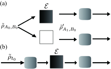
Figure 1: Schematic illustration of quantifying quantumness of channels with (a) spatial and (b) temporal quantum correlations. In (a), one relies on a bipartite quantum input $\tilde{\rho}_{A_{0},B_{0}}$ sent to an unknown channel $\mathcal{E}$ (black box). The channel can be quantified by analyzing the obtained spatial correlation of the state $\tilde{\rho}^{\prime}_{A_{1},B_{0}}$ via a quantum measurement (grey rectangle). In (b), a given property of $\mathcal{E}$ can be estimated by a temporal quantum correlation with an input $\tilde{\rho}_{t{{}_{0}}}$ which is measured before and after the channel.

II Quantum correlations and their corresponding breaking channels

In this section, we first briefly review the definitions and the properties of the EB and NLB channels. We then propose the SB channel, which is defined in conceptual analogy to the EB and NLB channels. The properties of the SB channel, including the relationship with the incompatibility-breaking channel, will also be discussed. Finally, we discuss the hierarchy relation for breaking channels.

Before showing our results, we first introduce some notations used in this work. We consider $\mathcal{L}(H_{A})$ as the set of linear operators acting on the Hilbert space $H_{A}$ with a finite dimension $d_{A}$. We denote a set of standard density operators $\mathcal{D}(H_{A})\in\mathcal{L}(H_{A})$, satisfying positive semidefiniteness and having a unit trace. A quantum channel is described by a set of completely-positive (CP) trace-preserving (TP) maps from $\mathcal{L}(H_{A})$ to $\mathcal{L}(H_{B})$ as $\mathcal{O}(H_{A},H_{B})$. Moreover, a unital map is a map that preserves the identity: $\openone\to\openone$. The set of probability distributions is denoted by $\mathcal{P(\mathcal{X})}$ with a finite index set $\mathcal{X}$. Finally, we only consider one subsystem, without loss of generality, of a bipartite quantum state $\tilde{\rho}_{A_{0},B_{0}}\in\mathcal{D}(H_{A_{0}},H_{B_{0}})$, which is sent into the quantum channel $\mathcal{E}\in\mathcal{O}(H_{A_{0}},H_{A_{1}})$, and denote the output state as $\tilde{\rho}^{\prime}_{A_{1},B_{0}}=(\mathcal{E}\otimes\openone)\tilde{\rho}_{A_{0},B_{0}}$.

II.1 Quantum memory and entanglement-breaking channel

A bipartite quantum state $\tilde{\rho}_{A_{0},B_{0}}$ shared between Alice and Bob is entangled if the corresponding density operator is not separable, namely

$$\tilde{\rho}_{A_{0},B_{0}}\neq\sum_{j}p(j)\,\tilde{\sigma}_{{A_{0}}}(j)\otimes\tilde{\eta}_{{B_{0}}}(j),$$ (1)

where $p(j)\in\mathcal{P}(\mathcal{J})$ is a probability distribution, and $\tilde{\sigma}_{{A_{0}}}(j)\in\mathcal{D}(H_{A_{0}})$ $(\tilde{\eta}_{{B_{0}}}(j)\in\mathcal{D}(H_{B_{0}}))$ is a local density operator. In general, the EB channel is defined by sending Alice’s subsystem into a quantum channel $\mathcal{E}\in O(H_{A_{0}},H_{A_{1}})$, such that the entanglement is broken for arbitrary entangled states. We can explicitly formulate the EB channel as

$$\tilde{\rho}^{\prime}_{A_{1},B_{0}}=(\mathcal{E}^{\text{EB}}\otimes\openone)(\tilde{\rho}_{A_{0},B_{0}})\in\mathcal{F}_{\text{SEP}}\leavevmode\nobreak\ \leavevmode\nobreak\ \forall\leavevmode\nobreak\ \tilde{\rho}_{{A_{0}},{B_{0}}}.$$ (2)

Here, the superscript EB is used to denote the channel $\mathcal{E}$ to be EB, and the set of separable states is denoted by $\mathcal{F}_{\text{SEP}}$.

Entanglement-breaking channels are equivalent to measure-and-prepare channels, namely

$$\mathcal{E}^{\text{EB}}(\tilde{\rho}_{{t_{0}}})=\sum_{j}\text{Tr}\left[\tilde{\rho}_{{t_{0}}}M_{j}\right]\tilde{\sigma}_{{t_{1}}}(j),$$ (3)

where $M_{j}$ is a positive-operator valued measurement (POVM) element satisfying $M_{j}>0\leavevmode\nobreak\ \forall\leavevmode\nobreak\ j$, and $\sum_{j}M_{j}=\openone$ with classical outcomes $j$. Here, with some slight abuse of notation, by $t_{0}$ ($t_{1}$) we denote a time indicating that the system is in the Hilbert space $\mathcal{H}_{t_{0}}$ ($\mathcal{H}_{t_{1}}$) before (after) the operation of the quantum channel. The physical interpretation of the EB channel can be explained as follows: one measures the original system $\tilde{\rho}_{{t_{0}}}\in\mathcal{D}(H_{t_{0}})$ at $t_{0}$, after that, based on the outcome $j$, the corresponding state $\tilde{\sigma}_{{t_{1}}}(j)\in\mathcal{D}(H_{t_{1}})$ is prepared at $t_{1}$. Obviously, when we send one of the entangled pairs into a measure-and-prepare channel, the system becomes separable since one has locally prepared another quantum state without any direct interaction with the other party.

It has been shown that a non-EB channel is a criterion for a functional quantum memory because one would like a quantum memory to, at the very least, preserve the entanglement of a state. In the framework of the resource theory of quantum memory [34, 31], one can introduce a set of quantum-memory free operations transforming any EB channel to another EB channel (see Appendix. A for more details). With these quantum-memory free operations, we can recall that the robustness of a quantum memory is the minimal noise $\alpha$ mixing with the input quantum memory, such that the whole memory is lost, namely

$$\text{R}_{\text{QM}}(\mathcal{E})=\min\left\{\alpha\;\Big{|}\frac{\mathcal{E}+\alpha\mathcal{E}^{\prime}}{1+\alpha}\in\mathcal{F}_{\text{EB}}\right\}.$$ (4)

Here, $\mathcal{E}^{\prime}$ is an arbitrary quantum channel and $\mathcal{F}_{\text{EB}}$ is the set of EB channels. It has been shown that the robustness of a quantum memory is a monotonic function after applying a quantum-memory free operation [31].

II.2 Nonlocality-breaking channel

Before introducing the notion of the NLB channel, let us briefly recall the definition of Bell nonlocality. A spatially separated state is Bell-local when local measurements with finite inputs $x\in\mathcal{X}$ ($y\in\mathcal{Y}$) and outcomes $a\in\mathcal{A}$ ($b\in\mathcal{B}$) generate a correlation $p(a,b|x,y)=\text{Tr}\left[(M_{a|x}\otimes M_{b|y})\tilde{\rho}_{A,B}\right]$ which admits a local-hidden variable (LHV) model [12, 13], namely,

$$p(a,b|x,y)=\sum_{j}p(j)p(a|x,j)p(b|y,j),$$ (5)

which the correlations are pre-determined by a hidden variable $j$. Here, we denote a set of correlations admitting a LHV model as $\mathcal{F}_{\text{LHV}}$. Since quantum correlations are a strict superset of $\mathcal{F}_{\text{LHV}}$ forming a convex set, one can distinguish the local correlation from the quantum ones by testing the famous Bell inequalities given by the parameters $\beta^{x,y}_{a,b}$ [58, 12, 13], namely

$$B\equiv\sum_{a,b,x,y}\beta^{x,y}_{a,b}\,p(a,b|x,y)\;\leq\;\delta^{\beta},$$ (6)

where $\delta^{\beta}$ is the local bound for a given Bell inequality.

Analogous to the EB channels, a NLB channel is the channel under which a correlation always satisfies a LHV model for arbitrary measurements and states, namely [43]

$$p(a,b|x,y)= \text{Tr}(M_{a|x}\otimes M_{b|y}\tilde{\rho}^{\prime}_{{A_{1}},{B_{0}}})\in\mathcal{F}_{\text{LHV}}$$ (7)

$$\forall\leavevmode\nobreak\ \{M_{a|x}\},\{M_{b|y}\},\tilde{\rho}_{{A_{0}},{B_{0}}}.$$

Similar to the definition of the robustness of a quantum memory, we now consider a noise $\alpha$ mixing with a given channel $\mathcal{E}$, namely

$$\mathcal{E}_{\alpha}=\frac{\mathcal{E}+\alpha\mathcal{E^{\prime}}}{1+\alpha}.$$ (8)

This noisy channel always generates a correlation satisfying a LHV model for arbitrary measurements and states. We denote the minimal value $\alpha$ as the robustness of the non-NLB channel $\text{R}_{\text{n-NLB}}(\mathcal{E})$. In Appendix A, we show that the robustness of a non-NLB channel is a monotonic function under a non-NLB free operation.

NLB channels have some other important known properties, which we summarize here. Unlike the situation with EB channels, the input of a maximally entangled state is not sufficient for verifying if the channel is NLB [43, 59]. In particular, because of this, we denote the case with the input being the maximally entangled state $|\Phi\rangle=\sum_{i}(1/\sqrt{d})|i\rangle\otimes|i\rangle$ as NLB channels for the maximally entangled state. In Ref. [43], the authors considered a particular NLB channel [the Clauser-Horne-Shimony-Holt (CHSH) NLB channel], i.e., channels that break CHSH-nonlocality for any state and measurements. Here, we say that a system satisfies CHSH nonlocality if it violates the CHSH inequality, namely:

$$B_{\text{CHSH}}\equiv E(x_{1},y_{1})+E(x_{2},y_{1})+E(x_{1},y_{2})-E(x_{2},y_{2})\leq 2,$$ (9)

where $2$ is the local bound for the CHSH inequality [58], $E(x_{i},y_{j})\equiv p(a=b|x_{i},y_{j})-p(a\neq b|x_{i},y_{j})$ is the expectation value of $a\cdot b$, for $a\in\mathcal{A}$, $b\in\mathcal{B}$, $x_{i}\in\mathcal{X}$, and $y_{j}\in\mathcal{Y}$, with $\mathcal{X}=\mathcal{Y}=\{1,2\}$, and $\mathcal{A}=\mathcal{B}=\{\pm 1\}$. The quantum bound of the CHSH inequality is given by $2\sqrt{2}$. We note that the CHSH-NLB channels for the maximally entangled state have the property [43]: if the channel is unital, then it is also CHSH-NLB.

II.3 Steerability-breaking channels

Now we introduce our first main result: the concept of “steerability-breaking channel” which breaks any quantum information tasks using quantum steerability as a resource. We then investigate the properties of the SB channel by showing that the channel is SB if and only if it breaks the quantum steerability of the maximally entangled state. The above property is useful not only for experimental-friendly certifications of SB, but also for the theoretical analysis of SB channels. For instance, (1) we derive that a SB channel is equivalent to the incompatible-breaking channel [45], (2) we propose the robustness as a quantification of a non-SB channel, and (3) we discuss the hierarchy relationship between breaking channels.

Quantum steering refers to the ability of remotely projecting Bob’s quantum states by Alice’s collection of measurements $\{M_{a|x}\}$ with finite inputs $x$ and outcomes $a$ [60, 18]. A set of measurements gives rise to a collection of quantum states, termed as an assemblage,

$$\rho_{B}(a|x)=\text{Tr}_{A}\left[(M_{a|x}\otimes\openone)\tilde{\rho}_{A,B}\right]$$ (10)

where $\tilde{\rho}_{A,B}$ is a bipartite state shared by Alice and Bob. We say that an assemblage is unsteerable when it admits a local-hidden-state (LHS) model, namely

$$\rho_{B}(a|x)=\sum_{j}p(j)p(a|x,j)\tilde{\rho}_{B}(j).$$ (11)

Otherwise, the assemblage is steerable. The physical interpretation of a LHS model is that an assemblage can be pre-determined by a hidden variable $j$, which simultaneously distributes over the statistics $p(a|x,j)$ and the states $\tilde{\rho}_{B}(j)\in D(H_{B})$. The set of all assemblages admitting a LHS model is denoted as $\mathcal{F}_{\text{LHS}}$. Violation of a LHS model simultaneously implies that (i) the shared state is entangled and (ii) Alice’s measurement violates incompatibility [61, 62, 63, 64]. It has been shown that quantum steering is a central resource for one-sided device-independent quantum information tasks including: metrology [65], quantum advantages on the subchannel-discrimination problems [66, 67], key distribution [7], and random number generation [68, 69, 70].

In analogy to the EB and NLB channels, we propose a SB channel as a channel which breaks the steerability for any collection of measurements $\{M_{a|x}\}$ acting on the state sent through the channel $\tilde{\rho}^{\prime}_{{A_{1}},{B_{0}}}$. More specifically, the assemblage after a SB channel can always be expressed by a LHS model, namely

$$\rho_{{B_{0}}}(a|x)=\text{Tr}_{A_{1}} \left[M_{a|x}\otimes\openone\tilde{\rho}^{\prime}_{{A_{1}},{B_{0}}}\right]\in\mathcal{F}_{\text{LHS}}\leavevmode\nobreak\$$ (12)

$$\forall\leavevmode\nobreak\ \{M_{a|x}\},\tilde{\rho}_{{A_{0}},{B_{0}}}.$$

We denote the set of all SB channels as $\mathcal{F}_{\text{SB}}$. Moreover, we define $|\mathcal{X}|$-SB channels which break the steerability with a finite input $|\mathcal{X}|$. For instance, if the finite index set is $\mathcal{X}=\{1,2,3\}$, we can define the $3$-SB channel. Here, we show that SB channels have the following properties:

Theorem 1.

A quantum channel is steerability-breaking if and only if it breaks steerability of the maximally entangled state.

Proof.—We present a proof of this theorem in Appendix B. We now use the above result to simplify the definition of the SB channel.

The definition of the SB channel is similar to that of the incompatibility-breaking channel, which maps an incompatible measurement $\{M_{a|x}\}$ to a jointly measurable one in the Heisenberg picture [45, 71]. More specifically, a set of measurements after incompatibility-breaking channel can always expressed as

$$\mathcal{E}^{\dagger}(M_{a|x})=\sum_{j}p(a|x,j)M_{j}\leavevmode\nobreak\ \leavevmode\nobreak\ \forall\leavevmode\nobreak\ \{M_{a|x}\},$$ (13)

where $\sum_{j}p(a|x,j)M_{j}$ is a joint measurable model with an intrinsic POVM $\{M_{j}\}$ and postprocessing $p(a|x,j)$. Here, $\mathcal{E}^{\dagger}$ is the dual map of the quantum channel which is CP and unital. The set of the joint measurements is denoted by $\mathcal{F}_{\text{JM}}$. Intuitively, the incompatibility-breaking channels form a proper subset of SB channels because a joint measurement cannot generate a steerable assemblage [62, 63, 64]. With Theorem 1, we provide a stronger connection between two breaking channels by the following theorem:

Theorem 2.

A quantum channel is steerability-breaking if and only if it is incompatibility-breaking.

Proof.—We present the proof in Appendix B. We recall that there is a one-to-one relation between an unsteerable assemblage and a joint measurement [64, 62, 63]. Our result provides a similar but not identical analog in terms of breaking channels. This result can be naturally extended in a quantitative manner (as shown below).

To quantify the degree of a non-SB channel, we consider, again, a noisy channel consisting of a noise $\alpha$ and the input non-SB channel $\mathcal{E}$ [cf. Eq. (8)]. The standard robustness of the non-SB channel is defined as the minimal value of the noise $\alpha$, such that the whole channel is SB for any measurement set $\{M_{a|x}^{\text{T}}\}$ and any entangled state, namely

$$\text{R}_{\text{n-SB}}(\mathcal{E})=\min\{\alpha\big{|}\text{Tr}_{A_{1}}[M^{\text{T}}_{a|x}\otimes\openone\mathcal{E}_{\alpha}(\tilde{\rho}_{{}_{{A_{0}},{B_{0}}}})]\in\mathcal{F}_{\text{LHS}}$$ (14)

$$\leavevmode\nobreak\ \forall\tilde{\rho}_{{}_{{A_{0}},{B_{0}}}},M^{\text{T}}_{a|x}\leavevmode\nobreak\ \},$$

where T denotes the transposition. Inserting the maximally entangled state $|\Phi\rangle=\sum_{i}(1/\sqrt{d})|i\rangle\otimes|i\rangle$ (Theorem 1) into Eq. (14) , we can simplify the standard robustness of the non-SB channel in the Heisenberg picture to arrive at

$$\text{R}_{\text{n-IB}}(\mathcal{E})=\min\left\{\alpha\Big{|}\frac{\left[\mathcal{E}^{\dagger}+\alpha\mathcal{E^{\prime}}^{\dagger}\right]}{1+\alpha}(M_{a|x})\in\mathcal{F}_{\text{JM}}\leavevmode\nobreak\ \forall\leavevmode\nobreak\ \{M_{a|x}\}\right\}.$$ (15)

Here, we use the fact that $(\mathbf{X}\otimes\mathbf{Y})|\Phi\rangle\langle\Phi|=\mathbf{X}\mathbf{Y}^{\text{T}}\otimes\openone|\Phi\rangle\langle\Phi|$, where $\mathbf{X}(\mathbf{Y})$ is any operator, and the subscript in $\text{R}_{\text{n-IB}}$ is used to denote the non-incompatibility-breaking channels. One can see that Eq. (15) is the same as the robustness of the non-incompatiability-breaking channel proposed in Ref. [38]. In Appendix A, we further show that the robustness of a non-SB channel is a monotonic function under the most general non-SB free operation.

It has been shown that the sets of all incompatibility-breaking channels (also SB channels) and NLB channels are both supersets of the set of all EB channels [43, 45]. To complete this hierarchy relationship between breaking channels, we show the following:

Theorem 3.

The set of all non-EB, non-SB, non-NLB, and non-CHSH-NLB channels form a strict hierarchy. More specifically, we have the strict inclusions

$$\mathcal{F}_{\text{EB}}\subset\mathcal{F}_{\text{SB}}\subset\mathcal{F}_{\text{NLB}}\subset\mathcal{F}_{\text{NLB}_{\text{CHSH}}}.$$ (16)

Proof.—We present the proof of Theorem 3 in Appendix D, and we illustrate this theorem for the qubit depolarizing channel

$$\mathcal{E}_{\text{D}}(v,\tilde{\rho})=v\tilde{\rho}+(1-v)\frac{\openone}{2}$$ (17)

in Fig. 2. The experimental demonstration of this theorem is also presented in Sec. IV. We note that $\mathcal{F}_{\text{NLB}_{\text{CHSH}}}$ denotes the set of CHSH-NLB channels.

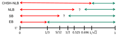
Figure 2: Visibility parameter $v$ for which the qubit depolarizing channel is CHSH-nonlocality breaking, nonlocality-breaking (NLB), steerability-breaking (SB), and entanglement-breaking (EB). The first bar in red represents the range, where the channel is proven to break the property, and the second bar in green shows the range, where the channel is proven not to break the property. The white areas with a question mark represent the ranges where the property is not known to be broken.

III Quantifying quantum non-breaking channels with temporal quantum correlations

In this section, we present our second main result regarding probing the robustness of non-breaking channels with temporal quantum correlations. In section III.1, we show that all EB channels are temporally separable and one can probe $\text{R}_{\text{QM}}$ with temporal nonseparability. In section III.2, we show that all the non-SB channels can be quantified by testing channel steerability. In section III.3, temporal steering and the Leggett-Garg inequality are used to test whether a channel is non-SB and non-NLB, respectively.

Before presenting our results, it is useful to recall the Choi-Jamiołkowski (CJ) isomorphism [72, 73], which is a one-to-one mapping between a quantum channel and a positive semidefinite operator. A CJ state $\tilde{\rho}^{\text{CJ}}_{\mathcal{E}}\in D(H_{t_{0}}\otimes H_{t_{1}})$ of a quantum channel $\mathcal{E}\in O(H_{t_{0}},H_{t_{1}})$ is defined as

$$\tilde{\rho}^{\text{CJ}}_{\mathcal{E}}=(\openone\otimes\mathcal{E})|\Phi\rangle\langle\Phi|,$$ (18)

where $|\Phi\rangle$ is the maximally entangled state. The output state under the Choi representation is formulated as $\mathcal{E}(\mathbf{X})=\text{Tr}_{t_{0}}\left[(\openone\otimes\mathbf{X}^{\text{T}})\tilde{\rho}^{\text{CJ}}_{\mathcal{E}}\right]$, with $\mathbf{X}$ being any operator. Note that the quantum state and the quantum channel can be converted with each other with the Choi representation [72, 73]. Finally, it has been shown that a CJ state is separable if and only if the corresponding channel is EB [32, 74].

III.1 Quantifying a non-EB channel with temporal quantum correlations

We first briefly recall the definition of a pseudo-density operator (PDO), which has primarily been used in the study of the causality of quantum theory [49]. We then show that the temporal nonseparability extracted from a PDO can be used to measure the quality of a quantum memory. Afterwards, we show that the PDO formalism is operationally equivalent to the formalism of temporal semi-quantum games in the task of verifying non-EB channels [34].

To reconstruct the state of a quantum system from trusted measurements performed at different times, one can generalize the concept of a standard density operator in the time domain [49] (see also Fig. 3). Without loss of generality, the events, or observations, collated at different times can be connected by quantum channels to an input state. In what follows, we only consider a two-event PDO with a maximally mixed input. The information of a channel is contained in the PDO, namely [75]

$$P_{\mathcal{E}}=(\openone\otimes\mathcal{E})P_{\mathcal{\openone}},$$ (19)

where $P_{\mathcal{\openone}}=\text{SWAP}/d$ is the PDO of the identity channel with the swap operator defined by $\text{SWAP}|ij\rangle=|ji\rangle$. For the qubit case, we have $\text{SWAP}=1/2\sum_{i=0}^{3}\sigma_{i}\otimes\sigma_{i}$. Here, $\{\sigma_{i}\}_{i=0,1,2,3}=\{\openone,\hat{X},\hat{Y},\hat{Z}\}$ is a set containing the identity and Pauli operators. A PDO is: (1) Hermitian and (2) unit trace but not necessarily positive semidefinite (the latter is a necessary condition for a standard density operator). Similar to the standard density operator, a PDO is called temporally separable when it admits

$$P_{\mathcal{E}}=\sum_{j}p(j)\,\tilde{\omega}_{{t_{0}}}(j)\otimes\tilde{\theta}_{{t_{1}}}(j),$$ (20)

where $p(j)\in\mathcal{P}(\mathcal{J})$, $\tilde{\omega}_{{t_{0}}}(j)\in D(H_{t_{0}})$, and $\tilde{\theta}_{{t_{1}}}(j)\in D(H_{t_{1}})$. In Eq. (20), there exist definite states described by $\tilde{\omega}_{{t_{0}}}(j)$ and $\tilde{\theta}_{{t_{1}}}(j)$ at each moment of time, $t_{0}$ and $t_{1}$.

It has been shown that the PDO is identical to the partial transpose of the CJ state of the channel $\mathcal{E}$ [76, 77],

$$P_{\mathcal{E}}^{\text{PT}}=\tilde{\rho}^{\text{CJ}}_{\mathcal{E}},$$ (21)

where PT is the partial transposition with respect to the first subsystem. Therefore, a separable PDO implies that the CJ state is also separable and, thus, the corresponding channel must be EB [32, 74]. With the above properties, we have the following:

Lemma 1.

The partial transposition of the PDO is separable if and only if the corresponding channel is EB.

Recall that one can still use the PDO to distinguish the temporal and spatial correlations, while the partial transposition of the PDO cannot [49]. To quantify the degree of a quantum memory with a PDO, we can use again the idea of robustness-based measure. Namely, the robustness of a quantum memory is equal to the minimum ratio of a noisy operator one has to mix with the partial transpose of the PDO before the mixture becomes separable. In fact, it can be easily shown that such a measure is the same as the measure derived from the channel formalism in Eq. (4) [31].

Finally, it is useful to compare the PDO and the temporal semi-quantum scenario, which certifies all non-EB channels with minimal assumptions in the sense that only state preparation devices are trusted [34]. In detail, the temporal semi-quantum scenario is constructed by an unknown joint measurement, a given quantum channel $\mathcal{E}$, and a set of trusted states. In the beginning, one chooses a quantum state from the set as an input to the quantum channel. A joint measurement is performed on the output state and a state chosen from the same set. One can certify an arbitrary non-EB channel if the set is tomographically complete. From the PDO perspective, we now consider a set of trusted measurements $\{M_{a|x}\}$ at $t_{0}$ acting on the PDO, which is used for generating a set of states $\tilde{\rho}_{\mathcal{E}}(a|x)\in\mathcal{D}(H_{t_{1}})=\text{Tr}_{t_{0}}\left[M_{a|x}\otimes\openone P_{\mathcal{E}}\right]$, up to renormalization, at $t_{1}$ [78]. This is the so-called “normalized” temporal assemblage, and we will formally introduce it later. The joint measurement is then performed on a characterized quantum input $\{\tilde{\tau}_{y}\}\in\mathcal{D}(H_{t^{\prime}_{1}})$ and the normalized temporal assemblage. The above steps are exactly the same as the procedure used in temporal semi-quantum games, and we have

Lemma 2.

The PDO formalism is operationally equivalent to the temporal semi-quantum scenario.

Proof.—We present a detailed comparison in Appendix C. We note that, although in Ref. [50] the authors have already shown the relationship between the PDO formalism and the temporal semi-quantum scenario, we provide a clearer physical interpretation in the proof by using the property found in Ref. [78].

III.2 Certifying non-SB channels with channel steering

Here, we first recall the concept of channel steering from a PDO perspective. In this way, we can show the relationship between channel steering and non-SB channels in a quantitative manner. This will allow us to measure all non-SB channels in the temporal domain. We do not consider the more general case of channel steering used in Ref. [37] because there it is employed to discuss the coherent properties of an extended channel, which is beyond the scope of this work.

In the PDO formalism, the measurements performed at two moments of time are assumed to be characterized. Now, we replace the characterized measurement at time $t_{1}$ with an uncharacterized one with finite inputs $y\in\mathcal{Y}$ and outcomes $b\in\mathcal{B}$ (see also Fig. 3). In short, the measurements at times $t_{0}$ and $t_{1}$ are trusted and untrusted, respectively. We note that the above scenario is channel steering [37] with only classical outputs (measurement results) at time $t_{1}$. To put it another way, the measurements at $t_{1}$ on the PDO generate a set of evolved states by

$$\text{Tr}_{{t_{0}}}\left[\openone\otimes M_{b|y}P_{\mathcal{E}}\right]=\mathcal{E}^{\dagger}(M_{b|y})/d,$$ (22)

where $d$ is the dimension of the PDO. Note that the resulting state can be seen as the evolution of the measurement in the Heisenbeg picture. Since Eq. (22) is a valid assemblage, one can test whether Eq. (22) admits a hidden-state (HS) model, i.e.,

$$\mathcal{E}^{\dagger}(M_{b|y})/d=\sum_{j}p(j)p(a|x,j)\tilde{\rho}_{B}(j).$$ (23)

The above formula suggests that once the HS model is satisfied, the corresponding measurement set $\{\mathcal{E}^{\dagger}(M_{b|y})\}$ is jointly measurable (see also Appendix B). By Theorem 2, if the dual channel breaks the incompatibility of an arbitrary measurement set $\{M_{b|y}\}$, the channel is SB. Therefore, one can use channel steering to certify all SB channels. We also note that if one inserts an EB channel into Eq. (22), the assemblage also satisfies the HS model. However, due to Theorem 3, not all EB channels can be witnessed with channel steering [36].

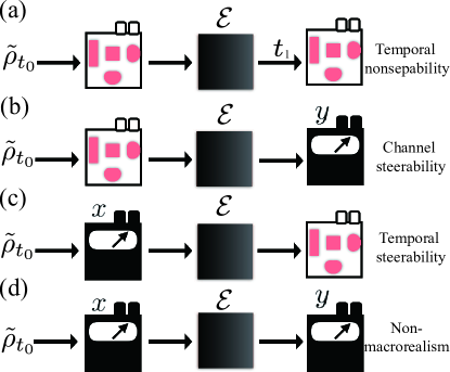
Figure 3: Schematic illustration of (a) temporal nonseparability, (b) channel steerability, (c) temporal steerability, and (d) temporal Bell inequality. Here, characterized (uncharacterized) measurements are represented by transparent (black) box. The indices $x\in\mathcal{X}$ ($y\in\mathcal{Y}$) and $a\in\mathcal{A}$ ($b\in\mathcal{B}$) denote the inputs and outcomes of the black box.

We now define the robustness of channel steering, $\text{R}_{\text{CS}}$, as the minimal ratio $\alpha$ of noise mixed with the dual map of the underlying channel such that the evolved assemblage admits a HS model, or, equivalently, the evolved measurement assemblage admits a jointly measurable model, i.e.,

$$\text{R}_{\text{CS}}(\mathcal{E},\{M_{b|y}\})=\min\left\{\alpha\Big{|}\frac{\left[\mathcal{E}^{\dagger}+\alpha\mathcal{E^{\prime}}^{\dagger}\right](M_{b|y})}{1+\alpha}\in\mathcal{F}_{\text{JM}}\right\}.$$ (24)

If we now test all incompatible measurements $\{M_{b|y}\}$ in the robustness of channel steering, the minimal one corresponds to the robustness of the non-SB channel in Eq. (15) and we arrive at:

Theorem 4.

The robustness of the non-steerability-breaking channel or, equivalently, non-incompatible-breaking channels can be quantified by the robustness of channel steering.

III.3 Certifying non-SB and non-NLB channels for maximally entangled states with temporal correlations

Here, we introduce the last two temporal scenarios: (1) the temporal analogy of quantum steering (temporal steering) and (2) non-macrorealism in the form of the temporal Bell inequality. Both scenarios can be derived from the assumptions of macrorealism (in the sense that the system is assumed to have well defined pre-existing properties (realism) and can be measured without disturbance (non-invasiveness) [53]). Beyond quantifying non-Markovianity [79, 80, 81] and connections to the security of quantum key distribution [82] , we show that temporal steerability can be used to quantify the unital non-SB channels. We also establish for the first time a link between two previously close but not directly related concepts: Bell nonlocality and non-macrorealism. In particular, we show that the value of non-macrorealism provides a lower bound on the magnitude of the non-NLB channel. In other words, if the Leggett-Garg inequality (LGI) can be violated, there exists a corresponding violation of the Bell scenario with the same measurement sets and channel.

In the temporal steering scenario, we consider a set of uncharacterized measurements with finite inputs $x\in\mathcal{X}$ and outcomes $a\in\mathcal{A}$ at $t_{0}$, while measurements at $t_{1}$ are assumed to be fully characterized (see Fig. 3). With the above setting, one can obtain a set of subnormalized quantum states, termed a temporal assemblage [46], namely

$$\rho_{\mathcal{E}}(a|x)=\text{Tr}_{t_{0}}\left[M_{a|x}\otimes\openone P_{\mathcal{E}}\right].$$ (25)

We say that a temporal assemblage is temporally unsteerable when it admits an HS model:

$$\rho_{\mathcal{E}}(a|x)=\sum_{j}p(j)p(a|x,j)\tilde{\rho}_{B}(j)$$ (26)

[c.f. Eq. (11)]. In general, an HS model in the temporal domain pre-assigns ontic probability and states in an asymmetric way, such that the system is well defined. For brevity, whenever there is no ambiguity we denote the assemblage $\{\rho_{\mathcal{E}}(a|x)\}$ as $\vec{\rho}_{\mathcal{E}}$. It is convenient to quantify the degree of temporal steerability by the robustness of temporal steerability [83, 84], which again refers to the minimum noise $\alpha$ mixed with a given assemblage before the mixture admits an HS model:

$$\text{R}_{\text{TS}}(\vec{\rho}_{\mathcal{E}})=\min\left\{\alpha\Big{|}\frac{\rho_{\mathcal{E}}(a|x)+\alpha\sigma(a|x)}{1+\alpha}\in\mathcal{F}_{\text{HS}}\right\},$$ (27)

where $\vec{\sigma}$ is an arbitrary assemblage.

From Eq. (25) and the definition of the PDO, one immediately sees that the temporal assemblage $\vec{\rho}_{\mathcal{E}}$ can be formulated as

$$\rho_{\mathcal{E}}(a|x)=\mathcal{E}(M_{a|x})/d.$$ (28)

Because now the quantum channel is acting on the measurement, in what follows we only consider the unital quantum channel denoted as $\mathcal{E}_{\text{unital}}$. It is easy to see that the set of quantum channels is a superset of the unital quantum channels. Obviously, if $\text{R}_{\text{TS}}(\vec{\rho}_{\mathcal{E_{\text{unital}}}})=0$ when considering an arbitrary measurement set $\{M_{a|x}\}$, then the channel $\mathcal{E}_{\text{unital}}$ is a unital SB channel. With Theorem 1, we can certify all unital SB channels with temporal steering. Furthermore, $\text{R}_{\text{TS}}(\vec{\rho}_{\mathcal{E}_{\text{unital}}})$ provides a lower bound on the $\text{R}_{\text{n-SB}}(\mathcal{E}_{\text{unital}})$ in Eq. (15). If the entire measurement set $\{M_{a|x}\}$ is considered, we have $\text{R}_{\text{TS}}(\vec{\rho}_{\mathcal{E}_{\text{unital}}})=\text{R}_{\text{n-SB}}(\mathcal{E}_{\text{unital}})$. We arrive at:

Theorem 5.

The robustness of temporal steerability can be used to quantify unital non-SB channels.

Let us now turn our attention to the temporal Bell scenario (see Fig. 3), which is equivalent to the LGI scenario. The measurements at both times $t_{0}$ and $t_{1}$ are viewed as black boxes with finite inputs $x\in\mathcal{X}$ and $y\in\mathcal{Y}$, respectively. The index $a\in\mathcal{A}$ ($b\in\mathcal{B}$) is used to denote the measurement outcome at $t_{0}$ ($t_{1}$) [48, 47, 53]. The system is assumed to obey the aforementioned macrorealism, which implies that a temporal correlation can be described by a hidden-variable (HV) model, namely

$$p(a,b|x,y)\stackrel{{\scriptstyle\text{MS}}}{{=}}\sum_{j}p(j)p(a|x,j)p(b|y,j).$$ (29)

One can see that the hidden parameter $j$ causally determines the well-defined probability distributions $p(a|x,j)$ and $p(b|y,j)$ at times $t_{0}$ and $t_{1}$, respectively. The violation of the temporal Bell inequality, which has the same form of Eq. (6) but with the correlation obtained from temporally separated measurements, reveals a quantum correlation effect. This quantum correlation is interpreted as non-macrorealism. This is because the temporal Bell inequality is a special kind of LGI, which is compatible with all macrorealistic physical theories.

In quantum theory, the observed correlation can be described by

$$p(a,b|x,y) =\text{Tr}\left[(M_{a|x}\otimes M_{b|y})P_{\mathcal{E}}\right]$$ (30)

$$=\text{Tr}\left[M_{b|y}\rho_{\mathcal{E}}(a|x)\right].$$

One can note that certifying the non-macrorealistic probability distribution is mathematically identical to witnessing the locality of the CJ state in Eq. (30). If the observed correlation admits an HV model, the channel breaks nonlocality for the maximally entangled states by definition. Now, we define the robustness of non-macrorealism as

$$\text{R}_{\text{n-MR}}(p(a,b|x,y))=\$$ (31)

$$\min\left\{\alpha\Big{|}\frac{p(a,b|x,y)+\alpha p^{\prime}(a,b|x,y)}{1+\alpha}\in\mathcal{F}_{\text{HV}}\right\},$$

where $\mathcal{F}_{\text{HV}}$ denotes the set of temporal correlations admitting an HV model. We can see that $\text{R}_{\text{n-MR}}$ provides a lower bound for $\text{R}_{\text{n-NLB}}$. Therefore, we have:

Theorem 6.

The robustness of non-macrorealism can be used to quantify non-NLB channels for the maximally entangled state.

Since other works [43, 59] focused on CHSH-NLB channels, we briefly discuss the particular case of the temporal CHSH inequality. Since the unital channel is CHSH-NLB, when the channel breaks the CHSH nonlocality for the maximally entangled states, the temporal CHSH inequality can be used to certify all unital CHSH-NLB channels. Finally, we emphasize that due to the hierarchy relation of temporal quantum correlations [78, 51], temporal separability implies macrorealism, but not vice versa. Thus, the concept of non-macrorealism can be used to witness non-EB channels. A similar argument for certifying non-SB channels can also be applied for testing non-macrorealism.

IV Experimental setup and results

In this section, we present a proof-of-principle experiment demonstrating (i) the hierarchy of breaking channels and (ii) how temporal quantum correlations can be used to quantify the quantumness of channels. In detail, we consider the 2-dimensional depolarizing channel, which is a convex combination of white noise with the input state, namely,

$$\mathcal{E}_{\text{D}}(v,\tilde{\rho})=v\tilde{\rho}+(1-v)\frac{\openone}{2},$$ (32)

where $v$ is the mixing parameter. The corresponding PDO can be expressed as

$$P_{\mathcal{E}_{\text{D}}}=\frac{v}{2}\text{SWAP}+\frac{1-v}{4}\openone,$$ (33)

In the temporal steering scenario, we consider the three dichotomic measurements ($\{\hat{X},\hat{Y},\hat{Z}\}$) applied on the PDO at $t_{0}$ in order to obtain the maximal temporal steerability [85, 86]. To obtain the robustness of non-macrorealism for the 2-dimensional depolarizing channel, we consider the two sets of anti-commuting operators: $\{\hat{X},\hat{Z}\}$ and $\{(\hat{X}+\hat{Z})/2,(\hat{X}-\hat{Z})/2\}$, which maximizes violation of the temporal CHSH inequality.

We have demonstrated all of these temporal scenarios in a photonic experiment. The experimental setup is schematically shown in Fig. 4. In this experiment, qubits are encoded into the polarization state of individual photons and manipulated using linear optics. More details on the experimental implementation are provided in Appendix E.

A quarter and half-wave plates are used to prepare single photons in the desired polarization state. In our experiment, we prepared six different initial states which are the eigenstates of operators $\{\hat{X},\hat{Y},\hat{Z}\}$. This preparation is operationally equivalent to the nondestructive projective measurement at $t_{0}$. The photons then enter the depolarizing channel consisting of two beam displacer assemblies (BDA), one of which is enveloped by Hadamard gates ($\hat{H}$). These two BDAs together can perform one of following operations: $\{\openone,\hat{X},\hat{Y},\hat{Z}\}$. We assign each operation a probability depending on the parameter $v$. To implement the depolarizing channel, we randomly (with assigned probabilities) with frequency 10 Hz change the operation and accumulate signal for sufficiently long times (100s) (see further details in Appendix E). To analyze the output state, we implement polarization projection and subsequent detection using a half and quarter-wave plate, a polarizer and a single photon detector. Note that the aforementioned half-wave plate is used to implement both the second Hadamard gate and the analysis. All combinations of input states together with projections onto the eigenstates of the $\{\hat{X},\hat{Y},\hat{Z}\}$ operators allows to perform a full process tomography which characterizes the entire channel in terms of the PDO.

Our experimental results are plotted in Fig. 5. As can be seen, the PDO can be used to measure quantum memory in the form of the robustness-based measure. Moreover, the PDO is separable when $v\leq 1/3$, which saturates the bound of the EB channel in the quantum domain [34]. For the temporal steering and temporal Bell scenarios, each value in Fig. 5 provides a lower bound on the robustness of the non-SB and the non-NLB channels. One can see that for the depolarizing channel, the vanishing parameter $v$ of the SB channel in the quantum domain is $v=1/\sqrt{3}$. This vanishing parameter under the three measurements setting scenario is identical to that in the $3$-incompatibility-breaking channel, which breaks the incompatibility of every collection of three measurements [45]. In other words, we can also say that it is the $3$-SB channel which breaks the spatial steerability under all of the three measurement settings. Finally, the robustness of the non-NLB channel suggests that under the two binary inputs scenario, the vanishing parameter is $v=1/\sqrt{2}$, which is identical to the boundary of the CHSH-NLB channel under the 2-dimensional depolarizing channel [43, 59]. Our experimental results also show the hierarchy between breaking channels (see also Fig. 2). The error of all experimentally obtained quantities is estimated by assuming the Poisson distribution of the photon counts. Errors of quantities obtained from the density matrices is determined by a Monte-Carlo method. Further details are given in Appendix E.

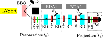
Figure 4: Scheme for our experimental implementation of the depolarizing channel. The $\beta$-Ba(BO₂)₂ is a nonlinear crystal for spontaneous parametric down-conversion; $\lambda/2$ and $\lambda/4$ are half- and quarter-wave plates, respectively; BDs are beam displacers; BDAs are beam-displacer assemblies; Pol is a polarizer; and Det are single-photon detectors.

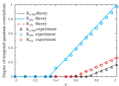
Figure 5: Effects of the 2-dimensional depolarizing channel, characterized by the mixing parameter $v$ in Eq. (32), on the robustness-based measures including: quantum memory (blue squares and solid line), temporal steerability (red circles and dashed line) and non-macrorealism (black triangles and dotted line). The experimental results are marked by symbols. The vanishing parameter of the robustness of quantum memory is $1/3$, which distinguishes the EB channel in the quantum domain. Moreover, for the temporal steering and CHSH scenarios, the vanishing parameters are respectively $1/\sqrt{3}$ and $1/\sqrt{2}$, which are the same as the boundaries of the 2-dimensional depolarizing channels for the SB and CHSH-NLB channels under the three and two dichotomic measurement settings.

V Discussion and conclusions

In this work, we have proposed the steerability-breaking (SB) channel, which is defined in an analogous way to the entanglement-breaking (EB) and nonlocality-breaking (NLB) channels. We have then proven a strict hierarchy between these concepts and experimentally illustrated it with the qubit depolarizing channel in a photonics system. We then proposed the robustness-based measures to quantify the degree of different types of non-breaking channels. In the Heisenberg picture, we can formally show that many well-known aspects concerning the incompatibility-breaking channels are equivalent with the corresponding ideas in the SB channel, including the mathematical description and robustness-based measures.

We have also connected the non-breaking channels with non-macrorealism, which is the basis of the Leggett-Garg inequality, normally used to check for quantum effects in macroscopic systems. More specifically, we have shown that the robustness-based measures of the non-EB and non-SB channels can be accessed by temporal nonseparability and channel steerability, respectively. The temporal steerability and non-macrorealism can be applied to quantify the unital non-SB channel and the non-NLB channel for the maximally entangled state. We also showed that all unital non-CHSH-NLB channels which only break the CHSH nonlocality instead of the general nonlocality can be certified by the temporal CHSH inequality. Therefore, the above breaking channels can be quantified in the temporal domain without an entangled source. We have also demonstrated the photonics experiment to explicitly show how temporal quantum correlations can be used to quantify the non-breaking channels.

Several natural questions can be discussed: Can all non-NLB channels be certified in the temporal scenario? Similar to the temporal semi-quantum game, which certifies all non-EB channels in the measurement-device-independent scenario, the measurement-device-independent channel steering has been proposed [87], but without considering the relationship with SB channels. Can measurement-device-independent channel steering certify all non-SB channels? A recently proposed loophole-free test of macrorealism [88] motivates us to ask whether we can generalize their setup and extend to a loophole-test of non-breaking channels with temporal quantum correlations? Is the negativity-like measure using the temporal nonseparability a useful quantum-memory monotone? It has been shown that the negativity-like measure of the temporal nonseparability can be used to quantify quantum causality [49] and to estimate channel capacity [75]. We have partially addressed this question by showing that the negativity-like measure of the temporal nonseparability is a lower bound of the negativity of a quantum channel [75], for which we prove that it satisfies the conditions of a quantum memory monotone under the assumption in Appendix F. In other words, the negativity-like measure of the temporal nonseparability can be used to quantify quantum memory.

Appendix A Robustness-based measures of breaking channels

We first briefly introduce the concept of a resource theory. In general, a resource theory is consisted of three components: (i) a set of free states $\mathcal{F}$, (ii) a set of free operations $\mathcal{O}$, and (iii) resource measures $Q$. Here, we only consider the most general free operations (resource-non-generating maps) and denote them as the resource-free operations for convenience. They map free states to free states. Once the free states and operations are established, we can define a resource measure (or a resource monotone) $Q$ , which obeys:

• It vanishes for any free state:

  $$Q(\mathcal{E})=0\quad\text{if}\quad\mathcal{E}\in\mathcal{F}.$$ (34)

• It is non-increasing under free operations, i.e.,

  $$Q\left(\Lambda(\mathcal{E})\right)\leq Q(\mathcal{E}),$$ (35)

  where $\Lambda$ is a free operation.

• Given a distribution $p(i)$ and resources $\mathcal{E}_{i}$, we say that $Q$ is a convex monotone if it satisfies the inequality

  $$Q\left(\sum_{i}p(i)\mathcal{E}_{i}\right)\leq\sum_{i}p(i)Q(\mathcal{E}_{i}).$$ (36)

In a resource theory, the robustness-based measure is often used because the quantity itself also directly tells us the degree of advantages that the underlying quantum object provides (see how it can be applied to general resource theories [89, 90, 91] and some explicit applications to quantum theories  [92, 93, 94, 95]). By definition, a robustness-based measure denotes how much noise can be added to the input resource before the output resource becomes free. In Table. 2, we summarize the notations of the robustness-based measure, that we considered . In what follows, we apply the above concepts to entanglement-breaking (EB), nonlocality-breaking (NLB), and steerability-breaking (SB) channels.

Table 2: Table of symbols of different robustness-based measures. The first column represents different quantum objects/phenomena discussed in our work. The second column describes the symbols used for representing the associated robustness-based measures. The third column indicates the equations where the measures appear.

quantum objects	symbols of measures	appearance
quantum memory	$\text{R}_{\text{ QM}}$	Eq. (4)
non-nonlocality breaking channel	$\text{R}_{\text{n-NLB}}$	Eq. (8)
non-steerability breaking channel	$\text{R}_{\text{n-SB}}$	Eq. (14)
channel steering	$\text{R}_{\text{CS}}$	Eq. (24)
temporal steering	$\text{R}_{\text{TS}}$	Eq. (27)
non-macrorealism	$\text{R}_{\text{n-MR}}$	Eq. (31)

A.1 Quantum memory

As mentioned in the main text, the free states of a resource theory of quantum memory is the set of EB channels [34, 31]. In Ref. [31], it has been shown that the robustness of the quantum memory $\text{R}_{\text{QM}}$ defined in Eq. (4) satisfies the quantum memory monotone, in the sense that it is a non-increasing function under quantum-memory free operations. Readers can find a more detailed discussion in Ref. [31]. Instead of the most general free operations, we discuss a particular choice of free operations proposed in Appendix F.

A.2 Nonlocality-breaking channel

Here, we first define the most general free operations within the resource theory of non-NLB-breaking channels, as the non-NLB free operations $\Lambda_{\text{NLB}}$. It is the physical transformation of quantum channels (quantum supermap) that maps NLB channels into (same or other) NLB channels only,

$$\mathcal{O}_{\text{NLB}}=\{\Lambda_{\text{NLB}}:\Lambda_{\text{NLB}}(\mathcal{E})\in\mathcal{F}_{\text{NLB}},\forall\mathcal{E}\in\mathcal{F}_{\text{NLB}}\}.$$ (37)

By defining a noisy channel, $E_{\alpha}=\frac{\mathcal{E}+\alpha\mathcal{E^{\prime}}}{1+\alpha}$, with $\mathcal{E}^{\prime}$ being any channel, we can recall that the robustness of a non-NLB channel is defined as

$$\text{R}_{\text{n-NLB}}(\mathcal{E})=\min\{\alpha\geq 0\Big{|}$$ (38)

$$\text{Tr}\left[(M_{a|x}\otimes M_{b|y})(E_{\alpha}\otimes\openone)\tilde{\rho}_{\text{A,B}}\right]\in\mathcal{F}_{\text{LHV}}\leavevmode\nobreak\ \forall M_{a|x},M_{b|y},\tilde{\rho}_{\text{A,B}}\}.$$

Here, $\mathcal{F}_{\text{LHV}}$ is a set of local correlations admitting the HV model defined in (5). By definition, one can see that the optimal channel $\mathcal{E}_{\alpha^{*}}$ is a NLB-breaking channel. In what follows, we show that the robustness of a non-NLB channel, defined in (8), is a non-NLB monotone.

Lemma 3.

The value of the robustness of a non-NLB channel is zero when the channel is NLB.

Proof.— This follows directly from the definition in Eq. (38). $\square$

Lemma 4.

The robustness of a non-NLB channel is decreasing under the non-NLB free operations.

Proof.— We first denote the optimal solution in (38) with an asterisk. Since the non-NLB free operation is linear, after applying it to $\mathcal{E}^{*}_{\alpha}$, we have

$$\Lambda\left(\frac{\mathcal{E}+\alpha^{*}\mathcal{E^{\prime}}}{1+\alpha^{*}}\right)=\frac{\Lambda(\mathcal{E})}{1+\alpha^{*}}+\frac{\alpha^{*}\Lambda(\mathcal{E^{\prime}})}{1+\alpha^{*}}=\Lambda(\mathcal{E}_{\alpha^{*}})\in\mathcal{F}_{\text{NLB}}.$$ (39)

Here, we use the property of the non-NLB operation in (37). Because $\Lambda(\mathcal{E}_{\alpha^{*}})$ is still an NLB channel, the constraints in (38) are always satisfied. However, $\alpha^{*}$ is not necessarily the minimum of $\text{R}_{\text{n-NLB}}(\Lambda(\mathcal{E}))$. Therefore, we conclude that $\text{R}_{\text{n-NLB}}(\Lambda(\mathcal{E}))\leq\text{R}_{\text{n-NLB}}(\mathcal{E})$. $\square$

Lemma 5.

The robustness of the non-NLB channel satisfies convexity, namely

$$\text{R}_{\text{n-NLB}}\left(\sum_{i}p(i)\mathcal{E}_{i}\right)\leq\sum_{i}p(i)\text{R}_{\text{n-NLB}}(\mathcal{E}_{i}).$$ (40)

Proof.— For each $i$, the solution in (38) is denoted by $\alpha_{i}^{*}$ and the channel is denoted as $\mathcal{E}^{\prime}_{i}$. According to the definition in Eq. (38), we have

$$\frac{\mathcal{E}_{i}}{1+\alpha_{i}^{*}}+\frac{\alpha_{i}^{*}\mathcal{E}^{\prime}_{i}}{1+\alpha_{i}^{*}}=\mathcal{E}_{\alpha_{i}^{*}}\in\mathcal{F}_{\text{NLB}}.$$ (41)

We now define the coefficients $\alpha=\sum_{i}p(i)\alpha_{i}^{*}$, $\mathcal{E}=\sum_{i}p(i)\mathcal{E}_{i}$, and $\mathcal{E}^{\prime}=1/\alpha\sum_{i}p(i)\alpha_{i}^{*}\mathcal{E}^{\prime}_{i}\in\mathcal{F}_{\text{NLB}}$, and we obtain

$$\frac{1}{1+\alpha}\mathcal{E}+\frac{\alpha}{1+\alpha} \mathcal{E}^{\prime}=\frac{1}{1+\alpha}\left(\sum_{i}p(i)\mathcal{E}_{i}+\sum_{i}p(i)\alpha_{i}^{*}\mathcal{E}^{\prime}_{i}\right)$$ (42)

$$=\sum_{i}p(i)\frac{1}{1+\alpha}\left(\mathcal{E}_{i}+\alpha_{i}^{*}\mathcal{E}^{\prime}_{i}\right)$$

$$=\sum_{i}p(i)\frac{1}{1+\alpha}\left(\alpha_{i}^{*}+1\right)\mathcal{E}_{\alpha_{i}^{*}}\in\mathcal{F}_{\text{NLB}}.$$

The last equality holds due to (41) and the classical mixture of NLB channels is still an NLB channel. Finally, we complete the proof as follows:

$$\text{R}_{\text{n-NLB}}\left(\sum_{i}p(i)\mathcal{E}_{i}\right)=\text{R}_{\text{n-NLB}}(\mathcal{E})\leq\alpha=\sum_{i}p(i)\text{R}_{\text{n-NLB}}(\mathcal{E}_{i}),$$ (43)

The inequality holds due to the definition in Eq. (38) and Eq. (42).$\square$

A.3 Steerability-breaking channel

Similar to the NLB scenario, we can define the most general free operations within the resource theory of non-SB-breaking channels as non-SB free operations in the sense that any of them maps an SB channel into another SB channel, namely

$$\mathcal{O}_{\text{SB}}=\{\Lambda_{\text{SB}}:\Lambda_{\text{SB}}(\mathcal{E})\in\mathcal{F}{\text{SB}},\forall\mathcal{E}\in\mathcal{F}_{\text{SB}}\}.$$ (44)

Since we have shown that the SB channels are the same as incompatible-breaking channels in the Heisenberg picture, the dual maps of the non-SB free operation are naturally non-incompatible-breaking free operations (see also Appendix B). We then reference the robustness of a non-SB channel in the Heisenberg picture given by Eq. (15). We now can show that the robustness of the non-SB channel defined in Eq. (15) satisfies the requirements of a non-SB monotone.

Lemma 6.

The value of the robustness of a non-SB channel is zero when the channel is SB.

Proof.— This follows directly from the definition. $\square$

Lemma 7.

The robustness of the non-SB channel is decreasing under the non-SB free operations.

Proof.— The proof is similar to that of the monotonicity of the robustness of the non-NLB channel. Since we have shown that SB and incompatible-breaking channels are equivalent, in what follows, we prove the monotonicity in the Heisenberg picture. With the linearity of the non-SB free operation, we reformulate the constraints in Eq. (15) as

$$\frac{\Lambda^{\dagger}(\mathcal{E}^{\dagger})+\alpha\Lambda^{\dagger}(\mathcal{E^{\prime}}^{\dagger})}{1+\alpha}=\Lambda^{\dagger}(\mathcal{E}^{\dagger}_{\text{JM}})\in\mathcal{F}_{\text{JM}}.$$ (45)

Here, we use the property that of the dual non-SB free operation is a non-incompatible free operation. Because $\Lambda^{\dagger}(\mathcal{E}_{\text{JM}}^{\dagger})$ is still an incompatible-breaking channel, the constraints in Eq. (15) are always satisfied, while it may not be the minimizer for $\text{R}_{\text{n-SB}}(\Lambda(\mathcal{E}))$. Thus, we can conclude that $\text{R}_{\text{n-SB}}(\Lambda(\mathcal{E}))\leq\text{R}_{\text{n-SB}}(\mathcal{E})$. $\square$

Lemma 8.

The robustness of the non-SB channel satisfies convexity, namely

$$\text{R}_{\text{n-SB}}\left(\sum_{i}p(i)\mathcal{E}_{i}\right)\leq\sum_{i}p(i)\text{R}_{\text{n-SB}}(\mathcal{E}_{i})$$ (46)

Proof.— The proof is analogous to that of the convexity of the robustness of the non-NLB channel, therefore we do not repeat it here.$\square$

Appendix B The set of the steerability-breaking channels is identical to the set of the incompatibility-breaking channels.

We first summarize that the following statements are equivalent related to a quantum channel $\mathcal{E}$:

• A quantum channel breaks the steerability for an arbitrary quantum state $\tilde{\rho}_{A,B}$ and an arbitrary measurement set $\{M_{a|x}\}$.

• A quantum channel breaks the steerability for the maximally entangled states and an arbitrary measurement set $\{M_{a|x}\}$.

• A dual of the quantum channel $\mathcal{E}^{\dagger}$ breaks the incompatibility for the arbitrary measurement set $\{M_{a|x}\}$. In other words, $\mathcal{E}^{\dagger}(M_{a|x})$ is jointly measurable.

Lemma 9.

The above-mentioned statements #2 and #3 are equivalent.

Proof.—For #3 $\Rightarrow$ #2, it is trivial because the incompatible measurement is a necessary condition for demonstrating the steerability [62, 64]. If the channel is incompatibility-breaking, it must also be steerability breaking. For #2 $\Rightarrow$ #3, we consider the state $\tilde{\rho}_{A,B}=|\Phi\rangle\langle\Phi|$, with $|\Phi\rangle=\frac{1}{d}\sum_{i=1}^{d}|i\rangle\otimes|i\rangle$, and an arbitrary measurement set $\{M_{a|x}\}$. The corresponding assemblage can be obtained by

$$\text{Tr}_{A} \left[(M_{a|x}\otimes\openone)(\mathcal{E}\otimes\openone)|\Phi\rangle\langle\Phi|\right]$$ (47)

$$=\text{Tr}_{A}\left[(\mathcal{E}^{\dagger}(M_{a|x})\otimes\openone)|\Phi\rangle\langle\Phi|\right]$$

$$=\frac{1}{d}\left[\mathcal{E}^{\dagger}(M_{a|x})\right]^{\text{T}}.$$

Since the assemblage itself must satisfy an LHS model, we can reformulate the above as

$$\left[\mathcal{E}^{\dagger}(M_{a|x})\right]^{\text{T}} =d\times\sum_{\lambda}p(a|x,\lambda)p(\lambda)\tilde{\rho}_{\lambda}$$ (48)

$$=\sum_{\lambda}p(a|x,\lambda)M_{\lambda}.$$

By summing up the outcome $a$ in Eq. (48),

$$\openone\equiv\sum_{a}\left[\mathcal{E}^{\dagger}(M_{a|x})\right]^{\text{T}} =\sum_{a,\lambda}p(a|x,\lambda)M_{\lambda}$$ (49)

$$=\sum_{\lambda}M_{\lambda},$$

we can show that $M_{\lambda}=dp(\lambda)\tilde{\rho}_{\lambda}$ is a valid POVM. Here, we use the facts that $\left[\mathcal{E}^{\dagger}(M_{a|x})\right]^{\text{T}}$ is a valid POVM and $\sum_{a}\left[\mathcal{E}^{\dagger}(M_{a|x})\right]^{\text{T}}=\openone$. Therefore, the last equation in Eq. (48) is jointly measurable. From the above, we prove #2 $\Leftrightarrow$ #3. $\square$

Lemma 10.

The above-mentioned statements #1 and #3 are equivalent.

Proof.— Since #3 $\Rightarrow$ #1 is trivial, we are going to show #1$\Rightarrow$ #3. An equivalent description of #1 $\Rightarrow$ #3 is $(\neq$ #3) $\Rightarrow$ $(\neq$ #1). According to the definition of the incompatibility-breaking channel, there exists a set of measurements $\{M_{a|x}\}$ such that the “evolved” measurement $\{\mathcal{E}^{\dagger}(M_{a|x})\}$ is incompatible. Now, if we consider Alice and Bob sharing a maximally entangled state $\tilde{\rho}_{A,B}=|\Phi\rangle\langle\Phi|$, we can obtain the following assemblage, which is the same as Eq. (47). Since $\frac{1}{d}\left[\mathcal{E}^{\dagger}(M_{a|x})\right]^{\text{T}}$ must be steerable, the channel is not a SB channel by definition. $\square$

Although from the above two Lemmas, it is enough to show that the statements #1, #2, and #3 are equivalent. We still provide an independent proof of #2 $\Leftrightarrow$ #3.

Lemma 11.

The above-mentioned statements #1 and #2 are equivalent.

Proof.— By definition, #1 $\Rightarrow$ #2 is trivial. In the following, we show that #2 $\Rightarrow$ #1 also holds. First, we introduce the maximally entangled state $|\Phi\rangle\langle\Phi|=\frac{1}{d}\sum_{i,j}|i\rangle\langle j|\otimes|i\rangle\langle j|$, the hidden state $\tilde{\rho}^{\lambda}=\sum_{i,j}\chi^{\lambda}_{i,j}|i\rangle\langle j|$, and the arbitrary bipartite quantum state $\tilde{\tau}=\sum_{mnpq}\Upsilon^{m,n}_{p,q}|m\rangle\langle n|\otimes|p\rangle\langle q|$ in the matrix representation. Here $\chi^{\lambda}_{i,j}$ and $\Upsilon_{mnpq}$ are the entries of the corresponding states. From #2, there must exist a hidden state model for the channel $\mathcal{E}$ breaking the steerability of the maximally entangled state for an arbitrary measurement set $\{E_{a|x}\}$ and we have

$$\text{Tr}_{A}\left[(E_{a|x}\otimes\openone)(\mathcal{E}\otimes\openone)|\Phi\rangle\langle\Phi|\right]$$ (50)

$$=\frac{1}{d}\sum_{i,j}\text{Tr}\left[E_{a|x}\mathcal{E}(|i\rangle\langle j|)\right]|i\rangle\langle j|$$

$$=\sum_{\lambda}p(a|x,\lambda)p(\lambda)\tilde{\rho}^{\lambda}$$

$$=\sum_{i,j,\lambda}p(a|x,\lambda)p(\lambda)\chi_{i,j}^{\lambda}|i\rangle\langle j|.$$

By linearity, we obtain

$$\text{Tr}\left[E_{a|x}\mathcal{E}(|i\rangle\langle j|)\right]=d\sum_{\lambda}p(a|x,\lambda)p(\lambda)\chi^{\lambda}_{i,j}.$$ (51)

Now, inserting the arbitrary bipartite state into the definition of the SB channel, one finds

$$\text{Tr}_{A} \left[\mathcal{E}^{\dagger}(E_{a|x})\otimes\openone\tilde{\tau}\right]=\sum_{m,n,p,q}\Upsilon^{m,n}_{p,q}\text{Tr}\left[E_{a|x}\mathcal{E}(|m\rangle\langle n|)\right]|p\rangle\langle q|$$ (52)

$$=\sum_{m,n,p,q}\Upsilon^{m,n}_{p,q}\left(d\sum_{\lambda}p(a|x,\lambda)p(\lambda)\chi^{\lambda}_{i,j}\right)|p\rangle\langle q|$$

$$=d\sum_{\lambda}p(a|x,\lambda)p(\lambda)\sum_{m,n,p,q}\Upsilon^{m,n}_{p,q}\chi^{\lambda}_{i,j}|p\rangle\langle q|$$

$$=d\sum_{\lambda}p(a|x,\lambda)p(\lambda)\text{Tr}_{A}\left[\tilde{\tau}(\openone\otimes(\tilde{\rho}^{\lambda})^{\text{T}})\right].$$

It is trivial to see that $\text{Tr}_{A}\left[\tilde{\tau}(\openone\otimes(\tilde{\rho}^{\lambda})^{\text{T}})\right]$ is positive semidefinite. Now the remaining problem is to show that $d\text{Tr}_{A}\left[\tilde{\tau}(\openone\otimes(\tilde{\rho}^{\lambda})^{\text{T}})\right]$ is a valid quantum state. Since the LHS of Eq. (52) is a valid assemblage, the marginal assemblage is a valid quantum state with unit trace. Thus, we trace the marginal assemblage on the RHS and obtain

$$\sum_{a}\text{Tr}\left[(E_{a|x}\otimes\openone)(\mathcal{E}\otimes\openone)\tilde{\tau}\right]$$ (53)

$$=d\sum_{a,\lambda}p(a|x,\lambda)p(\lambda)\text{Tr}\left[\tau(\openone\otimes(\tilde{\rho}^{\lambda})^{\text{T}})\right]$$

$$=d\sum_{\lambda}p(\lambda)\text{Tr}\left[\tilde{\tau}(\openone\otimes(\tilde{\rho}^{\lambda})^{\text{T}})\right]\equiv 1.$$

Since $\sum_{\lambda}p(\lambda)=1$, and $\text{Tr}\left[\tilde{\tau}\right]=\text{Tr}\left[(\tilde{\rho}^{\lambda})^{\text{T}}\right]=1$, the only choice for satisfying the above relations is $d\text{Tr}\left[\tau(\openone\otimes(\tilde{\rho}^{\lambda})^{\text{T}})\right]=1$, with arbitrary states $\tilde{\tau}$ and $(\tilde{\rho}^{\lambda})^{\text{T}}$. Thus, $d\text{Tr}_{A}\left[\tilde{\tau}(\openone\otimes(\tilde{\rho}^{\lambda})^{\text{T}})\right]$ is a valid assemblage. With the above, we complete #2 $\Leftrightarrow$ #3.$\square$

Appendix C From PDO to the temporal semi-quantum game

The temporal semi-quantum game considers two players, Alice and Bob. They are able to generate the same set of characterized quantum states $\{\tilde{\sigma}_{x}\}\in\mathcal{D}(H_{t_{0}})$ and $\mathcal{D}(H_{t^{\prime}_{1}})$ with the finite number set $x\in\mathcal{X}$ and $y\in\mathcal{Y}$. Alice first sends a state $\tilde{\sigma}_{x}$ from the set into a quantum channel $\mathcal{E}$. After the channel, Bob performs a joint measurement $B_{b}$ with the evolved state and the second quantum input sending from Bob. Here, $b$ is the observed measurement outcome. To certify all non-EB channels, the set of quantum states should form a tomographically complete set, e.g., the eigenstates of the Pauli matrices.

To show the results in this section, it is convenient to compactly reformulate the joint measurement with the quantum input at $t_{1}$ as $M_{b}=\text{Tr}_{t^{\prime}_{1}}[B_{b}(\openone\otimes\tilde{\sigma}_{y})]$, which forms an effective POVMs. Following Born’s rule, the probability distribution obtained can be expressed as

$$p(b|x,y)=\text{Tr}\left[B_{b}\tilde{\sigma}_{y}\otimes\mathcal{E}(\tilde{\sigma}_{x})\right]=\text{Tr}\left[M_{b}\mathcal{E}(\tilde{\sigma}_{x})\right].$$ (54)

Now, we show that the temporal semi-quantum game is operationally equivalent with the causality quantity PDO $P_{\mathcal{E}}$. First, we recall that the normalized quantum states at time $t_{1}$ can be obtained by applying a set of measurements $\{M_{x}\}$ at $t_{0}$ in Eq. (25) with normalization [78]. More specifically, the effect of the measurement at $t_{0}$ on PDO generates the evolved postmeasurement states at $t_{1}$. Finally, the measurement $M_{b}$ at $t_{1}$ is implemented, and we can obtain the same probability distribution in the temporal semi-quantum game.

Appendix D Proof of the hierarchy in quantum non-breaking channels

According to the definitions in Eqs. (7) and (12), one can trivially see that the set of all SB channels must be NLB [18]. Thus, we have $\mathcal{F}_{\text{SB}}\subseteq\mathcal{F}_{\text{NLB}}$. To show that the hierarchy is indeed strict, we consider the single-qubit depolarizing channel defined in Eq. (32). It is known that the qubit depolarizing channel is EB if and only if $v\leq 1/3$ and that it is CHSH-NLB if and only if $v\leq 1/\sqrt{2}$ [43]. Now, we introduce the two-qubit isotropic state

$$\rho_{\text{ISO}}(v)=v|\phi^{+}\rangle\langle\phi^{+}|+(1-v)\openone/4,$$ (55)

which is steerable (with projective measurements) when $v>1/2$ [18]; hence, due to Theorem 1, the qubit isotropic channel is not SB for $v>1/2$. Also, for $v\leq 5/12$, the isotropic state is unsteerable for any POVM [96, 45]; hence, $v\leq 5/12$ ensures SB.

The two-qubit isotropic state violates Bell’s inequality when $v>0.696$ [97]. Hence the depolarizing channel cannot be NLB in this range. In order to prove that a quantum channel is NLB, we use a local hidden variable for quantum measurements [98]. Reference [99] shows that for any set of qubit measurements $\{M_{a|x}\}$, when $v\leq 0.525,$ the set of measurements,

$$\{vM_{a|x}+(1-v)\text{Tr}(M_{a|x})\openone/2\},$$ (56)

admits a local hidden variable model. That is, for any bipartite quantum state, when $v\leq 0.525$, if Alice performs this set of noise measurements, the statistics are necessarily Bell local. Since the depolarizing channel is self-dual $(\mathcal{E}_{D}=\mathcal{E}_{D}^{\dagger})$, the qubit depolarizing channel is NLB when $v\leq 0.525$. $\square$

Appendix E Experimental implementation details and data

As a source of horizontally polarized discrete photons, we use a type-I process of spontaneous parametric down-conversion. One photon from each pair serves as a herald while the other one enters the experimental setup. More specifically, a Coherent Paladin laser at 355 nm is used to pump a $\beta$-Ba(BO₂)₂ crystal which produces two photons at 710 nm. In this experiment, we employ polarization encoding associating the horizontal and vertical polarization with the logical states $|0\rangle$ and $|1\rangle$, respectively.

For realizing the depolarizing channel, we consider the following Kraus representation,

$$\tilde{\mathcal{E}}_{\text{D}}(p,\tilde{\rho})=p\tilde{\rho}+\frac{(1-p)}{3}(\hat{X}\tilde{\rho}\hat{X}+\hat{Y}\tilde{\rho}\hat{Y}+\hat{Z}\tilde{\rho}\hat{Z}),$$ (57)

where $p$ parameterizes the channel. As one can see, there is a linear transformation between the above formula and the one in Eq. (32) via $p=(3v+1)/4$. The depolarizing channel (Fig. 4) is implemented by means of two beam displacer assemblies (BDA1 and BDA2). A beam displacer assembly consists of two beam displacers and a half-wave plate in between. The horizontally and vertically polarized parts of the wave packet are displaced on the first beam displacer, then the polarizations are swapped on the half-wave plate and finally beams are rejoined at the second beam displacer. By slightly tilting the second beam displacer, which is mounted on a piezo actuator, we introduce a phase shift $\theta_{i}$ (where $i$ indexes the two beam displacer assemblies) between the horizontal and vertical component of the photon’s polarization state.

The role of the first beam displacer assembly (BDA1) is to implement either the $\openone$ or the $\hat{Z}$ (phase flip) operation depending on whether the introduced phase shift is $\theta_{1}=0$ or $\theta_{1}=\pi$, respectively. The second beam displacer assembly (BDA2) is enveloped by two half-wave plates (rotated by 22.5° with respect to the horizontal polarization), each serving as a Hadamard gate ($\hat{H}$). The overall effect of the second beam displacer together with these gates is the implementation of either $\openone$ or the $\hat{X}$ $=\hat{H}\hat{Z}\hat{H}$ (bit flip) operation, provided we set the phase shift to $\theta_{2}=0$ or $\theta_{2}=\pi$, respectively. Note that the remaining operation is implemented as a product of both beam displacer assembly actions $\hat{Y}=i\hat{X}\hat{Z}$ ($\theta_{1}=\theta_{2}=\pi$).

To depolarize the photon state as prescribed in Eq. (57) we generate, with frequency $f_{r}$, a random real number $r\in[0,1]$ (uniformly distributed). Based on the value of $r$, we choose the setting of $\theta_{1}$ and $\theta_{2}$ (see Table 3).

To analyze the output state, we implement the polarization projection and subsequent detection using a half and quarter-wave plate, a polarizer, and a single-photon detector. Note that the aforementioned half-wave plate is used to implement both the second Hadamard gate and the analysis. The measured signal, for any combination of prepared and projected states, is integrated over a period $T\gg 1/f_{r}$. In our experiment, we accumulate the number of heralded photon detections for $T=100$ s using $f_{r}=10$ Hz.

Table 3: Phase shifts and operations assigned to randomly generated numbers.

$r$ in range	$\theta_{1}$	$\theta_{1}$	Operation
$[0,p]$	0	0	$\openone$
$\left(p,p+\frac{(1-p)}{3}\right]$	$\pi$	0	$\hat{Z}$
$\left(p+\frac{(1-p)}{3},p+\frac{2(1-p)}{3}\right]$	0	$\pi$	$\hat{X}$
$\left(p+\frac{2(1-p)}{3},1\right]$	$\pi$	$\pi$	$\hat{Y}$

In the experiment, we prepared six different initial states, eigenstates of operators $\{\hat{X}$, $\hat{Y}$, $\hat{Z}\}$ and projected them onto the same set of states. We have thus registered photon counts for all 36 combinations of prepared and projected states.

From the 36 measurements we calculated the PDO as well as the Choi-Jamiołkowski matrix, using the maximum likelihood estimation [100]. From this matrix, we calculated the robustness of the quantum memory (4) (marked by $\square$ in Fig. 5) and the purity of the process.

From the same set of 36 measurements, we calculated the assemblages $\rho_{\mathcal{E}}(a|x)$. In this case, for each of the six preparation states, we obtained a full output state tomography based on the six projection states, and the single-qubit density matrices were estimated by maximum likelihood [101]. Due to experimental imperfections, these matrices slightly violate the no-signalling condition, which is expressed as

$$\sum_{a}\rho_{\mathcal{E}}(a|x)=\sum_{a}\rho_{\mathcal{E}}(a|x^{\prime})\leavevmode\nobreak\ \forall\leavevmode\nobreak\ x,x^{\prime}.$$ (58)

To solve this issue, we use semidefinite programming to find assemblages $\{\tilde{\rho}_{\mathcal{E}}(a|x)\}$, that fulfil the no-signaling condition, such that the sum of the fidelities of the original unphysical assemblages violating the condition and the physical ones $\{\tilde{\rho}_{\mathcal{E}}(a|x)\}$ is maximized.

The minimal fidelity across all parameters $v$ and all the assemblages is 99.88%. Using these newly found assemblages, we calculated the robustness of temporal steering (27) ($\circ$ in Fig. 5).

For the calculation of the robustness of the non-NLB channel (8), we projected the process density matrix into eigenstates of $\{\hat{X},\hat{Z}\}$ and $\{(\hat{X}+\hat{Z})/2,(\hat{X}-\hat{Z})/2\}$ for the input and output qubits respectively ($\triangle$ in Fig. 5).

The details of the experimental results are presented in Tables 3 and 4.

Table 4: Table with experimental results

$v$	$\text{R}_{\text{n-MR}}$	$\text{R}_{\text{TS}}$	$\text{R}_{\text{QM}}$	Purity
0	0.000(0)	0.000(0)	0.000(0)	0.255(1)
0.1	0.000(0)	0.000(0)	0.000(0)	0.273(1)
0.2	0.000(0)	0.000(0)	0.000(0)	0.290(2)
0.3	0.000(0)	0.000(0)	0.000(0)	0.332(2)
0.35	0.000(0)	0.000(0)	0.000(4)	0.338(2)
0.4	0.000(0)	0.000(0)	0.119(7)	0.381(3)
0.5	0.000(0)	0.000(0)	0.237(7)	0.434(3)
0.55	0.000(0)	0.000(0)	0.299(8)	0.467(4)
0.6	0.000(0)	0.008(2)	0.382(6)	0.514(3)
0.65	0.000(0)	0.038(2)	0.454(5)	0.557(4)
0.7	0.000(0)	0.073(2)	0.538(5)	0.612(4)
0.75	0.010(2)	0.095(2)	0.588(5)	0.648(3)
0.8.	0.050(2)	0.131(2)	0.675(5)	0.712(4)
0.85	0.074(2)	0.160(2)	0.742(5)	0.766(4)
0.9	0.094(2)	0.194(1)	0.820(3)	0.832(3)
0.95	0.128(2)	0.223(1)	0.888(3)	0.893(3)
1	0.161(1)	0.258(1)	0.972(1)	0.972(1)

Appendix F The negativity of a quantum channel as a memory measure

The negativity of a quantum channel $\mathcal{E}$ [102] is defined as

$$\|\mathcal{E}\circ\mathcal{T}\|_{\lozenge}:=\sup_{\tilde{\rho}_{A_{0},B_{0}}}\|\openone\otimes\mathcal{E}\circ\mathcal{T}(\tilde{\rho}_{A_{0},B_{0}})\|_{1},$$ (59)

where $\mathcal{T}$ is the transpose under the computational basis, $\tilde{\rho}_{A_{0},B_{0}}$ is a quantum state, and $\|X\|_{1(\lozenge)}$ is the trace (diamond) norm of operator $X$. Here, we also recall some properties of the negativity of quantum channels [102], which are used later: (i) If $\mathcal{E}$ is a CPTP map, then $\mathcal{T}\circ\mathcal{E}\circ\mathcal{T}$ is CPTP map too. Moreover, if $\mathcal{I}$ is a CP trace-nonincreasing map, so is $\mathcal{T}\circ\mathcal{I}\circ\mathcal{T}$. It can be proven, by noticing that $\mathcal{T}$ is trace invariant and $\mathcal{T}\circ X\circ\mathcal{T}$ preserves the property of CP when $X$ is CP. (ii) $\mathcal{T}\circ\mathcal{T}=\openone$.

Here, we recall that a particular free operation of quantum memory [34] is a pre-quantum instrument and the post-quantum channel with classically shared randomness, namely,

$$\Lambda(\mathcal{E})=\sum_{i}D_{i}\circ\mathcal{E}\circ\mathcal{I}_{i},$$ (60)

where $\Lambda(\mathcal{E})$ is a free transformation acting on the initial quantum channel $\mathcal{E}$. Here, $D_{i}$ is a collection of quantum channels described by CPTP maps, and $\mathcal{I}_{i}$ is a quantum instrument satisfying CP trace-nonincreasing, which sums up to CPTP. It has been shown that any EB channel after operation is still EB. The map $\Lambda$ is a free transformation since it transforms an EB channel to another EB channel.

We now show that the negativity of the quantum channel satisfies monotonicity of a quantum memory with some assumptions. We consider that the quantum instrument in the free operation of a quantum memory is constructed by a convex combination of quantum channels, namely $\mathcal{I}_{i}=p(i)D_{i}$. This assumption has also been widely studied in the channel discrimation problem [103, 104, 105, 106, 107, 108, 109, 110].

We first note that property (i) in Appendix A has been derived in Ref. [102]. Therefore, when the channel is EB, the negativity of a quantum channel is zero. Here, we focus on showing that the negativity of a quantum channel satisfies the property (ii) in Appendix A with an additional assumption.

Before we show the monotonicity, we first prove that the diamond norm of a quantum instrument consisting of a convex mixture of quantum channels satisfies:

Lemma 12.

If a quantum instrument is constructed by a convex mixture of quantum channels $\mathcal{I}_{i}=p(i)D_{i}$, we have

$$\sum_{i}\|\mathcal{I}_{i}\|_{\lozenge}\leavevmode\nobreak\ =\leavevmode\nobreak\ 1.$$ (61)

Proof.— Following the definition of the diamond norm, we have

$$\sum_{i}\|\mathcal{I}_{i}\|_{\lozenge} =\sum_{i}\|p(i)D_{i}\|_{\lozenge}$$ (62)

$$=\sum_{i}p(i)\|D_{i}\|_{\lozenge}$$

$$=\sum_{i}p(i)=1.$$

Here, we use the property of the absolute homogeneity $\|\alpha X\|=|\alpha|\|X\|$ with a real number $\alpha$ and any operator $X$, and the diamond norm of a quantum channel $D$ is always $\|D\|_{\lozenge}=1$. We note that this result also suggests that the triangle inequality $\|\sum_{i}\mathcal{I}_{i}\|_{\lozenge}\leavevmode\nobreak\ \leq\leavevmode\nobreak\ \sum_{i}\|\mathcal{I}_{i}\|_{\lozenge}$ is always saturated because $\sum_{i}\mathcal{I}_{i}$ is a CPTP map.

Lemma 13.

The negativity of a quantum channel is decreasing under a quantum-memory free operation with an assumption.

Proof.— We first assume that the supremum occurs when $\tilde{\rho}_{A_{0},B_{0}}=\rho^{*}$. Due to the Hermitian property, we define the spectral decomposition of $\openone\otimes\mathcal{E}\circ\mathcal{I}_{i}\circ\mathcal{T}(\rho^{*}):=\omega^{+}_{i}-\omega^{-}_{i}$ with $\omega^{\pm}_{i}\geq 0$ for each $i$. We can write

$$\|\sum_{i}D_{i}\circ\mathcal{E}\circ\mathcal{I}_{i}\circ\mathcal{T}\|_{\lozenge} =\|\openone\otimes\sum_{i}D_{i}\circ\mathcal{E}\circ\mathcal{I}_{i}\circ\mathcal{T}(\rho^{*})\|_{1}$$ (63)

$$\leq\sum_{i}\|\openone\otimes D_{i}\circ\mathcal{E}\circ\mathcal{I}_{i}\circ\mathcal{T}(\rho^{*})\|_{1}$$

$$=\sum_{i}\|\openone\otimes D_{i}(\omega^{+}_{i}-\omega^{-}_{i})\|_{1}$$

$$\leq\sum_{i}(\|\openone\otimes D_{i}(\omega^{+}_{i})\|_{1}+\|\openone\otimes D_{i}(\omega^{-}_{i})\|_{1})$$

$$=\sum_{i}(\text{Tr}[\openone\otimes D_{i}(\omega^{+}_{i})]+\text{Tr}[\openone\otimes D_{i}(\omega^{-}_{i})])$$

$$=\sum_{i}(\text{Tr}[(\omega^{+}_{i})]+\text{Tr}[(\omega^{-}_{i})])$$

$$=\sum_{i}\text{Tr}[(\omega^{+}_{i}+\omega^{-}_{i})]$$

$$=\sum_{i}\|(\omega^{+}_{i}-\omega^{-}_{i})\|_{1}$$

$$=\sum_{i}\|\openone\otimes\mathcal{E}\circ\mathcal{I}_{i}\circ\mathcal{T}(\rho^{*})\|_{1}$$

$$\leq\sum_{i}\|\mathcal{E}\circ\mathcal{I}_{i}\circ\mathcal{T}\|_{\lozenge}$$

Here, we use, in order, the triangle inequality, spectral decomposition, triangle inequality, trace preserving property for all $D_{i}$, orthogonal support of $\omega^{\pm}_{i}$ for each $i$, and the definition of the diamond norm.

If we now insert the fact that $\mathcal{T}\circ\mathcal{T}=\openone$, we can write

$$\sum_{i}\|\mathcal{E}\circ\mathcal{I}_{i}\circ\mathcal{T}\|_{\lozenge} =\sum_{i}\|\mathcal{E}\circ\mathcal{T}\circ\mathcal{T}\circ\mathcal{I}_{i}\circ\mathcal{T}\circ\mathcal{T}\circ\mathcal{T}\|_{\lozenge}$$ (64)

$$=\sum_{i}\|\mathcal{E}\circ\mathcal{T}\circ\mathcal{T}\circ\mathcal{I}_{i}\circ\mathcal{T}\|_{\lozenge}$$

$$\leq\sum_{i}\|\mathcal{E}\circ\mathcal{T}\|_{\lozenge}\|\mathcal{T}\circ\mathcal{I}_{i}\circ\mathcal{T}\|_{\lozenge}$$

$$=\sum_{i}\|\mathcal{E}\circ\mathcal{T}\|_{\lozenge}\|\mathcal{I}^{\prime}_{i}\|_{\lozenge}$$

$$\leq\|\mathcal{E}\circ\mathcal{T}\|_{\lozenge}$$

The first inequality holds because the diamond norm is sub-multiplicative, namely $\|X\circ Y\|_{\lozenge}\leq\|X\|_{\lozenge}\|Y\|_{\lozenge}$ for any linear operators $X$ and $Y$. The second inequality holds by the following reasons: when we define $\mathcal{I}^{\prime}_{i}=\mathcal{T}\circ\mathcal{I}_{i}\circ\mathcal{T}$, due to the property (i) below Eq. (59), $\mathcal{I}^{\prime}_{i}$ is a valid quantum instrument (CP trace-nonincreasing). It is easy to see that the assumption on the instrument still holds before and after transposing the quantum instrument. Then, we use Lemma 12 to finish the proof. $\square$

Finally, given a convex combination of quantum memories $\sum_{i}p(i)\mathcal{E}_{i}$, the negativity of a quantum channel satisfies

$$\|\sum_{i}p(i)\mathcal{E}_{i}\circ\mathcal{T}\|_{\lozenge}\leq\sum_{i}p(i)\|\mathcal{E}_{i}\circ\mathcal{T}\|_{\lozenge}.$$ (65)

This property holds because of the triangle inequality and absolute homogeneity. With the above lemmas, we show that the negativity of a quantum channel is a convex quantum memory monotone under a particular choice of the free operation.

Now, we introduce the negativity-like measure of the temporal nonseparability. Since a PDO is not necessarily positive semidefinite, it is convenient to quantify the degree of the temporal nonseparability by the negativity-like measure [49]:

$$f=\frac{\|P_{\mathcal{E}}\|_{1}-1}{2}.$$ (66)

It has been shown that the negativity-like measure of the temporal nonseparability is a lower bound of the negativity of a quantum channel [75]. Therefore, we can use the negativity-like measure of the temporal nonseparability to quantify quantum memory.

References

- Gisin et al. [2002] N. Gisin, G. Ribordy, W. Tittel, and H. Zbinden, Quantum cryptography, Rev. Mod. Phys. 74, 145 (2002).
- Herrero-Collantes and Garcia-Escartin [2017] M. Herrero-Collantes and J. C. Garcia-Escartin, Quantum random number generators, Rev. Mod. Phys. 89, 015004 (2017).
- Sanguinetti et al. [2014] B. Sanguinetti, A. Martin, H. Zbinden, and N. Gisin, Quantum Random Number Generation on a Mobile Phone, Phys. Rev. X 4, 031056 (2014).
- Ekert [1991] A. K. Ekert, Quantum cryptography based on Bell’s theorem, Phys. Rev. Lett. 67, 661 (1991).
- Acín et al. [2007] A. Acín, N. Brunner, N. Gisin, S. Massar, S. Pironio, and V. Scarani, Device-Independent Security of Quantum Cryptography against Collective Attacks, Phys. Rev. Lett. 98, 230501 (2007).
- Liu et al. [2018] Y. Liu, Q. Zhao, M.-H. Li, J.-Y. Guan, Y. Zhang, B. Bai, W. Zhang, W.-Z. Liu, C. Wu, X. Yuan, H. Li, W. J. Munro, Z. Wang, L. You, J. Zhang, X. Ma, J. Fan, Q. Zhang, and J.-W. Pan, Device-independent quantum random-number generation, Nature 562, 548 (2018).
- Branciard et al. [2012] C. Branciard, E. G. Cavalcanti, S. P. Walborn, V. Scarani, and H. M. Wiseman, One-sided device-independent quantum key distribution: Security, feasibility, and the connection with steering, Phys. Rev. A 85, 010301 (2012).
- Horodecki et al. [2009] R. Horodecki, P. Horodecki, M. Horodecki, and K. Horodecki, Quantum entanglement, Rev. Mod. Phys. 81, 865 (2009).
- Gühne and Tóth [2009] O. Gühne and G. Tóth, Entanglement detection, Phys. Rep. 474, 1 (2009).
- Chen et al. [2021a] S.-H. Chen, M.-L. Ng, and C.-M. Li, Quantifying entanglement preservability of experimental processes, Phys. Rev. A 104, 032403 (2021a).
- Einstein et al. [1935] A. Einstein, B. Podolsky, and N. Rosen, Can Quantum-Mechanical Description of Physical Reality Be Considered Complete?, Phys. Rev. 47, 777 (1935).
- Bell [1964] J. S. Bell, On the Einstein-Podolsky-Rosen Paradox, Physics 1, 195 (1964).
- Brunner et al. [2014] N. Brunner, D. Cavalcanti, S. Pironio, V. Scarani, and S. Wehner, Bell nonlocality, Rev. Mod. Phys. 86, 419 (2014).
- Chen et al. [2020] S.-H. Chen, H. Lu, Q.-C. Sun, Q. Zhang, Y.-A. Chen, and C.-M. Li, Discriminating quantum correlations with networking quantum teleportation, Phys. Rev. Res. 2, 013043 (2020).
- Kriváchy et al. [2020] T. Kriváchy, Y. Cai, D. Cavalcanti, A. Tavakoli, N. Gisin, and N. Brunner, A neural network oracle for quantum nonlocality problems in networks, npj Quantum Inf. 6, 70 (2020).
- Bäumer et al. [2021] E. Bäumer, N. Gisin, and A. Tavakoli, Demonstrating the power of quantum computers, certification of highly entangled measurements and scalable quantum nonlocality, npj Quantum Inf. 7 (2021), 10.1038/s41534-021-00450-x.
- Uola et al. [2020] R. Uola, A. C. S. Costa, H. C. Nguyen, and O. Gühne, Quantum steering, Rev. Mod. Phys. 92, 015001 (2020).
- Wiseman et al. [2007] H. M. Wiseman, S. J. Jones, and A. C. Doherty, Steering, Entanglement, Nonlocality, and the Einstein-Podolsky-Rosen Paradox, Phys. Rev. Lett. 98, 140402 (2007).
- Tan et al. [2021] E. Y.-Z. Tan, R. Schwonnek, K. T. Goh, I. W. Primaatmaja, and C. C.-W. Lim, Computing secure key rates for quantum cryptography with untrusted devices, npj Quantum Inf. 7, 158 (2021).
- Sarkar et al. [2021] S. Sarkar, D. Saha, J. Kaniewski, and R. Augusiak, Self-testing quantum systems of arbitrary local dimension with minimal number of measurements, npj Quantum Inf. 7, 151 (2021).
- Wang et al. [2019] Y. Wang, I. W. Primaatmaja, E. Lavie, A. Varvitsiotis, and C. C. W. Lim, Characterising the correlations of prepare-and-measure quantum networks, npj Quantum Inf. 5, 17 (2019).
- Dynes et al. [2019] J. F. Dynes, A. Wonfor, W. W. S. Tam, A. W. Sharpe, R. Takahashi, M. Lucamarini, A. Plews, Z. L. Yuan, A. R. Dixon, J. Cho, Y. Tanizawa, J. P. Elbers, H. Greißer, I. H. White, R. V. Penty, and A. J. Shields, Cambridge quantum network, npj Quantum Inf. 5, 101 (2019).
- Pompili et al. [2021] M. Pompili, S. L. N. Hermans, S. Baier, H. K. C. Beukers, P. C. Humphreys, R. N. Schouten, R. F. L. Vermeulen, M. J. Tiggelman, L. dos Santos Martins, B. Dirkse, S. Wehner, and R. Hanson, Realization of a multinode quantum network of remote solid-state qubits, Science 372, 259 (2021).
- Wehner et al. [2018] S. Wehner, D. Elkouss, and R. Hanson, Quantum internet: A vision for the road ahead, Science 362 (2018), 10.1126/science.aam9288.
- Cirac et al. [1997] J. I. Cirac, P. Zoller, H. J. Kimble, and H. Mabuchi, Quantum State Transfer and Entanglement Distribution among Distant Nodes in a Quantum Network, Phys. Rev. Lett. 78, 3221 (1997).
- Briegel et al. [1998] H.-J. Briegel, W. Dür, J. I. Cirac, and P. Zoller, Quantum Repeaters: The Role of Imperfect Local Operations in Quantum Communication, Phys. Rev. Lett. 81, 5932 (1998).
- Sangouard et al. [2011] N. Sangouard, C. Simon, H. de Riedmatten, and N. Gisin, Quantum repeaters based on atomic ensembles and linear optics, Rev. Mod. Phys. 83, 33 (2011).
- Chiribella et al. [2009] G. Chiribella, G. M. D’Ariano, and P. Perinotti, Theoretical framework for quantum networks, Phys. Rev. A 80, 022339 (2009).
- Hsieh [2020] C.-Y. Hsieh, Resource Preservability, Quantum 4, 244 (2020).
- Langenfeld et al. [2020] S. Langenfeld, O. Morin, M. Körber, and G. Rempe, A network-ready random-access qubits memory, npj Quantum Inf. 6, 86 (2020).
- Yuan et al. [2021] X. Yuan, Y. Liu, Q. Zhao, B. Regula, J. Thompson, and M. Gu, Universal and operational benchmarking of quantum memories, npj Quantum Inf. 7, 108 (2021).
- Horodecki et al. [2003] M. Horodecki, P. W. Shor, and M. B. Ruskai, Entanglement Breaking Channels, Rev. Math. Phys. 15, 629 (2003).
- Ruskai [2003] M. B. Ruskai, Qubit Entanglement Breaking Channels, Rev. Math. Phys. 15, 643 (2003).
- Rosset et al. [2018] D. Rosset, F. Buscemi, and Y.-C. Liang, Resource Theory of Quantum Memories and Their Faithful Verification with Minimal Assumptions, Phys. Rev. X 8, 021033 (2018).
- Graffitti et al. [2020] F. Graffitti, A. Pickston, P. Barrow, M. Proietti, D. Kundys, D. Rosset, M. Ringbauer, and A. Fedrizzi, Measurement-Device-Independent Verification of Quantum Channels, Phys. Rev. Lett. 124, 010503 (2020).
- Pusey [2015] M. F. Pusey, Verifying the quantumness of a channel with an untrusted device, J. Opt. Soc. Am. B 32, A56 (2015).
- Piani [2015] M. Piani, Channel steering, J. Opt. Soc. Am. B 32, A1 (2015).
- Guerini et al. [2019] L. Guerini, M. T. Quintino, and L. Aolita, Distributed sampling, quantum communication witnesses, and measurement incompatibility, Phys. Rev. A 100, 042308 (2019).
- Budroni et al. [2019] C. Budroni, G. Fagundes, and M. Kleinmann, Memory cost of temporal correlations, New Journal of Physics 21, 093018 (2019).
- Vieira and Budroni [2022] L. B. Vieira and C. Budroni, Temporal correlations in the simplest measurement sequences, Quantum 6, 623 (2022).
- Spee et al. [2020] C. Spee, C. Budroni, and O. Gühne, Simulating extremal temporal correlations, New Journal of Physics 22, 103037 (2020).
- Simnacher et al. [2019] T. Simnacher, N. Wyderka, C. Spee, X.-D. Yu, and O. Gühne, Certifying quantum memories with coherence, Phys. Rev. A 99, 062319 (2019).
- Pal and Ghosh [2015] R. Pal and S. Ghosh, Non-locality breaking qubit channels: the case for CHSH inequality, J. Phys. A: Math. Theor. 48, 155302 (2015).
- Jiráková et al. [2021] K. c. v. Jiráková, A. Černoch, K. Lemr, K. Bartkiewicz, and A. Miranowicz, Experimental hierarchy and optimal robustness of quantum correlations of two-qubit states with controllable white noise, Phys. Rev. A 104, 062436 (2021).
- Heinosaari et al. [2015] T. Heinosaari, J. Kiukas, D. Reitzner, and J. Schultz, Incompatibility breaking quantum channels, J. Phys. A: Math. Theor. 48, 435301 (2015).
- Chen et al. [2014] Y.-N. Chen, C.-M. Li, N. Lambert, S.-L. Chen, Y. Ota, G.-Y. Chen, and F. Nori, Temporal steering inequality, Phys. Rev. A 89, 032112 (2014).
- Fritz [2010] T. Fritz, Quantum correlations in the temporal Clauser–Horne–Shimony–Holt (CHSH) scenario, New J. Phys. 12, 083055 (2010).
- Brukner et al. [2004] C. Brukner, S. Taylor, S. Cheung, and V. Vedral, Quantum Entanglement in Time, (2004), arXiv:quant-ph/0402127 .
- Fitzsimons et al. [2015] J. F. Fitzsimons, J. A. Jones, and V. Vedral, Quantum correlations which imply causation, Sci. Rep. 5, 18281 (2015).
- Zhang et al. [2020] T. Zhang, O. Dahlsten, and V. Vedral, Quantum correlations in time, (2020), arXiv:2002.10448 [quant-ph] .
- Uola et al. [2018] R. Uola, F. Lever, O. Gühne, and J.-P. Pellonpää, Unified picture for spatial, temporal, and channel steering, Phys. Rev. A 97, 032301 (2018).
- Leggett and Garg [1985] A. J. Leggett and A. Garg, Quantum mechanics versus macroscopic realism: Is the flux there when nobody looks?, Phys. Rev. Lett. 54, 857 (1985).
- Emary et al. [2014] C. Emary, N. Lambert, and F. Nori, Leggett-Garg inequalities, Rep. Prog. Phys. 77, 016001 (2014).
- Ringbauer et al. [2018] M. Ringbauer, F. Costa, M. E. Goggin, A. G. White, and A. Fedrizzi, Multi-time quantum correlations with no spatial analog, npj Quantum Inf. 4, 37 (2018).
- Uola et al. [2019] R. Uola, G. Vitagliano, and C. Budroni, Leggett-Garg macrorealism and the quantum nondisturbance conditions, Phys. Rev. A 100, 042117 (2019).
- Maity et al. [2021] A. G. Maity, S. Mal, C. Jebarathinam, and A. S. Majumdar, Self-testing of binary Pauli measurements requiring neither entanglement nor any dimensional restriction, Phys. Rev. A 103, 062604 (2021).
- Teh et al. [2021] R. Y. Teh, L. Rosales-Zarate, P. D. Drummond, and M. D. Reid, Mesoscopic and macroscopic quantum correlations in photonic, atomic and optomechanical systems, (2021), arXiv:arXiv:2112.06496 .
- Clauser et al. [1969] J. F. Clauser, M. A. Horne, A. Shimony, and R. A. Holt, Proposed Experiment to Test Local Hidden-Variable Theories, Phys. Rev. Lett. 23, 880 (1969).
- Zhang et al. [2020] Y. Zhang, R. A. Bravo, V. O. Lorenz, and E. Chitambar, Channel activation of CHSH nonlocality, New J. Phys. 22, 043003 (2020).
- Schrödinger [1935] E. Schrödinger, Discussion of Probability Relations between Separated Systems, Proc. Cambridge Phil. Soc. 31, 555 (1935).
- Gühne et al. [2021] O. Gühne, E. Haapasalo, T. Kraft, J.-P. Pellonpää, and R. Uola, Incompatible measurements in quantum information science, arXiv e-prints , arXiv:2112.06784 (2021), arXiv:2112.06784 [quant-ph] .
- Uola et al. [2014] R. Uola, T. Moroder, and O. Gühne, Joint Measurability of Generalized Measurements Implies Classicality, Phys. Rev. Lett. 113, 160403 (2014).
- Uola et al. [2015] R. Uola, C. Budroni, O. Gühne, and J.-P. Pellonpää, One-to-One Mapping between Steering and Joint Measurability Problems, Phys. Rev. Lett. 115, 230402 (2015).
- Quintino et al. [2014] M. T. Quintino, T. Vértesi, and N. Brunner, Joint Measurability, Einstein-Podolsky-Rosen Steering, and Bell Nonlocality, Phys. Rev. Lett. 113, 160402 (2014).
- Yadin et al. [2021] B. Yadin, M. Fadel, and M. Gessner, Metrological complementarity reveals the Einstein-Podolsky-Rosen paradox, Nature Communications 12 (2021), 10.1038/s41467-021-22353-3.
- Piani and Watrous [2015] M. Piani and J. Watrous, Necessary and Sufficient Quantum Information Characterization of Einstein-Podolsky-Rosen Steering, Phys. Rev. Lett. 114, 060404 (2015).
- Sun et al. [2018] K. Sun, X.-J. Ye, Y. Xiao, X.-Y. Xu, Y.-C. Wu, J.-S. Xu, J.-L. Chen, C.-F. Li, and G.-C. Guo, Demonstration of Einstein–Podolsky–Rosen steering with enhanced subchannel discrimination, npj Quantum Inf. 4 (2018).
- Passaro et al. [2015] E. Passaro, D. Cavalcanti, P. Skrzypczyk, and A. Acín, Optimal randomness certification in the quantum steering and prepare-and-measure scenarios, New Journal of Physics 17, 113010 (2015).
- Skrzypczyk and Cavalcanti [2018] P. Skrzypczyk and D. Cavalcanti, Maximal Randomness Generation from Steering Inequality Violations Using Qudits, Phys. Rev. Lett. 120, 260401 (2018).
- Guo et al. [2019] Y. Guo, S. Cheng, X. Hu, B.-H. Liu, E.-M. Huang, Y.-F. Huang, C.-F. Li, G.-C. Guo, and E. G. Cavalcanti, Experimental Measurement-Device-Independent Quantum Steering and Randomness Generation Beyond Qubits, Phys. Rev. Lett. 123, 170402 (2019).
- Kiukas et al. [2017] J. Kiukas, C. Budroni, R. Uola, and J.-P. Pellonpää, Continuous-variable steering and incompatibility via state-channel duality, Phys. Rev. A 96, 042331 (2017).
- Choi [1975] M.-D. Choi, Completely positive linear maps on complex matrices, Linear Algebra and its Applications 10, 285 (1975).
- Jamiołkowski [1972] A. Jamiołkowski, Linear transformations which preserve trace and positive semidefiniteness of operators, Reports on Mathematical Physics 3, 275 (1972).
- Holevo [2008] A. S. Holevo, Entanglement-breaking channels in infinite dimensions, Problems of Information Transmission 44, 171 (2008).
- Pisarczyk et al. [2019] R. Pisarczyk, Z. Zhao, Y. Ouyang, V. Vedral, and J. F. Fitzsimons, Causal Limit on Quantum Communication, Phys. Rev. Lett. 123, 150502 (2019).
- Lin et al. [2021] J.-D. Lin, W.-Y. Lin, H.-Y. Ku, N. Lambert, Y.-N. Chen, and F. Nori, Quantum steering as a witness of quantum scrambling, Phys. Rev. A 104, 022614 (2021).
- Zhao et al. [2018] Z. Zhao, R. Pisarczyk, J. Thompson, M. Gu, V. Vedral, and J. F. Fitzsimons, Geometry of quantum correlations in space-time, Phys. Rev. A 98, 052312 (2018).
- Ku et al. [2018a] H.-Y. Ku, S.-L. Chen, N. Lambert, Y.-N. Chen, and F. Nori, Hierarchy in temporal quantum correlations, Phys. Rev. A 98, 022104 (2018a).
- Chen et al. [2016] S.-L. Chen, N. Lambert, C.-M. Li, A. Miranowicz, Y.-N. Chen, and F. Nori, Quantifying Non-Markovianity with Temporal Steering, Phys. Rev. Lett. 116, 020503 (2016).
- Bartkiewicz et al. [2016a] K. Bartkiewicz, A. Černoch, K. Lemr, A. Miranowicz, and F. Nori, Experimental temporal quantum steering, Scientific Reports 6 (2016a), 10.1038/srep38076.
- Xiong et al. [2017] S.-J. Xiong, Y. Zhang, Z. Sun, L. Yu, Q. Su, X.-Q. Xu, J.-S. Jin, Q. Xu, J.-M. Liu, K. Chen, and C.-P. Yang, Experimental simulation of a quantum channel without the rotating-wave approximation: testing quantum temporal steering, Optica 4, 1065 (2017).
- Bartkiewicz et al. [2016b] K. Bartkiewicz, A. Černoch, K. Lemr, A. Miranowicz, and F. Nori, Temporal steering and security of quantum key distribution with mutually unbiased bases against individual attacks, Phys. Rev. A 93, 062345 (2016b).
- Ku et al. [2016] H.-Y. Ku, S.-L. Chen, H.-B. Chen, N. Lambert, Y.-N. Chen, and F. Nori, Temporal steering in four dimensions with applications to coupled qubits and magnetoreception, Phys. Rev. A 94, 062126 (2016).
- Maskalaniec and Bartkiewicz [2021] D. Maskalaniec and K. Bartkiewicz, Hierarchy and robustness of multilevel two-time temporal quantum correlations, (2021), arXiv:2106.02844 [quant-ph] .
- Ku et al. [2018b] H.-Y. Ku, S.-L. Chen, C. Budroni, A. Miranowicz, Y.-N. Chen, and F. Nori, Einstein-Podolsky-Rosen steering: Its geometric quantification and witness, Phys. Rev. A 97, 022338 (2018b).
- Chen et al. [2021b] S.-L. Chen, H.-Y. Ku, W. Zhou, J. Tura, and Y.-N. Chen, Robust self-testing of steerable quantum assemblages and its applications on device-independent quantum certification, Quantum 5, 552 (2021b).
- Jeon and Jeong [2020] I. Jeon and H. Jeong, Measurement-device-independent verification of channel steering, Phys. Rev. A 101, 012333 (2020).
- Joarder et al. [2022] K. Joarder, D. Saha, D. Home, and U. Sinha, Loophole-Free Interferometric Test of Macrorealism Using Heralded Single Photons, PRX Quantum 3, 010307 (2022).
- Chitambar and Gour [2019] E. Chitambar and G. Gour, Quantum resource theories, Rev. Mod. Phys. 91, 025001 (2019).
- Takagi and Regula [2019] R. Takagi and B. Regula, General Resource Theories in Quantum Mechanics and Beyond: Operational Characterization via Discrimination Tasks, Phys. Rev. X 9, 031053 (2019).
- Tan et al. [2021] K. C. Tan, V. Narasimhachar, and B. Regula, Fisher Information Universally Identifies Quantum Resources, Phys. Rev. Lett. 127, 200402 (2021).
- Takagi et al. [2020] R. Takagi, K. Wang, and M. Hayashi, Application of the Resource Theory of Channels to Communication Scenarios, Phys. Rev. Lett. 124, 120502 (2020).
- Buscemi et al. [2020] F. Buscemi, E. Chitambar, and W. Zhou, Complete Resource Theory of Quantum Incompatibility as Quantum Programmability, Phys. Rev. Lett. 124, 120401 (2020).
- Skrzypczyk and Linden [2019] P. Skrzypczyk and N. Linden, Robustness of Measurement, Discrimination Games, and Accessible Information, Phys. Rev. Lett. 122, 140403 (2019).
- Ku et al. [2022] H.-Y. Ku, C.-Y. Hsieh, S.-L. Chen, Y.-N. Chen, and C. Budroni, Complete classification of steerability under local filters and its relation with measurement incompatibility, arXiv e-prints , arXiv:2201.07691 (2022), arXiv:2201.07691 [quant-ph] .
- Quintino et al. [2015] M. T. Quintino, T. Vértesi, D. Cavalcanti, R. Augusiak, M. Demianowicz, A. Acín, and N. Brunner, Inequivalence of entanglement, steering, and Bell nonlocality for general measurements, Phys. Rev. A 92, 032107 (2015).
- Diviánszky et al. [2017] P. Diviánszky, E. Bene, and T. Vértesi, Qutrit witness from the Grothendieck constant of order four, Phys. Rev. A 96 (2017), 10.1103/physreva.96.012113.
- Quintino et al. [2016] M. T. Quintino, J. Bowles, F. Hirsch, and N. Brunner, Incompatible quantum measurements admitting a local-hidden-variable model, Phys. Rev. A 93 (2016), 10.1103/physreva.93.052115.
- Hirsch et al. [2018] F. Hirsch, M. T. Quintino, and N. Brunner, Quantum measurement incompatibility does not imply Bell nonlocality, Phys. Rev. A 97, 012129 (2018).
- Fiurášek and Hradil [2001] J. Fiurášek and Z. Hradil, Maximum-likelihood estimation of quantum processes, Phys. Rev. A 63, 020101 (2001).
- Hradil [1997] Z. Hradil, Quantum-state estimation, Phys. Rev. A 55, R1561 (1997).
- Holevo and Werner [2001] A. S. Holevo and R. F. Werner, Evaluating capacities of bosonic Gaussian channels, Phys. Rev. A 63, 032312 (2001).
- Childs et al. [2000] A. M. Childs, J. Preskill, and J. Renes, Quantum information and precision measurement, Journal of Modern Optics 47, 155 (2000), https://www.tandfonline.com/doi/pdf/10.1080/09500340008244034 .
- Acín [2001] A. Acín, Statistical Distinguishability between Unitary Operations, Phys. Rev. Lett. 87, 177901 (2001).
- Sacchi [2005] M. F. Sacchi, Entanglement can enhance the distinguishability of entanglement-breaking channels, Phys. Rev. A 72, 014305 (2005).
- Duan et al. [2009] R. Duan, Y. Feng, and M. Ying, Perfect Distinguishability of Quantum Operations, Phys. Rev. Lett. 103, 210501 (2009).
- Piani and Watrous [2009] M. Piani and J. Watrous, All Entangled States are Useful for Channel Discrimination, Phys. Rev. Lett. 102, 250501 (2009).
- Pirandola and Lupo [2017] S. Pirandola and C. Lupo, Ultimate Precision of Adaptive Noise Estimation, Phys. Rev. Lett. 118, 100502 (2017).
- Pirandola et al. [2018] S. Pirandola, B. R. Bardhan, T. Gehring, C. Weedbrook, and S. Lloyd, Advances in photonic quantum sensing, Nature Photonics 12, 724 (2018).
- Pirandola et al. [2019] S. Pirandola, U. L. Andersen, L. Banchi, M. Berta, D. Bunandar, R. Colbeck, D. Englund, T. Gehring, C. Lupo, C. Ottaviani, J. Pereira, M. Razavi, J. S. Shaari, M. Tomamichel, V. C. Usenko, G. Vallone, P. Villoresi, and P. Wallden, Advances in Quantum Cryptography, (2019), arXiv:1906.01645 [quant-ph] .