Variational secure cloud quantum computing

Abstract

Variational quantum algorithms (VQAs) have been considered to be useful applications of noisy intermediate-scale quantum (NISQ) devices. Typically, in the VQAs, a parametrized ansatz circuit is used to generate a trial wave function, and the parameters are optimized to minimize a cost function. On the other hand, blind quantum computing (BQC) has been studied in order to provide the quantum algorithm with security by using cloud networks. A client with a limited ability to perform quantum operations hopes to have access to a quantum computer of a server, and BQC allows the client to use the server’s computer without leakage of the client’s information (such as input, running quantum algorithms, and output) to the server. However, BQC is designed for fault-tolerant quantum computing, and this requires many ancillary qubits, which may not be suitable for NISQ devices. Here, we propose an efficient way to implement the NISQ computing with guaranteed security for the client. In our architecture, only $N+1$ qubits are required, under an assumption that the form of ansatzes is known to the server, where $N$ denotes the necessary number of the qubits in the original NISQ algorithms. The client only performs single-qubit measurements on an ancillary qubit sent from the server, and the measurement angles can specify the parameters for the ansatzes of the NISQ algorithms. No-signaling principle guarantees that neither parameters chosen by the client nor the outputs of the algorithm are leaked to the server. This work paves the way for new applications of NISQ devices.

I Introduction

Quantum devices have the potential to offer significant advantages over classical devices. Entanglement and superposition play an essential role in the quantum advantage. Especially, quantum computation, quantum cryptography, and quantum metrology are considered promising applications of quantum devices Shor (1997); Grover (1997); Harrow et al. (2009); Vandersypen et al. (2001); Bennett and Brassard (1984); Bennett et al. (1992); Gisin et al. (2002); Broadbent et al. (2009); Dowling and Milburn (2003); Spiller et al. (2005); Degen et al. (2017); Budker and Romalis (2007); Balasubramanian et al. (2008); Maze et al. (2008); Neumann et al. (2013); Wineland et al. (1992); Huelga et al. (1997); Matsuzaki et al. (2011); Chin et al. (2012). Quantum computation provides faster calculations than the classical one Shor (1997); Grover (1997); Harrow et al. (2009); Vandersypen et al. (2001). Quantum cryptography ensures information-theoretic security for the communication between distant sites Bennett and Brassard (1984); Bennett et al. (1992); Gisin et al. (2002). Quantum metrology aims to create a superior sensor to a classical one by using entanglement Degen et al. (2017); Budker and Romalis (2007); Balasubramanian et al. (2008); Maze et al. (2008); Neumann et al. (2013); Wineland et al. (1992); Huelga et al. (1997); Matsuzaki et al. (2011); Chin et al. (2012).

Recently, great efforts have been devoted to the hybridization between quantum computation, quantum cryptography, and quantum metrology Kessler et al. (2014); Dür et al. (2014); Arrad et al. (2014); Herrera-Martí et al. (2015); Unden et al. (2016); Matsuzaki and Benjamin (2017); Higgins et al. (2007); Waldherr et al. (2012); Komar et al. (2014); Proctor et al. (2018); Eldredge et al. (2018). A technique of quantum computation such as error correction or phase estimation algorithm has been used in quantum sensing to improve sensitivity Kessler et al. (2014); Dür et al. (2014); Arrad et al. (2014); Herrera-Martí et al. (2015); Unden et al. (2016); Matsuzaki and Benjamin (2017) and/or dynamic range Higgins et al. (2007); Waldherr et al. (2012). Quantum network can be combined with quantum sensing to detect global information of the target fields Komar et al. (2014); Proctor et al. (2018); Eldredge et al. (2018), and to add security about the sensing target Giovannetti et al. (2002a, b); Chiribella et al. (2007); Huang et al. (2019); Takeuchi et al. (2019); Yin et al. (2020).

Especially, blind quantum computation (BQC) is an idea to combine quantum computation and quantum cryptography Broadbent et al. (2009); Morimae and Fujii (2013a); Takeuchi et al. (2016); Barz et al. (2012); Greganti et al. (2016). Suppose that a client who does not have a sophisticated quantum device hopes to access a server that has a scalable fault-tolerant quantum computer. The BQC provides a client with a way to access the server’s quantum computer in a secure way where the client’s information such as input, output, and algorithm is not leaked to the server. The key idea of the BQC is to use measurement-based quantum computation (MBQC)Raussendorf and Briegel (2001); Raussendorf et al. (2003); Walther et al. (2005). In the MBQC, a cluster state is generated as a resource of the entanglement, and then a sequence of single-qubit measurements is performed. Depending on the algorithm, one needs to change angles of the single-qubit measurements, while the form of the cluster state does not depend on the choice of the algorithm. If the server sends a cluster state to the client and the client performs the single-qubit measurements, the server does not obtain any information of either the details or output of the algorithm set by the client. The no-signaling principle guarantees the security of the protocol Popescu and Rohrlich (1994); Morimae and Fujii (2013b).

Recently many theoretical and experimental works have been devoted to developing quantum devices in the noisy intermediate-scale quantum (NISQ) era. The NISQ device could involve tens to thousands of qubits with a gate error rate of around $10^{-3}$ Endo et al. (2021). The NISQ computing typically requires only a shallow circuit to implement quantum algorithms. Variational quantum algorithms (VQAs) are the typical application of the NISQ computing Peruzzo et al. (2014); Kandala et al. (2017); Moll et al. (2018); McClean et al. (2016); Farhi et al. (2014); Li and Benjamin (2017); Yuan et al. (2019). In the VQA, one generates a trial wave function from a parametrized ansatz circuit that is typically shallow. In order to optimize a cost function tailored to a problem, one updates the parameters with classical computation to generate a new trial wave function. One can search exponentially large Hilbert space with the parametzied quantum circuit via the repetition of such hybrid quantum-classical operations, and thus could find a solution to a given problem.

A natural question is whether one can implement the NISQ computing in the blind architecture. If one adopts the BQC with the MBQC, one can in principle perform any gate-type quantum computation including NISQ computing. However, to implement the BQC with the MBQC on the cluster state, the necessary number of the qubits is around $3N$ Raussendorf and Briegel (2001); Raussendorf et al. (2003); Walther et al. (2005), where $N$ is the number of the qubits required in the original NISQ algorithm. Since the number of the qubits in the blind architecture with the MBQC is much larger than that in the original algorithm without blind properties Broadbent et al. (2009); Morimae and Fujii (2013a); Takeuchi et al. (2016); Barz et al. (2012); Greganti et al. (2016), such a scheme may not be implementable with the NISQ device with a limited number of qubits.

Here, we propose an efficient scheme to implement the variational secure cloud quantum computing. The purpose of our scheme is that the client accesses the quantum computer of the server to implement the NISQ computing in a secure way where the information of the ansatz circuit’s parameters and output of the algorithm are not leaked to the server. This is essential for security, because the ansatz circuit’s parameters could contain important information such as private data especially when we perform machine learning with NISQ devices Mitarai et al. (2018); Schuld et al. (2020); Farhi et al. (2020); Zoufal et al. (2021); Shingu et al. (2020). Importantly, our scheme requires only $N+1$ qubits while MBQC on the cluster state requires around $3N$ qubits. The key idea of our scheme is to use an ancillary qubit for the implementation of the quantum gates on register qubits of the server. The server performs only a limited set of gate operations with fixed angles, namely, Hadamard operations and controlled-$Z$ gates on the register qubits, while the client performs arbitrary single-qubit measurements on the ancillary qubit.

A key idea of our scheme is the use of ancilla-driven quantum computation (ADQC) Anders et al. (2010); Bocharov et al. (2015); Browne and Briegel (2016); Paetznick and Svore (2013). The ADQC was originally discussed as one of the novel ways to perform the gate-type quantum computation. We discuss, for the first time to our best knowledge, the use of the ancilla-driven architecture for NISQ computing with security inbuilt. In our architecture, the server couples an ancillary qubit to a register qubit via a fixed two-qubit gate at the server side, and the ancillary qubit is sent to the client. Then the client implements single-qubit measurements on the ancillary qubit. By repeating this process, the client can specify the parameters for the NISQ computing by the angles of the single-qubit measurements, and also can obtain the output of the algorithm from the readout of the ancillary qubit. Importantly, in this scheme, the client does not send any qubits nor classical signals to the server, and thus both client’s operations and measurement results are unknown to the server. Therefore, the information about the parameters and output of the NISQ algorithm cannot be leaked to the server due to the no-signaling principle Popescu and Rohrlich (1994); Morimae and Fujii (2013b).

The paper is structured as follows. In Secs. II and III, we review the ADQC and NISQ algorithm, respectively. In Sec. IV, we describe our architecture of the NISQ computing with security inbuilt. In Sec. V, we conclude our results.

II Ancilla-driven quantum computation

In the ADQC Anders et al. (2010), we define register qubits to execute algorithms, and also define an ancillary qubit that can be spatially transferred from one place to another. The basic idea of the ADQC is to entangle the register qubit and ancillary qubit, and the ancillary qubit is sent to another place for the measurement at a specific angle. These operations allow one to perform a universal set of operations. For the implementation with the physical systems, register qubits can be solid-state systems that can interact with photons, and the ancillary qubit can be an optical photon that is transmitted to a distant place.

II.1 Single-qubit rotation on a register qubit

We explain a realization of single-qubit rotation along $z$-axis as follows (see Fig. 1).

1. We prepare a state $\ket{+}_{\mathrm{A}}\equiv\frac{1}{\sqrt{2}}(\ket{0}+\ket{1})$ of an ancilla qubit (which we call qubit A) and any state $\ket{\psi}$ of register qubits (which we call qubits R).

2. The ancillary qubit A is coupled with one of the register qubits R via a controlled-$Z$ gate $\mbox{\it CZ}_{\mathrm{AR}}$, and subsequently, we implement two Hadamard gates $H_{\mathrm{A}}$ and $H_{\mathrm{R}}$ to the qubit A and the qubit R, respectively. Thus, we have a unitary operation of $E_{\mathrm{AR}}\equiv H_{\mathrm{A}}H_{\mathrm{R}}\mbox{\it CZ}_{\mathrm{AR}}$.

3. A rotation about the $z$-axis $R_{z}(\beta)$ and a Hadamard gate are implemented on the ancillary qubit, where $\beta$ is an arbitrary rotation angle.

4. Measuring the ancillary qubit in the $z$-basis projects the state of the register qubit onto $X^{j_{\rm{A}}}H_{\mathrm{R}}R_{z}(\beta)\ket{\psi}$, where $j_{\rm{A}}=0\ {\rm or}\ 1$ is the result of the measurement on the ancillary qubit.

The third and the last steps can be unified into a single measurement step if an arbitrary-angle single-qubit measurement can be implemented on the ancillary qubit. The details of performing an arbitrary single-qubit rotation and two-qubit gates with ADQC are explained in Appendix A.

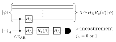
Figure 1: The circuit for implementing the ancilla-driven quantum computation (ADQC). The upper horizontal lines (the lower line) represents register qubits (an ancillary qubit), where $\mbox{\it CZ}_{\mathrm{AR}}$ denotes the controlled-$Z$ gate between one of the register qubits and the ancillary qubit, $H_{\mathrm{R}}$ ($H_{\mathrm{A}}$) denotes the Hadamard gate for the register (ancillary) qubit, and $R_{z}(\beta)$ denotes a parameterized rotation around the $z$-axis with any value $\beta$. We prepare the initial states $\ket{\psi}$ and $\ket{+}_{\mathrm{A}}$ for the register qubits and the ancillary qubit, respectively, where $\ket{\psi}$ denotes an arbitrary input state. After implementing the unitary operation $H_{\mathrm{A}}R_{z}(\beta)E_{\mathrm{AR}}$ and measuring the ancillary qubit in the $z$-basis, where $E_{\mathrm{AR}}\equiv H_{\mathrm{A}}H_{\mathrm{R}}\mbox{\it CZ}_{\mathrm{AR}}$, we obtain $X^{j_{\mathrm{A}}}H_{\mathrm{R}}R_{z}(\beta)\ket{\psi}$ at the register qubits, where $X$ denotes the Pauli-$X$ gate and $j_{\mathrm{A}}=0\ \rm{or}\ 1$ is the result of the measurement.

III Variational quantum algorithm for NISQ device

Variational quantum algorithm (VQAs) perform a required task by preparing a parametrized wave function on a quantum circuit $\ket{\psi(\vec{\theta})}$ with the variational parameters $\vec{\theta}$ to be optimized by minimizing a cost function $C(\vec{\theta})$ tailored to a problem. The parametrized wavefunction can be generally described as $\ket{\psi(\vec{\theta})}=U_{\rm{AN}}(\vec{\theta})\ket{\bar{0}}$ with $\ket{\bar{0}}\equiv\bigotimes_{i=1}^{N}\ket{0}$, where the ansatz quantum circuit is represented as a repetition of parametrized quantum gates and fixed quantum gates as $U_{\rm{AN}}(\vec{\theta})=V_{L+1}U_{L}(\theta_{L})V_{L}U_{L-1}(\theta_{L-1})...U_{1}(\theta_{1})V_{1}$. Here, $L$ is the number of parameters, $U_{k}(\theta_{k})$ and $V_{k}$ are the $k$-th parametrized and fixed gates, respectively, and $\theta_{k}$ is the $k$-th component of the parameter set $\vec{\theta}$. As an example of the cost function, in the celebrated variational quantum eigensolver (VQE) Peruzzo et al. (2014); McClean et al. (2016), one uses the expectation value of the Hamiltonian $H$, i.e., $\bra{\psi(\vec{\theta})}H\ket{\psi(\vec{\theta})}$. Typically, the parameters at $(j+1)$-th step $\vec{\theta}[j+1]$ is obtained by optimizing the cost function at the $j$-th step $C(\vec{\theta}[j])$ by using e.g., gradient descent methods. The total number of iteration steps to update the parameters is defined as $M$. The other example of VQAs is variational quantum simulation (VQS), which is used to simulate quantum dynamics such as Schrödinger equation Li and Benjamin (2017); Yuan et al. (2019). By using the variational principles, it is possible to minimize the distance between the ideal state in the exact evolution and the parametrized trial state, which provides us with the feasible update rule of parameters.

In variational algorithms, we should implement not only the original quantum circuit but also variant types of the original circuit. For example, in many variational algorithms, derivatives of quantum states, i.e., $\frac{\partial\ket{\psi(\vec{\theta})}}{\partial\theta_{k}}$ are used. They are generated from a different quantum circuit from the original ansatz circuit. To discuss these cases in a general form, we denote the set of variational quantum circuits used in the algorithm as $\{U^{(i)}_{\rm{AN}}(\vec{\theta})\}_{i=1}^{G}\equiv\{V^{(i)}_{L+1}U^{(i)}_{L}(\theta_{L})V^{(i)}_{L}U^{(i)}_{L-1}(\theta_{L-1})V^{(i)}_{L-1}\cdots U^{(i)}_{1}(\theta_{1})V^{(i)}_{1}\}_{i=1}^{G}$, where $G$ is the number of variational quantum circuits including the original and variants. Accordingly, we denote the set of the observables measured in these quantum circuits as $\{\hat{A}^{(i)}_{1},\hat{A}^{(i)}_{2},\cdots,\hat{A}^{(i)}_{K^{(i)}}\}_{i=1}^{G}$, where $\hat{A}^{(i)}$ is a Pauli matrix (or an operator made up of tensor products of the Pauli matrices) and $K^{(i)}$ is the number of observables measured in the $i$-th quantum circuits. We will use these notation throughout this paper. We show a prescription about how to implement the conventional variational algorithms with these notation in Appendix B.

IV Variational Secure Cloud Quantum Computing

We explain our protocol of the variational secure cloud quantum computing. Suppose that a client who has the ability to perform only single-qubit measurements hopes to access the NISQ computer of the server in a secure way. The main purpose of our scheme is to hide the information of the ansatz parameters $\vec{\theta}$ set by the client and output of the algorithm. In our scheme, the ansatz circuit to be implemented by the server is publicly announced beforehand. Our scheme is efficient for the NISQ device that has a limited resource, because our scheme requires only a single ancillary qubit independently of the number of qubits needed in the original NISQ algorithm. These are in stark contrast with the original BQC. In the BQC, every information of the choice of the client is hidden Broadbent et al. (2009); Morimae and Fujii (2013a); Takeuchi et al. (2016); Barz et al. (2012); Greganti et al. (2016), while $3N$ qubits are approximately required to execute an algorithm using $N$ qubits.

Throughout our paper, we assume that the client has his/her own private space, and any information in the private space is not leaked to the outside. This is the standard assumption in the quantum key distribution Scarani et al. (2009)

The key of our protocol is to use the concept of the ADQC when the server runs the NISQ computing algorithm. We assume that the server has register qubits, and an ancillary qubit can be sent from the server to the client. When the server needs to implement a single-qubit operation based on the ansatz, the server uses the single-qubit rotation scheme of the ADQC as shown in Fig. 2. More specifically, the server performs a two-qubit gate $E_{\mathrm{AR}}$ between the register qubit (that we want to perform the single-qubit rotation) and the ancillary qubit, and sends the client the ancillary qubit to be measured by the client side. The angle and axis of the single-qubit rotation are determined by the client. With three sets of the rotation, an arbitrary single-qubit rotation can be achieved in a register qubit (see Appendix A).

Moreover, by performing a single-qubit rotation on every register qubit in this way, we have byproduct operators of $X^{j_{1}+j_{3}}Z^{j_{2}}$ on every register qubit as shown in Eq. (1). It is known that, when Pauli matrices or an identity operator are randomly implemented on a quantum state (see Sec. 8.3.4 in Ref. Nielsen and Chuang (2002)), the state becomes completely mixed. This means that the byproduct operators make the state completely mixed for the server. Due to this property, any measurements on the server side provide random outcomes if the server side does not have any information of the client’s dataset, which is helpful for the client to hide the output of the algorithm. The security of our scheme can be also interpreted as follows. During the implementations of these gates in our scheme, the gate operations executed by the server do not depend on the ansatz parameters. Moreover, the client does not send any information to the server during our protocol. Therefore, the server cannot find the parameters of the ansatz circuit set by the client. Such security is guaranteed by the no-signaling principle Popescu and Rohrlich (1994); Morimae and Fujii (2013b).

When the server needs to perform a two-qubit gate based on the ansatz with a specific angle, we adopt a quantum circuit shown in Fig. 3. The point is that an arbitrary two-qubit gate can be decomposed by arbitrary single-qubit gates and controlled-$Z$ gates. We combine the single-qubit rotations in the ADQC with two controlled-$Z$ gates as shown in Fig. 3. In this case, the angles of the two-qubit gates can be determined by the client because the angle of the single-qubit gate can be specified just by the client. Similar to the case of the single-qubit gates, the no-signaling principle guarantees that the server does not obtain any information about the ansatz parameters during the implementation of the two-qubit gates.

The combinations of the single-qubit gates and two-qubit gates in our architecture are shown in Fig. 4. The server performs only Hadamard gates, phase gates, and controlled-$Z$ gates, which are clifford gates. Therefore, when the server measures the observables in the register qubits and sends the measurement results to the client, the client can effectively remove the effect of the byproduct operators by changing the interpretation of the measurement results (see Appendix A).

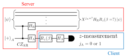
Figure 2: A quantum circuit to implement a single-qubit rotation by the client in our scheme. The circuit is the same as that in Fig. 1. Firstly, the server entangles one register qubit with an ancillary qubit by the unitary operation $E_{\mathrm{AR}}=H_{\mathrm{A}}H_{\mathrm{R}}\mbox{\it CZ}_{\mathrm{AR}}$. Secondly, the server sends the ancillary qubit to the client. Thirdly, the client performs a single-qubit rotation of $H_{\mathrm{A}}R_{z}(\beta)$ on the ancillary qubit, where $\beta$ is determined only by the client. Finally, after the client measures the ancillary qubit in the $z$-basis, $X^{j_{\mathrm{A}}}H_{\mathrm{R}}R_{z}(\beta)\ket{\psi}$ is generated for the register qubit. Since the client does not send any signals to the server, the server does not have any information about the rotation angle $\beta$ and a measurement result $j_{\mathrm{A}}$, which is guaranteed by the no-signaling principle. By repeating this process several times, arbitrary single-qubit rotations on a register qubit can be implemented.

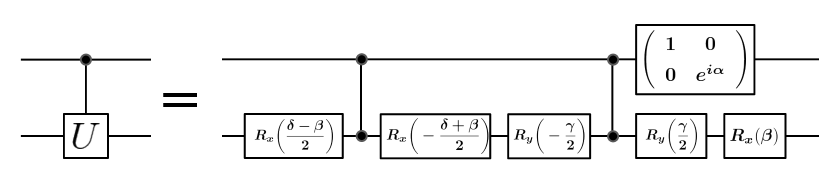
(a)

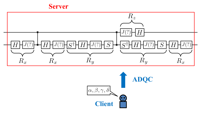
(b)

Figure 3: An implementation of two-qubit gates in our scheme. (a) An equivalent circuit with a controlled-gate operation. We can decompose an arbitrary two-qubit gate into several gates such as single-qubit rotations (including parameters) and controlled-$Z$ gates, where we need to choose appropriate parameters of $\alpha,\beta,\gamma$, and $\delta$ for the equivalence. (b) A quantum circuit to implement an arbitrary controlled-gate operation by the client while the rotation parameters are hidden to the server in our scheme. The basic structure of the circuit is the same as that in (a), where $S$ denotes a phase gate. The Hadamard, the controlled-$Z$, and the phase gates are implemented by the server in the register qubits. An important point is that every single-qubit rotation in the circuit should be performed by the client in the same way as described in Fig. 2. In this case, no-signaling principle guarantees that the rotation parameters ($\alpha$, $\beta$, $\gamma$, and $\delta$) cannot be inferred by any operation on the server.

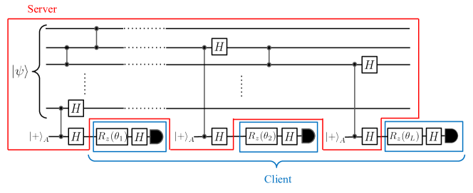
Figure 4: A quantum circuit to implement our variational secure cloud quantum computing. The NISQ algorithm requires the parameters $\{\theta_{j}\}_{j=1}^{L}$ to change the ansatz circuit in a variational way. The server implements gate operations that do not depend on the parameters, and sends the ancillary qubit to the client. On the other hand, the client can specify the parameters by changing the measurement angles on the ancillary qubits sent from the server. Importantly, in our scheme, the client does not send any signal to the server, and thus the server does not know the parameters set by the client, due to the no-signaling principle.

Before the client performs the secure cloud NISQ computation, the server publicly announces the set of unitary operators $\{U^{(i)}_{\rm{AN}}\}_{i=1}^{G}$, the set of the observables $\{\hat{A}^{(i)}_{1},\hat{A}^{(i)}_{2},\cdots,\hat{A}^{(i)}_{K^{(i)}}\}_{i=1}^{G}$, the repetition numbers $\{N^{(i)}\}_{i=1}^{G}$ for sampling with the quantum circuits, initial states $\{\ket{\psi^{(i)}(\vec{\theta}[0])}\}_{i=1}^{G}$, $L$ (the number of variational parameters), $M$ (the total number of iteration steps for VQAs), and $G$ (the number of variants of variational quantum circuits), as shown in Fig. 5.

We summarize our scheme in Fig. 6 as follows.

1. Adopting the quantum circuits of $\{U^{(i)}_{\rm{AN}}\}_{i=1}^{G}$, the server and client implement these unitary operations to generate the trial wave functions $\{\ket{\psi^{(i)}(\vec{\theta}[1])}\}_{i=1}^{G}$. Here, parametrized single- and two-qubit gates should be implemented in the specific ways as described in Figs. 2 and 3, respectively. More specifically, the server performs operations, such as the Hadamard, the controlled-$Z$, and the phase gates (1.a in Fig. 6), while the client specifies the measurement angles (1.b of Fig. 6). We do not need to prepare $\{\ket{\psi^{(i)}(\vec{\theta}[1])}\}_{i=1}^{G}$ simultaneously by using $G$ quantum computers, but we can prepare and measure these in sequence by using a single quantum computer, similar to the standard VQA for NISQ devices (see Appendix B).

2. The server measures the states of the register qubits with $\{\hat{A}^{(i)}_{1},\hat{A}^{(i)}_{2},\cdots,\hat{A}^{(i)}_{K^{(i)}}\}_{i=1}^{G}$, and sends the results to the client with classical communications.

3. For the sampling, the server and client repeat the first and the second steps with $\{N^{(i)}\}_{i=1}^{G}$ times for each state $\{\ket{\psi^{(i)}(\vec{\theta}[1])}\}_{i=1}^{G}$ so that the client should obtain the expectation values of $\{\hat{A}^{(i)}_{1},\hat{A}^{(i)}_{2},\cdots,\hat{A}^{(i)}_{K^{(i)}}\}_{i=1}^{G}$. When the observables are measured, the effect of the byproduct operators can be canceled out by the client (see Appendix A).

4. By processing the measurement results with a classical computer at the client side, the client updates the parameters and obtains $\vec{\theta}[2]=(\theta_{1}[2],\cdots,\theta_{L}[2])^{T}$ for the next step.

5. The client and the server repeat the steps 1-4 $(M-2)$ times with $\{U^{(i)}_{\rm{AN}}\}_{i=1}^{G}$ and $\vec{\theta}[j]$, where classical computation based on the results at the $j$-th step provides the client with the updated parameters of $\vec{\theta}[j+1]$ for $j=2,3,\cdots,M-1$. The client finally obtains desired results in a secure way from the server.

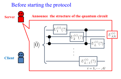
Figure 5: Before the client starts the protocol, the server broadcasts the information about their quantum circuit. This includes the set of unitary operations $\{U^{(i)}_{\rm{AN}}\}_{i=1}^{G}$, the set of the observables $\{\hat{A}^{(i)}_{1},\hat{A}^{(i)}_{2},\cdots,\hat{A}^{(i)}_{K^{(i)}}\}_{i=1}^{G}$ to be measured, the repetition numbers $\{N^{(i)}\}_{i=1}^{G}$ for the quantum circuits, initial states $\{\ket{\psi^{(i)}(\vec{\theta}[0])}\}_{i=1}^{G}$, and the total number $M$ of iteration steps to update the parameters. The client implements the NISQ algorithm based on this information.

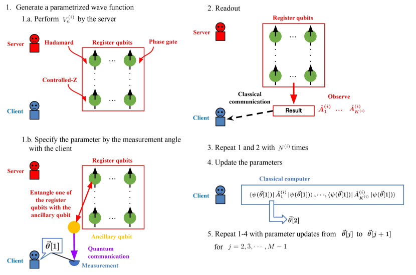
Figure 6: The sequence of our scheme to implement a NISQ algorithm with a parameter set of $\vec{\theta}$ in a variational secure cloud quantum computing. (1) The server sequentially performs the unitary operations $\{U^{(i)}_{\rm{AN}}\}_{i=1}^{G}$ for the register qubits, where $G$ denotes the number of the quantum circuits to be performed. (1.a) The server implements a unitary (non-parameterized) operation $V^{(i)}_{n}$ for $n=1,2,\cdots,L+1$; a Hadamard or a controlled-$Z$, or a phase gate, on the register qubits. (1.b) The server entangles a register qubit with an ancillary qubit and sends the ancillary qubit to the client in the same way as Fig. 2. The client measures the ancillary qubit sent from the server, where the client specifies a measurement angle based on the initial parameters $\vec{\theta}[1]$. (2) The server measures $\hat{A}^{(i)}_{1},\hat{A}^{(i)}_{2},\cdots,$ and $\hat{A}^{(i)}_{K^{(i)}}$ for $i=1,2,\cdots,G$ and sends the results to the client by the classical communication. (3) For each $\{U^{(i)}_{\rm{AN}}\}_{i=1}^{G}$, the server and the client repeat these two steps $\{N^{(i)}\}_{i=1}^{G}$ times, and then the client obtains expectation values of $\{\hat{A}^{(i)}_{1},\hat{A}^{(i)}_{2},\cdots,\hat{A}^{(i)}_{K^{(i)}}\}_{i=1}^{G}$ with $\{\ket{\psi^{(i)}(\vec{\theta}[1])}\}_{i=1}^{G}$. (4) The client updates the parameters as $\vec{\theta}[2]$ by processing the measurement data with classical computation. (5) The server and the client repeat these four steps with $M-2$ times updating the parameters from $\vec{\theta}[j]$ to $\vec{\theta}[j+1]$ for $j=2,3,\cdots,M-1$, and the client obtains the output. Since the client does not send any signals to the server during the computation, the server cannot obtain any information about $\vec{\theta}[1]$, $\vec{\theta}[2]$, $\dots$, $\vec{\theta}[M]$, because of the no-signaling principle.

As a physical implementation, the register qubits can be the solid-state systems that interact with a photon, and the ancillary qubit can be an optical photon that transmits to a distant place. We implicitly assumed that the photon loss would be negligible during the transmission in the discussion above.

Finally, we discuss the effect of photon loss on our scheme. When the server sends the client an ancillary qubit that corresponds to an optical photon, there is a possibility that the photon can be lost during the transmission. In principle, if the server and the client have quantum memories, they can share a Bell pair under the effect of photon loss by repeating the entanglement generation process until success Benjamin et al. (2006), and they can use the Bell pairs to perform our gate operations in a deterministic way. In this case, the client needs to ask the server to send the photons again and again, depending on how many times the photon is lost Benjamin et al. (2006). However, in order to apply the no-signaling principle, the client is not allowed to send the server any information. This means that the client cannot ask the server to send the photon again. So we cannot adopt the repeat-until-success strategy with quantum memories.

Thus, we assume that the client adopts the observation results of the readout of the register qubits by the server only when all photons are successfully transmitted to the client during the computation. In this case, the probability of the no photon loss during the computation exponentially decreases as the number of sending photons increases. The number of required photons sent to the client can be determined by the number of the tunable parameters used in the ansatz circuit. When $U^{(i)}_{\mathrm{AN}}$ is composed of $n^{(i)}_{\rm{single}}$ single-qubit operations and $n^{(i)}_{\rm{two}}=L-n^{(i)}_{\rm{single}}$ two-qubit operations, the necessary number $N_{\rm{ph}}^{(i)}$ of the photons to send the client is at most $N^{(i)}_{\rm{ph}}=3n^{(i)}_{\rm{single}}+6n^{(i)}_{\rm{two}}$ as shown in Eq. 1 and Figs. 2 and 3. The probability for all the photons to be detected by the client is $(1-p_{\rm{loss}})^{N_{\rm{ph}}^{(i)}}$, where $p_{\rm{loss}}$ is a photon loss probability for a single transmission. Therefore, the repetition number $N^{(i)}$ with the photon loss should be set to be much larger than $N_{\rm{ideal}}^{(i)}/(1-p_{\rm{loss}})^{N_{\rm{ph}}^{(i)}}$, where $N_{\rm{ideal}}^{(i)}$ denotes the required number of repetition with no photon loss. To keep $N^{(i)}$ within a reasonable amount, $p_{\rm{loss}}$ should be smaller than $1\%$ under the assumption that $N_{\rm{ph}}^{(i)}$ is around a few hundreds.

We could overcome such a problem due to the recent experimental and theoretical developments of quantum repeating technology. The best single-photon detector in optics has $99\%$ efficiency Lita et al. (2010); Fukuda et al. (2011); Kuzanyan et al. (2018). Microwave quantum repeater with a short distance such as 100 m has been proposed Xiang et al. (2017), and a qubit can catch a microwave photon with $99.4\%$ absorption efficiency in the microwave regime Wenner et al. (2014). Also, there are proposals to physically move the solid-state qubit Schaffry et al. (2011); Devitt et al. (2016) for distributed quantum computation or a quantum repeater Through the combination of these protocols and a long-lived quantum memory such as a nuclear spin Saeedi et al. (2013); Aslam et al. (2017), the ancillary solid-state qubits might be carried to the client without the problems of the photon loss.

V Conclusion

In conclusion, we proposed a noisy intermediate-scale quantum (NISQ) computing with security inbuilt. The main targets of our scheme are variational quantum algorithms (VQAs), which involve parameters of an ansatz to be optimized by minimizing a cost function. We considered a circumstance that a client with a limited ability to perform quantum operations hopes to access a NISQ device possessed by a server and the client tries to avoid leakage of the information about the quantum algorithm that he/she runs. Importantly, the naive application of the previously known blind quantum computation (BQC) Morimae and Fujii (2013b) requires around $3N$ qubits Raussendorf and Briegel (2001); Raussendorf et al. (2003); Walther et al. (2005), where $N$ denotes the number of the qubits to run the quantum algorithm in the original architecture. That may not be suitable for the NISQ devices with the limited number of qubits. Our proposal is more efficient in the sense that we use a single ancillary qubit and $N$ register qubits required in the original NISQ algorithm. In VQAs, we use a parametrized trial wave function, and our scheme prevents the information about the parameters from the leakage to the server. We rely on the no-signaling principle to guarantee security. Our scheme paves the way for new applications of the NISQ devices.

Y. S. and Y. T. contributed to this work equally. This work was supported by Leading Initiative for Excellent Young Researchers MEXT Japan and JST presto (Grant No. JPMJPR1919) Japan. This work was supported by MEXT Quantum Leap Flagship Program (MEXT Q-LEAP) (Grant No. JPMXS0120319794, JPMXS0118068682), JST ERATO (Grant No. JPMJER1601), JST [Moonshot R&D–MILLENNIA Program] Grant No. JPMJMS2061, MEXT Quantum Leap Flagship Program (MEXT Q-LEAP) Grant No. JPMXS0118067394, and S.W. was supported by Nanotech CUPAL,National Institute of Advanced Industrial Science and Technology (AIST). This paper was partly based on results obtained from a project, JPNP16007, commissioned by the New Energy and Industrial Technology Development Organization (NEDO), Japan.

Appendix A Detailed ancilla-driven quantum computation

A.1 Arbitrary single-qubit rotation

We describe a way to implement an arbitrary single-qubit rotation. Any single-qubit rotation $U$ can be represented by $U=R_{z}(\beta^{\prime})R_{x}(\gamma^{\prime})R_{z}(\delta^{\prime})$, where $R_{x}$ denotes a rotation about the $x$-axis, and $\beta^{\prime}$, $\gamma^{\prime}$, and $\delta^{\prime}$ denote the rotation angles about the corresponding axis. Defining $J(\beta)\equiv HR_{z}(\beta)$, one can rewrite $U$ as $U=J(\beta)J(\gamma)J(\delta)$, where we choose $\beta$, $\gamma$, and $\delta$ to satisfy $R_{z}(\beta)R_{x}(\gamma)R_{z}(\delta)=HU$. As we explained, one can implement the single-qubit rotation of $X^{j}H_{\mathrm{R}}R_{z}(\beta)\ket{\psi}$ on the register qubit by the coupling with an ancillary qubit and a subsequent measurement. Therefore, three sequential operations of this type of the single-qubit rotation provide us with the following operation

$$\Big{(}X^{j_{3}}H_{\mathrm{R}}R_{z}((-1)^{j_{2}}\beta)\Big{)}\Big{(}X^{j_{2}}H_{\mathrm{R}}R_{z}((-1)^{j_{1}}\gamma)\Big{)}\Big{(}X^{j_{1}}H_{\mathrm{R}}R_{z}(\delta)\Big{)}$$ (1)

$$= X^{j_{3}}J((-1)^{j_{2}}\beta)X^{j_{2}}J((-1)^{j_{1}}\gamma)X^{j_{1}}J(\delta)$$

$$= (-1)^{j_{1}\cdot j_{2}}X^{j_{1}+j_{3}}Z^{j_{2}}J(\beta)J(\gamma)J(\delta)$$

where $j_{i}$ denotes the result of the $i$-th measurement on the ancillary qubits. For the implementation of this operation, we change the rotation angle of the ancillary qubit depending on the previous measurement results. Equation. (1) involves the byproduct operator $X^{j_{1}+j_{3}}Z^{j_{2}}$. However, as long as we measure the qubit in a computational basis for the readout, the byproduct operators just flip the measurement result from $0$ to $1$ or vice versa, and so we can effectively remove the byproduct operators from the states by changing the interpretation of the measurement results.

A.2 Two-qubit gate between the register qubits

We explain a way to perform the controlled-$Z$ gate on the two register qubits $R$ and $R^{\prime}$ in the ADQC. Firstly, we implement $E_{\mathrm{AR}}$ on the ancillary qubit (prepared in the state $\ket{+}_{\mathrm{A}}$) and the register qubit $R$, and subsequently perform $E_{\mathrm{AR^{\prime}}}$ on the ancillary qubit and the other register qubit $R^{\prime}$. Secondly, one measures the ancillary qubit in the y-basis. These operations are equivalent to the controlled-$Z$ gate, up to local operations. When we perform several single-qubit gates and two-qubit gates, the byproduct operators are applied as $U_{\Sigma}U_{\rm{ideal}}|\overline{0}\rangle$, where $U_{\Sigma}$ denotes the total byproduct operators and $U_{\rm{ideal}}$ denotes the unitary operations that we aim to implement. Again, when one measures observables of Pauli matrices (or a tensor product of Pauli matrices), one can effectively remove the byproduct operators from the states by changing the interpretation of the measurement results.

Appendix B VQA for NISQ devices

We show a prescription about how to implement the conventional variational algorithms with our notation. We prepare a parametrized wave function on a quantum circuit $\ket{\psi(\vec{\theta})}$ with the variational parameters $\vec{\theta}$ to be optimized by minimizing a cost function $C(\vec{\theta})$ tailored to a problem. Firstly, with the quantum circuits of $\{U^{(i)}_{\rm{AN}}\}_{i=1}^{G}$, we realize parametrized wave functions of $N$-qubits $\{\ket{\psi^{(i)}(\vec{\theta}[1])}\}_{i=1}^{G}$, where $\ket{\psi^{(i)}(\vec{\theta}[1])}\equiv V^{(i)}_{L+1}U^{(i)}_{L}(\theta_{L}[1])V^{(i)}_{L}\cdots U^{(i)}_{1}(\theta_{1}[1])V^{(i)}_{1}\ket{\bar{0}}$ with $\ket{\bar{0}}\equiv\bigotimes_{i=1}^{N}\ket{0}$ denotes the wave function, $\vec{\theta}[1]=(\theta_{1}[1],\cdots,\theta_{L}[1])^{T}$ is a vector of the parameters and $\{\ket{\psi^{(i)}(\vec{\theta}[0])}\}_{i=1}^{G}$ are initial states, and we measure the state of the wave function with observables of $\{\hat{A}^{(i)}_{1}$, $\hat{A}^{(i)}_{2}$, $\cdots$, $\hat{A}^{(i)}_{K^{(i)}}\}_{i=1}^{G}$.

Secondly, for the sampling, we repeat the first step to obtain expectation values of $\{\hat{A}^{(i)}_{1},\hat{A}^{(i)}_{2},\cdots,\hat{A}^{(i)}_{K^{(i)}}\}_{i=1}^{G}$ with $\{\ket{\psi^{(i)}(\vec{\theta}[1])}\}_{i=1}^{G}$. Thirdly, based on the expectation values, we implement a classical algorithm so that we can obtain updated parameters $\vec{\theta}[2]$ for the next quantum circuits, where we typically use a gradient method to make the cost function smaller. For example, we use $\vec{\theta}[j+1]=\vec{\theta}[j]-\alpha{\rm{grad}}C(\vec{\theta}[j])$ for the gradient method.

Finally, we repeat the first, second, and third steps $M-2$ times with $\{U^{(i)}_{\rm{AN}}\}_{i=1}^{G}$ and $\vec{\theta}[k]$, where classical computation based on the results at the $k$-th step provides the updated parameters of $\vec{\theta}[k+1]$ for $k=2,3,\cdots,M-1$. These processes provide us with an output of the algorithm.

References

- Shor (1997) P. W. Shor, SIAM Journal on Computing 26, 1484 (1997), https://doi.org/10.1137/S0097539795293172 .
- Grover (1997) L. K. Grover, Physical review letters 79, 325 (1997).
- Harrow et al. (2009) A. W. Harrow, A. Hassidim, and S. Lloyd, Physical review letters 103, 150502 (2009).
- Vandersypen et al. (2001) L. M. Vandersypen, M. Steffen, G. Breyta, C. S. Yannoni, M. H. Sherwood, and I. L. Chuang, Nature 414, 883 (2001).
- Bennett and Brassard (1984) C. H. Bennett and G. Brassard, “Proceedings of the ieee international conference on computers, systems and signal processing,” (1984).
- Bennett et al. (1992) C. H. Bennett, F. Bessette, G. Brassard, L. Salvail, and J. Smolin, Journal of cryptology 5, 3 (1992).
- Gisin et al. (2002) N. Gisin, G. Ribordy, W. Tittel, and H. Zbinden, Rev. Mod. Phys. 74, 145 (2002).
- Broadbent et al. (2009) A. Broadbent, J. Fitzsimons, and E. Kashefi, in 2009 50th Annual IEEE Symposium on Foundations of Computer Science (2009) pp. 517–526.
- Dowling and Milburn (2003) J. P. Dowling and G. J. Milburn, Philosophical Transactions of the Royal Society of London. Series A: Mathematical, Physical and Engineering Sciences 361, 1655 (2003).
- Spiller et al. (2005) T. P. Spiller, W. J. Munro, S. D. Barrett, and P. Kok, Contemporary Physics 46, 407 (2005), https://doi.org/10.1080/00107510500293261 .
- Degen et al. (2017) C. L. Degen, F. Reinhard, and P. Cappellaro, Rev. Mod. Phys. 89, 035002 (2017).
- Budker and Romalis (2007) D. Budker and M. Romalis, Nature physics 3, 227 (2007).
- Balasubramanian et al. (2008) G. Balasubramanian, I. Chan, R. Kolesov, M. Al-Hmoud, J. Tisler, C. Shin, C. Kim, A. Wojcik, P. R. Hemmer, A. Krueger, et al., Nature 455, 648 (2008).
- Maze et al. (2008) J. R. Maze, P. L. Stanwix, J. S. Hodges, S. Hong, J. M. Taylor, P. Cappellaro, L. Jiang, M. G. Dutt, E. Togan, A. Zibrov, et al., Nature 455, 644 (2008).
- Neumann et al. (2013) P. Neumann, I. Jakobi, F. Dolde, C. Burk, R. Reuter, G. Waldherr, J. Honert, T. Wolf, A. Brunner, J. H. Shim, et al., Nano letters 13, 2738 (2013).
- Wineland et al. (1992) D. J. Wineland, J. J. Bollinger, W. M. Itano, F. Moore, and D. Heinzen, Physical Review A 46, R6797 (1992).
- Huelga et al. (1997) S. F. Huelga, C. Macchiavello, T. Pellizzari, A. K. Ekert, M. B. Plenio, and J. I. Cirac, Physical Review Letters 79, 3865 (1997).
- Matsuzaki et al. (2011) Y. Matsuzaki, S. C. Benjamin, and J. Fitzsimons, Physical Review A 84, 012103 (2011).
- Chin et al. (2012) A. W. Chin, S. F. Huelga, and M. B. Plenio, Physical review letters 109, 233601 (2012).
- Kessler et al. (2014) E. M. Kessler, I. Lovchinsky, A. O. Sushkov, and M. D. Lukin, Physical review letters 112, 150802 (2014).
- Dür et al. (2014) W. Dür, M. Skotiniotis, F. Froewis, and B. Kraus, Physical Review Letters 112, 080801 (2014).
- Arrad et al. (2014) G. Arrad, Y. Vinkler, D. Aharonov, and A. Retzker, Physical review letters 112, 150801 (2014).
- Herrera-Martí et al. (2015) D. A. Herrera-Martí, T. Gefen, D. Aharonov, N. Katz, and A. Retzker, Physical review letters 115, 200501 (2015).
- Unden et al. (2016) T. Unden, P. Balasubramanian, D. Louzon, Y. Vinkler, M. B. Plenio, M. Markham, D. Twitchen, A. Stacey, I. Lovchinsky, A. O. Sushkov, et al., Physical review letters 116, 230502 (2016).
- Matsuzaki and Benjamin (2017) Y. Matsuzaki and S. Benjamin, Physical Review A 95, 032303 (2017).
- Higgins et al. (2007) B. L. Higgins, D. W. Berry, S. D. Bartlett, H. M. Wiseman, and G. J. Pryde, Nature 450, 393 (2007).
- Waldherr et al. (2012) G. Waldherr, J. Beck, P. Neumann, R. Said, M. Nitsche, M. Markham, D. Twitchen, J. Twamley, F. Jelezko, and J. Wrachtrup, Nature nanotechnology 7, 105 (2012).
- Komar et al. (2014) P. Komar, E. M. Kessler, M. Bishof, L. Jiang, A. S. Sørensen, J. Ye, and M. D. Lukin, Nature Physics 10, 582 (2014).
- Proctor et al. (2018) T. J. Proctor, P. A. Knott, and J. A. Dunningham, Physical review letters 120, 080501 (2018).
- Eldredge et al. (2018) Z. Eldredge, M. Foss-Feig, J. A. Gross, S. L. Rolston, and A. V. Gorshkov, Physical Review A 97, 042337 (2018).
- Giovannetti et al. (2002a) V. Giovannetti, S. Lloyd, and L. Maccone, Journal of Optics B: Quantum and Semiclassical Optics 4, S413 (2002a).
- Giovannetti et al. (2002b) V. Giovannetti, S. Lloyd, and L. Maccone, Physical Review A 65, 022309 (2002b).
- Chiribella et al. (2007) G. Chiribella, L. Maccone, and P. Perinotti, Physical review letters 98, 120501 (2007).
- Huang et al. (2019) Z. Huang, C. Macchiavello, and L. Maccone, Physical Review A 99, 022314 (2019).
- Takeuchi et al. (2019) Y. Takeuchi, Y. Matsuzaki, K. Miyanishi, T. Sugiyama, and W. J. Munro, Physical Review A 99, 022325 (2019).
- Yin et al. (2020) P. Yin, Y. Takeuchi, W.-H. Zhang, Z.-Q. Yin, Y. Matsuzaki, X.-X. Peng, X.-Y. Xu, J.-S. Xu, J.-S. Tang, Z.-Q. Zhou, et al., Physical Review Applied 14, 014065 (2020).
- Broadbent et al. (2009) A. Broadbent, J. Fitzsimons, and E. Kashefi, in 2009 50th Annual IEEE Symposium on Foundations of Computer Science (IEEE, 2009) pp. 517–526.
- Morimae and Fujii (2013a) T. Morimae and K. Fujii, Phys. Rev. A 87, 050301 (2013a).
- Takeuchi et al. (2016) Y. Takeuchi, K. Fujii, R. Ikuta, T. Yamamoto, and N. Imoto, Phys. Rev. A 93, 052307 (2016).
- Barz et al. (2012) S. Barz, E. Kashefi, A. Broadbent, J. F. Fitzsimons, A. Zeilinger, and P. Walther, Science 335, 303 (2012), https://science.sciencemag.org/content/335/6066/303.full.pdf .
- Greganti et al. (2016) C. Greganti, M.-C. Roehsner, S. Barz, T. Morimae, and P. Walther, New Journal of Physics 18, 013020 (2016).
- Raussendorf and Briegel (2001) R. Raussendorf and H. J. Briegel, Physical Review Letters 86, 5188 (2001).
- Raussendorf et al. (2003) R. Raussendorf, D. E. Browne, and H. J. Briegel, Physical review A 68, 022312 (2003).
- Walther et al. (2005) P. Walther, K. J. Resch, T. Rudolph, E. Schenck, H. Weinfurter, V. Vedral, M. Aspelmeyer, and A. Zeilinger, Nature 434, 169 (2005).
- Popescu and Rohrlich (1994) S. Popescu and D. Rohrlich, Foundations of Physics 24, 379 (1994).
- Morimae and Fujii (2013b) T. Morimae and K. Fujii, Physical Review A 87, 050301 (2013b).
- Endo et al. (2021) S. Endo, Z. Cai, S. C. Benjamin, and X. Yuan, Journal of the Physical Society of Japan 90, 032001 (2021).
- Peruzzo et al. (2014) A. Peruzzo, J. McClean, P. Shadbolt, M.-H. Yung, X.-Q. Zhou, P. J. Love, A. Aspuru-Guzik, and J. L. O’brien, Nature communications 5, 1 (2014).
- Kandala et al. (2017) A. Kandala, A. Mezzacapo, K. Temme, M. Takita, M. Brink, J. M. Chow, and J. M. Gambetta, Nature 549, 242 (2017).
- Moll et al. (2018) N. Moll, P. Barkoutsos, L. S. Bishop, J. M. Chow, A. Cross, D. J. Egger, S. Filipp, A. Fuhrer, J. M. Gambetta, M. Ganzhorn, et al., Quantum Science and Technology 3, 030503 (2018).
- McClean et al. (2016) J. R. McClean, J. Romero, R. Babbush, and A. Aspuru-Guzik, New Journal of Physics 18, 023023 (2016).
- Farhi et al. (2014) E. Farhi, J. Goldstone, and S. Gutmann, arXiv preprint arXiv:1411.4028 (2014).
- Li and Benjamin (2017) Y. Li and S. C. Benjamin, Physical Review X 7, 021050 (2017).
- Yuan et al. (2019) X. Yuan, S. Endo, Q. Zhao, Y. Li, and S. C. Benjamin, Quantum 3, 191 (2019).
- Mitarai et al. (2018) K. Mitarai, M. Negoro, M. Kitagawa, and K. Fujii, Physical Review A 98, 032309 (2018).
- Schuld et al. (2020) M. Schuld, A. Bocharov, K. M. Svore, and N. Wiebe, Physical Review A 101, 032308 (2020).
- Farhi et al. (2020) E. Farhi, H. Neven, et al., Quantum Review Letters 1, 10 (2020).
- Zoufal et al. (2021) C. Zoufal, A. Lucchi, and S. Woerner, Quantum Machine Intelligence 3, 1 (2021).
- Shingu et al. (2020) Y. Shingu, Y. Seki, S. Watabe, S. Endo, Y. Matsuzaki, S. Kawabata, T. Nikuni, and H. Hakoshima, arXiv preprint arXiv:2007.00876 (2020).
- Anders et al. (2010) J. Anders, D. K. Oi, E. Kashefi, D. E. Browne, and E. Andersson, Physical Review A 82, 020301 (2010).
- Bocharov et al. (2015) A. Bocharov, M. Roetteler, and K. M. Svore, Physical review letters 114, 080502 (2015).
- Browne and Briegel (2016) D. Browne and H. Briegel, Quantum Information: From Foundations to Quantum Technology Applications , 449 (2016).
- Paetznick and Svore (2013) A. Paetznick and K. M. Svore, arXiv preprint arXiv:1311.1074 (2013).
- Scarani et al. (2009) V. Scarani, H. Bechmann-Pasquinucci, N. J. Cerf, M. Dušek, N. Lütkenhaus, and M. Peev, Reviews of modern physics 81, 1301 (2009).
- Nielsen and Chuang (2002) M. A. Nielsen and I. Chuang, “Quantum computation and quantum information,” (2002).
- Benjamin et al. (2006) S. C. Benjamin, D. E. Browne, J. Fitzsimons, and J. J. Morton, New Journal of Physics 8, 141 (2006).
- Lita et al. (2010) A. E. Lita, B. Calkins, L. Pellouchoud, A. J. Miller, and S. Nam, in Advanced Photon Counting Techniques IV, Vol. 7681 (International Society for Optics and Photonics, 2010) p. 76810D.
- Fukuda et al. (2011) D. Fukuda, G. Fujii, T. Numata, K. Amemiya, A. Yoshizawa, H. Tsuchida, H. Fujino, H. Ishii, T. Itatani, S. Inoue, et al., Optics express 19, 870 (2011).
- Kuzanyan et al. (2018) A. Kuzanyan, A. Kuzanyan, and V. Nikoghosyan, Journal of Contemporary Physics (Armenian Academy of Sciences) 53, 338 (2018).
- Xiang et al. (2017) Z.-L. Xiang, M. Zhang, L. Jiang, and P. Rabl, Physical Review X 7, 011035 (2017).
- Wenner et al. (2014) J. Wenner, Y. Yin, Y. Chen, R. Barends, B. Chiaro, E. Jeffrey, J. Kelly, A. Megrant, J. Mutus, C. Neill, et al., Physical Review Letters 112, 210501 (2014).
- Schaffry et al. (2011) M. Schaffry, E. M. Gauger, J. J. Morton, and S. C. Benjamin, Physical review letters 107, 207210 (2011).
- Devitt et al. (2016) S. J. Devitt, A. D. Greentree, A. M. Stephens, and R. Van Meter, Scientific reports 6, 1 (2016).
- Saeedi et al. (2013) K. Saeedi, S. Simmons, J. Z. Salvail, P. Dluhy, H. Riemann, N. V. Abrosimov, P. Becker, H.-J. Pohl, J. J. Morton, and M. L. Thewalt, Science 342, 830 (2013).
- Aslam et al. (2017) N. Aslam, M. Pfender, P. Neumann, R. Reuter, A. Zappe, F. F. de Oliveira, A. Denisenko, H. Sumiya, S. Onoda, J. Isoya, et al., Science 357, 67 (2017).