Abstract

Procedural fairness has been a public concern, which leads to controversy when making decisions with respect to protected classes, such as race, social status and disability. Some protected classes can be inferred according to some safe proxies like surname and geolocation for race. Hence, implicitly utilizing the predicted protected classes based on the related proxies when making decisions is an efficient approach to circumvent this issue and seek just decisions. In this article, we propose a hierarchical random forest model for prediction without explicitly involving protected classes. Simulation experiments are conducted to show the performance of hierarchical random forest model. An example is analyzed from Boston police interview records to illustrate the usefulness of the proposed model.

capbtabboxtable[][]

1 Introduction

The United States is one of the most ethnic diverse countries in the world. Thus any unfair decisions regarding protected classes including race and ethnicity can result into huge controversial debate. For example, Larson et al. (2016) questioned the racial fairness of the algorithm: Correctional Offender Management Profiling for Alternative Sanctions (COMPAS), which is a case management and decision support tool used by U.S. courts to assess the likelihood of a defendant becoming a recidivist. Larson et al. (2016) found that blacks are almost twice as likely as whites to be labeled a higher risk but not actually re-offend.

On the other hand, the U.S. Commission on Civil Rights banned police stations to ”redlining” suspects based on certain racial groups, e.g., unreasonable traffic stop on civilians due to factors which show the discrimination to certain civil groups. Therefore, any statistical prediction based on racial profile would also be controversial. Consequently, many surveys or records have eliminated the collection of racial information. However, characteristics such as race, age, and socio-economic class determine other features about us that are relevant to the outcome of some performance tasks. These are protected attributes, but they are still critical to certain tasks.

To resolve this issue, a variety of methods have been proposed. For instance, Chen et al. (2019) employed safe proxies to impute these missing protected variables for statistical prediction. Motivated by this idea, this article proposes a hierarchical random forest to make uncontroversial prediction without explicitly involving protected classes. In the bottom layer of random forest, we adopt proxy variables to predict the protected classes and in the top layer we make the ultimate prediction based on the predicted protected classes along with other factors. We also provide the prediction interval follow the spirit of Meinshausen (2006). Results are found that hierarchical random forest perform even better in some aspects compared to the naive random forest using protected classes directly.

The rest of the paper is organized as follows. In section 2, we introduce the model and prediction interval. Simulations are conducted to validate our model in Section 3. Section 4 elucidate the usefulness of our model by analyzing Boston police interview data. Concluding remarks are present in Section 5

2 Methodology

2.1 Model

Random forests are non-parametric and often accurate and robust to explore a variety of data. Moreover, random forest has been propose for missing data imputation (e.g., see Stekhoven 2015). Thus, we chose random forest to capture the relation between protected classes and other covariates. Our proposed model can be written as

$$\hat{Y}^{(1)}=\hat{f}^{(1)}(\cdot,\hat{Y}^{(2)}),$$

$$\hat{Y}^{(2)}=\hat{f}^{(2)}(\cdot).$$

where $\hat{f}^{(1)}(\cdot)$ and $\hat{f}^{(2)}(\cdot)$ refers to the top and bottom layer random forest methods and $\cdot$ and $\hat{Y}^{(2)}$ refers to the covariates. In our case $\hat{Y}^{(1)}$ refers to the desired predicted result and $\cdot$ refers to the covariates except protected classes such as location and date etc. $\hat{Y}^{(2)}$ refers to the predicted protected classes. In this model, we treat protected classes as latent. As a result, protected classes like race does not explicitly show as covariates. For random forest’s the number of predictors $m$, we consider the number of drawn candidate variables in each split equals to $\sqrt{p}$. Also, we consider the case where the drawn observations are with replacement.Moreover, the node size parameter specifies the minimum number of observations in a terminal node. Setting it lower leads to trees with a larger depth which means that more splits are performed until the terminal nodes. Since we have a large sample size, we would set a larger node size to decrease the computational burden. We employ the algorithm proposed by Breiman (2001) to optimise the model in this article.

2.2 Prediction Interval

The uncertainty of the random forest predictions can be estimated using several approaches including U-statistics approach of Mentch and Hooker (2016) and monte carlo simulations approach of Coulston et al. (2016). Prediction intervals in this paper are constructed by Quantile Regression Forests (Meinshausen 2006). The prediction of random forests can then be seen as an adaptive neighborhood classification and regression procedure (Lin and Jeon 2006). For every covariate, a set of weights for the original observations is obtained. It is illustrated that that random forest not only a good approximation to the conditional mean but to the full conditional distribution. The prediction of random forests is equivalent to the weighted mean of the observed response variables. For quantile regression forests, trees are grown as in the standard random forests algorithm. The conditional distribution is then estimated by the weighted distribution of observed response variables. We only have a brief introduction to Quantile Regression Forests in this article; see Meinshausen (2006) for a more thorough treatment.

3 Simulation Studies

3.1 Simulation Design

To evaluate the performance of the proposed model, we conduct Monte Carlo simulation studies with various settings. We follow Zhu et al. (2015)’s work to create three simulation scenarios that represent different aspects, which usually arise in machine learning. Such aspects include, classification problem and nonlinear structure. For each scenario, we further consider generate independent test samples to calculate the performance measure. Each simulation is repeated $B=100$ times, and the averaged performance is presented. The simulation settings are as follows: We simulated $N$ observations of Normal distribution. Specifically,the simulation settings are as follows: $x_{1}$ and $x_{2}$ are independently generated from uniform distribution $\mathcal{U}\left(0,1\right)$, where $x_{3}$ is computed regarding to $0.4*x_{1}+0.4*x_{2}+0.2*\mathcal{U}\left(0,1\right)$.

Scenario 1: Linear. $Y=3x_{1}+3x_{2}+2x_{3}+\varepsilon$, where $(\cdot)^{+}$ represents the positive part

Scenario 2: Non-Linear. $Y=100(x_{1}-0.5)^{2}(X_{2}-0.25)^{+}+cos(x_{3})+\varepsilon$, where $(\cdot)^{+}$ represents the positive part.

Scenario 3: Classification. Let $\mu=\Phi\left(10\times(x_{1}-1)+10\times|x_{2}-0.5|+10*x_{3}\right),$ where $\Phi$ denotes a normal c.d.f. Draw $Y$ independently from Bernoulli($\mu$).

The above model settings satisfy our technical conditions. For each of the above settings, a total of $N=500$ samples are used.

3.2 Performance Measurement

For a convincing evaluation, we take several measures for comparison. We present the bias $\frac{\sum_{i=1}^{N}\hat{Y}_{i}-Y_{i}}{N}$, standard deviation $\frac{\sqrt{\sum_{i=1}^{N}\left(\hat{Y}_{i}-\frac{\sum_{i=1}^{N}\hat{Y}_{i}}{N}\right)^{2}}}{N}$ and mean square error (MSE) $\frac{\sum_{i=1}^{N}(\hat{Y}_{i}-Y_{i})^{2}}{N}$ for numerical results and confusion matrix for categorical results respectively. For each replication, we obtain $\textrm{bia}_{b},\textrm{\mbox{SD}}_{b},\textrm{MSE}_{b}$ for $b=1,\ldots,B$ and report the average of them.

3.3 Simulation Results

Table 2-4 summarize testing sample prediction error for each simulation setting. We compare the proposed model (with proxy) with naive random forest (without proxy) using protected classes directly. There is clear evidence that the hierarchical random forest produce a reasonable prediction under these settings. For linear settings, the proposed random forest even outperforms naive random forest in terms of bias and standard deviation. This could be caused by the fact that hierarchical random forest correct its predecessor as boosting. The corresponding visualized predicted pattern are shown in Figure 6-8. The black dots are the observed data, lines are predictions and ribbons are the corresponding 90% prediction interval. As we can see that the prediction standard deviation of both models for Non-Linear settings are larger. Overall, two models’ performance are comparable.

	without proxy	with proxy
bias	-0.0043	0.0353
SD	1.5504	1.5263
MSE	5.8402	5.7654

Figure 1: Linear

	without proxy	with proxy
bias	0.0052	0.0064
SD	0.4732	0.5031
MSE	1.3412	1.3749

Figure 2: Non-Linear

	Actual P.	Actual N.
Predicted P.	94.63%	9.64%
Predicted N.	5.36%	90.35%

Figure 3: Confusion matrix without proxy

	Actual P.	Actual N.
Predicted P.	93.77%	10.13%
Predicted N.	6.22%	89.86%

Figure 4: Confusion matrix with proxy

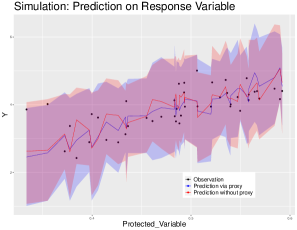
Figure 5: Prediction of Protected Class

Figure 6: Linear

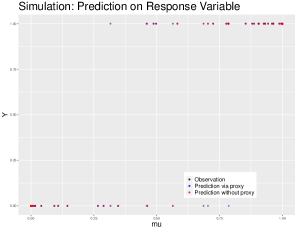
Figure 7: Non-Linear

Figure 8: Classification

4 Real Data Analysis

4.1 Problem Setup

We first present an overview of our dataset. Police field interview data in Boston include 34 variables such as Location, Subject Race, Sex, Reason, Clothing, Vehicle and Officer Race etc. Those data were collected from January 2001 to January 2020 and stored in a 155230 $\times$ 34 data matrix. In our analysis, we use the 10 major variables which includes Sex, Location: Street, Location: District, Location: City, Incident Date, Priors, Race, Skin Complexion, Clothing, Incident Reason . Among these covariates, Race is considered as the protected class in our analysis. As a result, our main objectives are to (1) predict racial profile with a set of factors by bottom-level random forest, (2) predict Incident Reason with predicted latent Race and (3) predict the daily occurrence of police field interview with predicted latent Race Therefore, the racial profile would not be an explicit covariate. We also will compare the prediction accuracy of the hierarchical model with the naive one and discuss the fairness of both models.

4.2 Preliminary Analysis

We have 233 levels for Incident Reasons among 155230 observations. Hence, predicting among 233 levels can have problems such as overfitting. To solve this, we could use cluster method to reduce the dimensions of Incident Reason. The cluster method is reasonable for such work because most of Incident Reason are compounding and similar. For example, one person can be interviewed about Shoplift and another interview is about Theft or Larceny. Those crime would contribute three levels in the original Incident Reason, however, those three are highly related. Moreover, Incident Reason are in the format of text. Some semantic methods have been implemented, however most of them are limited to certain area. Consequently, we decided to use hierarchical Soundex clustering method to group those 233 levels of reasons with Jaro–Winkler distance (see Jaro 1989; Winkler 1990). Soundex is a phonetic algorithm used by the National Archives for indexing names by sound, as pronounced in English. The optimal number of clusters is determined by Elbow method (e.g., see Thorndike 1953). See Van der Loo (2014) for more details about keyword clustering. Finally, we have reduce the dimension of Incident Reason into 6 clusters. The following is the clustering results.

	Related Crime
1	Assault and Battery
2	Violation of Auto Law
3	Larceny, Thief and Vandalism
4	Drug, Narcotics and Alcohol
5	Homicide, Suicide and Deadly Firearms
6	Others such as Harassment and Protective Order

Figure 9: Crime Category Interpretation

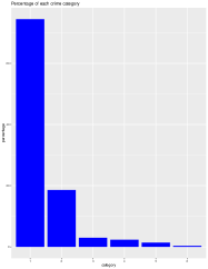
Figure 10: Crime Dendrogram

Figure 11: Percentage of Each Crime Category

Note that we also cluster the Clothing detail in the original data because it was over 10000 levels among 155230 observations. We reduce this levels to 10 clusters as we did for Incident reason. Further preliminary analysis are conducted to show that occurrence of police interview are spatially and temporally correlated. We can clearly see seasonality in the Figure 13. To capture structure accurately, the date is replaced with categorical seasonal covariates: $\lambda_{1}I(\text{ quarter }2)+\lambda_{2}I(\text{ quarter }3)+\lambda_{3}I(\text{ quarter }4)$, where quarters are the standard calendar quarters.

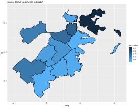
Figure 12: Crime Percentage of Each District

Figure 13: Daily Occurrence of Crime

4.3 Analysis Results

4.3.1 Prediction of Incident Reason

To evaluate the prediction of Incident Reason , we randomly split data into training set and testing set, and follow the measure described in Section 3.2. Table 15 presents the accuracy of naive and hierarchical random forest and Figure 15 shows percentage of crime category 1-3 among the first 3 highest racial groups’ prediction.

	Prediction Accuracy
With proxy	81.40%
Without proxy	81.46%

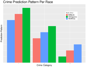
Figure 14: Prediction Accuracy

Figure 15: Prediction Pattern Among Each Racial Group

4.3.2 Prediction of Daily Occurrence

The daily occurrence can be perceived as time series. To this end, we consider a simple AR(1) model. i.e., a specific day’s predication is based on the previous day’s covariates. We also need to modify the categorical covariates to the daily occurrence proportion of the corresponding category. i.e., Larceny happened 5 time out of 50 occurrence on a day, then the occurence proportion of Larceny will be 10%. Additionally, the data split can not be random as the previous settings since it will destroy temporal correlation. To this end, we use the data before 2014 as training set and the data in 2014 as testing set. Figure 17 shows the predicted pattern for 2014 by hierarchical random forest and naive random forest versus true observations with 90% prediction interval and Table 15 shows bias, standard deviation, MSE and percentage of observations falls into the corresponding prediction interval.

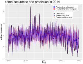
Figure 16: Prediction Pattern for 2014

	without proxy	with proxy
bias	-0.2068	0.4424
SD	27.86094	28.56482
MSE	132.5911	119.1158
Percentage of Observation within PI	73.69%	74.52%

Figure 17: Bias, SD, MSE and Percentage of Observation within PI

5 Concluding Remarks

To recap, covariates like race are prohibited by law because it is potentially related to racial discrimination. To circumvent this problem, we propose a hierarchical random forest model to implicitly use protected classes as latent covariates. We demonstrate the usefulness and comparable results of our model by substantial simulations and real data application. The values of this analysis and prediction are to help scheduling police patrol or targeting suspects. In real application, selecting potential proxy is subjective but should be on the principle of minimizing controversy. Further research could focus on developing some criteria for such proxy.

References

- (1)
- Breiman (2001) Breiman, L. (2001), ‘Random forests’, Machine learning 45(1), 5–32.
- Chen et al. (2019) Chen, J., Kallus, N., Mao, X., Svacha, G. and Udell, M. (2019), Fairness under unawareness: Assessing disparity when protected class is unobserved, in ‘Proceedings of the Conference on Fairness, Accountability, and Transparency’, pp. 339–348.
- Coulston et al. (2016) Coulston, J. W., Blinn, C. E., Thomas, V. A. and Wynne, R. H. (2016), ‘Approximating prediction uncertainty for random forest regression models’, Photogrammetric Engineering & Remote Sensing 82(3), 189–197.
- Jaro (1989) Jaro, M. A. (1989), ‘Advances in record-linkage methodology as applied to matching the 1985 census of tampa, florida’, Journal of the American Statistical Association 84(406), 414–420.
- Larson et al. (2016) Larson, J., Mattu, S., Kirchner, L. and Angwin, J. (2016), ‘How we analyzed the compas recidivism algorithm’, ProPublica (5 2016) 9.
- Lin and Jeon (2006) Lin, Y. and Jeon, Y. (2006), ‘Random forests and adaptive nearest neighbors’, Journal of the American Statistical Association 101(474), 578–590.
- Meinshausen (2006) Meinshausen, N. (2006), ‘Quantile regression forests’, Journal of Machine Learning Research 7(Jun), 983–999.
- Mentch and Hooker (2016) Mentch, L. and Hooker, G. (2016), ‘Quantifying uncertainty in random forests via confidence intervals and hypothesis tests’, The Journal of Machine Learning Research 17(1), 841–881.
- Stekhoven (2015) Stekhoven, D. J. (2015), ‘missforest: Nonparametric missing value imputation using random forest’, Astrophysics Source Code Library .
- Thorndike (1953) Thorndike, R. L. (1953), Who belongs in the family, in ‘Psychometrika’, Citeseer.
- Van der Loo (2014) Van der Loo, M. P. (2014), ‘The stringdist package for approximate string matching’, The R Journal 6(1), 111–122.
- Winkler (1990) Winkler, W. E. (1990), ‘String comparator metrics and enhanced decision rules in the fellegi-sunter model of record linkage.’.
- Zhu et al. (2015) Zhu, R., Zeng, D. and Kosorok, M. R. (2015), ‘Reinforcement learning trees’, Journal of the American Statistical Association 110(512), 1770–1784.