Extraction of autonomous quantum coherences

Artur Slobodeniuk Email: aslobodeniuk@karlov.mff.cuni.cz Affiliation: Department of Optics, Palacký University, 17. listopadu 12, 77146 Olomouc, Czech Republic Affiliation: Department of Condensed Matter Physics, Faculty of Mathematics and Physics, Charles University,
Ke Karlovu 5, CZ-121 16 Prague, Czech Republic
OrcID: 0000-0001-5798-0431
   Tomáš Novotný Email: tno@karlov.mff.cuni.cz Affiliation: Department of Condensed Matter Physics, Faculty of Mathematics and Physics, Charles University,
Ke Karlovu 5, CZ-121 16 Prague, Czech Republic
OrcID: 0000-0001-7014-4155
   Radim Filip Email: filip@optics.upol.cz Affiliation: Department of Optics, Palacký University, 17. listopadu 12, 77146 Olomouc, Czech Republic OrcID: 0000-0003-4114-6068
Abstract

Quantum coherence is an essential resource to gain advantage over classical physics and technology. Recently, it has been proposed that a low-temperature environment can induce quantum coherence of a spin without an external coherent pump. We address a critical question if such coherence is extractable by a weak coupling to an output system dynamically affecting back the spin-environment coupling. Describing the entire mechanism, we prove that such extraction is generically possible for output spins (also oscillators or fields) and, as well, in a fermionic analogue of such a process. We compare the internal spin coherence and output coherence over temperature and characteristic frequencies. The proposed optimal coherence extraction opens paths for the upcoming experimental tests with atomic and solid-state systems.

1 Introduction

Quantum coherence of atomic and solid-state spins is at the core of many quantum technology applications [1] and necessary to gain quantum advantage for modern applications over classical technology. It is highly required for quantum sensing [2, 3], quantum communication [4, 5], quantum simulators [6, 7, 8], energy harvesting [9, 10], quantum thermodynamics [11, 12, 13] and, of course, in quantum computing [14, 15]. It also stimulates a broad recent theoretical analysis [16, 17, 18, 19, 20, 21, 22] and new discussions [23, 24, 25, 26, 27, 28, 29, 30, 31, 32]. The simplest quantum coherence can appear in a single spin as superposition of free-Hamiltonian eigenstates. A classical coherent external force can be used to induce spin quantum coherence. On the other hand, coupling of spin to the surrounding environment typically destroys quantum coherence [33].

Can such a single spin, and later a larger spin ensemble, receive a steady-state quantum coherence without any external coherent drive, purely from a coherent coupling with its environment? If that is possible, quantum technology can be, in principle, more autonomous. Maybe, as broadly discussed, even Nature can already use such coherence to gain quantum advantages without external drive [34, 35]. It might be hard to imagine that a low-temperature environment coherently builds up quantum coherence. However, the recent theoretical considerations predict such an open door. Indeed, single spin coherence can generically appear by cooling the phononic environment to a low temperature [36]. Quantum coherence of the spin rises there from the coherence of engineered interaction with the environment.

Subsequent studies confirmed similar phenomena [37, 38, 39] and also bring the first experimental proposal in the solid-state systems [40]. The path to the first experiments seems to be open. However, an essential aspect remains still unsolved. Is such autonomous coherence extractable, i.e. can an output system continuously and even weakly connected to the spin extract the steady-state coherence? Would such weak extraction not disturb the coherence generation? These essential questions are already critical for a fundamental understanding and detectability of quantum coherence as a resource. Simultaneously, to answer them will be necessary for more autonomous quantum devices and their applications. Apparently, our current picture about an extraction of coherence caused by an external drive is not sufficient. It assumes that strong coherent external drive is largely immune to coupling the output system. As the autonomous coherences appear by an interaction with environment, their extraction is still an open issue.

The existing experimental proposal [40] has opened this key question of extraction of autonomous coherence into an intracavity field. The extraction assumed a weak linear coupling of the cavity field to the spin in a simple static approximation without any back action on the spin and coupling with the environment. For the cavity-field frequency much below the spin frequency and mean spin population almost unchanged (see equation (70) in Supplementary Notes [40]), the spin coherence drives the mean coherent displacement of the high-quality cavity field. It scales only by the spin-cavity coupling strength (see equations (70)-(73) in Supplementary Notes [40]) and is inversely proportional to the field frequency.

Here, we build upon that analysis and propose a minimal extraction mechanism suitable for fields, oscillators, spins, and fermions. We compare that static approximation to our full dynamical description with an essential back action of extraction on spin-environment interaction. In this way, we thoroughly answer the question about autonomous coherence extractability. To provide an in-depth analysis, we adopt the spin as the output system, as illustrated in Fig. 1 (a). However, as the spin is weakly excited, the results remain valid for the oscillator of field mode as the output system. For the sake of completeness, we present an adequate extension to fermionic systems. Importantly, we confirm that the autonomous coherence is generically extractable to all these output systems. It paves a road to the first experimental tests. In the full dynamical description, extracted coherence nontrivially depends on the environment temperature and characteristic system frequencies. For the spin system, we reach coherence maximum asymptotically for a low temperature. Interestingly, the coherence maximum appears at finite temperature for a fermionic analogue. It is stimulating for further proposals to obtain autonomous quantum coherences.

2 Spin-boson model

Figure 1: Extraction of autonomous quantum coherence. (a) Model of the system. The internal spin 11 with a coherence σ1x\langle\sigma_{1}^{x}\rangle interacts with the bosonic degrees of freedom of the environmental bath, represented by the red two-headed arrows. The intensity of interaction with the kk-th bosonic mode is characterized by the weight parameter λk\lambda_{k}. The coupling of the internal spin with the bath is defined by the pair of real parameters f1,f2f_{1},f_{2}. The internal spin interacts with the output spin 22 with a coherence σ2x\langle\sigma_{2}^{x}\rangle via spin-spin coupling term. The strength of coupling is defined by the parameter tt. The bath temperature is TT. (b) Scheme of derivation the coherence of the output spin σ2x\langle\sigma_{2}^{x}\rangle in the static response approximation. The internal spin with the non-zero thermal average σ1z\langle\sigma_{1}^{z}\rangle but vanishing σ1x\langle\sigma_{1}^{x}\rangle (first panel) induces the non-zero shift of the boson degrees of freedom bk+bk\langle b_{k}+b_{k}^{\dagger}\rangle (second panel) via the f1f_{1} term. The bosonic shift acts back on to the output spin via the f2f_{2} term and generates a non-zero coherence of the internal spin σ1x\langle\sigma_{1}^{x}\rangle (third panel). The part of this coherence is transferred to the output spin via the tt term and generates non-zero coherence σ2x\langle\sigma_{2}^{x}\rangle (fourth panel). (c) The sketch of the temperature dependence of the extracted coherence σ2x\langle\sigma_{2}^{x}\rangle derived in the static response approximation (blue curve) and in the quantum full dynamical response (gray curve).

To analyze the extraction of autonomous quantum coherence, we minimally extend the model [36, 40]. Fig. 1 (a) schematically illustrates the model we use to describe the extraction of quantum coherence. The Hamiltonian of the model H=H12+HB+HB1H=H_{12}+H_{B}+H_{B1} consists of three parts, described below. We consider a single (internal) spin 11 coupled weakly with a strength tt to an output spin 22. The output spin 22 will extract the quantum coherence of the initial spin 11. The overall two-spin Hamiltonian

H12=ω12σ1z+ω22σ2z+t(σ1+σ2+σ2+σ1),H_{12}=\frac{\hbar\omega_{1}}{2}\sigma_{1}^{z}+\frac{\hbar\omega_{2}}{2}\sigma_{2}^{z}+\hbar t(\sigma_{1}^{+}\sigma_{2}^{-}+\sigma_{2}^{+}\sigma_{1}^{-}), (1)

describes the spin-spin coupling, where ω1\hbar\omega_{1} and ω2\hbar\omega_{2} are the energies of the first and second spins, respectively. Here the Pauli spin operators σ1j\sigma_{1}^{j} and σ2j\sigma_{2}^{j} (with j=x,y,zj=x,y,z) correspond to the spins 11 and 22. The raising σn+\sigma_{n}^{+} and lowering σn\sigma_{n}^{-} operators of n(=1,2)n(=1,2)-th spin are σn±=(σnx±iσny)/2\sigma_{n}^{\pm}=(\sigma_{n}^{x}\pm i\sigma_{n}^{y})/2. Note that, the coupling term in Eq. (1) is not able to generate the output coherence if it is not present in the internal spin. As the coupling is weak tω1,ω2t\ll\omega_{1},\omega_{2} and the internal spin 11 is weakly excited, any excitation of the output spin 22 will be small too. In this limit, we can equivalently consider the output spin 22 as the two lowest levels of an oscillator or field of radiation. It generalizes the description and covers detailed analysis also for the proposal [40]. Numerical simulations check the validity of weak coupling approximation for small t<ω1,ω2t<\omega_{1},\omega_{2}, see Appendices H and I for details.

As in the previous works [36, 40], the internal spin 11 is coupled to a multimode phononic bath (generally, bosonic bath) described by the Hamiltonian

HB=kΩkbkbk,H_{B}=\sum_{k}\Omega_{k}b_{k}^{\dagger}b_{k}, (2)

through the engineered spin-boson coupling

HB1=(f1σ1z+f2σ1x)kλk(bk+bk).H_{B1}=(f_{1}\sigma_{1}^{z}+f_{2}\sigma_{1}^{x})\sum_{k}\lambda_{k}(b_{k}^{\dagger}+b_{k}). (3)

The boson system is described by creation bkb_{k}^{\dagger} and annihilation bkb_{k} operators and spectrum Ωk>0\Omega_{k}>0. Subscript kk parameterizes all the boson degrees of freedom. The interaction between the internal spin 11 and bosons are defined by real-valued coupling constants f1f_{1} and f2f_{2} [36, 40]. Steady-state equilibrium quantum coherence autonomously appears at a low temperature if both f1,f2f_{1},f_{2} are non-vanishing [36, 40]. In Ref. [36], the Hamiltonian without the output subsystem was considered, and hence the extraction of autonomous quantum coherence remained an open problem. In Ref. [40], a perturbative static analysis of the extraction predicted a coherence of the output cavity-field coupled to the spin 11. As is described in Fig. 1 (b), such a static approximation does not consider the crucial back-action of the output system on the spin-environment. Although, the static approach is an inspiring approximation, the complete dynamical description is needed to address extractability convincingly. In such a dynamical theory, extractable quantum coherence can not only change, as depicted schematically at Fig. 1 (c), but it could also potentially vanish, which would be critical.

In the full treatment of the perturbative analysis, quantum coherence of the output spin 22 in our spin model (see Appendices A, B, C, D, and E for details) can reach

σ2xT=4f1f2tω2tanh(βω22)tanh(βω12)0dξ(ξ)ξcoth(βξ2)ω1coth(βω12)ξ(ξ22ω12),\displaystyle\langle\sigma_{2}^{x}\rangle_{T}=\frac{4f_{1}f_{2}t}{\omega_{2}}\tanh\Big(\frac{\beta\hbar\omega_{2}}{2}\Big)\tanh\Big(\frac{\beta\hbar\omega_{1}}{2}\Big)\int_{0}^{\infty}d\xi\,\mathcal{I}(\xi)\frac{\xi\coth\Big(\frac{\beta\xi}{2}\Big)-\hbar\omega_{1}\coth\Big(\frac{\beta\hbar\omega_{1}}{2})}{\xi(\xi^{2}-\hbar^{2}\omega_{1}^{2})}, (4)

where β(kBT)1\beta\equiv(k_{B}T)^{-1} is the inverse temperature in energy units, kBk_{B} is the Boltzmann constant, TT is the temperature of the system in Kelvin scale and (ξ)kλk2δ(ξΩk)\mathcal{I}(\xi)\equiv\sum_{k}\lambda_{k}^{2}\delta(\xi-\Omega_{k}) is the bath spectral density function. Simultaneously, the mean value σ2yT\langle\sigma_{2}^{y}\rangle_{T} is zero. The extracted quantum coherence is proportional to f1f_{1} and f2f_{2} as in the previous analysis [40]. Similarly, it linearly scales with the coupling strength tt of the interaction term in Eq. (1). The frequency dependence on ω1\omega_{1} and ω2\omega_{2} is factorized. Note that the coherence of the second spin scales linearly with the coherence of the first spin

σ1xT=4f1f2tanh(βω12)0dξ(ξ)ξcoth(βξ2)ω1coth(βω12)ξ(ξ22ω12),\langle\sigma_{1}^{x}\rangle_{T}=-4f_{1}f_{2}\tanh\Big(\frac{\beta\hbar\omega_{1}}{2}\Big)\int_{0}^{\infty}d\xi\,\mathcal{I}(\xi)\frac{\xi\coth\Big(\frac{\beta\xi}{2}\Big)-\hbar\omega_{1}\coth\Big(\frac{\beta\hbar\omega_{1}}{2}\Big)}{\xi\left(\xi^{2}-\hbar^{2}\omega_{1}^{2}\right)}, (5)

derived in Appendix F and satisfies the relation

σ2xT=tω2tanh(βω22)σ1xT,\langle\sigma_{2}^{x}\rangle_{T}=-\frac{t}{\omega_{2}}\tanh\Big(\frac{\beta\hbar\omega_{2}}{2}\Big)\langle\sigma_{1}^{x}\rangle_{T}, (6)

valid for any spectral density function (ξ)\mathcal{I}(\xi). This property can be easily observed in the static approximation (see details in Appendix G), where the coherence of the second spin is derived in three steps, depicted in Fig. 1 (b). In the first step, supposing the smallness of the parameter tt, one considers the spins as non-interacting and estimates the non-zero thermal average of the first spin σ1zTst=tanh(βω1/2)\langle\sigma_{1}^{z}\rangle_{T}^{st}=-\tanh(\beta\hbar\omega_{1}/2) (first panel in Fig. 1 (b)). Here, the superscript “st” means “static”. Then, replacing the operator σ1z\sigma_{1}^{z} by its average value σ1zTst\langle\sigma_{1}^{z}\rangle_{T}^{st}, one gets the linear in (bk+bk)(b_{k}+b_{k}^{\dagger}) correction to the bosonic Hamiltonian. This correction causes the non-zero average value bk+bkTst=2f1σ1zTstλk/Ωk\langle b_{k}+b_{k}^{\dagger}\rangle_{T}^{st}=-2f_{1}\langle\sigma_{1}^{z}\rangle_{T}^{st}\lambda_{k}/\Omega_{k} for the kk-th bosonic mode (second panel in Fig. 1 (b)). In the second step, the average bk+bkTst\langle b_{k}+b_{k}^{\dagger}\rangle_{T}^{st} generates the non-zero coherence of the first spin σ1xTst4f1f2[σ1zTst]2Ω/(ω1)\langle\sigma_{1}^{x}\rangle^{st}_{T}\approx-4f_{1}f_{2}[\langle\sigma_{1}^{z}\rangle_{T}^{st}]^{2}\Omega/(\hbar\omega_{1}) due to the f2σ1xf_{2}\sigma_{1}^{x} term in Hamiltonian (3) (third panel in Fig. 1 (b)). Here Ωkλk2/Ωk=0dξ(ξ)/ξ\Omega\equiv\sum_{k}\lambda_{k}^{2}/\Omega_{k}=\int_{0}^{\infty}d\xi\,\mathcal{I}(\xi)/\xi. Finally, σ1xTst\langle\sigma_{1}^{x}\rangle_{T}^{st} induces the non-zero coherence of the second spin σ2xTst(t/ω2)tanh(βω2/2)σ1xTst\langle\sigma_{2}^{x}\rangle_{T}^{st}\approx-(t/\omega_{2})\tanh(\beta\hbar\omega_{2}/2)\langle\sigma_{1}^{x}\rangle_{T}^{st} due to the spin-spin interaction term in Hamiltonian (1) (fourth panel in Fig. 1 (b)). Note that the obtained result is valid only if t|ω1ω2|,ω1,ω2t\ll|\omega_{1}-\omega_{2}|,\omega_{1},\omega_{2}, since under these conditions both spins can be considered separately and weakly interacting, while the results (4) and (5) are valid also for ω1=ω2\omega_{1}=\omega_{2} case (see details in Appendices H and I).

Both temperature and frequency dependency, however, needs more detailed analysis beyond the static approximation. For the generic case of the ohmic spectral density function (ξ)=Aξexp(ξ/ωc)\mathcal{I}(\xi)=A\xi\exp(-\xi/\hbar\omega_{c}) [41, 42], the coherence expression reads

σ2xT=4Af1f2tω2tanh(βω22)tanh(βω12)(ω1ωc,βω1),\langle\sigma_{2}^{x}\rangle_{T}=\frac{4Af_{1}f_{2}t}{\omega_{2}}\tanh\left(\frac{\beta\hbar\omega_{2}}{2}\right)\tanh\left(\frac{\beta\hbar\omega_{1}}{2}\right)\mathcal{F}\Big(\frac{\omega_{1}}{\omega_{c}},\beta\hbar\omega_{1}\Big), (7)

where

(ω1ωc,βω1)=0dxeω1ωcxxcoth(βω1x2)coth(βω12)x21,\mathcal{F}\Big(\frac{\omega_{1}}{\omega_{c}},\beta\hbar\omega_{1}\Big)=\int_{0}^{\infty}dx\,e^{-\frac{\omega_{1}}{\omega_{c}}x}\,\frac{x\coth\left(\frac{\beta\hbar\omega_{1}x}{2}\right)-\coth\left(\frac{\beta\hbar\omega_{1}}{2}\right)}{x^{2}-1}, (8)

is a dimensionless function of parameters ω1/ωc\omega_{1}/\omega_{c} and βω1\beta\hbar\omega_{1}. In the low-temperature limit βω11\beta\hbar\omega_{1}\gg 1, quantum coherence reaches

σ2xT4Af1f2tω2tanh(βω22)[eω1ωcEi(ω1ωc)π23β22ω12],\langle\sigma_{2}^{x}\rangle_{T}\approx\frac{4Af_{1}f_{2}t}{\omega_{2}}\tanh\left(\frac{\beta\hbar\omega_{2}}{2}\right)\Big[-e^{\frac{\omega_{1}}{\omega_{c}}}\textrm{Ei}\Big(-\frac{\omega_{1}}{\omega_{c}}\Big)-\frac{\pi^{2}}{3\beta^{2}\hbar^{2}\omega_{1}^{2}}\Big], (9)

where Ei(x)=xdzez/z\textrm{Ei}(x)=-\int_{-x}^{\infty}dz\,e^{-z}/z is the exponential integral function [43].

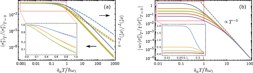
Figure 2: Normalized autonomous coherences in the spin-boson model. (a) Log-log scale plot of normalized coherences σ2xT/σ2xT=0\langle\sigma_{2}^{x}\rangle_{T}/\langle\sigma_{2}^{x}\rangle_{T=0} (solid lines) and σ1xT/σ1xT=0\langle\sigma_{1}^{x}\rangle_{T}/\langle\sigma_{1}^{x}\rangle_{T=0} (dashed lines) for different values of ω1/ωc=0.01,1,100\omega_{1}/\omega_{c}=0.01,1,100 (blue, yellow and green curves, respectively) for the particular case of ω2/ω1=3\omega_{2}/\omega_{1}=3 as a function of temperature TT. Here ωc\omega_{c} is the cut-off energy of the bosonic spectral function of the ohmic type. The inset is the log-linear scale plot of the same functions with the same color notation and parameters. It represents the low-temperature behavior of normalized coherences. The extractable coherence of the spin 22 starts to increase fast for kBT<ω1k_{B}T<\hbar\omega_{1} and saturates sooner at the maximum for smaller ω1/ωc\omega_{1}/\omega_{c}. The backaction of the extraction process does not slow coherence increase in the low-temperature region. (b) Log-log scale plot of absolute value of dimensionless ratio σ2xT/σ1xT=0\langle\sigma_{2}^{x}\rangle_{T}/\langle\sigma_{1}^{x}\rangle_{T=0} multiplied by the normalization factor ω1/t\omega_{1}/t for ω1/ωc=0.01\omega_{1}/\omega_{c}=0.01 and different values of ω2/ω1=0.5,2,4,8,16\omega_{2}/\omega_{1}=0.5,2,4,8,16 (blue, yellow, green, red and purple curves, respectively) as a function of temperature TT. It represents the dependence of the coherence σ2xT\langle\sigma_{2}^{x}\rangle_{T} on ω2\omega_{2}. The gray dashed line depicts the asymptote of all curves, which scales as T3T^{-3}. The inset shows the linear-log plot of the same functions with the same color notation and parameters at small temperatures. It is advantageous to reach ω2/ω1<1\omega_{2}/\omega_{1}<1, to extract quantum coherence to the spin 22 more efficiently.

Both the internal spin 11 and output spin 22 coherences, normalized to their asymptotic values at zero temperature, are compared in Fig. 2 (a). Both the coherences increase monotonously with temperature reduction as in the static approximation. They demonstrate nearly linear behavior at log-log scale for the high temperature region kBT/ω11k_{B}T/\hbar\omega_{1}\gg 1. Therefore, the normalized coherences have a power-law dependence,

σ1xT\displaystyle\langle\sigma_{1}^{x}\rangle_{T\rightarrow\infty} f1f2Ω3ω1(βω1)2=f1f2Aωc3ω1(βω1)2,\displaystyle\approx-f_{1}f_{2}\frac{\Omega}{3\hbar\omega_{1}}(\beta\hbar\omega_{1})^{2}=-f_{1}f_{2}A\frac{\omega_{c}}{3\omega_{1}}(\beta\hbar\omega_{1})^{2}, (10)
σ2xT\displaystyle\langle\sigma_{2}^{x}\rangle_{T\rightarrow\infty} f1f2tω1Ω6ω1(βω1)3=Af1f2tω1ωc6ω1(βω1)3,\displaystyle\approx\frac{f_{1}f_{2}t}{\omega_{1}}\frac{\Omega}{6\hbar\omega_{1}}(\beta\hbar\omega_{1})^{3}=\frac{Af_{1}f_{2}t}{\omega_{1}}\frac{\omega_{c}}{6\omega_{1}}(\beta\hbar\omega_{1})^{3}, (11)

which, however, remain valid only for kBTω1k_{B}T\gg\hbar\omega_{1}. Note that the aforementioned power-law behavior remains valid for the case of an arbitrary spectral density function (ξ)\mathcal{I}(\xi) if the condition 0dξ(ξ)/ξ<+\int_{0}^{\infty}d\xi\,\mathcal{I}(\xi)/\xi<+\infty is satisfied (see Eq. (99) in Appendix E). In particular, it is valid for the generalized Ohmic spectral density function (ξ,s)ξsexp(ξ/ωc)\mathcal{I}(\xi,s)\sim\xi^{s}\exp(-\xi/\hbar\omega_{c}) with s>0s>0 (sub-Ohmic for 0<s<10<s<1 and super-Ohmic for s>1s>1, respectively). Extracted spin 22 coherence increases with a larger slope at the log-log scale. At the high-temperature limit, autonomous coherence is relatively negligible. As the temperature reduces to kBTω1k_{B}T\approx\hbar\omega_{1}, both coherences increase almost up to their maximum values and the normalized output coherence gets closer to the internal one. The latter is evident from the inset of Fig. 2 (a). Note that a wider band of the spectral function with smaller ω1/ωc\omega_{1}/\omega_{c} can already stimulate a faster increase of extractable coherence. Reducing temperature further, the coherence saturates when kBT/ω11k_{B}T/\hbar\omega_{1}\ll 1 much earlier for ω1/ωc1\omega_{1}/\omega_{c}\ll 1. It reaches maximum asymptotically at zero temperature. It is advantageous to have ω1/ωc\omega_{1}/\omega_{c} as small as possible to reach a plateau near the maximum of extractable coherence sooner by lowering the temperature. Indeed, the Eq. (6) proves quantum coherence is extractable, expectably, scaled by the coupling strength tt. The extraction depends both on temperature TT and exclusively on ω2\omega_{2}. Frequency ω1\omega_{1} does not advantageously affect the extraction process in this approximation. For large temperature, the transfer coefficient in (6) turns to σ2xT=t2kBTσ1x\langle\sigma_{2}^{x}\rangle_{T}=-\frac{\hbar t}{2k_{B}T}\langle\sigma_{1}^{x}\rangle. High temperatures thus limit the yielding of the extraction process; on the other hand, for small temperatures, the extraction follows σ2xT=tω2σ1x\langle\sigma_{2}^{x}\rangle_{T}=-\frac{t}{\omega_{2}}\langle\sigma_{1}^{x}\rangle and extraction is not limited by the temperature. Lower ω2\omega_{2} is preferable as it increases the extraction. It approaches the result for the static response qualitatively [40].

To visualize dependence of the output spin 22 coherence as a function of temperature for different values of ω2\omega_{2} we consider the following dimensionless ratio

ω1tσ2xTσ1xT=0=ω1ω2tanh(βω22)tanh(βω12)(ω1ωc,βω1)eω1ωcEi(ω1ωc)σ2xT\frac{\omega_{1}}{t}\frac{\langle\sigma_{2}^{x}\rangle_{T}}{\langle\sigma_{1}^{x}\rangle_{T=0}}=\frac{\omega_{1}}{\omega_{2}}\tanh\left(\frac{\beta\hbar\omega_{2}}{2}\right)\tanh\left(\frac{\beta\hbar\omega_{1}}{2}\right)\frac{\mathcal{F}\Big(\frac{\omega_{1}}{\omega_{c}},\beta\hbar\omega_{1}\Big)}{e^{\frac{\omega_{1}}{\omega_{c}}}\textrm{Ei}\Big(-\frac{\omega_{1}}{\omega_{c}}\Big)}\propto\langle\sigma_{2}^{x}\rangle_{T} (12)

Note that for a fixed ratio ω1/ωc\omega_{1}/\omega_{c} the coherence of the second spin at large temperatures becomes independent of ω2\omega_{2} and demonstrates a universal behavior. In particular, this feature can be observed from the plots of the function

|ω1tσ2xTσ1xT=0|Tωc24ω1(βω1)3eω1ωc|Ei(ω1ωc)|T3,\Big|\frac{\omega_{1}}{t}\frac{\langle\sigma_{2}^{x}\rangle_{T}}{\langle\sigma_{1}^{x}\rangle_{T=0}}\Big|_{T\rightarrow\infty}\approx\frac{\omega_{c}}{24\omega_{1}}\frac{(\beta\hbar\omega_{1})^{3}}{e^{\frac{\omega_{1}}{\omega_{c}}}\Big|\textrm{Ei}\Big(-\frac{\omega_{1}}{\omega_{c}}\Big)\Big|}\propto T^{-3}, (13)

for different ω2\omega_{2}. The transfer of coherence from spin 11 to spin 22 is visualized in Fig. 2 (b) for an optimal choice of small ω1/ωc\omega_{1}/\omega_{c} and different ω2/ω1\omega_{2}/\omega_{1}. For high temperatures, kBT/ω11k_{B}T/\hbar\omega_{1}\gg 1, the increase is linear in the log-log plot with the scaling T3T^{-3} as predicted above. The extraction is inefficient, and the temperature reduction down to kBT/ω11k_{B}T/\hbar\omega_{1}\ll 1 is needed to reach efficient transfer of the quantum coherence. A smaller frequency ω2\omega_{2} of the output spin 22 is very advantageous in this low-temperature regime as longer as the perturbation approach holds. Transfer to the output spin 22 coherence is substantially more efficient when ω2<ω1\omega_{2}<\omega_{1}. Together with the previous condition, the optimal extraction to the output spin (and oscillator or field) needs ω2<ω1<ωc\omega_{2}<\omega_{1}<\omega_{c}.

Note that the coherence of the spin 2 in the low-temperature limit βω11\beta\hbar\omega_{1}\gg 1 can be approximated as

σ2xT04f1f2tω1ω20dξ(ξ)[1ξ1ξ+ω1]=4f1f2tω1ω2Ω4f1f2tω1ω20dξ(ξ)ξ+ω1.\displaystyle\langle\sigma_{2}^{x}\rangle_{T\rightarrow 0}\approx\frac{4f_{1}f_{2}t}{\hbar\omega_{1}\omega_{2}}\int_{0}^{\infty}d\xi\,\mathcal{I}(\xi)\Big[\frac{1}{\xi}-\frac{1}{\xi+\hbar\omega_{1}}\Big]=\frac{4f_{1}f_{2}t}{\hbar\omega_{1}\omega_{2}}\Omega-\frac{4f_{1}f_{2}t}{\hbar\omega_{1}\omega_{2}}\int_{0}^{\infty}d\xi\,\frac{\mathcal{I}(\xi)}{\xi+\hbar\omega_{1}}. (14)

The first term of this expression is nothing but the coherence of spin 2 in the static approximation σ2xTst\langle\sigma_{2}^{x}\rangle_{T}^{st} at zero temperature. In this term the contribution of the bosonic bath is fully factorized and represented only by the parameter Ω\Omega. The factorization reflects the fact that the back-action effects are not taken into account in the static approximation. The result is not sensitive to the shape of the spectral density function (ξ)\mathcal{I}(\xi), since two different spectral density functions with the same Ω\Omega give the same value of the coherence σ2xTst\langle\sigma_{2}^{x}\rangle_{T}^{st}. The second term can be called dynamical since it provides the back-action correction to the static contribution. Note that the frequency parameter ω1\omega_{1} of the spin 1 and energy dependent spectral density function (ξ)\mathcal{I}(\xi) are included in the expression inseparably in contrast to the static result. Therefore, the dynamical term is sensitive to the shape of the spectral density function (ξ)\mathcal{I}(\xi). Finally, the second term represents the deviation of the full coherence σ2xT\langle\sigma_{2}^{x}\rangle_{T} form the static result σ2xTst\langle\sigma_{2}^{x}\rangle_{T}^{st} and hence its value as a function of the temperature answers the question depicted in Fig. 1 (c).

Since (ξ)>0\mathcal{I}(\xi)>0, the static approximation provides only the upper bound of the extracted coherence of spin 2 at low temperatures. Therefore, the correct estimation of such a coherence needs a better understanding of the dynamical term. However, it seems that this term doesn’t have an intuitive explanation in terms of the spin-boson model. Moreover, the perturbation analysis of the dynamical contribution in the spin language is bulky due to the non-commutativity of spin operators and the absence of the Wick theorem for them. This makes the analysis of the static and dynamical terms in higher orders of perturbation theory hard.

Therefore, beyond a general interest, it can be also mathematically valuable to rewrite the spin Hamiltonian, for example, in terms of fermions where the Wick theorem is applicable. It allows the use of the Green function technique and, potentially, makes the final result clearer for understanding. This analysis goes beyond the previous theory for the spins [36, 40], and helps to compare the spin and fermionic systems coupled to the same bosonic baths. Additionally, such an analysis can stimulate a broader class of experimental tests and discussions about a coherence in fermionic systems.

3 Fermion-boson model

In order to implement the aforementioned fermionization program, we apply the Jordan-Wigner transformation (see [44] and references therein) to the Hamiltonians (1) and (3). First, we introduce auxiliary (zeroth) subsystem, which is described by the operators {σ0x,σ0y,σ0z}\{\sigma_{0}^{x},\sigma_{0}^{y},\sigma_{0}^{z}\} and has zero energy. Then we replace the spin operators by the fermionic ones an,n=0,1,2a_{n},n=0,1,2, with the standard anti-commutation rules {an,am}=δnm\{a_{n},a_{m}^{\dagger}\}=\delta_{nm}

σ0\displaystyle\sigma_{0}^{-} a0,σ0+a0,σ0z2a0a01,\displaystyle\rightarrow a_{0},\quad\sigma_{0}^{+}\rightarrow a_{0}^{\dagger},\quad\sigma_{0}^{z}\rightarrow 2a_{0}^{\dagger}a_{0}-1, (15)
σn\displaystyle\sigma_{n}^{-} m=0n1(2amam1)an,σn+m=0n1(2amam1)an,σnz2anan1,\displaystyle\rightarrow\prod_{m=0}^{n-1}(2a_{m}^{\dagger}a_{m}-1)a_{n},\quad\sigma_{n}^{+}\rightarrow\prod_{m=0}^{n-1}(2a_{m}^{\dagger}a_{m}-1)a^{\dagger}_{n},\quad\sigma_{n}^{z}\rightarrow 2a_{n}^{\dagger}a_{n}-1, (16)

and make the additional substitutions

σ1z=\displaystyle\sigma_{1}^{z}= 2a1a112a1a1,σ2z=2a2a212a2a2,\displaystyle 2a_{1}^{\dagger}a_{1}-1\rightarrow 2a_{1}^{\dagger}a_{1},\quad\sigma_{2}^{z}=2a_{2}^{\dagger}a_{2}-1\rightarrow 2a_{2}^{\dagger}a_{2}, (17)
σ1x=\displaystyle\sigma_{1}^{x}= (σ1++σ1)(σ1+σ0+σ0+σ1)=(a1a0+a0a1),\displaystyle(\sigma_{1}^{+}+\sigma_{1}^{-})\rightarrow(\sigma_{1}^{+}\sigma_{0}^{-}+\sigma_{0}^{+}\sigma_{1}^{-})=-(a_{1}^{\dagger}a_{0}+a_{0}^{\dagger}a_{1}), (18)

to remove the constant terms, which do not affect the quantum dynamics significantly. Then the overall fermion-boson Hamiltonian takes the following form

HF=\displaystyle H_{F}= ω1a1a1+ω2a2a2t(a1a2+a2a1)+kΩkbkbk+\displaystyle\hbar\omega_{1}a_{1}^{\dagger}a_{1}+\hbar\omega_{2}a_{2}^{\dagger}a_{2}-\hbar t(a_{1}^{\dagger}a_{2}+a_{2}^{\dagger}a_{1})+\sum_{k}\Omega_{k}b_{k}^{\dagger}b_{k}+ (19)
+[2f1a1a1f2(a1a0+a0a1)]kλk(bk+bk)\displaystyle+[2f_{1}a_{1}^{\dagger}a_{1}-f_{2}(a_{1}^{\dagger}a_{0}+a_{0}^{\dagger}a_{1})]\sum_{k}\lambda_{k}(b_{k}^{\dagger}+b_{k})

from the sum of spin-boson Hamiltonians (1), (2) and (3). Note that the fermionization procedure changes a sign of the spin-spin ttt\rightarrow-t and spin-boson f2f2f_{2}\rightarrow-f_{2} interaction terms. In the following, we will use the subscript FF to indicate that we derived the coherences from the fermionized Hamiltonian HFH_{F}.

Considering same ohmic spectral characteristics of bosonic bath as for the previous two-spin analysis, we can define and derive the fermionic coherence of the first spin using the Eq. (18) (see Appendices J and K for details)

σ1xF,Ta1a0+a1a0F=4f1f2Atanh(βω12)[ωc2ω1+12(ω1ωc,βω1)].\langle\sigma_{1}^{x}\rangle_{F,T}\equiv-\langle a_{1}^{\dagger}a_{0}+a_{1}^{\dagger}a_{0}\rangle_{F}=-4f_{1}f_{2}A\tanh\Big(\frac{\beta\hbar\omega_{1}}{2}\Big)\Big[-\frac{\omega_{c}}{2\omega_{1}}+\frac{1}{2}\mathcal{F}\Big(\frac{\omega_{1}}{\omega_{c}},\beta\hbar\omega_{1}\Big)\Big]. (20)

Here F\langle\dots\rangle_{F} is the thermal average with the Hamiltonian HFH_{F}. The final expression represents the leading contribution to the coherence. We define the fermion coherence of the spin 2 by analogy with the expression for the coherence of the spin 1 and obtain

σ2xF,Ta2a0+a0a2F=4tf1f2AΔωF(ω1ωc,βω1,βω2),\langle\sigma_{2}^{x}\rangle_{F,T}\equiv-\langle a_{2}^{\dagger}a_{0}+a_{0}^{\dagger}a_{2}\rangle_{F}=-\frac{4tf_{1}f_{2}A}{\hbar\Delta\omega}\mathcal{F}_{F}\Big(\frac{\omega_{1}}{\omega_{c}},\beta\hbar\omega_{1},\beta\hbar\omega_{2}\Big), (21)

where Δω=ω2ω1\Delta\omega=\omega_{2}-\omega_{1} and

F(ω1ωc,βω1,βω2)=ωcω2n(ω1)[12n(ω2)]+dxeω1ωc|x|𝒦(x),\displaystyle\mathcal{F}_{F}\Big(\frac{\omega_{1}}{\omega_{c}},\beta\hbar\omega_{1},\beta\hbar\omega_{2}\Big)=\frac{\omega_{c}}{\omega_{2}}n(\hbar\omega_{1})[1-2n(\hbar\omega_{2})]+\int_{-\infty}^{\infty}dxe^{-\frac{\omega_{1}}{\omega_{c}}|x|}\mathcal{K}(x), (22)

with frequency-dependent kernel

𝒦(x)=[N(ω1x)+n(ω1)]{x2(x1)Δωω2n[ω1(1x)]x(x1)(x+Δωω1)Δωω1+n(ω2)ω1xω2(x+Δωω1)}.\displaystyle\mathcal{K}(x)=[N(\hbar\omega_{1}x)+n(\hbar\omega_{1})]\Big\{\frac{x}{2(x-1)}\frac{\Delta\omega}{\omega_{2}}-\frac{n[\hbar\omega_{1}(1-x)]x}{(x-1)(x+\frac{\Delta\omega}{\omega_{1}})}\frac{\Delta\omega}{\omega_{1}}+\frac{n(\hbar\omega_{2})\omega_{1}x}{\omega_{2}(x+\frac{\Delta\omega}{\omega_{1}})}\Big\}. (23)

We introduced the notations for the Bose-Einstein N(ξ)=(eβξ1)1N(\xi)=(e^{\beta\xi}-1)^{-1} and the Fermi-Dirac n(ξ)=(eβξ+1)1n(\xi)=(e^{\beta\xi}+1)^{-1} distributions for brevity. Note that the coherence of each spin is a sum of the Hartree and Fock contributions (see Appendices L, M, N and O for details). It turns out that the Hartree contribution of j(=1,2)j(=1,2)-th spin coincides with the fermionic coherence of the jj-th spin obtained in the static approximation (see Appendix P)

σ1xF,Tst4f1f2Ωω1n(ω1)tanh(βω12),\langle\sigma_{1}^{x}\rangle_{F,T}^{st}\approx\frac{4f_{1}f_{2}\Omega}{\hbar\omega_{1}}n(\hbar\omega_{1})\tanh\Big(\frac{\beta\hbar\omega_{1}}{2}\Big), (24)
σ2xF,Tst4f1f2ΩtΔωn(ω1)[tanh(βω12)ω1tanh(βω22)ω2].\langle\sigma_{2}^{x}\rangle_{F,T}^{st}\approx\frac{4f_{1}f_{2}\Omega t}{\hbar\Delta\omega}n(\hbar\omega_{1})\left[\frac{\tanh\Big(\frac{\beta\hbar\omega_{1}}{2}\Big)}{\omega_{1}}-\frac{\tanh\Big(\frac{\beta\hbar\omega_{2}}{2}\Big)}{\omega_{2}}\right]. (25)

Like in the previous spin-boson case, the influence of the boson bath is fully factorized and represented by the same parameter Ω\Omega for these static terms. The factorization has a natural explanation in the fermion picture. Namely, it comes from the structure of the expression for the Hartree term (see Eq. (164) in Appendix K). Then, the dynamical contribution to the fermion coherences is defined by the Fock terms. Again, similarly to the spin-boson model, the mutual influence of the bosonic bath and the fermion subsystem are not separated in such a case. This property can be seen from the expression for the Fock contribution (see Eq. (163) in Appendix K). The clear physical meaning of the static and dynamical terms in the fermion system provides the potential opportunity to understand better the corresponding terms in spin systems via their fermionization.

The final relation between the internal and output coherence reads

σ2xF,T=tω2σ1xF,T[2ω2Δωcoth(βω12)F(ω1ωc,βω1,βω2)ωcω1(ω1ωc,βω1)]=tω2σ1xF,T(T).\displaystyle\langle\sigma_{2}^{x}\rangle_{F,T}=\frac{t}{\omega_{2}}\langle\sigma_{1}^{x}\rangle_{F,T}\left[-\frac{2\omega_{2}}{\Delta\omega}\coth\Big(\frac{\beta\hbar\omega_{1}}{2}\Big)\frac{\mathcal{F}_{F}\Big(\frac{\omega_{1}}{\omega_{c}},\beta\hbar\omega_{1},\beta\hbar\omega_{2}\Big)}{\frac{\omega_{c}}{\omega_{1}}-\mathcal{F}\Big(\frac{\omega_{1}}{\omega_{c}},\beta\hbar\omega_{1}\Big)}\right]=\frac{t}{\omega_{2}}\langle\sigma_{1}^{x}\rangle_{F,T}\mathcal{R}(T). (26)

Note that the ratio (T)\mathcal{R}(T) is a function of both ω1\omega_{1} and ω2\omega_{2} parameters, while the same ratio for the spin-boson system (see Eq. (6)) is only a function of ω2\omega_{2}. Similarly as for the spin coherence, we normalize (20) and (21) to their values at zero temperature

σ1xF,T=0\displaystyle\langle\sigma_{1}^{x}\rangle_{F,T=0} =2f1f2A[ωcω1+eω1ωcEi(ω1ωc)],σ2xF,T=0=tω2σ1xF,T=0,\displaystyle=2f_{1}f_{2}A\Big[\frac{\omega_{c}}{\omega_{1}}+e^{\frac{\omega_{1}}{\omega_{c}}}\textrm{Ei}\Big(-\frac{\omega_{1}}{\omega_{c}}\Big)\Big],\quad\langle\sigma_{2}^{x}\rangle_{F,T=0}=\frac{t}{\omega_{2}}\langle\sigma_{1}^{x}\rangle_{F,T=0}, (27)

which simplifies their analysis to

σ1xF,Tσ1xF,T=0\displaystyle\frac{\langle\sigma_{1}^{x}\rangle_{F,T}}{\langle\sigma_{1}^{x}\rangle_{F,T=0}} =tanh(βω12)ωcω1(ω1ωc,βω1)ωcω1+eω1ωcEi(ω1ωc),\displaystyle=\tanh\left(\frac{\beta\hbar\omega_{1}}{2}\right)\frac{\frac{\omega_{c}}{\omega_{1}}-\mathcal{F}\Big(\frac{\omega_{1}}{\omega_{c}},\beta\hbar\omega_{1}\Big)}{\frac{\omega_{c}}{\omega_{1}}+e^{\frac{\omega_{1}}{\omega_{c}}}\textrm{Ei}\Big(-\frac{\omega_{1}}{\omega_{c}}\Big)}, (28)
σ2xF,Tσ2xF,T=0\displaystyle\frac{\langle\sigma_{2}^{x}\rangle_{F,T}}{\langle\sigma_{2}^{x}\rangle_{F,T=0}} =2ω2ΔωF(ω1ωc,βω1,βω2)ωcω1+eω1ωcEi(ω1ωc).\displaystyle=-\frac{2\omega_{2}}{\Delta\omega}\frac{\mathcal{F}_{F}\Big(\frac{\omega_{1}}{\omega_{c}},\beta\hbar\omega_{1},\beta\hbar\omega_{2}\Big)}{\frac{\omega_{c}}{\omega_{1}}+e^{\frac{\omega_{1}}{\omega_{c}}}\textrm{Ei}\Big(-\frac{\omega_{1}}{\omega_{c}}\Big)}. (29)

The low-temperature limit relation σ2xF,T=0=tω2σ1xF,T=0\langle\sigma_{2}^{x}\rangle_{F,T=0}=\frac{t}{\omega_{2}}\langle\sigma_{1}^{x}\rangle_{F,T=0} replicates up to the sign the previous result for the spins.

Figure 3: Normalized autonomous coherences in the fermion-boson model. (a) Log-log scale plot of the absolute values of the dimensionless coherences for the fermionic system σ2xF,T/σ2xF,T=0\langle\sigma_{2}^{x}\rangle_{F,T}/\langle\sigma_{2}^{x}\rangle_{F,T=0} (solid lines) and σ1xF,T/σ1xF,T=0\langle\sigma_{1}^{x}\rangle_{F,T}/\langle\sigma_{1}^{x}\rangle_{F,T=0} (dashed lines) for different values of ω1/ωc=0.01,1,100\omega_{1}/\omega_{c}=0.01,1,100 (blue, yellow and green curves, respectively) in the particular case of ω2/ω1=3\omega_{2}/\omega_{1}=3 as a function of temperature TT. The inset shows an advantageous maximum of both internal and output coherences at a finite temperature for ω1>ωc\omega_{1}>\omega_{c}. (b) Log-log scale plot of the absolute value of the dimensionless ratio σ2xF,T/σ1xF,T=0\langle\sigma_{2}^{x}\rangle_{F,T}/\langle\sigma_{1}^{x}\rangle_{F,T=0}, multiplied by the normalization factor ω1/t\omega_{1}/t, for the fixed value of ω1/ωc=0.01\omega_{1}/\omega_{c}=0.01 and different values of ω2/ω1=0.5,2,4,8,16\omega_{2}/\omega_{1}=0.5,2,4,8,16 (blue, yellow, green, red and purple curves, respectively) as a function of temperature TT. It represents the dependence of the coherence σ2xF,T\langle\sigma_{2}^{x}\rangle_{F,T} on ω2\omega_{2}. The gray dashed line depicts the asymptote of all curves, which scales as T2T^{-2}. The inset shows the coherence transfer at the low-temperatures similarly to the spin system.

The normalized internal and output coherences for the fermionic system are visualized in Fig. 3 (a). In the large temperature limit, kBT/ω11k_{B}T/\hbar\omega_{1}\gg 1, the increase of both coherences with decreasing temperature is linear in the log-log plot, similarly as for the spins. It means that also for fermionic systems the increase is only by a power law for large temperatures, and the coherence is negligible. On the other hand, temperature dependence of the internal coherence σ1xF,T/σ1xF,T=0\langle\sigma_{1}^{x}\rangle_{F,T}/\langle\sigma_{1}^{x}\rangle_{F,T=0} is non-monotonous for a large ω1/ωc\omega_{1}/\omega_{c}. It has a maximum near kBT/ω11k_{B}T/\hbar\omega_{1}\approx 1 with a much larger value than at zero temperature. Remarkably, this fermionic model obtains larger internal quantum coherence for a finite temperature away from the zero-temperature limit. Advantageously, the output coherence follows the same non-monotonous tendency for ω1>ωc\omega_{1}>\omega_{c}. The origin of such nontrivial behavior results from interesting competition between Hartree and Fock terms of the inner fermionic coherence. The sudden drop of the output coherence due to zero-crossing is practically irrelevant. The inset shows that the maximum output coherence shifts to the lower temperature with lowering ωc\omega_{c}. However, relative output coherence increase is similar to the internal one. The fermionic system brought new positive phenomena into the autonomous quantum coherence being largest at a finite temperature.

In order to compare the spin and fermion model we consider the high temperature limit

ω1tσ2xF,Tσ1xF,T=0=2ω1ΔωF(ω1ωc,βω1,βω2)ωcω1+eω1ωcEi(ω1ωc)|β0ωc12ω1(βω1)2ωcω1+eω1ωcEi(ω1ωc)(βω1)2,-\frac{\omega_{1}}{t}\frac{\langle\sigma_{2}^{x}\rangle_{F,T\rightarrow\infty}}{\langle\sigma_{1}^{x}\rangle_{F,T=0}}=\frac{2\omega_{1}}{\Delta\omega}\frac{\mathcal{F}_{F}\Big(\frac{\omega_{1}}{\omega_{c}},\beta\hbar\omega_{1},\beta\hbar\omega_{2}\Big)}{\frac{\omega_{c}}{\omega_{1}}+e^{\frac{\omega_{1}}{\omega_{c}}}\textrm{Ei}\Big(-\frac{\omega_{1}}{\omega_{c}}\Big)}\Big|_{\beta\rightarrow 0}\approx\frac{\omega_{c}}{12\omega_{1}}\frac{(\beta\hbar\omega_{1})^{2}}{\frac{\omega_{c}}{\omega_{1}}+e^{\frac{\omega_{1}}{\omega_{c}}}\textrm{Ei}\Big(-\frac{\omega_{1}}{\omega_{c}}\Big)}\propto(\beta\hbar\omega_{1})^{2}, (30)

where we have taken into account

F(ω1ωc,βω1,βω2)|β0Δωωc24ω12(βω1)2.\mathcal{F}_{F}\Big(\frac{\omega_{1}}{\omega_{c}},\beta\hbar\omega_{1},\beta\hbar\omega_{2}\Big)\Big|_{\beta\rightarrow 0}\approx\frac{\Delta\omega\omega_{c}}{24\omega_{1}^{2}}(\beta\hbar\omega_{1})^{2}. (31)

Note that the high temperature behavior of the ratio ω1tσ2xF,Tσ1xF,T=0-\frac{\omega_{1}}{t}\frac{\langle\sigma_{2}^{x}\rangle_{F,T\rightarrow\infty}}{\langle\sigma_{1}^{x}\rangle_{F,T=0}} is independent of ω2\omega_{2} and has another power-low dependence T2\propto T^{-2} in comparison with the same ratio for the spin system, where it behaves as T3\propto T^{-3}. Note that the obtained power-law behavior remains the same for the case of an arbitrary spectral density function (ξ)\mathcal{I}(\xi) which satisfies the condition 0dξ(ξ)/ξ<+\int_{0}^{\infty}d\xi\,\mathcal{I}(\xi)/\xi<+\infty (see Eq. (213) in Appendix N). In particular, it is valid for the case of the generalized Ohmic spectral density function (ξ,s)ξsexp(ξ/ωc)\mathcal{I}(\xi,s)\sim\xi^{s}\exp(-\xi/\hbar\omega_{c}) for s>0s>0 (sub-Ohmic for 0<s<10<s<1 and super-Ohmic for s>1s>1, respectively).

The transfer of coherence from internal to output part in the fermionic system is analogical to the spin system. Only at high temperatures, it scales with T2T^{-2} instead of T3T^{-3} as for the spins. The sudden drops caused by the zero-crossings are practically irrelevant. In the relevant low-temperature regime kBT/ω11k_{B}T/\hbar\omega_{1}\leq 1, the transfer improves for ω2<ω1\omega_{2}<\omega_{1} as in the previous spin analysis. For the fermions, the optimal regime to obtain and extract autonomous quantum coherence efficiently at a finite temperature needs ω1ωc\omega_{1}\gg\omega_{c} and ω2<ω1\omega_{2}<\omega_{1}. It is complementary with the spins, where the large band was optimal. Optimal extraction still profits from the small ω2\omega_{2} until the approximation fails.

4 Summary

We have hereby confirmed the extractibility of autonomous quantum coherence for all basic quantum systems coupled to a generic bosonic environment. The results justified a qualitative prediction from static approximation [40]. They proved that the back action of a weak extraction is fortunately not critical for the coherence generation and extraction in the low-temperature limit. Moreover, we obtained the required frequency and temperature dependences that are not reliably predictable from the static approximation. We optimized the extraction for spins (oscillators and fields) and fermions and found different roles of the environment bandwidth to obtain extractable coherence. Importantly, all those effects are numerically confirmed beyond the asymptotic limit for a finite strength of the extraction (detailed analysis is presented in Appendix). Extractability principally opens a way to experimental verifications of proposals with quantum dots [40] and also to others under development in the superconducting circuits [45], electro-mechanical systems [46], and trapped ions [47].

We can extend the systems used to generate and extract quantum coherence. The fermionic system generating a maximum of coherence at a finite temperature kBTω1k_{B}T\leq\hbar\omega_{1} inspires further extensions. We can investigate three-level and four-level models to optimize the proposed methods. It is a viable investigation area as such systems appear for both atomic and solid-state systems. A possible maximum of quantum coherence at the finite temperature in the region kBT>ω1k_{B}T>\hbar\omega_{1} remains an open problem. However, further engineering of the systems and interaction may overcome such a limit. Another open problem is an accumulation of coherence in an output system from many such parallel interactions. Recently, it has been demonstrated in a collision model that multiple environments can enhance quantum coherence substantially [39]. Further research can be focused on coherence distillation and use a possible extension of the protocols to more spins or fermions giving an even more considerable amount of the extractable quantum coherence. Thermodynamical analysis of autonomous coherence has been already initiated too [37]. These directions for immediate exploration illustrate the novelty of this subject in theory and stimulate current experiments. It is very timely as quantum coherence from a low-temperature environment will directly transform quantum sensors and quantum engines to be more autonomous.

5 Acknowledgments

A.S. and R.F. acknowledge the project 20-16577S of the Czech Science Foundation. R.F. acknowledges also LTAUSA19099 of MEYS CR.

References

  • [1] Alexander Streltsov, Gerardo Adesso, and Martin B. Plenio. Colloquium: Quantum coherence as a resource. Rev. Mod. Phys. 89, 041003 (2017).
  • [2] Simon Schmitt, Tuvia Gefen, Felix M. Stürner, Thomas Unden, Gerhard Wolff, Christoph M’́uller, Jochen Scheuer, Boris Naydenov, Matthew Markham, Sebastien Pezzagna, Jan Meijer, Ilai Schwarz, Martin Plenio, Alex Retzker, Liam P. McGuinness, Fedor Jelezko. Submillihertz magnetic spectroscopy performed with a nanoscale quantum sensor. Science 356, 6340, 832-837 (2017).
  • [3] Hengyun Zhou, Joonhee Choi, Soonwon Choi, Renate Landig, Alexander M. Douglas, Junichi Isoya, Fedor Jelezko, Shinobu Onoda, Hitoshi Sumiya, Paola Cappellaro, Helena S. Knowles, Hongkun Park, and Mikhail D. Lukin. Quantum Metrology with Strongly Interacting Spin Systems. Phys. Rev. X 10, 031003 (2020).
  • [4] Andreas Reiserer, Norbert Kalb, Machiel S. Blok, Koen J. M. van Bemmelen, Tim H. Taminiau, Ronald Hanson, Daniel J. Twitchen, and Matthew Markham. Robust Quantum-Network Memory Using Decoherence-Protected Subspaces of Nuclear Spins. Phys. Rev. X 6, 021040 (2016).
  • [5] David D. Awschalom, Ronald Hanson, Jörg Wrachtrup & Brian B. Zhou. Quantum technologies with optically interfaced solid-state spins. Nature Photonics 12, 516–527 (2018).
  • [6] T. Hensgens, T. Fujita, L. Janssen, Xiao Li, C. J. Van Diepen, C. Reichl, W. Wegscheider, S. Das Sarma & L. M. K. Vandersypen. Quantum simulation of a Fermi–Hubbard model using a semiconductor quantum dot array. Nature 548, 70–73 (2017).
  • [7] Robert Drost, Teemu Ojanen, Ari Harju & Peter Liljeroth. & Liljeroth, P. Topological states in engineered atomic lattices. Nature Physics 13, 668–671 (2017).
  • [8] Marlou R. Slot, Thomas S. Gardenier, Peter H. Jacobse, Guido C. P. van Miert, Sander N. Kempkes, Stephan J. M. Zevenhuizen, Cristiane Morais Smith, Daniel Vanmaekelbergh & Ingmar Swart. Experimental realization and characterization of an electronic Lieb lattice. Nature Physics 13, 672-676 (2017).
  • [9] Gregory D. Scholes, Graham R. Fleming, Lin X. Chen, Alán Aspuru-Guzik, Andreas Buchleitner, David F. Coker, Gregory S. Engel, Rienk van Grondelle, Akihito Ishizaki, David M. Jonas, Jeff S. Lundeen, James K. McCusker, Shaul Mukamel, Jennifer P. Ogilvie, Alexandra Olaya-Castro, Mark A. Ratner, Frank C. Spano, K. Birgitta Whaley & Xiaoyang Zhu. Using coherence to enhance function in chemical and biophysical systems. Nature 543, 647–656 (2017).
  • [10] Elisabet Romero, Vladimir I. Novoderezhkin & Rienk van Grondelle. Quantum design of photosynthesis for bio-inspired solar-energy conversion. Nature 543, 647–656 (2017).
  • [11] James Klatzow, Jonas N. Becker, Patrick M. Ledingham, Christian Weinzetl, Krzysztof T. Kaczmarek, Dylan J. Saunders, Joshua Nunn, Ian A. Walmsley, Raam Uzdin, and Eilon Poem. Experimental demonstration of quantum effects in the operation of microscopic heat engines. Phys. Rev. Lett. 122, 110601 (2019).
  • [12] K. Ono, S. N. Shevchenko, T. Mori, S. Moriyama, and Franco Nori. F. Analog of a Quantum Heat Engine Using a Single-Spin Qubit. Phys. Rev. Lett. 125, 166802 (2020).
  • [13] Camille L. Latune, Ilya Sinayskiy & Francesco Petruccione. Roles of quantum coherences in thermal machines. Eur. Phys. J. Spec. Top. (2021).
  • [14] C. E. Bradley, J. Randall, M. H. Abobeih, R. C. Berrevoets, M. J. Degen, M. A. Bakker, M. Markham, D. J. Twitchen, and T. H. Taminiau. A Ten-Qubit Solid-State Spin Register with Quantum Memory up to One Minute. Phys. Rev. X 9, 031045 (2019).
  • [15] C. J. Stephen, B. L. Green, Y. N. D. Lekhai, L. Weng, P. Hill, S. Johnson, A. C. Frangeskou, P. L. Diggle, Y.-C. Chen, M. J. Strain, E. Gu, M. E. Newton, J. M. Smith, P. S. Salter, and G. W. Morley. Deep Three-Dimensional Solid-State Qubit Arrays with Long-Lived Spin Coherence. Phys. Rev. Applied 12, 064005 (2019).
  • [16] Flavio Del Santo and Borivoje Dakić. Coherence Equality and Communication in a Quantum Superposition. Phys. Rev. Lett. 124, 190501 (2020).
  • [17] Flavio Del Santo and Borivoje Dakić. Two-Way Communication with a Single Quantum Particle. Phys. Rev. Lett. 120, 060503 (2018).
  • [18] Kok Chuan Tan, Tyler Volkoff, Hyukjoon Kwon, and Hyunseok Jeong. Quantifying the Coherence between Coherent States. Phys. Rev. Lett. 119, 190405 (2017).
  • [19] Kaonan Micadei, John P. S. Peterson, Alexandre M. Souza, Roberto S. Sarthour, Ivan S. Oliveira, Gabriel T. Landi, Roberto M. Serra, and Eric Lutz. Experimental Validation of Fully Quantum Fluctuation Theorems Using Dynamic Bayesian Networks Phys.Rev.Lett. 127, 180603 (2021).
  • [20] Jose Joaquin Alonso, Eric Lutz, and Alessandro Romito. Thermodynamics of Weakly Measured Quantum Systems. Phys. Rev. Lett. 116, 080403 (2016).
  • [21] J. F. Haase, A. Smirne, J. Kołodyński, R. Demkowicz-Dobrzański, and S. F. Huelga, Fundamental limits to frequency estimation: a comprehensive microscopic perspective. New J. Phys. 20, 053009 (2018).
  • [22] Jan Czajkowski, Krzysztof Pawłowski and Rafał Demkowicz-Dobrzański. Many-body effects in quantum metrology. New J. Phys. 21 053031 (2019).
  • [23] Leonardo Novo, Masoud Mohseni & Yasser Omar. Disorder-assisted quantum transport in suboptimal decoherence regimes. Scientific Reports 6, 18142 (2016).
  • [24] Kaonan Micadei, Gabriel T. Landi, and Eric Lutz. Quantum Fluctuation Theorems beyond Two-Point Measurements. Phys. Rev. Lett. 124, 090602 (2020).
  • [25] María García Díaz, Giacomo Guarnieri, Mauro Paternostro. Quantum work statistics with initial coherence. Entropy 22(11), 1223 (2020).
  • [26] Rafał Demkowicz-Dobrzański, Jan Czajkowski, and Pavel Sekatski. Adaptive Quantum Metrology under General Markovian Noise. Phys. Rev. X 7, 041009 (2017).
  • [27] Stella Seah, Stefan Nimmrichter, and Valerio Scarani. Maxwell’s Lesser Demon: A Quantum Engine Driven by Pointer Measurements. Phys. Rev. Lett. 124, 100603 (2020).
  • [28] Harry J. D. Miller, Giacomo Guarnieri, Mark T. Mitchison, and John Goold. Quantum fluctuations hinder finite-time information erasure near the Landauer limit. Phys. Rev. Lett. 125, 160602 (2020).
  • [29] G. Francica, F. C. Binder, G. Guarnieri, M. T. Mitchison, J. Goold, and F. Plastina. Quantum Coherence and Ergotropy. Phys. Rev. Lett. 125, 180603 (2020).
  • [30] Stella Seah, Stefan Nimmrichter, Daniel Grimmer, Jader P. Santos, Valerio Scarani, and Gabriel T. Landi. Collisional Quantum Thermometry. Phys. Rev. Lett. 123, 180602 (2019).
  • [31] C. L. Latune, I. Sinayskiy & F. Petruccione. Quantum coherence, many-body correlations, and non-thermal effects for autonomous thermal machines. Scientific Reports 9, 3191 (2019).
  • [32] Devashish Tupkary, Abhishek Dhar, Manas Kulkarni, Archak Purkayastha. Fundamental limitations in Lindblad descriptions of systems weakly coupled to baths. Phys. Rev. A 105, 032208 (2022)
  • [33] Wojciech Hubert Zurek. Decoherence, einselection, and the quantum origins of the classical. Rev. Mod. Phys. 75, 715 (2003).
  • [34] Mohseni, M., Omar, Y., Engel, G. S., Plenio, M. Quantum Effects in Biology (Cambridge Univ Press, Cambridge, MA, 2014).
  • [35] Hong-Guang Duan, Valentyn I. Prokhorenko, Richard J. Cogdell, Khuram Ashraf, Amy L. Stevens, Michael Thorwart, and R. J. Dwayne Miller. Nature does not rely on long-lived electronic quantum coherence for photosynthetic energy transfer. PNAS 114 (32) 8493-8498 (2017).
  • [36] Giacomo Guarnieri, Michal Kolář, and Radim Filip. Steady-State Coherences by Composite System-Bath Interactions. Phys. Rev. Lett. 121, 070401 (2018).
  • [37] Giacomo Guarnieri, Daniele Morrone, Barış Çakmak, Francesco Plastina, Steve Campbelle. Non-equilibrium steady-states of memoryless quantum collision models. Phys. Lett. A 384, 24, 126576 (2020).
  • [38] Mike Reppert, Deborah Reppert, Leonardo A. Pachon, and Paul Brumer. Equilibrium stationary coherence in the multilevel spin-boson model. Phys. Rev. A 102, 012211 (2020).
  • [39] Román-Ancheyta, R., Kolář, M., Guarnieri, G., Filip, R. Enhanced steady-state coherences via repeated system-bath interactions. Phys. Rev. A 104, 062209 (2021).
  • [40] Archak Purkayastha, Giacomo Guarnieri, Mark T. Mitchison, Radim Filip & John Goold. Tunable phonon-induced steady-state coherence in a double-quantum-dot charge qubit. npj Quantum Information 6, 27 (2020).
  • [41] H.-P. Breuer, F.Petruccione. The Theory of Open Quantum Systems (Oxford University Press, 2007)
  • [42] U. Weiss. Quantum Dissipative Systems (World Scientific Publishing, 2012)
  • [43] H. Bateman, A. Erdélyi. Higher Transcendental Functions. Vol.2. Bessel Functions, Parabolic Cylinder Functions, Orthogonal Polynomials (McGraw-Hill, 1953).
  • [44] Elliott Lieb,Theodore Schultz, Daniel Mattis. Two soluble models of an antiferromagnetic chain. Annals of Physics 16, 407 (1961).
  • [45] S. Touzard, A. Kou, N. E. Frattini, V. V. Sivak, S. Puri, A. Grimm, L. Frunzio, S. Shankar, and M. H. Devoret. Gated Conditional Displacement Readout of Superconducting Qubits. Phys. Rev. Lett. 122, 080502 (2019).
  • [46] X. Ma, J. J. Viennot, S. Kotler, J. D. Teufel & K. W. Lehnert. Non-classical energy squeezing of a macroscopic mechanical oscillator. Nature Physics 17, 322-326 (2021).
  • [47] M.-L. Cai, Z.-D. Liu, W.-D. Zhao, Y.-K. Wu, Q.-X. Mei, Y. Jiang, L. He, X. Zhang, Z.-C. Zhou & L.-M. Duan. Observation of a quantum phase transition in the quantum Rabi model with a single trapped ion. Nature Communications 12, 1126 (2021).

Appendix A Spin-boson Hamiltonian

We consider the Hamiltonian of two interacting spins coupled to the boson system

H=ω12σ1z+ω22σ2z+t(σ1+σ2+σ2+σ1)+kΩkbkbk+(f1σ1z+f2σ1x)kλk(bk+bk).H=\frac{\omega_{1}}{2}\sigma_{1}^{z}+\frac{\omega_{2}}{2}\sigma_{2}^{z}+t(\sigma_{1}^{+}\sigma_{2}^{-}+\sigma_{2}^{+}\sigma_{1}^{-})+\sum_{k}\Omega_{k}b_{k}^{\dagger}b_{k}+(f_{1}\sigma_{1}^{z}+f_{2}\sigma_{1}^{x})\sum_{k}\lambda_{k}(b_{k}^{\dagger}+b_{k}). (32)

Here σ1j\sigma_{1}^{j} and σ2j\sigma_{2}^{j} (with j=x,y,zj=x,y,z) are the Pauli matrices corresponding to the 11-st and 22-nd spins with the energies ω1\omega_{1} and ω2\omega_{2} respectively.The real valued parameter t>0t>0 defines the coupling between the spins. Note that in this section and in further we consider ω1\omega_{1}, ω2\omega_{2} and tt in energy units for brevity. In order to restore the original frequency units, used in the main text, one needs to make the following substitutions ω1ω1\omega_{1}\rightarrow\hbar\omega_{1}, ω2ω2\omega_{2}\rightarrow\hbar\omega_{2} and ttt\rightarrow\hbar t. The raising σn+\sigma_{n}^{+} and lowering σn\sigma_{n}^{-} operators of n(=1,2)n(=1,2)-th spin are σn±=(σnx±iσny)/2\sigma_{n}^{\pm}=(\sigma_{n}^{x}\pm i\sigma_{n}^{y})/2. The boson system is described by creation bkb_{k}^{\dagger} and annihilation bkb_{k} operators and spectrum Ωk>0\Omega_{k}>0. Subscript kk parameterizes all the boson degrees of freedom. The interaction between spins and bosons are defined by real valued coupling constants f1f_{1} and f2f_{2}. It is convenient to introduce the following notations for spin Hamiltonian

H12=ω12σ1z+ω22σ2z+t(σ1+σ2+σ2+σ1),H_{12}=\frac{\omega_{1}}{2}\sigma_{1}^{z}+\frac{\omega_{2}}{2}\sigma_{2}^{z}+t(\sigma_{1}^{+}\sigma_{2}^{-}+\sigma_{2}^{+}\sigma_{1}^{-}), (33)

boson Hamiltonian

HB=kΩkbkbk,H_{B}=\sum_{k}\Omega_{k}b_{k}^{\dagger}b_{k}, (34)

and the spin-boson coupling term

HB1=(f1σ1z+f2σ1x)kλk(bk+bk).H_{B1}=(f_{1}\sigma_{1}^{z}+f_{2}\sigma_{1}^{x})\sum_{k}\lambda_{k}(b_{k}^{\dagger}+b_{k}). (35)

As a first step we write the spin Hamiltonian in the basis of triplet and singlet states of two spins

|1,1=\displaystyle|1,1\rangle= |1|2,|1,1=|1|2,|1,0=12(|1|2+|1|2),\displaystyle|\uparrow_{1}\rangle|\uparrow_{2}\rangle,\quad|1,-1\rangle=|\downarrow_{1}\rangle|\downarrow_{2}\rangle,\quad|1,0\rangle=\frac{1}{\sqrt{2}}(|\uparrow_{1}\rangle|\downarrow_{2}\rangle+|\downarrow_{1}\rangle|\uparrow_{2}\rangle), (36)
|0,0=\displaystyle|0,0\rangle= 12(|1|2|1|2),\displaystyle\frac{1}{\sqrt{2}}(|\uparrow_{1}\rangle|\downarrow_{2}\rangle-|\downarrow_{1}\rangle|\uparrow_{2}\rangle),

where |n|\uparrow_{n}\rangle and |n|\downarrow_{n}\rangle are the eigenstates of the σnz\sigma_{n}^{z} operators with eigenvalues ±1\pm 1 respectively. In this basis the Hamiltonian has the following matrix form

H12=12[ω1+ω20000ω1ω200002tω1ω200ω1ω22t].H_{12}=\frac{1}{2}\left[\begin{array}[]{cccc}\omega_{1}+\omega_{2}&0&0&0\\ 0&-\omega_{1}-\omega_{2}&0&0\\ 0&0&2t&\omega_{1}-\omega_{2}\\ 0&0&\omega_{1}-\omega_{2}&-2t\end{array}\right]. (37)

The non-zero difference δω=ω1ω20\delta\omega=\omega_{1}-\omega_{2}\neq 0 mixes the spin states with zero angular momentum. We consider their linear combination in order to diagonalize the Hamiltonian matrix

|+,0=cos(θ/2)|1,0+sin(θ/2)|0,0,|,0=sin(θ/2)|1,0+cos(θ/2)|0,0.|+,0\rangle=\cos(\theta/2)|1,0\rangle+\sin(\theta/2)|0,0\rangle,\quad|-,0\rangle=-\sin(\theta/2)|1,0\rangle+\cos(\theta/2)|0,0\rangle. (38)

The matrix becomes diagonal for the case cosθ=2t/4t2+δω2\cos\theta=2t/\sqrt{4t^{2}+\delta\omega^{2}}, sinθ=δω/4t2+δω2\sin\theta=\delta\omega/\sqrt{4t^{2}+\delta\omega^{2}}. The eigenvalues become E1=(ω1+ω2)/2=ωE_{1}=(\omega_{1}+\omega_{2})/2=\omega, E2=(ω1+ω2)/2=ωE_{2}=-(\omega_{1}+\omega_{2})/2=-\omega, E3=t2+δω2/4=ϵE_{3}=\sqrt{t^{2}+\delta\omega^{2}/4}=\epsilon and E4=t2+δω2/4=ϵE_{4}=-\sqrt{t^{2}+\delta\omega^{2}/4}=-\epsilon for the states |1,1|1,1\rangle, |1,1|1,-1\rangle, |+,0|+,0\rangle and |,0|-,0\rangle respectively. The spin operators σ1x\sigma_{1}^{x} and σ1z\sigma_{1}^{z} have the following form in the basis |1,1,|1,1,|+,0,|,0|1,1\rangle,|1,-1\rangle,|+,0\rangle,|-,0\rangle

σ1x=[00sinϕcosϕ00cosϕsinϕsinϕcosϕ00cosϕsinϕ00],σ1z=[1000010000sinθcosθ00cosθsinθ],\sigma_{1}^{x}=\left[\begin{array}[]{cccc}0&0&\sin\phi&-\cos\phi\\ 0&0&\cos\phi&\sin\phi\\ \sin\phi&\cos\phi&0&0\\ -\cos\phi&\sin\phi&0&0\end{array}\right],\quad\sigma_{1}^{z}=\left[\begin{array}[]{cccc}1&0&0&0\\ 0&-1&0&0\\ 0&0&\sin\theta&\cos\theta\\ 0&0&\cos\theta&-\sin\theta\end{array}\right], (39)

where ϕ=π/4θ/2\phi=\pi/4-\theta/2.

Appendix B Perturbation analysis

We treat the Hamiltonian H0=H12+HBH_{0}=H_{12}+H_{B} exactly and HB1H_{B1} as a perturbation [40]. We present the density matrix operator in the form (β=1/T\beta=1/T, TT is the temperature in energetic units)

eβH=eβ(H12+HB)X(β).e^{-\beta H}=e^{-\beta(H_{12}+H_{B})}X(\beta). (40)

Here the operator X(β)X(\beta) is presented as a T\mathrm{T}-exponent

X(β)=T(0βdτH~B1(τ))10βdτH~B1(τ)+0βdτ0τdτH~B1(τ)H~B1(τ),X(\beta)=\mathrm{T}\Big(-\int_{0}^{\beta}d\tau\widetilde{H}_{B1}(\tau)\Big)\approx 1-\int_{0}^{\beta}d\tau\widetilde{H}_{B1}(\tau)+\int_{0}^{\beta}d\tau\int_{0}^{\tau}d\tau^{\prime}\widetilde{H}_{B1}(\tau)\widetilde{H}_{B1}(\tau^{\prime}), (41)

where

H~B1(τ)=eτ(H12+HB)HB1eτ(H12+HB).\widetilde{H}_{B1}(\tau)=e^{\tau(H_{12}+H_{B})}H_{B1}e^{-\tau(H_{12}+H_{B})}. (42)

Then the perturbation term HB1=SB=[f1σ1z+f2σ1x][kλk(bk+bk)]H_{B1}=SB=[f_{1}\sigma_{1}^{z}+f_{2}\sigma_{1}^{x}][\sum_{k}\lambda_{k}(b_{k}^{\dagger}+b_{k})] takes the form

H~B1(τ)=\displaystyle\widetilde{H}_{B1}(\tau)= S~(τ)B~(τ)=\displaystyle\widetilde{S}(\tau)\widetilde{B}(\tau)= (43)
=\displaystyle= [f1eτH12σ1zeτH12+f2eτH12σ1xeτH12][kλk(eτHBbkeτHB+eτHBbkeτHB)].\displaystyle[f_{1}e^{\tau H_{12}}\sigma_{1}^{z}e^{-\tau H_{12}}+f_{2}e^{\tau H_{12}}\sigma_{1}^{x}e^{-\tau H_{12}}\Big]\Big[\sum_{k}\lambda_{k}(e^{\tau H_{B}}b_{k}^{\dagger}e^{-\tau H_{B}}+e^{\tau H_{B}}b_{k}e^{-\tau H_{B}})\Big].

Taking into account the structure of the H12H_{12} and HBH_{B} Hamiltonians and using the notation Λ1(τ)=eτω\Lambda_{1}(\tau)=e^{\tau\omega}, Λ2(τ)=eτϵ\Lambda_{2}(\tau)=e^{\tau\epsilon} we obtain

eτHBbkeτHB=eτΩkbk,eτHBbkeτHB=eτΩkbk,e^{\tau H_{B}}b_{k}^{\dagger}e^{-\tau H_{B}}=e^{\tau\Omega_{k}}b_{k}^{\dagger},\quad e^{\tau H_{B}}b_{k}e^{-\tau H_{B}}=e^{-\tau\Omega_{k}}b_{k}, (44)
σ1z(τ)=eτH12σ1zeτH12=[1000010000sinθΛ22(τ)cosθ00Λ22(τ)cosθsinθ],\displaystyle\sigma_{1}^{z}(\tau)=e^{\tau H_{12}}\sigma_{1}^{z}e^{-\tau H_{12}}=\left[\begin{array}[]{cccc}1&0&0&0\\ 0&-1&0&0\\ 0&0&\sin\theta&\Lambda_{2}^{2}(\tau)\cos\theta\\ 0&0&\Lambda_{2}^{-2}(\tau)\cos\theta&-\sin\theta\end{array}\right],
σ1x(τ)=eτH12σ1xeτH12=\displaystyle\sigma_{1}^{x}(\tau)=e^{\tau H_{12}}\sigma_{1}^{x}e^{-\tau H_{12}}= (49)
=[00Λ1(τ)Λ21(τ)sinϕΛ1(τ)Λ2(τ)cosϕ00Λ11(τ)Λ21(τ)cosϕΛ11(τ)Λ2(τ)sinϕΛ11(τ)Λ2(τ)sinϕΛ1(τ)Λ2(τ)cosϕ00Λ11(τ)Λ21(τ)cosϕΛ1(τ)Λ21(τ)sinϕ00].\displaystyle=\left[\begin{array}[]{cccc}0&0&\Lambda_{1}(\tau)\Lambda_{2}^{-1}(\tau)\sin\phi&-\Lambda_{1}(\tau)\Lambda_{2}(\tau)\cos\phi\\ 0&0&\Lambda_{1}^{-1}(\tau)\Lambda_{2}^{-1}(\tau)\cos\phi&\Lambda_{1}^{-1}(\tau)\Lambda_{2}(\tau)\sin\phi\\ \Lambda_{1}^{-1}(\tau)\Lambda_{2}(\tau)\sin\phi&\Lambda_{1}(\tau)\Lambda_{2}(\tau)\cos\phi&0&0\\ -\Lambda_{1}^{-1}(\tau)\Lambda_{2}^{-1}(\tau)\cos\phi&\Lambda_{1}(\tau)\Lambda_{2}^{-1}(\tau)\sin\phi&0&0\end{array}\right].

For calculation of the averages of any operator we use the symmetrization of the density operator

eβH=12[eβ(H12+HB)X(β)+X(β)eβ(H12+HB)].e^{-\beta H}=\frac{1}{2}\Big[e^{-\beta(H_{12}+H_{B})}X(\beta)+X^{\dagger}(\beta)e^{-\beta(H_{12}+H_{B})}\Big]. (54)

Then the partition function ZZ can be expressed as

Z=Tr[eβH]=Z02X(β)+X(β)0.Z=\mathrm{Tr}[e^{-\beta H}]=\frac{Z_{0}}{2}\langle X(\beta)+X^{\dagger}(\beta)\rangle_{0}. (55)

Here 0=Z01Tr[eβ(H12+HB)]\langle\star\rangle_{0}=Z_{0}^{-1}\mathrm{Tr}[e^{-\beta(H_{12}+H_{B})}\star] is the averaging by the non-interaction density function. The partition function up to second order correction takes the following form

Z=Z0{1+120βdτ0τdτ[H~B1(τ)H~B1(τ)0+H~B1(τ)H~B1(τ)0]}.Z=Z_{0}\Big\{1+\frac{1}{2}\int_{0}^{\beta}d\tau\int_{0}^{\tau}d\tau^{\prime}[\langle\widetilde{H}_{B1}(\tau)\widetilde{H}_{B1}(\tau^{\prime})\rangle_{0}+\langle\widetilde{H}_{B1}^{\dagger}(\tau^{\prime})\widetilde{H}_{B1}^{\dagger}(\tau)\rangle_{0}]\Big\}. (56)

Taking the average over the boson degrees of freedom we get

Z=Z0{1+0βdτ0τdτϕ(ττ)ReS~(τ)S~(τ)0},Z=Z_{0}\Big\{1+\int_{0}^{\beta}d\tau\int_{0}^{\tau}d\tau^{\prime}\phi(\tau-\tau^{\prime})\mathrm{Re}\langle\widetilde{S}(\tau)\widetilde{S}(\tau^{\prime})\rangle_{0}\Big\}, (57)

where we introduced the bosonic correlation function

ϕ(ττ)=B~(τ)B~(τ)0=B~(τ)B~(τ)0=kλk2[eΩk(ττ)bkbk0+eΩk(ττ)bkbk0].\phi(\tau-\tau^{\prime})=\langle\widetilde{B}(\tau)\widetilde{B}(\tau^{\prime})\rangle_{0}=\langle\widetilde{B}^{\dagger}(\tau^{\prime})\widetilde{B}^{\dagger}(\tau)\rangle_{0}=\sum_{k}\lambda_{k}^{2}[e^{\Omega_{k}(\tau-\tau^{\prime})}\langle b_{k}^{\dagger}b_{k}\rangle_{0}+e^{-\Omega_{k}(\tau-\tau^{\prime})}\langle b_{k}b_{k}^{\dagger}\rangle_{0}]. (58)

The spin dependent part takes the form

S~(τ)S~(τ)=f12σ1z(τ)σ1z(τ)+f22σ1x(τ)σ1x(τ)+f1f2σ1z(τ)σ1x(τ)+f1f2σ1x(τ)σ1z(τ).\widetilde{S}(\tau)\widetilde{S}(\tau^{\prime})=f_{1}^{2}\sigma_{1}^{z}(\tau)\sigma_{1}^{z}(\tau^{\prime})+f_{2}^{2}\sigma_{1}^{x}(\tau)\sigma_{1}^{x}(\tau^{\prime})+f_{1}f_{2}\sigma_{1}^{z}(\tau)\sigma_{1}^{x}(\tau^{\prime})+f_{1}f_{2}\sigma_{1}^{x}(\tau)\sigma_{1}^{z}(\tau^{\prime}). (59)

We are interested in the spin sector only, therefore we integrate out the boson degrees of freedom in total density operator and keep only the spin dependent part ϱS=TrB[eβH]/Z\varrho_{S}=\mathrm{Tr}_{B}[e^{-\beta H}]/Z

ϱS=\displaystyle\varrho_{S}= eβH12ZS[10βdτ0τdτϕ(ττ)ReS~(τ)S~(τ)0]+\displaystyle\frac{e^{-\beta H_{12}}}{Z_{S}}\Big[1-\int_{0}^{\beta}d\tau\int_{0}^{\tau}d\tau^{\prime}\phi(\tau-\tau^{\prime})\mathrm{Re}\langle\widetilde{S}(\tau)\widetilde{S}(\tau^{\prime})\rangle_{0}\Big]+
+\displaystyle+ 120βdτ0τdτϕ(ττ)[eβH12ZSS~(τ)S~(τ)+h.c.].\displaystyle\frac{1}{2}\int_{0}^{\beta}d\tau\int_{0}^{\tau}d\tau^{\prime}\phi(\tau-\tau^{\prime})\Big[\frac{e^{-\beta H_{12}}}{Z_{S}}\widetilde{S}(\tau)\widetilde{S}(\tau^{\prime})+\textrm{h.c.}\Big]. (60)

Here we introduced ZS=Tr[eβH12]=2cosh(βω)+2cosh(βϵ)Z_{S}=\mathrm{Tr}[e^{-\beta H_{12}}]=2\cosh(\beta\omega)+2\cosh(\beta\epsilon).

Appendix C Averaging procedure for the second spin operators

We are interested in the averages σ2j=Tr[ϱSσ2j]\langle\sigma_{2}^{j}\rangle=\mathrm{Tr}[\varrho_{S}\sigma_{2}^{j}], where j=x,y,zj=x,y,z. The matrices of corresponding spin operators in the basis {|1,1,|1,1,|+,0,|,0}\{|1,1\rangle,|1,-1\rangle,|+,0\rangle,|-,0\rangle\} are

σ2z=\displaystyle\sigma_{2}^{z}= [1000010000sinθcosθ00cosθsinθ],σ2x=[00cosϕsinϕ00sinϕcosϕcosϕsinϕ00sinϕcosϕ00],\displaystyle\left[\begin{array}[]{cccc}1&0&0&0\\ 0&-1&0&0\\ 0&0&-\sin\theta&-\cos\theta\\ 0&0&-\cos\theta&\sin\theta\end{array}\right],\quad\sigma_{2}^{x}=\left[\begin{array}[]{cccc}0&0&\cos\phi&\sin\phi\\ 0&0&\sin\phi&-\cos\phi\\ \cos\phi&\sin\phi&0&0\\ \sin\phi&-\cos\phi&0&0\end{array}\right],
σ2y=\displaystyle\sigma_{2}^{y}= [00icosϕisinϕ00isinϕicosϕicosϕisinϕ00isinϕicosϕ00].\displaystyle\left[\begin{array}[]{cccc}0&0&-i\cos\phi&-i\sin\phi\\ 0&0&i\sin\phi&-i\cos\phi\\ i\cos\phi&-i\sin\phi&0&0\\ i\sin\phi&i\cos\phi&0&0\end{array}\right].

where ϕ=π/4θ/2\phi=\pi/4-\theta/2. In this basis the procedure of taking trace becomes matrix trace procedure. First we calculate the leading terms

ZSσ2z0=Tr[eβH12σ2z]=2sinθsinh(βϵ)2sinh[βω],ZSσ2x(y)0=Tr[eβH12σ2x(y)]=0.Z_{S}\langle\sigma_{2}^{z}\rangle_{0}=\mathrm{Tr}[e^{-\beta H_{12}}\sigma_{2}^{z}]=2\sin\theta\sinh(\beta\epsilon)-2\sinh[\beta\omega],\,Z_{S}\langle\sigma_{2}^{x(y)}\rangle_{0}=\mathrm{Tr}[e^{-\beta H_{12}}\sigma_{2}^{x(y)}]=0. (73)

Then we introduce the traces of the product of the spin operators

F(τ,τ)\displaystyle F(\tau,\tau^{\prime}) =ZSReS~(τ)S~(τ)0=\displaystyle=Z_{S}\mathrm{Re}\langle\widetilde{S}(\tau)\widetilde{S}(\tau^{\prime})\rangle_{0}=
2f12[cosh(βω)+sin2θcosh(βϵ)+cos2θcosh((β2τ+2τ)ϵ)]+\displaystyle 2f_{1}^{2}\Big[\cosh(\beta\omega)+\sin^{2}\theta\cosh(\beta\epsilon)+\cos^{2}\theta\cosh((\beta-2\tau+2\tau^{\prime})\epsilon)\Big]+
2f22[cos2ϕ{cosh(βϵ(ϵ+ω)(ττ))+cosh(βω(ϵ+ω)(ττ))}]+\displaystyle 2f_{2}^{2}\Big[\cos^{2}\phi\{\cosh(\beta\epsilon-(\epsilon+\omega)(\tau-\tau^{\prime}))+\cosh(\beta\omega-(\epsilon+\omega)(\tau-\tau^{\prime}))\}\Big]+
2f22[sin2ϕ{cosh(βϵ(ϵω)(ττ))+cosh(βω+(ϵω)(ττ))}],\displaystyle 2f_{2}^{2}\Big[\sin^{2}\phi\{\cosh(\beta\epsilon-(\epsilon-\omega)(\tau-\tau^{\prime}))+\cosh(\beta\omega+(\epsilon-\omega)(\tau-\tau^{\prime}))\}\Big], (74)
F1(τ,τ)=Tr\displaystyle F_{1}(\tau,\tau^{\prime})=\mathrm{Tr} [eβH12S~(τ)S~(τ)σ2z+S~(τ)S~(τ)eβH12σ2z]=\displaystyle[e^{-\beta H_{12}}\widetilde{S}(\tau)\widetilde{S}(\tau^{\prime})\sigma_{2}^{z}+\widetilde{S}^{\dagger}(\tau^{\prime})\widetilde{S}^{\dagger}(\tau)e^{-\beta H_{12}}\sigma_{2}^{z}]=
4f12\displaystyle 4f_{1}^{2} [sin3θsinh(βϵ)sinh(βω)+sinθcos2θ{sinh(ϵ(β+2τ2τ))+\displaystyle\Big[\sin^{3}\theta\sinh(\beta\epsilon)-\sinh(\beta\omega)+\sin\theta\cos^{2}\theta\{\sinh(\epsilon(\beta+2\tau^{\prime}-2\tau))+
+sinh(ϵ(β2τ))sinh(ϵ(β2τ))}]+\displaystyle+\sinh(\epsilon(\beta-2\tau^{\prime}))-\sinh(\epsilon(\beta-2\tau))\}\Big]+
4f22\displaystyle 4f_{2}^{2} [sinθsin2ϕsinh(βϵ+(ττ)(ϵω))+\displaystyle\Big[\sin\theta\sin^{2}\phi\sinh(\beta\epsilon+(\tau^{\prime}-\tau)(\epsilon-\omega))+
sinθcos2ϕsinh(βϵ+(ττ)(ω+ϵ))+\displaystyle\sin\theta\cos^{2}\phi\sinh(\beta\epsilon+(\tau^{\prime}-\tau)(\omega+\epsilon))+
cosθsinϕcosϕ{sinh(βϵ+τ(ωϵ)τ(ω+ϵ))\displaystyle\cos\theta\sin\phi\cos\phi\{\sinh(\beta\epsilon+\tau^{\prime}(\omega-\epsilon)-\tau(\omega+\epsilon))-
sinh(βϵτ(ω+ϵ)+τ(ωϵ))}\displaystyle\sinh(\beta\epsilon-\tau^{\prime}(\omega+\epsilon)+\tau(\omega-\epsilon))\}-
sin2ϕsinh(ωβ+(ττ)(ωϵ))cos2ϕsinh(βω+(ττ)(ω+ϵ))],\displaystyle\sin^{2}\phi\sinh(\omega\beta+(\tau^{\prime}-\tau)(\omega-\epsilon))-\cos^{2}\phi\sinh(\beta\omega+(\tau^{\prime}-\tau)(\omega+\epsilon))\Big], (75)
F2(τ,τ)\displaystyle F_{2}(\tau,\tau^{\prime}) =Tr[eβH12S~(τ)S~(τ)σ2x+S~(τ)S~(τ)eβH12σ2x]=\displaystyle=\mathrm{Tr}[e^{-\beta H_{12}}\widetilde{S}(\tau)\widetilde{S}(\tau^{\prime})\sigma_{2}^{x}+\widetilde{S}^{\dagger}(\tau^{\prime})\widetilde{S}^{\dagger}(\tau)e^{-\beta H_{12}}\sigma_{2}^{x}]=
4f1f2[cosθcos2ϕ{cosh(βω+2ϵττ(ω+ϵ))+cosh(ϵ(β2τ)+τ(ω+ϵ))}+\displaystyle 4f_{1}f_{2}\Big[-\cos\theta\cos^{2}\phi\{\cosh(\beta\omega+2\epsilon\tau^{\prime}-\tau(\omega+\epsilon))+\cosh(\epsilon(\beta-2\tau)+\tau^{\prime}(\omega+\epsilon))\}+
+cosθsin2ϕ{cosh(βω2ϵττ(ωϵ))+cosh(ϵ(β2τ)+τ(ϵω))}+\displaystyle+\cos\theta\sin^{2}\phi\{\cosh(\beta\omega-2\epsilon\tau^{\prime}-\tau(\omega-\epsilon))+\cosh(\epsilon(\beta-2\tau)+\tau^{\prime}(\epsilon-\omega))\}+
+sin(2ϕ)sinθ{(cosh(ωτ)cosh(ϵ(βτ))+cosh(τϵ)cosh(ω(βτ))}+\displaystyle+\sin(2\phi)\sin\theta\{(\cosh(\omega\tau^{\prime})\cosh(\epsilon(\beta-\tau^{\prime}))+\cosh(\tau\epsilon)\cosh(\omega(\beta-\tau))\}+
+sin(2ϕ){sinh(ϵτ)sinh(ω(βτ))+sinh(τω)sinh(ϵ(βτ)))}],\displaystyle+\sin(2\phi)\{\sinh(\epsilon\tau^{\prime})\sinh(\omega(\beta-\tau^{\prime}))+\sinh(\tau\omega)\sinh(\epsilon(\beta-\tau)))\}\Big], (76)
Tr[eβH12S~(τ)S~(τ)σ2y+S~(τ)S~(τ)eβH12σ2y]=0.\mathrm{Tr}[e^{-\beta H_{12}}\widetilde{S}(\tau)\widetilde{S}(\tau^{\prime})\sigma_{2}^{y}+\widetilde{S}^{\dagger}(\tau^{\prime})\widetilde{S}^{\dagger}(\tau)e^{-\beta H_{12}}\sigma_{2}^{y}]=0. (77)

Appendix D Integral representation for the spin average values

The average values σ2x\langle\sigma_{2}^{x}\rangle and σ2z\langle\sigma_{2}^{z}\rangle are defined by the convolution integrals of F(τ,τ)F(\tau,\tau^{\prime}), F1(τ,τ)F_{1}(\tau,\tau^{\prime}) and F2(τ,τ)F_{2}(\tau,\tau^{\prime}) with ϕ(ττ)\phi(\tau-\tau^{\prime}) in τ,τ\tau,\tau^{\prime} domain. Such the integration can be done in the following way. We introduce the boson spectral function

(ξ)=kλk2δ(ξΩk)\mathcal{I}(\xi)=\sum_{k}\lambda_{k}^{2}\delta(\xi-\Omega_{k}) (78)

and present ϕ(ττ)\phi(\tau-\tau^{\prime}) in the form

ϕ(ττ)=0dξ(ξ){eξ(ττ)eβξ1+eξ(ττ)eβξeβξ1},\phi(\tau-\tau^{\prime})=\int_{0}^{\infty}d\xi\,\mathcal{I}(\xi)\left\{\frac{e^{\xi(\tau-\tau^{\prime})}}{e^{\beta\xi}-1}+\frac{e^{-\xi(\tau-\tau^{\prime})}e^{\beta\xi}}{e^{\beta\xi}-1}\right\}, (79)

taking into account that Ωk>0\Omega_{k}>0. In this notation we can express the non-zero corrections of average values of spin operators in the form

Δσ2z=σ2zσ2z0=12ZS0βdτ0τdτϕ(ττ)[F1(τ,τ)2σ2z0F(τ,τ)],\Delta\langle\sigma_{2}^{z}\rangle=\langle\sigma_{2}^{z}\rangle-\langle\sigma_{2}^{z}\rangle_{0}=\frac{1}{2Z_{S}}\int_{0}^{\beta}d\tau\int_{0}^{\tau}d\tau^{\prime}\phi(\tau-\tau^{\prime})\Big[F_{1}(\tau,\tau^{\prime})-2\langle\sigma_{2}^{z}\rangle_{0}F(\tau,\tau^{\prime})\Big], (80)
σ2x=σ2xσ2x0=12ZS0βdτ0τdτϕ(ττ)F2(τ,τ),\langle\sigma_{2}^{x}\rangle=\langle\sigma_{2}^{x}\rangle-\langle\sigma_{2}^{x}\rangle_{0}=\frac{1}{2Z_{S}}\int_{0}^{\beta}d\tau\int_{0}^{\tau}d\tau^{\prime}\phi(\tau-\tau^{\prime})F_{2}(\tau,\tau^{\prime}), (81)

since σ2x0=0\langle\sigma_{2}^{x}\rangle_{0}=0. Taking into account the structure of ϕ(ττ)\phi(\tau-\tau^{\prime}) function and introducing the transformation

(ξ)=1eβξ10βdτ0τdτeξ(ττ)(τ,τ),\mathcal{F}(\xi)=\frac{1}{e^{\beta\xi}-1}\int_{0}^{\beta}d\tau\int_{0}^{\tau}d\tau^{\prime}e^{\xi(\tau-\tau^{\prime})}\mathcal{F}(\tau,\tau^{\prime}), (82)

we can write

Δσ2z=σ2zσ2z0=12ZS0dξ(ξ){F1(ξ)F1(ξ)2σ2z0[F(ξ)F(ξ)]},\Delta\langle\sigma_{2}^{z}\rangle=\langle\sigma_{2}^{z}\rangle-\langle\sigma_{2}^{z}\rangle_{0}=\frac{1}{2Z_{S}}\int_{0}^{\infty}d\xi\,\mathcal{I}(\xi)\Big\{F_{1}(\xi)-F_{1}(-\xi)-2\langle\sigma_{2}^{z}\rangle_{0}[F(\xi)-F(-\xi)]\Big\}, (83)
σ2x=12ZS0dξ(ξ){F2(ξ)F2(ξ)}.\langle\sigma_{2}^{x}\rangle=\frac{1}{2Z_{S}}\int_{0}^{\infty}d\xi\,\mathcal{I}(\xi)\Big\{F_{2}(\xi)-F_{2}(-\xi)\Big\}. (84)

Appendix E Detuned spins: the second spin coherence

Let us consider the case when |ω1ω2|t|\omega_{1}-\omega_{2}|\gg t. It corresponds to the situation when the energy levels of considered spins are weakly modified by interaction terms. For this case the calculation of the the averages of spin operators can be simplified. Indeed, we consider the leading terms of cos(θ)\cos(\theta) and sin(θ)\sin(\theta) by small parametr t/|ω1ω2|t/|\omega_{1}-\omega_{2}|

sinθ=\displaystyle\sin\theta= (ω1ω2)4t2+(ω1ω2)2sgn(ω1ω2)[12t2(ω1ω2)2],\displaystyle\frac{(\omega_{1}-\omega_{2})}{\sqrt{4t^{2}+(\omega_{1}-\omega_{2})^{2}}}\approx\text{sgn}(\omega_{1}-\omega_{2})\Big[1-\frac{2t^{2}}{(\omega_{1}-\omega_{2})^{2}}\Big],
cosθ=\displaystyle\cos\theta= 2t4t2+(ω1ω2)22t|ω1ω2|,\displaystyle\frac{2t}{\sqrt{4t^{2}+(\omega_{1}-\omega_{2})^{2}}}\approx\frac{2t}{|\omega_{1}-\omega_{2}|}, (85)

substitute them in the expressions for F(τ,τ)F(\tau,\tau^{\prime}), F1(τ,τ)F_{1}(\tau,\tau^{\prime}) and F2(τ,τ)F_{2}(\tau,\tau^{\prime}) and calculate the corresponding integrals over τ,τ\tau,\tau^{\prime} and ξ\xi. We introduce the notations η=sgn(ω1ω2)\eta=\text{sgn}(\omega_{1}-\omega_{2}) and δ=|ω1ω2|\delta=|\omega_{1}-\omega_{2}| in further calculations for brevity. We focus on the evaluation of the coherence of the second spin operator σ2x\langle\sigma_{2}^{x}\rangle. In order to do it we substitute

sin2θ\displaystyle\sin^{2}\theta\approx 14t2δ2,cos2θ4t2δ2,\displaystyle 1-\frac{4t^{2}}{\delta^{2}},\quad\cos^{2}\theta\approx\frac{4t^{2}}{\delta^{2}},
cos2ϕ=\displaystyle\cos^{2}\phi= 1+sinθ21+η2ηt2δ2,sin2ϕ=1sinθ21η2+ηt2δ2,\displaystyle\frac{1+\sin\theta}{2}\approx\frac{1+\eta}{2}-\frac{\eta t^{2}}{\delta^{2}},\quad\sin^{2}\phi=\frac{1-\sin\theta}{2}\approx\frac{1-\eta}{2}+\frac{\eta t^{2}}{\delta^{2}}, (86)

in Eq. (C) and keep the leading term in the series expansion of this expression by the small parameter t/δt/\delta. We have

F2(τ,τ)=8f1f2tω1ω2\displaystyle F_{2}(\tau,\tau^{\prime})=\frac{8f_{1}f_{2}t}{\omega_{1}-\omega_{2}} [sinh(12(ω1ω2)τ)sinh(12(ω1+ω2)(βτ))+\displaystyle\Big[\sinh\left(\frac{1}{2}\left(\omega_{1}-\omega_{2}\right)\tau^{\prime}\right)\sinh\left(\frac{1}{2}\left(\omega_{1}+\omega_{2}\right)\left(\beta-\tau^{\prime}\right)\right)+
+cosh(12(ω1+ω2)τ)cosh(12(ω1ω2)(βτ))\displaystyle+\cosh\left(\frac{1}{2}\left(\omega_{1}+\omega_{2}\right)\tau^{\prime}\right)\cosh\left(\frac{1}{2}\left(\omega_{1}-\omega_{2}\right)\left(\beta-\tau^{\prime}\right)\right)-
cosh(12(ω1ω2)(β2τ)+ω1τ)\displaystyle-\cosh\left(\frac{1}{2}\left(\omega_{1}-\omega_{2}\right)(\beta-2\tau)+\omega_{1}\tau^{\prime}\right)-
cosh(12β(ω1+ω2)+(ω2ω1)τ+τω1)+\displaystyle-\cosh\left(-\frac{1}{2}\beta\left(\omega_{1}+\omega_{2}\right)+\left(\omega_{2}-\omega_{1}\right)\tau^{\prime}+\tau\omega_{1}\right)+
+sinh(12τ(ω1+ω2))sinh(12(ω1ω2)(βτ))+\displaystyle+\sinh\left(\frac{1}{2}\tau\left(\omega_{1}+\omega_{2}\right)\right)\sinh\left(\frac{1}{2}\left(\omega_{1}-\omega_{2}\right)(\beta-\tau)\right)+
+cosh(12τ(ω1ω2))cosh(12(ω1+ω2)(βτ))].\displaystyle+\cosh\left(\frac{1}{2}\tau\left(\omega_{1}-\omega_{2}\right)\right)\cosh\left(\frac{1}{2}\left(\omega_{1}+\omega_{2}\right)(\beta-\tau)\right)\Big]. (87)

After integration over τ,τ\tau,\tau^{\prime} we get

F2(ξ)F2(ξ)=32f1f2tsinh(βω22)sinh(βω12)(ξcoth(βξ2)ω1coth(βω12))ξω2(ξ2ω12)F_{2}(\xi)-F_{2}(-\xi)=\frac{32f_{1}f_{2}t\sinh\left(\frac{\beta\omega_{2}}{2}\right)\sinh\left(\frac{\beta\omega_{1}}{2}\right)\left(\xi\coth\left(\frac{\beta\xi}{2}\right)-\omega_{1}\coth\left(\frac{\beta\omega_{1}}{2}\right)\right)}{\xi\omega_{2}\left(\xi^{2}-\omega_{1}^{2}\right)} (88)

Therefore the coherence σ2x\langle\sigma_{2}^{x}\rangle takes the form

σ2x=\displaystyle\langle\sigma_{2}^{x}\rangle= 12ZS0dξ(ξ){F2(ξ)F2(ξ)}=\displaystyle\frac{1}{2Z_{S}}\int_{0}^{\infty}d\xi\,\mathcal{I}(\xi)\Big\{F_{2}(\xi)-F_{2}(-\xi)\Big\}=
=\displaystyle= 4f1f2tω2tanh(βω22)tanh(βω12)0dξ(ξ)ξcoth(βξ2)ω1coth(βω12)ξ(ξ2ω12),\displaystyle\frac{4f_{1}f_{2}t}{\omega_{2}}\tanh\Big(\frac{\beta\omega_{2}}{2}\Big)\tanh\Big(\frac{\beta\omega_{1}}{2}\Big)\int_{0}^{\infty}d\xi\,\mathcal{I}(\xi)\frac{\xi\coth\Big(\frac{\beta\xi}{2}\Big)-\omega_{1}\coth\Big(\frac{\beta\omega_{1}}{2}\Big)}{\xi(\xi^{2}-\omega_{1}^{2})}, (89)

where we use ZSZ_{S} in the leading order by t/δt/\delta: ZS=4cosh(βω1/2)cosh(βω2/2)Z_{S}=4\cosh(\beta\omega_{1}/2)\cosh(\beta\omega_{2}/2).

For the particular case of spectral density function (ξ)=Aξexp(ξ/ωc)\mathcal{I}(\xi)=A\xi\exp(-\xi/\omega_{c}) this expression reads

σ2x=4Af1f2tω2tanh(βω22)tanh(βω12)(ω1/ωc,βω1),\langle\sigma_{2}^{x}\rangle=\frac{4Af_{1}f_{2}t}{\omega_{2}}\tanh\left(\frac{\beta\omega_{2}}{2}\right)\tanh\left(\frac{\beta\omega_{1}}{2}\right)\mathcal{F}(\omega_{1}/\omega_{c},\beta\omega_{1}), (90)

where

(ω1/ωc,βω1)=0dxexp(xω1/ωc)xcoth(βω1x2)coth(βω12)x21,\mathcal{F}(\omega_{1}/\omega_{c},\beta\omega_{1})=\int_{0}^{\infty}dx\,\exp(-x\omega_{1}/\omega_{c})\frac{x\coth\left(\frac{\beta\omega_{1}x}{2}\right)-\coth\left(\frac{\beta\omega_{1}}{2}\right)}{x^{2}-1}, (91)

is a dimensionless function of parameters ω1/ωc\omega_{1}/\omega_{c} and βω1\beta\omega_{1}. Here ωc\omega_{c} is the cut-off energy of the bosonic spectral function. The function (ω1/ωc,βω1)\mathcal{F}(\omega_{1}/\omega_{c},\beta\omega_{1}) for different values of ω1/ωc=0.1,1,10\omega_{1}/\omega_{c}=0.1,1,10 is presented on the Fig. 4

Refer to caption
Figure 4: Dimensionless function (ω1/ωc,βω1)\mathcal{F}(\omega_{1}/\omega_{c},\beta\omega_{1}) for ω1/ωc=0.1\omega_{1}/\omega_{c}=0.1 (blue curve), ω1/ωc=1\omega_{1}/\omega_{c}=1 (yellow curve), and ω1/ωc=10\omega_{1}/\omega_{c}=10 (green curve) as a function of dimensionless parameter βω1[0,20]\beta\omega_{1}\in[0,20].

Let us estimate the value of the integral (ω1/ωc,βω1)\mathcal{F}(\omega_{1}/\omega_{c},\beta\omega_{1}) in the low-temperature limit βω11\beta\omega_{1}\gg 1. In order to do it we present the integral in the form

(ω1/ωc,βω1)=\displaystyle\mathcal{F}(\omega_{1}/\omega_{c},\beta\omega_{1})= 0dxexp(xω1/ωc)x+12eβω11v.p.0dxexp(xω1/ωc)x21+\displaystyle\int_{0}^{\infty}dx\frac{\exp(-x\omega_{1}/\omega_{c})}{x+1}-\frac{2}{e^{\beta\omega_{1}}-1}\text{v.p.}\int_{0}^{\infty}dx\frac{\exp(-x\omega_{1}/\omega_{c})}{x^{2}-1}+
+\displaystyle+ v.p.0dxexp(xω1/ωc)x212xeβω1x1.\displaystyle\text{v.p.}\int_{0}^{\infty}dx\frac{\exp(-x\omega_{1}/\omega_{c})}{x^{2}-1}\frac{2x}{e^{\beta\omega_{1}x}-1}. (92)

The first term is

0dxexp(xω1/ωc)x+1=eω1/ωcEi(ω1/ωc)={ωc/ω1,ω1/ωc1log(ω1/ωc),ω1/ωc1,\int_{0}^{\infty}dx\frac{\exp(-x\omega_{1}/\omega_{c})}{x+1}=-e^{\omega_{1}/\omega_{c}}\mathrm{Ei}(-\omega_{1}/\omega_{c})=\left\{\begin{array}[]{c}\omega_{c}/\omega_{1},\quad\omega_{1}/\omega_{c}\gg 1\\ -\log(\omega_{1}/\omega_{c}),\quad\omega_{1}/\omega_{c}\ll 1,\end{array}\right. (93)

where Ei(x)=xdtet/t\mathrm{Ei}(x)=-\int_{-x}^{\infty}dte^{-t}/t is the exponential integral function [43]. This result defines the value of the function (ω1/ωc,βω1)\mathcal{F}(\omega_{1}/\omega_{c},\beta\omega_{1}) at zero temperature βω1\beta\omega_{1}\rightarrow\infty. Therefore, the second and the third terms describe the temperature dependence of (ω1/ωc,βω1)\mathcal{F}(\omega_{1}/\omega_{c},\beta\omega_{1}). The second term is asymptotically small eβω1\sim e^{-\beta\omega_{1}} at βω11\beta\omega_{1}\gg 1, since the integral

v.p.0dxexp(xω1/ωc)x21=12[eω1/ωcEi(ω1/ωc)eω1/ωcEi(ω1/ωc)]\text{v.p.}\int_{0}^{\infty}dx\frac{\exp(-x\omega_{1}/\omega_{c})}{x^{2}-1}=\frac{1}{2}\Big[e^{\omega_{1}/\omega_{c}}\mathrm{Ei}(-\omega_{1}/\omega_{c})-e^{-\omega_{1}/\omega_{c}}\mathrm{Ei}(\omega_{1}/\omega_{c})\Big] (94)

is finite for any ω1/ωc\omega_{1}/\omega_{c}. The third term gives the leading correction to (ω1/ωc,βω1)\mathcal{F}(\omega_{1}/\omega_{c},\beta\omega_{1}) at small temperatures

v.p.0dxexp(xω1/ωc)x212xeβω1x1=\displaystyle\text{v.p.}\int_{0}^{\infty}dx\frac{\exp(-x\omega_{1}/\omega_{c})}{x^{2}-1}\frac{2x}{e^{\beta\omega_{1}x}-1}= n=1ζ=±eζ(ωc1+βn)ω1Ei(ζ(ωc1+βn)ω1)=\displaystyle-\sum_{n=1}^{\infty}\sum_{\zeta=\pm}e^{\zeta(\omega_{c}^{-1}+\beta n)\omega_{1}}\mathrm{Ei}(-\zeta(\omega_{c}^{-1}+\beta n)\omega_{1})=
=\displaystyle= π231β2ω12+O(ω1/ωcβ3ω13).\displaystyle-\frac{\pi^{2}}{3}\frac{1}{\beta^{2}\omega_{1}^{2}}+O\Big(\frac{\omega_{1}/\omega_{c}}{\beta^{3}\omega_{1}^{3}}\Big). (95)

Therefore, for the case ωcβ1\omega_{c}\beta\gg 1 we have the following approximation formula

(ω1/ωc,βω1)eω1/ωcEi(ω1/ωc)π23β2ω12.\mathcal{F}(\omega_{1}/\omega_{c},\beta\omega_{1})\approx-e^{\omega_{1}/\omega_{c}}\mathrm{Ei}(-\omega_{1}/\omega_{c})-\frac{\pi^{2}}{3\beta^{2}\omega_{1}^{2}}. (96)

The exact and approximation functions are presented in Fig. 5 for the case of ω1/ωc=0.1\omega_{1}/\omega_{c}=0.1.

Refer to caption
Figure 5: Dimensionless function (ω1/ωc,1/T)\mathcal{F}(\omega_{1}/\omega_{c},1/T) (blue curve), and its approximation eω1/ωcEi(ω1/ωc)π2T2/3-e^{\omega_{1}/\omega_{c}}\mathrm{Ei}(-\omega_{1}/\omega_{c})-\pi^{2}T^{2}/3 (yellow curve) as a function of dimensionless temperature T=1/βω1[0,0.4]T=1/\beta\omega_{1}\in[0,0.4] for ω1/ωc=0.1\omega_{1}/\omega_{c}=0.1. The relative deviation of the approximation function from the exact one is less than 5%5\% for considered domain.

Summarizing, one can write the expression for the coherence of the second spin at small temperature

σ2x=4Af1f2tω2tanh(βω22)tanh(βω12)[eω1/ωcEi(ω1/ωc)π23β2ω12].\langle\sigma_{2}^{x}\rangle=\frac{4Af_{1}f_{2}t}{\omega_{2}}\tanh\left(\frac{\beta\omega_{2}}{2}\right)\tanh\left(\frac{\beta\omega_{1}}{2}\right)\Big[-e^{\omega_{1}/\omega_{c}}\mathrm{Ei}(-\omega_{1}/\omega_{c})-\frac{\pi^{2}}{3\beta^{2}\omega_{1}^{2}}\Big]. (97)

Note that there is the linear dependence between the the second σ2x\langle\sigma_{2}^{x}\rangle and first spin coherences σ1x\langle\sigma_{1}^{x}\rangle in the system, valid for any spectral density function (ξ)\mathcal{I}(\xi)

σ2x=tω2tanh(βω22)σ1x.\langle\sigma_{2}^{x}\rangle=-\frac{t}{\omega_{2}}\tanh\left(\frac{\beta\omega_{2}}{2}\right)\langle\sigma_{1}^{x}\rangle. (98)

The derivation of the first spin coherence σ1x\langle\sigma_{1}^{x}\rangle is presented in the Appendix F.

One can point out that at small temperatures βω21\beta\omega_{2}\gg 1 the coherence σ2x1/ω2\langle\sigma_{2}^{x}\rangle\propto 1/\omega_{2} formally diverges at small ω2\omega_{2}. The qualitative analysis of this situation and the restrictions for values of ω1\omega_{1} and ω2\omega_{2} in perturbative approach are performed in the Appendix G.

The second spin coherence in the high-temperature limit β0\beta\rightarrow 0 for an arbitrary spectral density function (ξ)\mathcal{I}(\xi) is

σ2x|β0=f1f2tω1β360dξ(ξ)ξ+O(β5).\displaystyle\langle\sigma_{2}^{x}\rangle|_{\beta\rightarrow 0}=\frac{f_{1}f_{2}t\omega_{1}\beta^{3}}{6}\int_{0}^{\infty}d\xi\,\frac{\mathcal{I}(\xi)}{\xi}+O(\beta^{5}). (99)

The expressions for the coherences for arbitrary values of ω1,ω2\omega_{1},\omega_{2} and tt are presented in the Appendices H and I.

Appendix F Detuned spins: the first spin coherence

We use the density operator ϱS\varrho_{S} defined before for calculation of the coherence of the first spin σ1x=σ1xσ1x0\langle\sigma_{1}^{x}\rangle=\langle\sigma_{1}^{x}\rangle-\langle\sigma_{1}^{x}\rangle_{0}. Repeating all the steps of the calculation performed for the second spin we obtain that such a coherence is defined by the function G2(τ,τ)=Tr[eβH12S~(τ)S~(τ)σ1x+S~(τ)S~(τ)eβH12σ1x]G_{2}(\tau,\tau^{\prime})=\mathrm{Tr}[e^{-\beta H_{12}}\widetilde{S}(\tau)\widetilde{S}(\tau^{\prime})\sigma_{1}^{x}+\widetilde{S}^{\dagger}(\tau^{\prime})\widetilde{S}^{\dagger}(\tau)e^{-\beta H_{12}}\sigma_{1}^{x}], that is an analog of the function F2(τ,τ)F_{2}(\tau,\tau^{\prime}) considered before. For arbitrary angle θ\theta this function is

G2(τ,τ)=\displaystyle G_{2}(\tau,\tau^{\prime})= 4f1f2[sin(θ)sin2(ϕ){sinh(βϵ+τ(ωϵ))+sinh(βωτ(ωϵ))}\displaystyle 4f_{1}f_{2}\Big[-\sin(\theta)\sin^{2}(\phi)\{\sinh\left(\beta\epsilon+\tau^{\prime}(\omega-\epsilon)\right)+\sinh(\beta\omega-\tau(\omega-\epsilon))\}-
sin(θ)cos2(ϕ){sinh(βϵτ(ω+ϵ))sinh(βωτ(ω+ϵ))}\displaystyle-\sin(\theta)\cos^{2}(\phi)\{\sinh\left(\beta\epsilon-\tau^{\prime}(\omega+\epsilon)\right)-\sinh(\beta\omega-\tau(\omega+\epsilon))\}-
sin2(ϕ){sinh(βω+τ(ϵω))+sinh(βϵ+τ(ωϵ))}+\displaystyle-\sin^{2}(\phi)\{\sinh\left(\beta\omega+\tau^{\prime}(\epsilon-\omega)\right)+\sinh(\beta\epsilon+\tau(\omega-\epsilon))\}+
+cos2(ϕ){sinh(βϵτ(ω+ϵ))sinh(βωτ(ω+ϵ))}+\displaystyle+\cos^{2}(\phi)\{\sinh(\beta\epsilon-\tau(\omega+\epsilon))-\sinh\left(\beta\omega-\tau^{\prime}(\omega+\epsilon)\right)\}+
+cos(θ)sin(2ϕ){sinh(ω(βτ))cosh(ϵ(τ2τ))+\displaystyle+\cos(\theta)\sin(2\phi)\{\sinh(\omega(\beta-\tau))\cosh\left(\epsilon\left(\tau-2\tau^{\prime}\right)\right)+
+sinh(ωτ)cosh(ϵ(β+τ2τ))}].\displaystyle\qquad\qquad\qquad\quad+\sinh\left(\omega\tau^{\prime}\right)\cosh\left(\epsilon\left(\beta+\tau^{\prime}-2\tau\right)\right)\}\Big]. (100)

Substituting the decomposition

sin2θ\displaystyle\sin^{2}\theta\approx 14t2δ2,cos2θ4t2δ2,\displaystyle 1-\frac{4t^{2}}{\delta^{2}},\quad\cos^{2}\theta\approx\frac{4t^{2}}{\delta^{2}},
cos2ϕ=\displaystyle\cos^{2}\phi= 1+sinθ21+η2ηt2δ2,sin2ϕ=1sinθ21η2+ηt2δ2,\displaystyle\frac{1+\sin\theta}{2}\approx\frac{1+\eta}{2}-\frac{\eta t^{2}}{\delta^{2}},\quad\sin^{2}\phi=\frac{1-\sin\theta}{2}\approx\frac{1-\eta}{2}+\frac{\eta t^{2}}{\delta^{2}}, (101)

and keeping the leading order of this function by small parameter t/δt/\delta we get

G2(τ,τ)=8f1f2sinh(12ω1(ττ))\displaystyle G_{2}(\tau,\tau^{\prime})=8f_{1}f_{2}\sinh\Big(\frac{1}{2}\omega_{1}\big(\tau^{\prime}-\tau\big)\Big) [cosh(12(β(ω2ω1)+ω1(τ+τ)))+\displaystyle\Big[\cosh\left(\frac{1}{2}\left(\beta\left(\omega_{2}-\omega_{1}\right)+\omega_{1}\left(\tau^{\prime}+\tau\right)\right)\right)+
+cosh(12(β(ω1+ω2)ω1(τ+τ)))].\displaystyle+\cosh\left(\frac{1}{2}\left(\beta\left(\omega_{1}+\omega_{2}\right)-\omega_{1}\left(\tau^{\prime}+\tau\right)\right)\right)\Big]. (102)

Integrating over τ,τ\tau,\tau^{\prime} we get

G2(ξ)G2(ξ)\displaystyle G_{2}(\xi)-G_{2}(-\xi)\approx 32f1f2ξ(ξ2ω12)cosh(βω22)cosh(βω12)[ω1ξcoth(βξ2)tanh(βω12)].\displaystyle\frac{32f_{1}f_{2}}{\xi\left(\xi^{2}-\omega_{1}^{2}\right)}\cosh\left(\frac{\beta\omega_{2}}{2}\right)\cosh\left(\frac{\beta\omega_{1}}{2}\right)\left[\omega_{1}-\xi\coth\left(\frac{\beta\xi}{2}\right)\tanh\left(\frac{\beta\omega_{1}}{2}\right)\right]. (103)

Therefore, the coherence of the first spin in the leading order is

σ1x=4f1f20dξ(ξ)ξcoth(βξ/2)tanh(βω1/2)ω1ξ(ξ2ω12).\langle\sigma_{1}^{x}\rangle=-4f_{1}f_{2}\int_{0}^{\infty}d\xi\,\mathcal{I}(\xi)\frac{\xi\coth(\beta\xi/2)\tanh(\beta\omega_{1}/2)-\omega_{1}}{\xi\left(\xi^{2}-\omega_{1}^{2}\right)}. (104)

This is nothing but the coherence of the single spin coupled to the bosonic system, derived in [40].

Note that this result is valid only at small t/δ1t/\delta\ll 1, since it doesn’t contain the contribution from the second spin. In order to check the validity of the obtained formula for the case when the ratio t/δt/\delta is not small we analyze the first spin coherence as well as the second spin coherence for arbitrary t,ω1,ω2t,\omega_{1},\omega_{2} in the Appendices H and I.

Appendix G Qualitative analysis of the spin-boson system coherences

In order to understand the proportionality between the coherences of the first and second spin

σ2x=tω2tanh(βω22)σ1x\langle\sigma_{2}^{x}\rangle=-\frac{t}{\omega_{2}}\tanh\left(\frac{\beta\omega_{2}}{2}\right)\langle\sigma_{1}^{x}\rangle (105)

and physical meaning of such proportionality we provide the following qualitative analysis. Let us consider the bath with the Hamiltonian

HB=kΩkbkbk,H_{B}=\sum_{k}\Omega_{k}b_{k}^{\dagger}b_{k}, (106)

and system of two weakly interacting spins

H12=ω12σ1z+ω22σ2z+t(σ1+σ2+σ2+σ1),H_{12}=\frac{\omega_{1}}{2}\sigma_{1}^{z}+\frac{\omega_{2}}{2}\sigma_{2}^{z}+t(\sigma_{1}^{+}\sigma_{2}^{-}+\sigma_{2}^{+}\sigma_{1}^{-}), (107)

at temperature T=1/βT=1/\beta. When two systems are far from each other, both of them have corresponding thermal distributions. Taking into account that the interaction between the spins are week (tω1,ω2t\ll\omega_{1},\omega_{2}), we can estimate their averages of σjx=σjy=0\langle\sigma_{j}^{x}\rangle=\langle\sigma_{j}^{y}\rangle=0 and σjz=tanh(βωj/2)\langle\sigma_{j}^{z}\rangle=-\tanh(\beta\omega_{j}/2), for j=1,2j=1,2. When system of two spins is close to the bath, the interaction term start to play an important role

HB1=(f1σ1z+f2σ1x)kλk(bk+bk).H_{B1}=(f_{1}\sigma_{1}^{z}+f_{2}\sigma_{1}^{x})\sum_{k}\lambda_{k}(b_{k}+b_{k}^{\dagger}). (108)

Due to this term the first spin start to “polarize” the bath system. This process can be observed from the Hamiltonian

HBS1=kΩkbkbk+f1σ1zkλk(bk+bk)+ω12σ1z,H_{BS_{1}}=\sum_{k}\Omega_{k}b_{k}^{\dagger}b_{k}+f_{1}\langle\sigma_{1}^{z}\rangle\sum_{k}\lambda_{k}(b_{k}+b_{k}^{\dagger})+\frac{\omega_{1}}{2}\langle\sigma_{1}^{z}\rangle, (109)

where we replace the operator σ1z\sigma_{1}^{z} by its average value σ1z\langle\sigma_{1}^{z}\rangle. Due to the interaction of the first spin with the bath the boson operators get the non-zero average values bk+bk0\langle b_{k}+b_{k}^{\dagger}\rangle\neq 0. This values can be calculated by diagonalization of the boson part of the obtained Hamiltonian. It can be done by substitution bk=βkf1σ1zλk/Ωkb_{k}=\beta_{k}-f_{1}\langle\sigma_{1}^{z}\rangle\lambda_{k}/\Omega_{k}, where βk\beta_{k} is the set of boson annihilation operators with the same commutation rules as bkb_{k} operators, and zero average values. Hence, we have

bk+bk=βk+βk2f1σ1zλk/Ωk=2f1σ1zλk/Ωk.\langle b_{k}+b_{k}^{\dagger}\rangle=\langle\beta_{k}+\beta_{k}^{\dagger}\rangle-2f_{1}\langle\sigma_{1}^{z}\rangle\lambda_{k}/\Omega_{k}=-2f_{1}\langle\sigma_{1}^{z}\rangle\lambda_{k}/\Omega_{k}. (110)

The non-zero bk+bk\langle b_{k}+b_{k}^{\dagger}\rangle affects the term

f2σ1xkλk(bk+bk)2f1f2σ1zσ1xkλk2/Ωk=2f1f2σ1zΩσ1x.f_{2}\sigma_{1}^{x}\sum_{k}\lambda_{k}(b_{k}+b_{k}^{\dagger})\rightarrow-2f_{1}f_{2}\langle\sigma_{1}^{z}\rangle\sigma_{1}^{x}\sum_{k}\lambda_{k}^{2}/\Omega_{k}=-2f_{1}f_{2}\langle\sigma_{1}^{z}\rangle\Omega\sigma_{1}^{x}. (111)

Therefore, the back-action of the bath modifies the Hamiltonian of the first spin

HS1mod=ω12σ1z2f1f2σ1zΩσ1x.H_{S_{1}}^{mod}=\frac{\omega_{1}}{2}\sigma_{1}^{z}-2f_{1}f_{2}\langle\sigma_{1}^{z}\rangle\Omega\sigma_{1}^{x}. (112)

Due to non-zero σ1x\sigma_{1}^{x} term, the first spin gets non-zero coherence

σ1x\displaystyle\langle\sigma_{1}^{x}\rangle =Tr[eβHS1modσ1x]=\displaystyle=Tr[e^{-\beta H_{S_{1}}^{mod}}\sigma_{1}^{x}]=
\displaystyle- tanh(β(2f1f2σ1zΩ)2+(ω1/2)2)[2f1f2σ1zΩ(2f1f2σ1zΩ)2+(ω1/2)2]4f1f2σ1z2Ωω1.\displaystyle\tanh\Big(\beta\sqrt{(2f_{1}f_{2}\langle\sigma_{1}^{z}\rangle\Omega)^{2}+(\omega_{1}/2)^{2}}\Big)\Big[\frac{-2f_{1}f_{2}\langle\sigma_{1}^{z}\rangle\Omega}{\sqrt{(2f_{1}f_{2}\langle\sigma_{1}^{z}\rangle\Omega)^{2}+(\omega_{1}/2)^{2}}}\Big]\approx-\frac{4f_{1}f_{2}\langle\sigma_{1}^{z}\rangle^{2}\Omega}{\omega_{1}}. (113)

The final approximate result is obtained for the case 4f1f2σ1zΩω14f_{1}f_{2}\langle\sigma_{1}^{z}\rangle\Omega\ll\omega_{1}. This means that the interaction with the bath gives negligibly small correction to the energy and coherence of the first spin. In other words the latter result corresponds to weak interaction limit.

The non-zero σ1x\langle\sigma_{1}^{x}\rangle induces the effective σ2x\sigma_{2}^{x} term in the second spin system

t(σ1+σ2+σ2+σ1)t(σ1+σ2+σ2+σ1)=tσ1x2σ2x.t(\sigma_{1}^{+}\sigma_{2}^{-}+\sigma_{2}^{+}\sigma_{1}^{-})\rightarrow t(\langle\sigma_{1}^{+}\rangle\sigma_{2}^{-}+\sigma_{2}^{+}\langle\sigma_{1}^{-}\rangle)=t\frac{\langle\sigma_{1}^{x}\rangle}{2}\sigma_{2}^{x}. (114)

Therefore the Hamiltonian of the second spin is modified

HS2mod=ω22σ2z+tσ1x2σ2x,H_{S_{2}}^{mod}=\frac{\omega_{2}}{2}\sigma_{2}^{z}+t\frac{\langle\sigma_{1}^{x}\rangle}{2}\sigma_{2}^{x}, (115)

which leads to the non-zero coherence

σ2x=\displaystyle\langle\sigma_{2}^{x}\rangle= Tr[eβHS2modσ2x]=\displaystyle Tr[e^{-\beta H_{S_{2}}^{mod}}\sigma_{2}^{x}]=
\displaystyle- tanh(β(tσ1x/2)2+(ω2/2)2)tσ1x2(tσ1x/2)2+(ω2/2)2tω2tanh(βω22)σ1x.\displaystyle\tanh\Big(\beta\sqrt{(t\langle\sigma_{1}^{x}\rangle/2)^{2}+(\omega_{2}/2)^{2}}\Big)\frac{t\langle\sigma_{1}^{x}\rangle}{2\sqrt{(t\langle\sigma_{1}^{x}\rangle/2)^{2}+(\omega_{2}/2)^{2}}}\approx-\frac{t}{\omega_{2}}\tanh\Big(\frac{\beta\omega_{2}}{2}\Big)\langle\sigma_{1}^{x}\rangle. (116)

The latter approximate expression is valid only for the case tσ1xω2t\langle\sigma_{1}^{x}\rangle\ll\omega_{2}. Therefore the linear dependence between the coherences of the second and first spins appears if two additional restrictions are satisfied a) the weak coupling regime 4f1f2σ1zΩω14f_{1}f_{2}\langle\sigma_{1}^{z}\rangle\Omega\ll\omega_{1} and b) the weak coupling between spins tσ1xω2t\langle\sigma_{1}^{x}\rangle\ll\omega_{2}. Note that both inequalities are natural for the derivations based on the thermodynamical perturbation approach presented before. The first inequality allows to take only the leading term in perturbation series to evaluate the result. If this inequality is not satisfied one needs to use the next terms of perturbation series to get the correct answer. The second condition defines the domain of the parameters where the linear dependence between both coherences exists.

Appendix H General case: the first spin coherence

Let us write the expression for G2(τ,τ)G_{2}(\tau,\tau^{\prime}) in terms of θ\theta variable only

G2(τ,τ)=4f1f2\displaystyle G_{2}(\tau,\tau^{\prime})=4f_{1}f_{2} [G2(0)(τ,τ)+sinθG2(1)(τ,τ)+cos(2θ)2G2(2)(τ,τ)]=\displaystyle\Big[G^{(0)}_{2}(\tau,\tau^{\prime})+\sin\theta G^{(1)}_{2}(\tau,\tau^{\prime})+\cos(2\theta)2G^{(2)}_{2}(\tau,\tau^{\prime})\Big]=
=4f1f2\displaystyle=4f_{1}f_{2} [cos(2θ)2{sinh(τω)(cosh(ϵ(β2τ+τ))cosh(ϵ(τβ)))+\displaystyle\Big[\frac{\cos(2\theta)}{2}\Big\{\sinh(\tau^{\prime}\omega)(\cosh(\epsilon(\beta-2\tau+\tau^{\prime}))-\cosh(\epsilon(\tau^{\prime}-\beta)))+
+\displaystyle+ sinh(ω(βτ))(cosh(ϵ(τ2τ))cosh(τϵ))}+\displaystyle\sinh(\omega(\beta-\tau))(\cosh(\epsilon(\tau-2\tau^{\prime}))-\cosh(\tau\epsilon))\Big\}+
+sinθ\displaystyle+\sin\theta {cosh(τω)sinh(ϵ(βτ))sinh(τϵ)cosh(ω(βτ))+\displaystyle\Big\{\cosh(\tau\omega)\sinh(\epsilon(\beta-\tau))-\sinh(\tau\epsilon)\cosh(\omega(\beta-\tau))+
+\displaystyle+ sinh(τϵ)cosh(ω(τβ))+cosh(τω)sinh(ϵ(τβ))}+\displaystyle\sinh(\tau^{\prime}\epsilon)\cosh(\omega(\tau^{\prime}-\beta))+\cosh(\tau^{\prime}\omega)\sinh(\epsilon(\tau^{\prime}-\beta))\Big\}+
+12{\displaystyle+\frac{1}{2}\Big\{ sinh(τω)(cosh(ϵ(β2τ+τ))+cosh(ϵ(τβ)))+\displaystyle\sinh(\tau^{\prime}\omega)(\cosh(\epsilon(\beta-2\tau+\tau^{\prime}))+\cosh(\epsilon(\tau^{\prime}-\beta)))+
+\displaystyle+ sinh(ω(βτ))(cosh(ϵ(τ2τ))+cosh(τϵ))+\displaystyle\sinh(\omega(\beta-\tau))(\cosh(\epsilon(\tau-2\tau^{\prime}))+\cosh(\tau\epsilon))+
+\displaystyle+ 2cosh(τϵ)sinh(ω(τβ))2sinh(τω)cosh(ϵ(βτ))}].\displaystyle 2\cosh(\tau^{\prime}\epsilon)\sinh(\omega(\tau^{\prime}-\beta))-2\sinh(\tau\omega)\cosh(\epsilon(\beta-\tau))\Big\}\Big]. (117)

After integration over τ\tau and τ\tau^{\prime} we get the following expression

G2(ξ)G2(ξ)=4f1f2[G2(0)(ξ)+sinθG2(1)(ξ)+cos(2θ)G2(2)(ξ)],G_{2}(\xi)-G_{2}(-\xi)=4f_{1}f_{2}\Big[G^{(0)}_{2}(\xi)+\sin\theta G^{(1)}_{2}(\xi)+\cos(2\theta)G^{(2)}_{2}(\xi)\Big], (118)

where

G2(0)(ξ)=\displaystyle G^{(0)}_{2}(\xi)= 1(ω2ϵ2)(ξ2[ω+ϵ]2)(ξ2[ωϵ]2)[4ωcosh(βω)((ϵ2ω2)2ξ2ω2)ξ\displaystyle\frac{-1}{(\omega^{2}-\epsilon^{2})(\xi^{2}-[\omega+\epsilon]^{2})(\xi^{2}-[\omega-\epsilon]^{2})}\Big[\frac{4\omega\cosh(\beta\omega)\left(\left(\epsilon^{2}-\omega^{2}\right)^{2}-\xi^{2}\omega^{2}\right)}{\xi}-
\displaystyle- 4ωcosh(βϵ)(ξ2ω2(ξ2ω2)+ϵ4(3ξ24ω2)+2ϵ2(ξ2ω2ξ4+ω4)+2ϵ6)ξ(ξ24ϵ2)\displaystyle\frac{4\omega\cosh(\beta\epsilon)\left(\xi^{2}\omega^{2}\left(\xi^{2}-\omega^{2}\right)+\epsilon^{4}\left(3\xi^{2}-4\omega^{2}\right)+2\epsilon^{2}\left(\xi^{2}\omega^{2}-\xi^{4}+\omega^{4}\right)+2\epsilon^{6}\right)}{\xi\left(\xi^{2}-4\epsilon^{2}\right)}-
\displaystyle- 2coth(βξ2)(ωϵsinh(βϵ)(7ξ2ω2+ξ4+2ω4+ϵ2(3ξ2+8ω2)10ϵ4)ξ24ϵ2CLOSE\displaystyle 2\coth\left(\frac{\beta\xi}{2}\right)\Big(\frac{\omega\epsilon\sinh(\beta\epsilon)\left(-7\xi^{2}\omega^{2}+\xi^{4}+2\omega^{4}+\epsilon^{2}\left(3\xi^{2}+8\omega^{2}\right)-10\epsilon^{4}\right)}{\xi^{2}-4\epsilon^{2}}-
\displaystyle- sinh(βω)(2ω2(ξ2ω2)+ϵ2(ω2ξ2)+ϵ4))]\displaystyle\sinh(\beta\omega)\left(2\omega^{2}\left(\xi^{2}-\omega^{2}\right)+\epsilon^{2}\left(\omega^{2}-\xi^{2}\right)+\epsilon^{4}\right)\Big)\Big] (119)
G2(1)(ξ)=\displaystyle G^{(1)}_{2}(\xi)= 4ϵ(ξ2+ω2ϵ2)(cosh(βω)+cosh(βϵ))ξ(ξ2[ω+ϵ]2)(ξ2[ωϵ]2)\displaystyle\frac{4\epsilon\left(\xi^{2}+\omega^{2}-\epsilon^{2}\right)(\cosh(\beta\omega)+\cosh(\beta\epsilon))}{\xi(\xi^{2}-[\omega+\epsilon]^{2})(\xi^{2}-[\omega-\epsilon]^{2})}-
\displaystyle- 4ξcoth(βξ2)(2ωϵsinh(βω)+sinh(βϵ)(ξ2ω2ϵ2))ξ(ξ2[ω+ϵ]2)(ξ2[ωϵ]2)\displaystyle\frac{4\xi\coth\left(\frac{\beta\xi}{2}\right)\left(2\omega\epsilon\sinh(\beta\omega)+\sinh(\beta\epsilon)\left(\xi^{2}-\omega^{2}-\epsilon^{2}\right)\right)}{\xi(\xi^{2}-[\omega+\epsilon]^{2})(\xi^{2}-[\omega-\epsilon]^{2})} (120)
G2(2)(ξ)=\displaystyle G^{(2)}_{2}(\xi)= 2ϵ(ω2ϵ2)(ξ2[ω+ϵ]2)(ξ2[ωϵ]2)[2ξωϵcosh(βω)+\displaystyle\frac{-2\epsilon}{(\omega^{2}-\epsilon^{2})(\xi^{2}-[\omega+\epsilon]^{2})(\xi^{2}-[\omega-\epsilon]^{2})}\Big[-2\xi\omega\epsilon\cosh(\beta\omega)+
+\displaystyle+ 2cosh(βϵ)ωϵ(ξ4+2(ω42ω2(ξ2+ϵ2)+ϵ4))ξ(ξ24ϵ2)+coth(βξ2)(ϵsinh(βω)×\displaystyle\frac{2\cosh(\beta\epsilon)\omega\epsilon\left(\xi^{4}+2\left(\omega^{4}-2\omega^{2}\left(\xi^{2}+\epsilon^{2}\right)+\epsilon^{4}\right)\right)}{\xi\left(\xi^{2}-4\epsilon^{2}\right)}+\coth\left(\frac{\beta\xi}{2}\right)\Big(\epsilon\sinh(\beta\omega)\times
×\displaystyle\times (ξ2+ω2ϵ2)+ωsinh(βϵ)(3ξ2ω2ξ42ω4+ϵ2(ξ2+8ω2)6ϵ4)ξ24ϵ2)]\displaystyle\left(\xi^{2}+\omega^{2}-\epsilon^{2}\right)+\frac{\omega\sinh(\beta\epsilon)\left(3\xi^{2}\omega^{2}-\xi^{4}-2\omega^{4}+\epsilon^{2}\left(\xi^{2}+8\omega^{2}\right)-6\epsilon^{4}\right)}{\xi^{2}-4\epsilon^{2}}\Big)\Big] (121)

In order to check this result we consider the limit t0t\rightarrow 0 for finite value of |ω1ω2|>0|\omega_{1}-\omega_{2}|>0. In this limit sinθsign(ω1ω2)=η\sin\theta\rightarrow\text{sign}(\omega_{1}-\omega_{2})=\eta and cosθt0\cos\theta\sim t\rightarrow 0, cos(2θ)=2cos2(θ)11\cos(2\theta)=2\cos^{2}(\theta)-1\rightarrow-1. The leading order of this limit is

G2(ξ)G2(ξ)=4f1f2[G2(0)(ξ)+ηG2(1)(ξ)G2(2)(ξ)]t=0G_{2}(\xi)-G_{2}(-\xi)=4f_{1}f_{2}\Big[G^{(0)}_{2}(\xi)+\eta G^{(1)}_{2}(\xi)-G^{(2)}_{2}(\xi)\Big]_{t=0} (122)

The η\eta-independent terms can be simplified

G2(0)(ξ)G2(2)(ξ)=\displaystyle G^{(0)}_{2}(\xi)-G^{(2)}_{2}(\xi)= 4ω(ξ2ω2+ϵ2)(cosh(βω)+cosh(βϵ))ξ(ξ2(ω+ϵ)2)(ξ2(ωϵ)2)+\displaystyle\frac{4\omega\left(\xi^{2}-\omega^{2}+\epsilon^{2}\right)(\cosh(\beta\omega)+\cosh(\beta\epsilon))}{\xi\left(\xi^{2}-(\omega+\epsilon)^{2}\right)\left(\xi^{2}-(\omega-\epsilon)^{2}\right)}+
+\displaystyle+ 4ξcoth(βξ2)(sinh(βω)(ξ2+ω2+ϵ2)2ωϵsinh(βϵ))ξ(ξ2(ω+ϵ)2)(ξ2(ωϵ)2).\displaystyle\frac{4\xi\coth\left(\frac{\beta\xi}{2}\right)\left(\sinh(\beta\omega)\left(-\xi^{2}+\omega^{2}+\epsilon^{2}\right)-2\omega\epsilon\sinh(\beta\epsilon)\right)}{\xi\left(\xi^{2}-(\omega+\epsilon)^{2}\right)\left(\xi^{2}-(\omega-\epsilon)^{2}\right)}. (123)

Then taking into account that ηϵ(ω1ω2)/2\eta\epsilon\rightarrow(\omega_{1}-\omega_{2})/2, we get

[G2(0)(ξ)+ηG2(1)(ξ)G2(2)(ξ)]t=0=8cosh(βω22)cosh(βω12)(ω1ξcoth(βξ2)tanh(βω12))ξ(ξ2ω12)[G^{(0)}_{2}(\xi)+\eta G^{(1)}_{2}(\xi)-G^{(2)}_{2}(\xi)]_{t=0}=\frac{8\cosh\left(\frac{\beta\omega_{2}}{2}\right)\cosh\left(\frac{\beta\omega_{1}}{2}\right)\left(\omega_{1}-\xi\coth\left(\frac{\beta\xi}{2}\right)\tanh\left(\frac{\beta\omega_{1}}{2}\right)\right)}{\xi\left(\xi^{2}-\omega_{1}^{2}\right)} (124)

Therefore the coherence of the first spin in the leading order by tt is

σ1xt=0=\displaystyle\langle\sigma_{1}^{x}\rangle_{t=0}= 4f1f22ZS0dξ(ξ)[G2(0)(ξ)+ηG2(1)(ξ)G2(2)(ξ)]|t=0=\displaystyle\frac{4f_{1}f_{2}}{2Z_{S}}\int_{0}^{\infty}d\xi\,\mathcal{I}(\xi)[G^{(0)}_{2}(\xi)+\eta G^{(1)}_{2}(\xi)-G^{(2)}_{2}(\xi)]\Big|_{t=0}=
=\displaystyle= 4f1f20dξ(ξ)ξcoth(βξ2)tanh(βω12)ω1ξ(ξ2ω12),\displaystyle-4f_{1}f_{2}\int_{0}^{\infty}d\xi\,\mathcal{I}(\xi)\frac{\xi\coth\left(\frac{\beta\xi}{2}\right)\tanh\left(\frac{\beta\omega_{1}}{2}\right)-\omega_{1}}{\xi(\xi^{2}-\omega_{1}^{2})}, (125)

as it was obtained in the previous section. Note that this expression is valid only in the case t|ω1ω2|t\ll|\omega_{1}-\omega_{2}|. Let us consider the opposite limit. To this end we put ω1=ω2=ω\omega_{1}=\omega_{2}=\omega in general expression, find the G2(0)(ξ)G2(0)(ξ)G^{(0)}_{2}(\xi)-G^{(0)}_{2}(-\xi) as a function of tt, and then consider the limit t0t\rightarrow 0. In this limit cosθ=1\cos\theta=1 and sinθ=0\sin\theta=0. Therefore we get

G2(ξ)G2(ξ)=4f1f2[G2(0)(ξ)+G2(2)(ξ)]ω1=ω2.G_{2}(\xi)-G_{2}(-\xi)=4f_{1}f_{2}\Big[G^{(0)}_{2}(\xi)+G^{(2)}_{2}(\xi)\Big]_{\omega_{1}=\omega_{2}}. (126)

Then

[G2(0)(ξ)+G2(2)(ξ)]ω1=ω2=\displaystyle\Big[G^{(0)}_{2}(\xi)+G^{(2)}_{2}(\xi)\Big]_{\omega_{1}=\omega_{2}}= 4ω(ω2t2)(ξ2(t+ω)2)(ξ2(ωt)2)×\displaystyle\frac{4\omega}{\left(\omega^{2}-t^{2}\right)\left(\xi^{2}-(t+\omega)^{2}\right)\left(\xi^{2}-(\omega-t)^{2}\right)}\times
×\displaystyle\times [cosh(βω)(ω2(ξ2ω2)+t2(ξ2+2ω2)t4)ξ+\displaystyle\Big[\frac{\cosh(\beta\omega)\left(\omega^{2}\left(\xi^{2}-\omega^{2}\right)+t^{2}\left(\xi^{2}+2\omega^{2}\right)-t^{4}\right)}{\xi}+
+\displaystyle+ ξcosh(βt)(ω2(ξ2+6t2)3t2(ξ2t2)ω4)ξ24t2+\displaystyle\frac{\xi\cosh(\beta t)\left(\omega^{2}\left(\xi^{2}+6t^{2}\right)-3t^{2}\left(\xi^{2}-t^{2}\right)-\omega^{4}\right)}{\xi^{2}-4t^{2}}+
+\displaystyle+ coth(βξ2)(tsinh(βt)(5ξ2ω2+ξ4+ξ2t22t4+2ω4)ξ24t2CLOSE\displaystyle\coth\left(\frac{\beta\xi}{2}\right)\Big(\frac{t\sinh(\beta t)\left(-5\xi^{2}\omega^{2}+\xi^{4}+\xi^{2}t^{2}-2t^{4}+2\omega^{4}\right)}{\xi^{2}-4t^{2}}-
\displaystyle- ωsinh(βω)(ξ2+t2ω2))]\displaystyle\omega\sinh(\beta\omega)\left(\xi^{2}+t^{2}-\omega^{2}\right)\Big)\Big] (127)

This expression in the limit t0t\rightarrow 0 is

[G2(0)(ξ)+G2(2)(ξ)]ω1=ω2,t=0=(1+cosh(βω))4(ωξcoth(βξ2)tanh(βω2))ξ(ξ2ω2).\displaystyle\Big[G^{(0)}_{2}(\xi)+G^{(2)}_{2}(\xi)\Big]_{\omega_{1}=\omega_{2},t=0}=(1+\cosh(\beta\omega))\frac{4\left(\omega-\xi\coth\left(\frac{\beta\xi}{2}\right)\tanh\left(\frac{\beta\omega}{2}\right)\right)}{\xi\left(\xi^{2}-\omega^{2}\right)}. (128)

Taking into account that ZS=2(1+cosh(βω))Z_{S}=2(1+\cosh(\beta\omega)) we get the expression for the coherence

σ1xt=0=\displaystyle\langle\sigma_{1}^{x}\rangle_{t=0}= 4f1f22ZS0dξ(ξ)[G2(0)(ξ)+G2(2)(ξ)]ω1=ω2,t=0=\displaystyle\frac{4f_{1}f_{2}}{2Z_{S}}\int_{0}^{\infty}d\xi\,\mathcal{I}(\xi)[G^{(0)}_{2}(\xi)+G^{(2)}_{2}(\xi)]_{\omega_{1}=\omega_{2},t=0}=
=4f1f20dξ(ξ)ξcoth(βξ2)tanh(βω2)ωξ(ξ2ω2),\displaystyle=-4f_{1}f_{2}\int_{0}^{\infty}d\xi\,\mathcal{I}(\xi)\frac{\xi\coth\left(\frac{\beta\xi}{2}\right)\tanh\left(\frac{\beta\omega}{2}\right)-\omega}{\xi(\xi^{2}-\omega^{2})}, (129)

which coincides with the one we got previously. Therefore this result is relevant for the case t|ω1ω2|t\ll|\omega_{1}-\omega_{2}| as well as for the case t|ω1ω2|t\gg|\omega_{1}-\omega_{2}|, for relatively small value of parameter tt.

In order to check the applicability of the obtained expression for for the domains of parameters where t|ω1ω2|t\sim|\omega_{1}-\omega_{2}|, we calculate the ratio R1(t,ω1,ω2)=σ1x/σ1xt=0R_{1}(t,\omega_{1},\omega_{2})=\langle\sigma_{1}^{x}\rangle/\langle\sigma_{1}^{x}\rangle_{t=0} as a function of pair of dimensionless parameters (ω2/ω1,t/ω1)(\omega_{2}/\omega_{1},t/\omega_{1}) and find the region where this ratio is close to unity.

R1(t,ω1,ω2)=0dξ(ξ){G2(0)(ξ)+sinθG2(1)(ξ)+cos(2θ)G2(2)(ξ)}4[cosh(βω)+cosh(βϵ)]tanh(βω12)0dξ(ξ)ξcoth(βξ2)ω1coth(βω12)ξ(ξ2ω12)R_{1}(t,\omega_{1},\omega_{2})=-\frac{\int_{0}^{\infty}d\xi\,\mathcal{I}(\xi)\Big\{G^{(0)}_{2}(\xi)+\sin\theta G^{(1)}_{2}(\xi)+\cos(2\theta)G^{(2)}_{2}(\xi)\Big\}}{4[\cosh(\beta\omega)+\cosh(\beta\epsilon)]\tanh\left(\frac{\beta\omega_{1}}{2}\right)\int_{0}^{\infty}d\xi\,\mathcal{I}(\xi)\frac{\xi\coth\left(\frac{\beta\xi}{2}\right)-\omega_{1}\coth\left(\frac{\beta\omega_{1}}{2}\right)}{\xi(\xi^{2}-\omega_{1}^{2})}} (130)

Then taking the particular case of spectral function (ξ)=Aξexp(ξ/ωc)\mathcal{I}(\xi)=A\xi\exp(-\xi/\omega_{c}) and introducing the dimensionless variable x=ξ/ω1x=\xi/\omega_{1} together with the function

(ω1ωc,βω1)=0dxeω1ωcxxcoth(βω1x2)coth(βω12)x21\mathcal{F}\Big(\frac{\omega_{1}}{\omega_{c}},\beta\omega_{1}\Big)=\int_{0}^{\infty}dxe^{-\frac{\omega_{1}}{\omega_{c}}x}\frac{x\coth\left(\frac{\beta\omega_{1}x}{2}\right)-\coth\left(\frac{\beta\omega_{1}}{2}\right)}{x^{2}-1} (131)

we get

R1(t,ω1,ω2)=ω120dxxeω1ωcx{G2(0)(ω1x)+sinθG2(1)(ω1x)+cos(2θ)G2(2)(ω1x)}4[cosh(βω)+cosh(βϵ)]tanh(βω12)(ω1ωc,βω1).R_{1}(t,\omega_{1},\omega_{2})=-\frac{\omega_{1}^{2}\int_{0}^{\infty}dxxe^{-\frac{\omega_{1}}{\omega_{c}}x}\Big\{G^{(0)}_{2}(\omega_{1}x)+\sin\theta G^{(1)}_{2}(\omega_{1}x)+\cos(2\theta)G^{(2)}_{2}(\omega_{1}x)\Big\}}{4[\cosh(\beta\omega)+\cosh(\beta\epsilon)]\tanh\left(\frac{\beta\omega_{1}}{2}\right)\mathcal{F}\Big(\frac{\omega_{1}}{\omega_{c}},\beta\omega_{1}\Big)}. (132)

The plots of function R1(t,ω1,ω2)R_{1}(t,\omega_{1},\omega_{2}) for different temperatures and ratio ω1/ωc\omega_{1}/\omega_{c} are presented on Figs. 6,7 and 8.

Refer to caption
Figure 6: Contour plot of R1(t,ω1,ω2)R_{1}(t,\omega_{1},\omega_{2}) for ω1/ωc=0.01\omega_{1}/\omega_{c}=0.01 and different temperatures βω1=0.5,1,2\beta\omega_{1}=0.5,1,2 (left, middle and right figures respectively) for ω2/ω1[0,10]\omega_{2}/\omega_{1}\in[0,10] and t/ω1[0,5]t/\omega_{1}\in[0,5].
Refer to caption
Figure 7: Contour plot of R1(t,ω1,ω2)R_{1}(t,\omega_{1},\omega_{2}) for ω1/ωc=1\omega_{1}/\omega_{c}=1 and different temperatures βω1=0.5,1,2\beta\omega_{1}=0.5,1,2 (left, middle and right figures respectively) for ω2/ω1[0,10]\omega_{2}/\omega_{1}\in[0,10] and t/ω1[0,5]t/\omega_{1}\in[0,5].
Refer to caption
Figure 8: Contour plot of R1(t,ω1,ω2)R_{1}(t,\omega_{1},\omega_{2}) for ω1/ωc=100\omega_{1}/\omega_{c}=100 and different temperatures βω1=0.5,1,2\beta\omega_{1}=0.5,1,2 (left, middle and right figures respectively) for ω2/ω1[0,10]\omega_{2}/\omega_{1}\in[0,10] and t/ω1[0,5]t/\omega_{1}\in[0,5].

Appendix I General case: the second spin coherence

We rewrite the expression for F2(τ,τ)F_{2}(\tau,\tau^{\prime}) in terms of θ\theta variable only

F2(τ,τ)=\displaystyle F_{2}(\tau,\tau^{\prime})= 2f1f2[cosθF2(1)(τ,τ)cosθsinθF2(2)(τ,τ)]=\displaystyle 2f_{1}f_{2}[\cos\theta F^{(1)}_{2}(\tau,\tau^{\prime})-\cos\theta\sin\theta F^{(2)}_{2}(\tau,\tau^{\prime})]=
=\displaystyle= 2f1f2[cosθ{cosh(ϵ(τ+β2τ)τω)cosh(ϵ(τ+β2τ)+τω)+\displaystyle 2f_{1}f_{2}\Big[\cos\theta\Big\{\cosh(\epsilon(\tau^{\prime}+\beta-2\tau)-\tau^{\prime}\omega)-\cosh(\epsilon(\tau^{\prime}+\beta-2\tau)+\tau^{\prime}\omega)+
+cosh(2ϵτϵτβω+τω)cosh(2ϵτϵτ+βωτω)+\displaystyle+\cosh(2\epsilon\tau^{\prime}-\epsilon\tau-\beta\omega+\tau\omega)-\cosh(2\epsilon\tau^{\prime}-\epsilon\tau+\beta\omega-\tau\omega)+
+2sinh(ϵτ)sinh(ω(βτ))+2sinh(τω)sinh(ϵ(βτ))}\displaystyle+2\sinh(\epsilon\tau^{\prime})\sinh(\omega(\beta-\tau^{\prime}))+2\sinh(\tau\omega)\sinh(\epsilon(\beta-\tau))\Big\}-
cosθsinθ{cosh(ϵ(τ+β2τ)τω)+cosh(ϵ(τ+β2τ)+τω)+\displaystyle-\cos\theta\sin\theta\Big\{\cosh(\epsilon(\tau^{\prime}+\beta-2\tau)-\tau^{\prime}\omega)+\cosh(\epsilon(\tau^{\prime}+\beta-2\tau)+\tau^{\prime}\omega)+
+cosh(2ϵτϵτβω+τω)+cosh(2ϵτϵτ+βωτω)\displaystyle+\cosh(2\epsilon\tau^{\prime}-\epsilon\tau-\beta\omega+\tau\omega)+\cosh(2\epsilon\tau^{\prime}-\epsilon\tau+\beta\omega-\tau\omega)-
2cosh(ωτ)cosh(ϵ(βτ))2cosh(τϵ)cosh(ω(βτ))}].\displaystyle-2\cosh(\omega\tau^{\prime})\cosh(\epsilon(\beta-\tau^{\prime}))-2\cosh(\tau\epsilon)\cosh(\omega(\beta-\tau))\Big\}\Big]. (133)

After integration over τ\tau and τ\tau^{\prime} we get the following expression

F2(ξ)F2(ξ)=2f1f2cosθ[F2(1)(ξ)sinθF2(2)(ξ)],F_{2}(\xi)-F_{2}(-\xi)=2f_{1}f_{2}\cos\theta[F^{(1)}_{2}(\xi)-\sin\theta F^{(2)}_{2}(\xi)], (134)

where

F2(1)(ξ)=\displaystyle F^{(1)}_{2}(\xi)= 8ϵsinh(βω)ξ[(ω2ϵ2)2ξ2(ω2+ϵ2)]+16ξωϵ2sinh(βϵ)(ω2ϵ2)(ξ2[ωϵ]2)(ξ2[ω+ϵ]2)+\displaystyle\frac{8\epsilon\frac{\sinh(\beta\omega)}{\xi}\left[\left(\omega^{2}-\epsilon^{2}\right)^{2}-\xi^{2}\left(\omega^{2}+\epsilon^{2}\right)\right]+16\xi\omega\epsilon^{2}\sinh(\beta\epsilon)}{(\omega^{2}-\epsilon^{2})(\xi^{2}-[\omega-\epsilon]^{2})(\xi^{2}-[\omega+\epsilon]^{2})}+
+8ϵωcoth(βξ2)(ξ2ω2+ϵ2)(cosh(βω)cosh(βϵ))(ω2ϵ2)(ξ2[ωϵ]2)(ξ2[ω+ϵ]2),\displaystyle+\frac{8\epsilon\omega\coth\left(\frac{\beta\xi}{2}\right)\left(\xi^{2}-\omega^{2}+\epsilon^{2}\right)(\cosh(\beta\omega)-\cosh(\beta\epsilon))}{(\omega^{2}-\epsilon^{2})(\xi^{2}-[\omega-\epsilon]^{2})(\xi^{2}-[\omega+\epsilon]^{2})}, (135)
F2(2)(ξ)=\displaystyle F^{(2)}_{2}(\xi)= 8ϵsinh(βϵ)ξ[(ω2ϵ2)2ξ2(ω2+ϵ2)]+16ξωϵ2sinh(βω)(ω2ϵ2)(ξ2[ωϵ]2)(ξ2[ω+ϵ]2)+\displaystyle\frac{8\epsilon\frac{\sinh(\beta\epsilon)}{\xi}\left[\left(\omega^{2}-\epsilon^{2}\right)^{2}-\xi^{2}\left(\omega^{2}+\epsilon^{2}\right)\right]+16\xi\omega\epsilon^{2}\sinh(\beta\omega)}{(\omega^{2}-\epsilon^{2})(\xi^{2}-[\omega-\epsilon]^{2})(\xi^{2}-[\omega+\epsilon]^{2})}+
+\displaystyle+ 8ϵ2coth(βξ2)(ξ2+ω2ϵ2)(cosh(βϵ)cosh(βω))(ω2ϵ2)(ξ2[ωϵ]2)(ξ2[ω+ϵ]2).\displaystyle\frac{8\epsilon^{2}\coth\left(\frac{\beta\xi}{2}\right)\left(\xi^{2}+\omega^{2}-\epsilon^{2}\right)(\cosh(\beta\epsilon)-\cosh(\beta\omega))}{(\omega^{2}-\epsilon^{2})(\xi^{2}-[\omega-\epsilon]^{2})(\xi^{2}-[\omega+\epsilon]^{2})}. (136)

Then taking into account that ϵcosθ=t\epsilon\cos\theta=t and ηϵ(ω1ω2)/2\eta\epsilon\rightarrow(\omega_{1}-\omega_{2})/2 in t0t\rightarrow 0 limit and finite value of |ω1ω2|>0|\omega_{1}-\omega_{2}|>0 we get the answer for the coherence of the second spin

σ2x=\displaystyle\langle\sigma_{2}^{x}\rangle= 2f1f2cos(θ)2ZS0dξ(ξ)[F2(1)(ξ)ηF2(2)(ξ)]|t=0=\displaystyle\frac{2f_{1}f_{2}\cos(\theta)}{2Z_{S}}\int_{0}^{\infty}d\xi\,\mathcal{I}(\xi)[F^{(1)}_{2}(\xi)-\eta F^{(2)}_{2}(\xi)]\Big|_{t=0}=
=\displaystyle= 4f1f2tω2tanh(βω22)0dξ(ξ)ξcoth(βξ2)tanh(βω12)ω1ξ(ξ2ω12),\displaystyle\frac{4f_{1}f_{2}t}{\omega_{2}}\tanh\left(\frac{\beta\omega_{2}}{2}\right)\int_{0}^{\infty}d\xi\,\mathcal{I}(\xi)\frac{\xi\coth\left(\frac{\beta\xi}{2}\right)\tanh\left(\frac{\beta\omega_{1}}{2}\right)-\omega_{1}}{\xi(\xi^{2}-\omega_{1}^{2})}, (137)

as it was obtained before.

Let us consider the opposite limit ω1ω2=ω\omega_{1}\rightarrow\omega_{2}=\omega, for which cosθ=1\cos\theta=1 and sinθ=0\sin\theta=0. Then

[F2(ξ)F2(ξ)]ω1=ω2=2f1f2F2(1)(ξ)|ω1=ω2.[F_{2}(\xi)-F_{2}(-\xi)]_{\omega_{1}=\omega_{2}}=2f_{1}f_{2}F^{(1)}_{2}(\xi)|_{\omega_{1}=\omega_{2}}. (138)

Taking the series by tt and keeping the leading order of the expression we get

F2(1)(ξ)|ω1=ω2=8tξω(ξ2ω2)[ξcoth(βξ2)(cosh(βω)1)ωsinh(βω)],F^{(1)}_{2}(\xi)|_{\omega_{1}=\omega_{2}}=\frac{8t}{\xi\omega(\xi^{2}-\omega^{2})}\Big[\xi\coth\left(\frac{\beta\xi}{2}\right)(\cosh(\beta\omega)-1)-\omega\sinh(\beta\omega)\Big], (139)

which gives us

σ2xω1,2=ω=4f1f2tωtanh(βω2)0dξ(ξ)ξcoth(βξ2)tanh(βω2)ωξ(ξ2ω2).\langle\sigma_{2}^{x}\rangle_{\omega_{1,2}=\omega}=\frac{4f_{1}f_{2}t}{\omega}\tanh\left(\frac{\beta\omega}{2}\right)\int_{0}^{\infty}d\xi\,\mathcal{I}(\xi)\frac{\xi\coth\left(\frac{\beta\xi}{2}\right)\tanh\left(\frac{\beta\omega}{2}\right)-\omega}{\xi(\xi^{2}-\omega^{2})}. (140)

This expression coincides with the previous expression, obtained for the case of t|ω1ω2|t\ll|\omega_{1}-\omega_{2}|.

In order to verify the universality of the latter result we estimate the ratio of the coherence for arbitrary values t/ω1[0,10]t/\omega_{1}\in[0,10] and ω2/ω1[0,9]\omega_{2}/\omega_{1}\in[0,9] to the the leading term of the coherence in t0t\rightarrow 0 limit R2(t,ω1,ω2)=σ2x/σ2xt0R_{2}(t,\omega_{1},\omega_{2})=\langle\sigma_{2}^{x}\rangle/\langle\sigma_{2}^{x}\rangle_{t\rightarrow 0}

R2(t,ω1,ω2)=(ω2cosθ/[cosh(βω)+cosh(βϵ)])0dξ(ξ){F2(1)(ξ)sinθF2(2)(ξ)}8ttanh(βω22)tanh(βω12)0dξ(ξ)ξcoth(βξ2)ω1coth(βω12)ξ(ξ2ω12),R_{2}(t,\omega_{1},\omega_{2})=\frac{\big(\omega_{2}\cos\theta/[\cosh(\beta\omega)+\cosh(\beta\epsilon)]\big)\int_{0}^{\infty}d\xi\,\mathcal{I}(\xi)\Big\{F^{(1)}_{2}(\xi)-\sin\theta F^{(2)}_{2}(\xi)\Big\}}{8t\tanh\left(\frac{\beta\omega_{2}}{2}\right)\tanh\left(\frac{\beta\omega_{1}}{2}\right)\int_{0}^{\infty}d\xi\,\mathcal{I}(\xi)\frac{\xi\coth\left(\frac{\beta\xi}{2}\right)-\omega_{1}\coth\left(\frac{\beta\omega_{1}}{2}\right)}{\xi(\xi^{2}-\omega_{1}^{2})}}, (141)

which for the spectral density function (ξ)=Aξexp(ξ/ωc)\mathcal{I}(\xi)=A\xi\exp(-\xi/\omega_{c}) takes the form

R2(t,ω1,ω2)=ω12ω2cosθ0dxxeω1ωcx{F2(1)(ω1x)sinθF2(2)(ω2x)}8t[cosh(βω)+cosh(βϵ)]tanh(βω22)tanh(βω12)(ω1ωc,βω1),R_{2}(t,\omega_{1},\omega_{2})=\frac{\omega_{1}^{2}\omega_{2}\cos\theta\int_{0}^{\infty}dx\,xe^{-\frac{\omega_{1}}{\omega_{c}}x}\Big\{F^{(1)}_{2}(\omega_{1}x)-\sin\theta F^{(2)}_{2}(\omega_{2}x)\Big\}}{8t[\cosh(\beta\omega)+\cosh(\beta\epsilon)]\tanh\left(\frac{\beta\omega_{2}}{2}\right)\tanh\left(\frac{\beta\omega_{1}}{2}\right)\mathcal{F}\Big(\frac{\omega_{1}}{\omega_{c}},\beta\omega_{1}\Big)}, (142)

where we introduced dimensionless parameter x=ξ/ω1x=\xi/\omega_{1}. The plots of function R2(t,ω1,ω2)R_{2}(t,\omega_{1},\omega_{2}) for different temperatures and ratio ω1/ωc\omega_{1}/\omega_{c} are presented on Figs. 9, 10 and 11.

Refer to caption
Figure 9: Contour plot of R2(t,ω1,ω2)R_{2}(t,\omega_{1},\omega_{2}) for ω1/ωc=0.01\omega_{1}/\omega_{c}=0.01 and different temperatures βω1=0.5,1,2\beta\omega_{1}=0.5,1,2 (left, middle and right figures respectively) for ω2/ω1[0,10]\omega_{2}/\omega_{1}\in[0,10] and t/ω1[0,5]t/\omega_{1}\in[0,5].
Refer to caption
Figure 10: Contour plot of R2(t,ω1,ω2)R_{2}(t,\omega_{1},\omega_{2}) for ω1/ωc=1\omega_{1}/\omega_{c}=1 and different temperatures βω1=0.5,1,2\beta\omega_{1}=0.5,1,2 (left, middle and right figures respectively) for ω2/ω1[0,10]\omega_{2}/\omega_{1}\in[0,10] and t/ω1[0,5]t/\omega_{1}\in[0,5].
Refer to caption
Figure 11: Contour plot of R2(t,ω1,ω2)R_{2}(t,\omega_{1},\omega_{2}) for ω1/ωc=100\omega_{1}/\omega_{c}=100 and different temperatures βω1=0.5,1,2\beta\omega_{1}=0.5,1,2 (left, middle and right figures respectively) for ω2/ω1[0,10]\omega_{2}/\omega_{1}\in[0,10] and t/ω1[0,5]t/\omega_{1}\in[0,5].

Appendix J Fermionization of the spin-boson model

Let us consider the Hamiltonian of two spins interacting with the bosons

H=ω22σ2z+ω12σ1zt(σ2+σ1+σ1+σ2)+kΩkbkbk+[f1σ1zf2σ1x]kλk(bk+bk).H=\frac{\omega_{2}}{2}\sigma_{2}^{z}+\frac{\omega_{1}}{2}\sigma_{1}^{z}-t(\sigma_{2}^{+}\sigma_{1}^{-}+\sigma_{1}^{+}\sigma_{2}^{-})+\sum_{k}\Omega_{k}b_{k}^{\dagger}b_{k}+[f_{1}\sigma_{1}^{z}-f_{2}\sigma_{1}^{x}]\sum_{k}\lambda_{k}(b_{k}^{\dagger}+b_{k}). (143)

Note that we change the sign in spin-spin interaction ttt\rightarrow-t and spin-boson interaction f2f2f_{2}\rightarrow-f_{2} parameters for simplicity in further calculations. It was shown before that the perturbation theory calculations with this Hamiltonian are bulky due to non-commutativity of spin operators and absence of the Wick theorem for them. Therefore, it looks interesting to rewrite the spin Hamiltonian in terms of bosons or fermions where the Wick theorem is applicable. This allows us to use the Green’s function technique and, potentially, make the final result more clear for understanding. As an example we fermionize the Hamiltonian with the help of the Jordan-Wigner transformation [44]. In order to do it we introduce the additional (“zeroth”) spin subsystem, which is described by the operators {σ0x,σ0y,σ0z}\{\sigma_{0}^{x},\sigma_{0}^{y},\sigma_{0}^{z}\} and has zero energy. Then we replace the spin operators by the fermion ones

σ0\displaystyle\sigma_{0}^{-} =a0,σ0+=a0,σ0z=2a0a01,\displaystyle=a_{0},\quad\sigma_{0}^{+}=a_{0}^{\dagger},\quad\sigma_{0}^{z}=2a_{0}^{\dagger}a_{0}-1, (144)
σ1\displaystyle\quad\sigma_{1}^{-} =(2a0a01)a1,σ1+=(2a0a01)a1,σ1z=2a1a11,\displaystyle=(2a_{0}^{\dagger}a_{0}-1)a_{1},\quad\sigma_{1}^{+}=(2a_{0}^{\dagger}a_{0}-1)a_{1}^{\dagger},\quad\sigma_{1}^{z}=2a_{1}^{\dagger}a_{1}-1, (145)
σ2\displaystyle\sigma_{2}^{-} =(2a1a11)(2a0a01)a2,σ2+=(2a1a11)(2a0a01)a2,σ2z=2a2a21,\displaystyle=(2a_{1}^{\dagger}a_{1}-1)(2a_{0}^{\dagger}a_{0}-1)a_{2},\quad\sigma_{2}^{+}=(2a_{1}^{\dagger}a_{1}-1)(2a_{0}^{\dagger}a_{0}-1)a_{2}^{\dagger},\quad\sigma_{2}^{z}=2a_{2}^{\dagger}a_{2}-1, (146)

and make the additional substitution

ω12σ1z=\displaystyle\frac{\omega_{1}}{2}\sigma_{1}^{z}= ω1(a1a112)ω1a1a1,ω22σ2z=ω2(a2a212)ω2a2a2,\displaystyle\omega_{1}(a_{1}^{\dagger}a_{1}-\frac{1}{2})\rightarrow\omega_{1}a_{1}^{\dagger}a_{1},\quad\frac{\omega_{2}}{2}\sigma_{2}^{z}=\omega_{2}(a_{2}^{\dagger}a_{2}-\frac{1}{2})\rightarrow\omega_{2}a_{2}^{\dagger}a_{2}, (147)
σ1x=\displaystyle\sigma_{1}^{x}= (σ1++σ1)(σ1+σ0+σ0+σ1)=\displaystyle(\sigma_{1}^{+}+\sigma_{1}^{-})\rightarrow(\sigma_{1}^{+}\sigma_{0}^{-}+\sigma_{0}^{+}\sigma_{1}^{-})=
=\displaystyle= (2a0a01)a1a0+a0(2a0a01)a1=(a1a0+a0a1).\displaystyle(2a_{0}^{\dagger}a_{0}-1)a_{1}^{\dagger}a_{0}+a_{0}^{\dagger}(2a_{0}^{\dagger}a_{0}-1)a_{1}=-(a_{1}^{\dagger}a_{0}+a_{0}^{\dagger}a_{1}). (148)

Then the Hamiltonian takes the following form

Hω2a2a2+ω1a1a1+t(a2a1+a1a2)+kΩkbkbk+[2f1a1a1+f2(a1a0+a0a1)]kλk(bk+bk).H\rightarrow\omega_{2}a_{2}^{\dagger}a_{2}+\omega_{1}a_{1}^{\dagger}a_{1}+t(a_{2}^{\dagger}a_{1}+a_{1}^{\dagger}a_{2})+\sum_{k}\Omega_{k}b_{k}^{\dagger}b_{k}+[2f_{1}a_{1}^{\dagger}a_{1}+f_{2}(a_{1}^{\dagger}a_{0}+a_{0}^{\dagger}a_{1})]\sum_{k}\lambda_{k}(b_{k}^{\dagger}+b_{k}). (149)

Note that the fermionization procedure changes the sign of the spin exchange terms. The coherence of the first spin can be written in terms of Tτ\mathrm{T}_{\tau}-ordered fermion Green’s function Gαβ(τ)=Tτaα(τ)aβ(0)G_{\alpha\beta}(\tau)=-\langle\mathrm{T}_{\tau}a_{\alpha}(\tau)a_{\beta}^{\dagger}(0)\rangle as

σ1x|t,f2a1a0+a0a1|t,f2=[G01(0)+G10(0)]|t,f2.\langle\sigma_{1}^{x}\rangle|_{t,f_{2}}\rightarrow-\langle a_{1}^{\dagger}a_{0}+a_{0}^{\dagger}a_{1}\rangle|_{-t,-f_{2}}=-[G_{01}(0_{-})+G_{10}(0_{-})]|_{-t,-f_{2}}. (150)

Here subscripts define the correspondence rule between spin and fermion models — the coherence in the spin system with parameters t,f2t,f_{2} corresponds to the coherence in the fermion system with parameters t,f2-t,-f_{2} and vice versa. We introduce the second spin coherence by analogy

σ2x|t,f2a2a0+a0a2|t,f2=[G02(0)+G20(0)]|t,f2.\langle\sigma_{2}^{x}\rangle|_{t,f_{2}}\rightarrow-\langle a_{2}^{\dagger}a_{0}+a_{0}^{\dagger}a_{2}\rangle|_{-t,-f_{2}}=-[G_{02}(0_{-})+G_{20}(0_{-})]|_{-t,-f_{2}}. (151)

Therefore we need to calculate the fermion Green’s function for the latter (fermionized) Hamiltonian.

Appendix K Green’s function method

It is convenient to present the Hamiltonian

H=ω1a1a1+ω2a2a2+t(a1a2+a2a1)+kΩkbkbk+[2f1a1a1+f2(a1a0+a0a1)]kλk(bk+bk)H=\omega_{1}a_{1}^{\dagger}a_{1}+\omega_{2}a_{2}^{\dagger}a_{2}+t(a_{1}^{\dagger}a_{2}+a_{2}^{\dagger}a_{1})+\sum_{k}\Omega_{k}b_{k}^{\dagger}b_{k}+[2f_{1}a_{1}^{\dagger}a_{1}+f_{2}(a_{1}^{\dagger}a_{0}+a_{0}^{\dagger}a_{1})]\sum_{k}\lambda_{k}(b_{k}^{\dagger}+b_{k}) (152)

as a sum of three parts: fermion Hamiltonian

HF=[a2a1a0][ω2t0tω10000][a2a1a0]=aμ[F]μνaν,H_{F}=\left[\begin{array}[]{ccc}a_{2}^{\dagger}&a_{1}^{\dagger}&a_{0}^{\dagger}\end{array}\right]\left[\begin{array}[]{ccc}\omega_{2}&t&0\\ t&\omega_{1}&0\\ 0&0&0\end{array}\right]\left[\begin{array}[]{ccc}a_{2}\\ a_{1}\\ a_{0}\\ \end{array}\right]=a_{\mu}^{\dagger}[\mathcal{H}_{F}]_{\mu\nu}a_{\nu}, (153)

where we introduce 3×33\times 3 matrix F\mathcal{H}_{F} and a summation over repeated (greek) indices; boson Hamiltonian

HB=kΩkbkbk;H_{B}=\sum_{k}\Omega_{k}b_{k}^{\dagger}b_{k}; (154)

and fermion-boson interaction

HBF=[2f1a1a1+f2(a1a0+a0a1)]kλk(bk+bk).H_{BF}=[2f_{1}a_{1}^{\dagger}a_{1}+f_{2}(a_{1}^{\dagger}a_{0}+a_{0}^{\dagger}a_{1})]\sum_{k}\lambda_{k}(b_{k}^{\dagger}+b_{k}). (155)

The latter term is considered as a perturbation. It gives the contribution to the full fermion Green’s function Gαβ(ττ)=Tτaα(τ)aβ(τ)G_{\alpha\beta}(\tau-\tau^{\prime})=-\langle\mathrm{T}_{\tau}a_{\alpha}(\tau)a_{\beta}^{\dagger}(\tau^{\prime})\rangle, where the averaging is defined as =Tr[eβH]/Tr[eβH]\langle\star\rangle=\mathrm{Tr}[e^{-\beta H}\star]/\mathrm{Tr}[e^{-\beta H}]. We evaluate the contribution to the full Green’s function in terms of the non-interaction fermion Gαβ(0)(ττ)G^{(0)}_{\alpha\beta}(\tau-\tau^{\prime}) and boson D(0)(ττ)D^{(0)}(\tau-\tau^{\prime}) Greens’ functions.

Let us consider the fermion subsystem first. The non-interacting Green’s function reads

Gαβ(0)(ττ)=Tτaα(τ)aβ(τ)0,G^{(0)}_{\alpha\beta}(\tau-\tau^{\prime})=-\langle\mathrm{T}_{\tau}a_{\alpha}(\tau)a_{\beta}^{\dagger}(\tau^{\prime})\rangle_{0}, (156)

where the averaging is defined as 0=Tr[eβHF]/Tr[eβHF]\langle\star\rangle_{0}=\mathrm{Tr}[e^{-\beta H_{F}}\star]/\mathrm{Tr}[e^{-\beta H_{F}}]. This Green’s function has a compact form in the Matsubara representation

Gαβ(0)(ipn)=[1ipnF]αβ=Uαμδμνipnϵμ[U]νβ=UαμG~αβ(0)(ipn)[U]νβ.G^{(0)}_{\alpha\beta}(ip_{n})=\Big[\frac{1}{ip_{n}-\mathcal{H}_{F}}\Big]_{\alpha\beta}=U_{\alpha\mu}\frac{\delta_{\mu\nu}}{ip_{n}-\epsilon_{\mu}}[U^{\dagger}]_{\nu\beta}=U_{\alpha\mu}\widetilde{G}^{(0)}_{\alpha\beta}(ip_{n})[U^{\dagger}]_{\nu\beta}. (157)

Here pn=(2n+1)π/βp_{n}=(2n+1)\pi/\beta with integer nn, ϵ2=(ω1+ω2)/2+(ω1ω2)2/4+t2\epsilon_{2}=(\omega_{1}+\omega_{2})/2+\sqrt{(\omega_{1}-\omega_{2})^{2}/4+t^{2}}, ϵ1=(ω1+ω2)/2(ω1ω2)2/4+t2\epsilon_{1}=(\omega_{1}+\omega_{2})/2-\sqrt{(\omega_{1}-\omega_{2})^{2}/4+t^{2}}, ϵ0=0\epsilon_{0}=0, sinθ=2t/(ω1ω2)2+4t2\sin\theta=2t/\sqrt{(\omega_{1}-\omega_{2})^{2}+4t^{2}} and cosθ=(ω2ω1)/(ω1ω2)2+4t2\cos\theta=(\omega_{2}-\omega_{1})/\sqrt{(\omega_{1}-\omega_{2})^{2}+4t^{2}}. The 3×33\times 3 matrix UU diagonalizes the fermion Hamiltonian matrix F\mathcal{H}_{F}

F=U[ϵ2000ϵ1000ϵ0]U,U=[cos(θ/2)sin(θ/2)0sin(θ/2)cos(θ/2)0001].\mathcal{H}_{F}=U\left[\begin{array}[]{ccc}\epsilon_{2}&0&0\\ 0&\epsilon_{1}&0\\ 0&0&\epsilon_{0}\end{array}\right]U^{\dagger},\quad U=\left[\begin{array}[]{ccc}\cos(\theta/2)&-\sin(\theta/2)&0\\ \sin(\theta/2)&\cos(\theta/2)&0\\ 0&0&1\end{array}\right]. (158)

The non-interacting boson Green’s function is

D(0)(ττ)=Tτϕ(τ)ϕ(τ)0,D^{(0)}(\tau-\tau^{\prime})=-\langle\mathrm{T}_{\tau}\phi(\tau)\phi(\tau^{\prime})\rangle_{0}, (159)

where we introduced the boson field ϕ=kλk(bk+bk)\phi=\sum_{k}\lambda_{k}(b_{k}^{\dagger}+b_{k}) and statistical averaging 0=Tr[eβHB]/Tr[eβHB]\langle\star\rangle_{0}=\mathrm{Tr}[e^{-\beta H_{B}}\star]/\mathrm{Tr}[e^{-\beta H_{B}}]. Then

D(0)(τ)=\displaystyle D^{(0)}(\tau)= k,lλkλlTτ(bkeτΩk+bkeτΩk)(bl+bl)0=kλk2D(0)(k,τ)=\displaystyle-\sum_{k,l}\lambda_{k}\lambda_{l}\langle\mathrm{T}_{\tau}(b_{k}e^{-\tau\Omega_{k}}+b_{k}^{\dagger}e^{\tau\Omega_{k}})(b_{l}+b_{l}^{\dagger})\rangle_{0}=\sum_{k}\lambda_{k}^{2}D^{(0)}(k,\tau)=
=\displaystyle= θ(τ)kλk2[NkeτΩk+(Nk+1)eτΩk]θ(τ)kλk2[NkeτΩk+(Nk+1)eτΩk],\displaystyle-\theta(\tau)\sum_{k}\lambda_{k}^{2}\Big[N_{k}e^{\tau\Omega_{k}}+(N_{k}+1)e^{-\tau\Omega_{k}}\Big]-\theta(-\tau)\sum_{k}\lambda_{k}^{2}\Big[N_{k}e^{-\tau\Omega_{k}}+(N_{k}+1)e^{\tau\Omega_{k}}\Big], (160)

where Nk=N(Ωk)=(eβΩk1)1N_{k}=N(\Omega_{k})=(e^{\beta\Omega_{k}}-1)^{-1}. The corresponding Matsubara’s Green’s function with ωm=2πm/β\omega_{m}=2\pi m/\beta and integer mm reads

D(0)(k,iωm)=0βdτeiωmτD(0)(k,τ)=[1iωm+Ωk1iωmΩk]=2Ωkωm2+Ωk2.D^{(0)}(k,i\omega_{m})=\int_{0}^{\beta}d\tau e^{i\omega_{m}\tau}D^{(0)}(k,\tau)=-\Big[\frac{1}{i\omega_{m}+\Omega_{k}}-\frac{1}{i\omega_{m}-\Omega_{k}}\Big]=-\frac{2\Omega_{k}}{\omega_{m}^{2}+\Omega_{k}^{2}}. (161)

The leading non-zero correction to the fermion Green’s function is

Gαβ(τ)Gαβ(0)(τ)+ΔGαβF(τ)+ΔGαβH(τ).G_{\alpha\beta}(\tau)\approx G^{(0)}_{\alpha\beta}(\tau)+\Delta G^{F}_{\alpha\beta}(\tau)+\Delta G^{H}_{\alpha\beta}(\tau). (162)

It consists of Fock

ΔGαβF(τ)=0βdτ10βdτ2D(0)(τ1τ2)Gαα(0)(ττ1)MαβGβα′′(0)(τ1τ2)Mα′′β′′Gβ′′β(0)(τ2).\Delta G^{F}_{\alpha\beta}(\tau)=-\int_{0}^{\beta}d\tau_{1}\int_{0}^{\beta}d\tau_{2}D^{(0)}(\tau_{1}-\tau_{2})G^{(0)}_{\alpha\alpha^{\prime}}(\tau-\tau_{1})M_{\alpha^{\prime}\beta^{\prime}}G^{(0)}_{\beta^{\prime}\alpha^{\prime\prime}}(\tau_{1}-\tau_{2})M_{\alpha^{\prime\prime}\beta^{\prime\prime}}G^{(0)}_{\beta^{\prime\prime}\beta}(\tau_{2}). (163)

and Hartree terms

ΔGαβH(τ)=Mα′′β′′Gβ′′α′′(0)(0)0βdτ1Gαα(0)(ττ1)MαβGββ(0)(τ1)0βdτ2D(0)(τ1τ2).\Delta G_{\alpha\beta}^{H}(\tau)=M_{\alpha^{\prime\prime}\beta^{\prime\prime}}G^{(0)}_{\beta^{\prime\prime}\alpha^{\prime\prime}}(0)\int_{0}^{\beta}d\tau_{1}G^{(0)}_{\alpha\alpha^{\prime}}(\tau-\tau_{1})M_{\alpha^{\prime}\beta^{\prime}}G^{(0)}_{\beta^{\prime}\beta}(\tau_{1})\int_{0}^{\beta}d\tau_{2}D^{(0)}(\tau_{1}-\tau_{2}). (164)

Note that there is a summation over the repeated indices. The matrix MαβM_{\alpha\beta} is

M=[00002f1f20f20].M=\left[\begin{array}[]{ccc}0&0&0\\ 0&2f_{1}&f_{2}\\ 0&f_{2}&0\end{array}\right]. (165)

Appendix L Fock contribution

We transform the correction into the Matsubara representation using the substitutions

Gαβ(0)(τ)=1βpneipnτGαβ(0)(ipn),D(0)(τ)=1βkλk2ωmeiωmτD(0)(k,iωm),\displaystyle G^{(0)}_{\alpha\beta}(\tau)=\frac{1}{\beta}\sum_{p_{n}}e^{-ip_{n}\tau}G^{(0)}_{\alpha\beta}(ip_{n}),\quad D^{(0)}(\tau)=\frac{1}{\beta}\sum_{k}\lambda_{k}^{2}\sum_{\omega_{m}}e^{-i\omega_{m}\tau}D^{(0)}(k,i\omega_{m}), (166)

where Gαβ(0)(ipn)G^{(0)}_{\alpha\beta}(ip_{n}) and D(0)(k,iωm)D^{(0)}(k,i\omega_{m}) have been derived before. For the Fock term we have

ΔGαβF(ipn)=Gαα(0)(ipn)Mαβkλk2[1βωmD(0)(k,iωm)Gβα′′(0)(ipniωm)]Mα′′β′′Gβ′′β(0)(ipn).\Delta G_{\alpha\beta}^{F}(ip_{n})=G^{(0)}_{\alpha\alpha^{\prime}}(ip_{n})M_{\alpha^{\prime}\beta^{\prime}}\sum_{k}\lambda_{k}^{2}\Big[-\frac{1}{\beta}\sum_{\omega_{m}}D^{(0)}(k,i\omega_{m})G^{(0)}_{\beta^{\prime}\alpha^{\prime\prime}}(ip_{n}-i\omega_{m})\Big]M_{\alpha^{\prime\prime}\beta^{\prime\prime}}G^{(0)}_{\beta^{\prime\prime}\beta}(ip_{n}). (167)

We evaluate the sum in the square brackets

1βωmD(0)(k,iωm)\displaystyle-\frac{1}{\beta}\sum_{\omega_{m}}D^{(0)}(k,i\omega_{m}) Gβα′′(0)(ipniωm)=\displaystyle G^{(0)}_{\beta^{\prime}\alpha^{\prime\prime}}(ip_{n}-i\omega_{m})=
=\displaystyle= Uβμ{1βωmD(0)(k,iωm)G~μν(0)(ipniωm)}[U]να′′=\displaystyle U_{\beta^{\prime}\mu}\Big\{-\frac{1}{\beta}\sum_{\omega_{m}}D^{(0)}(k,i\omega_{m})\widetilde{G}^{(0)}_{\mu\nu}(ip_{n}-i\omega_{m})\Big\}[U^{\dagger}]_{\nu\alpha^{\prime\prime}}=
=\displaystyle= Uβμ{δμνβωm2Ωkωm2+Ωk21ipniωmϵμ}[U]να′′=\displaystyle U_{\beta^{\prime}\mu}\Big\{\frac{\delta_{\mu\nu}}{\beta}\sum_{\omega_{m}}\frac{2\Omega_{k}}{\omega_{m}^{2}+\Omega_{k}^{2}}\frac{1}{ip_{n}-i\omega_{m}-\epsilon_{\mu}}\Big\}[U^{\dagger}]_{\nu\alpha^{\prime\prime}}=
=\displaystyle= Uβμδμν[Nk+n(ϵμ)ipnϵμ+Ωk+Nk+1n(ϵμ)ipnϵμΩk][U]να′′.\displaystyle U_{\beta^{\prime}\mu}\delta_{\mu\nu}\Big[\frac{N_{k}+n(\epsilon_{\mu})}{ip_{n}-\epsilon_{\mu}+\Omega_{k}}+\frac{N_{k}+1-n(\epsilon_{\mu})}{ip_{n}-\epsilon_{\mu}-\Omega_{k}}\Big][U^{\dagger}]_{\nu\alpha^{\prime\prime}}. (168)

and introduce the function

F(ϵμ)=\displaystyle F(\epsilon_{\mu})= kλk2[Nk+n(ϵμ)ipnϵμ+Ωk+Nk+1n(ϵμ)ipnϵμΩk]=\displaystyle\sum_{k}\lambda_{k}^{2}\Big[\frac{N_{k}+n(\epsilon_{\mu})}{ip_{n}-\epsilon_{\mu}+\Omega_{k}}+\frac{N_{k}+1-n(\epsilon_{\mu})}{ip_{n}-\epsilon_{\mu}-\Omega_{k}}\Big]=
=\displaystyle= 0dξ(ξ)[N(ξ)+n(ϵμ)ipnϵμ+ξ+N(ξ)+1n(ϵμ)ipnϵμξ],\displaystyle\int_{0}^{\infty}d\xi\,\mathcal{I}(\xi)\Big[\frac{N(\xi)+n(\epsilon_{\mu})}{ip_{n}-\epsilon_{\mu}+\xi}+\frac{N(\xi)+1-n(\epsilon_{\mu})}{ip_{n}-\epsilon_{\mu}-\xi}\Big], (169)

with n(ϵμ)=(eβϵμ+1)1n(\epsilon_{\mu})=(e^{\beta\epsilon_{\mu}}+1)^{-1} and (ξ)=kλk2δ(ξΩk)\mathcal{I}(\xi)=\sum_{k}\lambda_{k}^{2}\delta(\xi-\Omega_{k}). Then the Fock correction takes the form

ΔGαβF(ipn)=UαμG~μν(0)(ipn)[UMU]νμδμνF(ϵμ)[UMU]νμ′′G~μ′′ν′′(0)(ipn)[U]ν′′β.\Delta G^{F}_{\alpha\beta}(ip_{n})=U_{\alpha\mu^{\prime}}\widetilde{G}^{(0)}_{\mu^{\prime}\nu^{\prime}}(ip_{n})[U^{\dagger}MU]_{\nu^{\prime}\mu}\delta_{\mu\nu}F(\epsilon_{\mu})[U^{\dagger}MU]_{\nu\mu^{\prime\prime}}\widetilde{G}^{(0)}_{\mu^{\prime\prime}\nu^{\prime\prime}}(ip_{n})[U^{\dagger}]_{\nu^{\prime\prime}\beta}. (170)

Then we evaluate the matrix sum

[M~]αβ=[UMU]αβ=[U]αμMμνUνβ=[2f1sin2(θ/2)f1sinθf2sin(θ/2)f1sinθ2f1cos2(θ/2)f2cos(θ/2)f2sin(θ/2)f2cos(θ/2)0],[\widetilde{M}]_{\alpha\beta}=[U^{\dagger}MU]_{\alpha\beta}=[U^{\dagger}]_{\alpha\mu}M_{\mu\nu}U_{\nu\beta}=\left[\begin{array}[]{ccc}2f_{1}\sin^{2}(\theta/2)&f_{1}\sin\theta&f_{2}\sin(\theta/2)\\ f_{1}\sin\theta&2f_{1}\cos^{2}(\theta/2)&f_{2}\cos(\theta/2)\\ f_{2}\sin(\theta/2)&f_{2}\cos(\theta/2)&0\end{array}\right], (171)

and calculate the matrix elements

Fνμ′′=[M~]νμδμνF(ϵμ)[M~]νμ′′.F_{\nu^{\prime}\mu^{\prime\prime}}=[\widetilde{M}]_{\nu^{\prime}\mu}\delta_{\mu\nu}F(\epsilon_{\mu})[\widetilde{M}]_{\nu\mu^{\prime\prime}}. (172)

The matrix Fνμ′′F_{\nu^{\prime}\mu^{\prime\prime}} is real valued Im[Fνμ′′]=0\text{Im}[F_{\nu^{\prime}\mu^{\prime\prime}}]=0 and symmetric Fνμ′′=Fμ′′νF_{\nu^{\prime}\mu^{\prime\prime}}=F_{\mu^{\prime\prime}\nu^{\prime}}. Therefore we have

F22=\displaystyle F_{22}= f12[4F(ϵ2)sin4(θ/2)+F(ϵ1)sin2(θ)]+f22F(ϵ0)sin2(θ/2),\displaystyle f_{1}^{2}\Big[4F(\epsilon_{2})\sin^{4}(\theta/2)+F(\epsilon_{1})\sin^{2}(\theta)\Big]+f_{2}^{2}F(\epsilon_{0})\sin^{2}(\theta/2), (173)
F11=\displaystyle F_{11}= f12[F(ϵ2)sin2(θ)+4F(ϵ1)cos4(θ/2)]+f22F(ϵ0)cos2(θ/2),\displaystyle f_{1}^{2}\Big[F(\epsilon_{2})\sin^{2}(\theta)+4F(\epsilon_{1})\cos^{4}(\theta/2)\Big]+f_{2}^{2}F(\epsilon_{0})\cos^{2}(\theta/2), (174)
F00=\displaystyle F_{00}= f22[F(ϵ2)sin2(θ/2)+F(ϵ1)cos2(θ/2)],\displaystyle f_{2}^{2}\Big[F(\epsilon_{2})\sin^{2}(\theta/2)+F(\epsilon_{1})\cos^{2}(\theta/2)\Big], (175)
F21=\displaystyle F_{21}= 2f12sinθ[F(ϵ2)sin2(θ/2)+F(ϵ1)cos2(θ/2)]+f22F(ϵ0)sin(θ)/2,\displaystyle 2f_{1}^{2}\sin\theta\Big[F(\epsilon_{2})\sin^{2}(\theta/2)+F(\epsilon_{1})\cos^{2}(\theta/2)\Big]+f_{2}^{2}F(\epsilon_{0})\sin(\theta)/2, (176)
F20=\displaystyle F_{20}= 2f1f2sin(θ/2)[F(ϵ2)sin2(θ/2)+F(ϵ1)cos2(θ/2)],\displaystyle 2f_{1}f_{2}\sin(\theta/2)\Big[F(\epsilon_{2})\sin^{2}(\theta/2)+F(\epsilon_{1})\cos^{2}(\theta/2)\Big], (177)
F10=\displaystyle F_{10}= 2f1f2cos(θ/2)[F(ϵ2)sin2(θ/2)+F(ϵ1)cos2(θ/2)],\displaystyle 2f_{1}f_{2}\cos(\theta/2)\Big[F(\epsilon_{2})\sin^{2}(\theta/2)+F(\epsilon_{1})\cos^{2}(\theta/2)\Big], (178)

Finally the Fock correction takes the simple form

ΔGαβF(ipn)=Uαμ1ipnϵμFμμ′′1ipnϵμ′′[U]μ′′β.\Delta G^{F}_{\alpha\beta}(ip_{n})=U_{\alpha\mu^{\prime}}\frac{1}{ip_{n}-\epsilon_{\mu^{\prime}}}F_{\mu^{\prime}\mu^{\prime\prime}}\frac{1}{ip_{n}-\epsilon_{\mu^{\prime\prime}}}[U^{\dagger}]_{\mu^{\prime\prime}\beta}. (179)

We are interested in the matrix elements ΔG01F(τ=0)\Delta G^{F}_{01}(\tau=0_{-}) and ΔG02F(τ=0)\Delta G^{F}_{02}(\tau=0_{-}) which correspond to Fock contribution in a1a0\langle a_{1}^{\dagger}a_{0}\rangle and a2a0\langle a_{2}^{\dagger}a_{0}\rangle respectively. To do it we evaluate the sum

ΔGαβF(τ)=1βpneipnτΔGαβF(ipn),\Delta G^{F}_{\alpha\beta}(\tau)=\frac{1}{\beta}\sum_{p_{n}}e^{-ip_{n}\tau}\Delta G^{F}_{\alpha\beta}(ip_{n}), (180)

and take the limit τ0\tau\rightarrow 0_{-} in the final result. We have

ΔG01F(ipn)=2f1f2F(ϵ2)sin2(θ/2)+F(ϵ1)cos2(θ/2)ipnϵ0[sin2(θ/2)(ipnϵ2)+cos2(θ/2)(ipnϵ1)],\displaystyle\Delta G^{F}_{01}(ip_{n})=2f_{1}f_{2}\frac{F(\epsilon_{2})\sin^{2}(\theta/2)+F(\epsilon_{1})\cos^{2}(\theta/2)}{ip_{n}-\epsilon_{0}}\Big[\frac{\sin^{2}(\theta/2)}{(ip_{n}-\epsilon_{2})}+\frac{\cos^{2}(\theta/2)}{(ip_{n}-\epsilon_{1})}\Big], (181)
ΔG02F(ipn)=f1f2sinθF(ϵ2)sin2(θ/2)+F(ϵ1)cos2(θ/2)ipnϵ0[1(ipnϵ2)1(ipnϵ1)].\displaystyle\Delta G^{F}_{02}(ip_{n})=f_{1}f_{2}\sin\theta\frac{F(\epsilon_{2})\sin^{2}(\theta/2)+F(\epsilon_{1})\cos^{2}(\theta/2)}{ip_{n}-\epsilon_{0}}\Big[\frac{1}{(ip_{n}-\epsilon_{2})}-\frac{1}{(ip_{n}-\epsilon_{1})}\Big]. (182)

These expressions are simplified the limit t0t\rightarrow 0, which equals to the case sinθ0\sin\theta\rightarrow 0 and cosθ1\cos\theta\rightarrow 1. Here and further in the text we consider the case ω2>ω1\omega_{2}>\omega_{1} for brevity. Then in the leading order by small parameter sinθ\sin\theta we have

ΔG01F(ipn)2f1f2F(ϵ1)(ipnϵ0)(ipnϵ1),ΔG02F(ipn)sinθf1f2F(ϵ1)(ipnϵ0)[1(ipnϵ2)1(ipnϵ1)].\displaystyle\Delta G^{F}_{01}(ip_{n})\approx\frac{2f_{1}f_{2}F(\epsilon_{1})}{(ip_{n}-\epsilon_{0})(ip_{n}-\epsilon_{1})},\quad\Delta G^{F}_{02}(ip_{n})\approx\sin\theta\frac{f_{1}f_{2}F(\epsilon_{1})}{(ip_{n}-\epsilon_{0})}\Big[\frac{1}{(ip_{n}-\epsilon_{2})}-\frac{1}{(ip_{n}-\epsilon_{1})}\Big]. (183)

One can note the correspondence between the obtained corrections

ΔG02F(ipn)=tipnϵ2ΔG01F(ipn).\Delta G^{F}_{02}(ip_{n})=\frac{t}{ip_{n}-\epsilon_{2}}\Delta G^{F}_{01}(ip_{n}). (184)

Let us evaluate now ΔG01F(0)\Delta G^{F}_{01}(0_{-}) and ΔG02F(0)\Delta G^{F}_{02}(0_{-}) in the limit t0t\rightarrow 0

ΔG01F(0)=2f1f20dξ(ξ)[\displaystyle\Delta G^{F}_{01}(0_{-})=2f_{1}f_{2}\int_{0}^{\infty}d\xi\,\mathcal{I}(\xi)\Big[ (2N(ξ)+1)ϵ1+(2n(ϵ1)1)ξ2ϵ1(ξ2ϵ12)+(2n(ϵ1)1)n(ϵ1)ϵ1ξ+\displaystyle-\frac{(2N(\xi)+1)\epsilon_{1}+(2n(\epsilon_{1})-1)\xi}{2\epsilon_{1}(\xi^{2}-\epsilon_{1}^{2})}+\frac{(2n(\epsilon_{1})-1)n(\epsilon_{1})}{\epsilon_{1}\xi}+
+[N(ξ)+1]n(ϵ1)ξ(ξϵ1)+N(ξ)n(ϵ1)ξ(ξ+ϵ1)],\displaystyle+\frac{[N(\xi)+1]n(\epsilon_{1})}{\xi(\xi-\epsilon_{1})}+\frac{N(\xi)n(\epsilon_{1})}{\xi(\xi+\epsilon_{1})}\Big], (185)
ΔG02F(0)=sinθf1f20dξ(ξ)[W(ϵ2)W(ϵ1)],\displaystyle\Delta G^{F}_{02}(0_{-})=\sin\theta f_{1}f_{2}\int_{0}^{\infty}d\xi\,\mathcal{I}(\xi)\Big[W(\epsilon_{2})-W(\epsilon_{1})\Big], (186)

where we introduced the function

W(w)=\displaystyle W(w)= 12w[N(ξ)+1n(ϵ1)ϵ1+ξN(ξ)+n(ϵ1)ξϵ1]+N(ξ)+1n(ϵ1)(ϵ1+ξ)(ϵ1+ξw)n(ϵ1+ξ)\displaystyle\frac{1}{2w}\Big[\frac{N(\xi)+1-n(\epsilon_{1})}{\epsilon_{1}+\xi}-\frac{N(\xi)+n(\epsilon_{1})}{\xi-\epsilon_{1}}\Big]+\frac{N(\xi)+1-n(\epsilon_{1})}{(\epsilon_{1}+\xi)(\epsilon_{1}+\xi-w)}n(\epsilon_{1}+\xi)
+\displaystyle+ n(w)w[N(ξ)+n(ϵ1)wϵ1+ξ+N(ξ)+1n(ϵ1)wϵ1ξ]+N(ξ)+n(ϵ1)(ϵ1ξ)(ϵ1ξw)n(ϵ1ξ).\displaystyle\frac{n(w)}{w}\Big[\frac{N(\xi)+n(\epsilon_{1})}{w-\epsilon_{1}+\xi}+\frac{N(\xi)+1-n(\epsilon_{1})}{w-\epsilon_{1}-\xi}\Big]+\frac{N(\xi)+n(\epsilon_{1})}{(\epsilon_{1}-\xi)(\epsilon_{1}-\xi-w)}n(\epsilon_{1}-\xi). (187)

Appendix M Hartree contribution

Let us consider the correction which appears due to the Hartree term

ΔGαβH(τ)=Mα′′β′′Gβ′′α′′(0)(0)0βdτ1Gαα(0)(ττ1)MαβGββ(0)(τ1)0βdτ2D(0)(τ1τ2).\Delta G_{\alpha\beta}^{H}(\tau)=M_{\alpha^{\prime\prime}\beta^{\prime\prime}}G^{(0)}_{\beta^{\prime\prime}\alpha^{\prime\prime}}(0)\int_{0}^{\beta}d\tau_{1}G^{(0)}_{\alpha\alpha^{\prime}}(\tau-\tau_{1})M_{\alpha^{\prime}\beta^{\prime}}G^{(0)}_{\beta^{\prime}\beta}(\tau_{1})\int_{0}^{\beta}d\tau_{2}D^{(0)}(\tau_{1}-\tau_{2}). (188)

The first multiplier can be evaluated in the following way. We calculate this term in Matsubara representation

Mα′′β′′Gβ′′α′′(0)(ipn)=Mα′′β′′Uβ′′μδμνipnϵμ[U]να′′=μ=02[UMU]μμipnϵμM_{\alpha^{\prime\prime}\beta^{\prime\prime}}G^{(0)}_{\beta^{\prime\prime}\alpha^{\prime\prime}}(ip_{n})=M_{\alpha^{\prime\prime}\beta^{\prime\prime}}U_{\beta^{\prime\prime}\mu}\frac{\delta_{\mu\nu}}{ip_{n}-\epsilon_{\mu}}[U^{\dagger}]_{\nu\alpha^{\prime\prime}}=\sum_{\mu=0}^{2}\frac{[U^{\dagger}MU]_{\mu\mu}}{ip_{n}-\epsilon_{\mu}} (189)

We evaluated the matrix M~=UMU\widetilde{M}=U^{\dagger}MU before. Its diagonal matrix elements are

M~22=2f1sin2(θ/2),M~11=2f1cos2(θ/2),M~00=0.\widetilde{M}_{22}=2f_{1}\sin^{2}(\theta/2),\quad\widetilde{M}_{11}=2f_{1}\cos^{2}(\theta/2),\quad\widetilde{M}_{00}=0. (190)

It results in the following

Mα′′β′′Gβ′′α′′(0)(0)=\displaystyle M_{\alpha^{\prime\prime}\beta^{\prime\prime}}G^{(0)}_{\beta^{\prime\prime}\alpha^{\prime\prime}}(0)= 1βpneipnτMα′′β′′Gβ′′α′′(0)(ipn)|τ=0=\displaystyle\frac{1}{\beta}\sum_{p_{n}}e^{-ip_{n}\tau}M_{\alpha^{\prime\prime}\beta^{\prime\prime}}G^{(0)}_{\beta^{\prime\prime}\alpha^{\prime\prime}}(ip_{n})\Big|_{\tau=0_{-}}=
=\displaystyle= 2f1sin2(θ/2)n(ϵ2)+2f1cos2(θ/2)n(ϵ1).\displaystyle 2f_{1}\sin^{2}(\theta/2)n(\epsilon_{2})+2f_{1}\cos^{2}(\theta/2)n(\epsilon_{1}). (191)

Then we estimate

0βdτ1Gαα(0)(ττ1)MαβGββ(0)(τ1)=\displaystyle\int_{0}^{\beta}d\tau_{1}G^{(0)}_{\alpha\alpha^{\prime}}(\tau-\tau_{1})M_{\alpha^{\prime}\beta^{\prime}}G^{(0)}_{\beta^{\prime}\beta}(\tau_{1})= 1βpneipnτUαμδμνipnϵνM~νμδμνipnϵμ[U]νβ=\displaystyle\frac{1}{\beta}\sum_{p_{n}}e^{-ip_{n}\tau}U_{\alpha\mu}\frac{\delta_{\mu\nu}}{ip_{n}-\epsilon_{\nu}}\widetilde{M}_{\nu\mu^{\prime}}\frac{\delta_{\mu^{\prime}\nu^{\prime}}}{ip_{n}-\epsilon_{\mu^{\prime}}}[U^{\dagger}]_{\nu^{\prime}\beta}=
=\displaystyle= 1βpneipnτRαβ.\displaystyle\frac{1}{\beta}\sum_{p_{n}}e^{-ip_{n}\tau}R_{\alpha\beta}. (192)

We are interested in ΔG01H(τ)\Delta G_{01}^{H}(\tau) and ΔG02H(τ)\Delta G_{02}^{H}(\tau). Therefore we calculate the corresponding matrix elements

R01=f2(ipnϵ0)[sin2(θ/2)ipnϵ2+cos2(θ/2)ipnϵ1],R02=f2sinθ2(ipnϵ0)[1ipnϵ21ipnϵ1].R_{01}=\frac{f_{2}}{(ip_{n}-\epsilon_{0})}\Big[\frac{\sin^{2}(\theta/2)}{ip_{n}-\epsilon_{2}}+\frac{\cos^{2}(\theta/2)}{ip_{n}-\epsilon_{1}}\Big],\quad R_{02}=\frac{f_{2}\sin\theta}{2(ip_{n}-\epsilon_{0})}\Big[\frac{1}{ip_{n}-\epsilon_{2}}-\frac{1}{ip_{n}-\epsilon_{1}}\Big]. (193)

The latter term reads

0βdτ2D(0)(τ1τ2)=\displaystyle\int_{0}^{\beta}d\tau_{2}D^{(0)}(\tau_{1}-\tau_{2})= 1βkλk2ωmD(0)(k,iωm)eiωmτ10βdτ2eiωmτ2=\displaystyle\frac{1}{\beta}\sum_{k}\lambda_{k}^{2}\sum_{\omega_{m}}D^{(0)}(k,i\omega_{m})e^{-i\omega_{m}\tau_{1}}\int_{0}^{\beta}d\tau_{2}e^{i\omega_{m}\tau_{2}}=
=\displaystyle= 20dξ(ξ)ξ=2Ω.\displaystyle-2\int_{0}^{\infty}d\xi\frac{\mathcal{I}(\xi)}{\xi}=-2\Omega. (194)

As a result we have

ΔG01H(ipn)=4f1f2Ω(ipnϵ0)[sin2(θ/2)n(ϵ2)+cos2(θ/2)n(ϵ1)][sin2(θ/2)ipnϵ2+cos2(θ/2)ipnϵ1].\Delta G^{H}_{01}(ip_{n})=-\frac{4f_{1}f_{2}\Omega}{(ip_{n}-\epsilon_{0})}\Big[\sin^{2}(\theta/2)n(\epsilon_{2})+\cos^{2}(\theta/2)n(\epsilon_{1})\Big]\Big[\frac{\sin^{2}(\theta/2)}{ip_{n}-\epsilon_{2}}+\frac{\cos^{2}(\theta/2)}{ip_{n}-\epsilon_{1}}\Big]. (195)
ΔG02H(ipn)=2f1f2Ωsinθipnϵ0[sin2(θ/2)n(ϵ2)+cos2(θ/2)n(ϵ1)][1ipnϵ21ipnϵ1].\Delta G^{H}_{02}(ip_{n})=-\frac{2f_{1}f_{2}\Omega\sin\theta}{ip_{n}-\epsilon_{0}}\Big[\sin^{2}(\theta/2)n(\epsilon_{2})+\cos^{2}(\theta/2)n(\epsilon_{1})\Big]\Big[\frac{1}{ip_{n}-\epsilon_{2}}-\frac{1}{ip_{n}-\epsilon_{1}}\Big]. (196)

Considering ϵ0=0\epsilon_{0}=0 and taking the limit sinθ0,cosθ1\sin\theta\rightarrow 0,\cos\theta\rightarrow 1 we get

ΔG01H(0)=4f1f2Ωn(ϵ1)βpneipnτipn(ipnϵ1)|τ=0=2f1f2ϵ1Ωn(ϵ1)tanh(βϵ12),\Delta G^{H}_{01}(0_{-})=-\frac{4f_{1}f_{2}\Omega n(\epsilon_{1})}{\beta}\sum_{p_{n}}\frac{e^{-ip_{n}\tau}}{ip_{n}(ip_{n}-\epsilon_{1})}\Big|_{\tau=0_{-}}\!\!\!=\frac{2f_{1}f_{2}}{\epsilon_{1}}\Omega n(\epsilon_{1})\tanh\Big(\frac{\beta\epsilon_{1}}{2}\Big), (197)
ΔG02H(0)=\displaystyle\Delta G^{H}_{02}(0_{-})= 2f1f2sinθΩn(ϵ1)βpneipnτipn[1ipnϵ21ipnϵ1]|τ=0=\displaystyle-\frac{2f_{1}f_{2}\sin\theta\Omega n(\epsilon_{1})}{\beta}\sum_{p_{n}}\frac{e^{-ip_{n}\tau}}{ip_{n}}\Big[\frac{1}{ip_{n}-\epsilon_{2}}-\frac{1}{ip_{n}-\epsilon_{1}}\Big]\Big|_{\tau=0_{-}}\!\!\!=
=\displaystyle= f1f2sinθn(ϵ1)Ω[tanh(βϵ22)ϵ2tanh(βϵ12)ϵ1],\displaystyle f_{1}f_{2}\sin\theta n(\epsilon_{1})\Omega\Big[\frac{\tanh\Big(\frac{\beta\epsilon_{2}}{2}\Big)}{\epsilon_{2}}-\frac{\tanh\Big(\frac{\beta\epsilon_{1}}{2}\Big)}{\epsilon_{1}}\Big], (198)

where we took into account the sum

1βpneipnτipn(ipnw)=12w+eτwwn(w).\frac{1}{\beta}\sum_{p_{n}}\frac{e^{-ip_{n}\tau}}{ip_{n}(ip_{n}-w)}=-\frac{1}{2w}+\frac{e^{-\tau w}}{w}n(w). (199)

Appendix N Analysis of the coherences

In this section we analyze the coherence of the first σ1xF\langle\sigma_{1}^{x}\rangle_{F} and second σ1xF\langle\sigma_{1}^{x}\rangle_{F} spins. Here the subscript FF indicates that we derived the coherences from the fermionized Hamiltonian. In accordance with the aforementioned fermion-boson correspondence we have

σ1xF=a1a0+a0a1|t,f2=\displaystyle\langle\sigma_{1}^{x}\rangle_{F}=-\langle a_{1}^{\dagger}a_{0}+a_{0}^{\dagger}a_{1}\rangle|_{-t,-f_{2}}= [G01(0)+G10(0)]|t,f2=\displaystyle-[G_{01}(0_{-})+G_{10}(0_{-})]|_{-t,-f_{2}}=
=\displaystyle= 2[ΔG01F(0)+ΔG01H(0)]|t,f2,\displaystyle-2[\Delta G^{F}_{01}(0_{-})+\Delta G^{H}_{01}(0_{-})]|_{-t,-f_{2}}, (200)
σ2xF=a2a0+a0a2|t,f2=\displaystyle\langle\sigma_{2}^{x}\rangle_{F}=-\langle a_{2}^{\dagger}a_{0}+a_{0}^{\dagger}a_{2}\rangle|_{-t,-f_{2}}= [G02(0)+G20(0)]|t,f2=\displaystyle-[G_{02}(0_{-})+G_{20}(0_{-})]|_{-t,-f_{2}}=
=\displaystyle= 2[ΔG02F(0)+ΔG02H(0)]|t,f2.\displaystyle-2[\Delta G^{F}_{02}(0_{-})+\Delta G^{H}_{02}(0_{-})]|_{-t,-f_{2}}. (201)

Here we took into account that the non-interaction fermion Green’s function has zero off-diagonal matrix elements and hence G01(0)=ΔG01F(0)+ΔG01H(0)G_{01}(0_{-})=\Delta G^{F}_{01}(0_{-})+\Delta G^{H}_{01}(0_{-}), G02(0)=ΔG02F(0)+ΔG02H(0)G_{02}(0_{-})=\Delta G^{F}_{02}(0_{-})+\Delta G^{H}_{02}(0_{-}).

Taking the sum of Fock ΔG01F(0)\Delta G^{F}_{01}(0_{-}) and Hartree ΔG01F(0)\Delta G^{F}_{01}(0_{-}) contributions and we get

σ1xF=\displaystyle\langle\sigma_{1}^{x}\rangle_{F}= a1a0+a1a0|t,f2=\displaystyle-\langle a_{1}^{\dagger}a_{0}+a_{1}^{\dagger}a_{0}\rangle|_{-t,-f_{2}}=
=\displaystyle= 4f1f20dξ(ξ)[12tanh(βω1/2)ξω1+ξcoth(βξ/2)tanh(βω1/2)ω12ξ(ξ2ω12)],\displaystyle-4f_{1}f_{2}\int_{0}^{\infty}d\xi\,\mathcal{I}(\xi)\Big[-\frac{1}{2}\frac{\tanh(\beta\omega_{1}/2)}{\xi\omega_{1}}+\frac{\xi\coth(\beta\xi/2)\tanh(\beta\omega_{1}/2)-\omega_{1}}{2\xi(\xi^{2}-\omega_{1}^{2})}\Big], (202)

where we took into account that ϵ1ω1\epsilon_{1}\approx\omega_{1} in the limit t0t\rightarrow 0. This expression has a similar integrand as the coherence derived in the spin representation

σ1x=4f1f20dξ(ξ)ξcoth(βξ/2)tanh(βω1/2)ω1ξ(ξ2ω12).\langle\sigma_{1}^{x}\rangle=-4f_{1}f_{2}\int_{0}^{\infty}d\xi\,\mathcal{I}(\xi)\frac{\xi\coth(\beta\xi/2)\tanh(\beta\omega_{1}/2)-\omega_{1}}{\xi(\xi^{2}-\omega_{1}^{2})}. (203)

One can observe that the coherences satisfy the equation

σ1x=2σ1xF4f1f2tanh(βω1/2)ω10dξ(ξ)ξ=2σ1xF4f1f2Ωtanh(βω1/2)ω1,\langle\sigma_{1}^{x}\rangle=2\langle\sigma_{1}^{x}\rangle_{F}-4f_{1}f_{2}\frac{\tanh(\beta\omega_{1}/2)}{\omega_{1}}\int_{0}^{\infty}d\xi\frac{\mathcal{I}(\xi)}{\xi}=2\langle\sigma_{1}^{x}\rangle_{F}-4f_{1}f_{2}\Omega\frac{\tanh(\beta\omega_{1}/2)}{\omega_{1}}, (204)

which is valid for any spectral density function (ξ)\mathcal{I}(\xi). Note that the σ1x\langle\sigma_{1}^{x}\rangle and σ1xF\langle\sigma_{1}^{x}\rangle_{F} have the opposite signs.

Let us calculate and plot both functions as a function of normalized temperature for the particular case of the spectral density function (ξ)=Aξexp(ξ/ωc)\mathcal{I}(\xi)=A\xi\exp(-\xi/\omega_{c}). To do it we introduce the new dimensionless parameter x=ξ/ω1x=\xi/\omega_{1}

σ1x=4f1f2A0dxexω1/ωcxcoth(βω1x/2)tanh(βω1/2)1x21.\langle\sigma_{1}^{x}\rangle=-4f_{1}f_{2}A\int_{0}^{\infty}dxe^{-x\omega_{1}/\omega_{c}}\frac{x\coth(\beta\omega_{1}x/2)\tanh(\beta\omega_{1}/2)-1}{x^{2}-1}. (205)
σ1xF=4f1f2A0dxexω1/ωc[12tanh(βω1/2)+xcoth(βω1x/2)tanh(βω1/2)12(x21)].\langle\sigma_{1}^{x}\rangle_{F}=-4f_{1}f_{2}A\int_{0}^{\infty}dxe^{-x\omega_{1}/\omega_{c}}\Big[-\frac{1}{2}\tanh(\beta\omega_{1}/2)+\frac{x\coth(\beta\omega_{1}x/2)\tanh(\beta\omega_{1}/2)-1}{2(x^{2}-1)}\Big]. (206)

In order to compare the coherence in spin and fermion systems we evaluate numerically and plot the corresponding functions

YS(ω1/ωc,βω1)=0dxexω1/ωcxcoth(βω1x/2)tanh(βω1/2)1(x21),Y_{S}(\omega_{1}/\omega_{c},\beta\omega_{1})=\int_{0}^{\infty}dxe^{-x\omega_{1}/\omega_{c}}\frac{x\coth(\beta\omega_{1}x/2)\tanh(\beta\omega_{1}/2)-1}{(x^{2}-1)}, (207)

and

YF(ω1/ωc,βω1)=0dxexω1/ωc[12tanh(βω1/2)+xcoth(βω1x/2)tanh(βω1/2)12(x21)]Y_{F}(\omega_{1}/\omega_{c},\beta\omega_{1})=\int_{0}^{\infty}dxe^{-x\omega_{1}/\omega_{c}}\Big[-\frac{1}{2}\tanh(\beta\omega_{1}/2)+\frac{x\coth(\beta\omega_{1}x/2)\tanh(\beta\omega_{1}/2)-1}{2(x^{2}-1)}\Big] (208)

for different values ω1/ωc=0.1,1,10\omega_{1}/\omega_{c}=0.1,1,10 as a function of βω1\beta\omega_{1} and plot these results. For ω1/ωc=0.1\omega_{1}/\omega_{c}=0.1 we have Fig. 12, for ω1/ωc=1\omega_{1}/\omega_{c}=1 we have Fig. 13 and for ω1/ωc=10\omega_{1}/\omega_{c}=10 we have Fig. 14 respectively.

Refer to caption
Figure 12: Dimensionless functions YS(βω1,ω1/ωc)Y_{S}(\beta\omega_{1},\omega_{1}/\omega_{c}) (blue curve) and YF(βω1,ω1/ωc)-Y_{F}(\beta\omega_{1},\omega_{1}/\omega_{c}) (yellow curve) for ω1/ωc=0.1\omega_{1}/\omega_{c}=0.1, as a function of dimensionless parameter βω1[0,100]\beta\omega_{1}\in[0,100].
Refer to caption
Figure 13: Dimensionless functions YS(βω1,ω1/ωc)Y_{S}(\beta\omega_{1},\omega_{1}/\omega_{c}) (blue curve) and YF(βω1,ω1/ωc)-Y_{F}(\beta\omega_{1},\omega_{1}/\omega_{c}) (yellow curve) for ω1/ωc=1\omega_{1}/\omega_{c}=1, as a function of dimensionless parameter βω1[0,100]\beta\omega_{1}\in[0,100].
Refer to caption
Figure 14: Dimensionless functions YS(βω1,ω1/ωc)Y_{S}(\beta\omega_{1},\omega_{1}/\omega_{c}) (blue curve) and YF(βω1,ω1/ωc)-Y_{F}(\beta\omega_{1},\omega_{1}/\omega_{c}) (yellow curve) for ω1/ωc=10\omega_{1}/\omega_{c}=10, as a function of dimensionless parameter βω1[0,100]\beta\omega_{1}\in[0,100].

Combining together ΔG02F(0)\Delta G^{F}_{02}(0_{-}) and ΔG02H(0)\Delta G^{H}_{02}(0_{-}) we get the result

Δ\displaystyle\Delta G02(0)=sinθf1f20dξ(ξ)[W(ϵ2)W(ϵ1)+n(ϵ1){tanh(βϵ2/2)ξϵ2tanh(βϵ1/2)ξϵ1}]=\displaystyle G_{02}(0_{-})=\sin\theta f_{1}f_{2}\int_{0}^{\infty}d\xi\,\mathcal{I}(\xi)\Big[W(\epsilon_{2})-W(\epsilon_{1})+n(\epsilon_{1})\Big\{\frac{\tanh(\beta\epsilon_{2}/2)}{\xi\epsilon_{2}}-\frac{\tanh(\beta\epsilon_{1}/2)}{\xi\epsilon_{1}}\Big\}\Big]=
=\displaystyle= sinθf1f20dξ(ξ)[N(ξ)+n(ϵ1)]{12ϵ1(ξϵ1)12ϵ2(ξϵ1)n(ϵ1ξ)ξ(ξϵ1)+\displaystyle\sin\theta f_{1}f_{2}\int_{0}^{\infty}d\xi\,\mathcal{I}(\xi)[N(\xi)+n(\epsilon_{1})]\Big\{\frac{1}{2\epsilon_{1}(\xi-\epsilon_{1})}-\frac{1}{2\epsilon_{2}(\xi-\epsilon_{1})}-\frac{n(\epsilon_{1}-\xi)}{\xi(\xi-\epsilon_{1})}+
+n(ϵ2)ϵ2(ξ+Δϵ)+n(ϵ1ξ)(ξϵ1)(ξ+Δϵ)}+\displaystyle\qquad\qquad\qquad\qquad\qquad\qquad\qquad\qquad+\frac{n(\epsilon_{2})}{\epsilon_{2}(\xi+\Delta\epsilon)}+\frac{n(\epsilon_{1}-\xi)}{(\xi-\epsilon_{1})(\xi+\Delta\epsilon)}\Big\}+
+\displaystyle+ sinθf1f20dξ(ξ)[N(ξ)+1n(ϵ1)]{n(ξ+ϵ1)(ξ+ϵ1)(ξΔϵ)n(ϵ2)ϵ2(ξΔϵ)n(ϵ1+ξ)ξ(ξ+ϵ1)+\displaystyle\sin\theta f_{1}f_{2}\int_{0}^{\infty}d\xi\,\mathcal{I}(\xi)[N(\xi)+1-n(\epsilon_{1})]\Big\{\frac{n(\xi+\epsilon_{1})}{(\xi+\epsilon_{1})(\xi-\Delta\epsilon)}-\frac{n(\epsilon_{2})}{\epsilon_{2}(\xi-\Delta\epsilon)}-\frac{n(\epsilon_{1}+\xi)}{\xi(\xi+\epsilon_{1})}+
+12(ξ+ϵ1)ϵ212(ξ+ϵ1)ϵ1}+\displaystyle\qquad\qquad\qquad\qquad\qquad\qquad\qquad\qquad+\frac{1}{2(\xi+\epsilon_{1})\epsilon_{2}}-\frac{1}{2(\xi+\epsilon_{1})\epsilon_{1}}\Big\}+
+\displaystyle+ sinθf1f20dξ(ξ)n(ϵ1)ξϵ2[12n(ϵ2)],\displaystyle\sin\theta f_{1}f_{2}\int_{0}^{\infty}d\xi\,\mathcal{I}(\xi)\frac{n(\epsilon_{1})}{\xi\epsilon_{2}}[1-2n(\epsilon_{2})], (209)

where Δϵ=ϵ2ϵ1>0\Delta\epsilon=\epsilon_{2}-\epsilon_{1}>0. In order to understand the behavior of this function with the parameters of the system we consider the particular case of t=0.1ω1t=0.1\omega_{1}, introduce the spectral density function (ξ)=Aξexp(ξ/ωc)\mathcal{I}(\xi)=A\xi\exp(-\xi/\omega_{c}) and plot the dimensionless function 𝒢(βω1,ω1/ωc)=ΔG02(0)/(Asinθf1f2)\mathcal{G}(\beta\omega_{1},\omega_{1}/\omega_{c})=-\Delta G_{02}(0_{-})/(A\sin\theta f_{1}f_{2}) for the parameters ω1/ωc=0.1,1,10\omega_{1}/\omega_{c}=0.1,1,10 at different ratio ω2/ω1=1.5,2,4,8\omega_{2}/\omega_{1}=1.5,2,4,8. The corresponding plots are presented on Figs. 15, 16 and 17.

Refer to caption
Figure 15: Dimensionless function 𝒢(βω1,ω1/ωc)\mathcal{G}(\beta\omega_{1},\omega_{1}/\omega_{c}) for ω2/ω1=1.5\omega_{2}/\omega_{1}=1.5 (blue curve), ω2/ω1=2\omega_{2}/\omega_{1}=2 (yellow curve), ω2/ω1=4\omega_{2}/\omega_{1}=4 (green curve) and ω2/ω1=8\omega_{2}/\omega_{1}=8 (red curve) for the case of ω1/ωc=0.1\omega_{1}/\omega_{c}=0.1, as a function of dimensionless parameter βω1[0,20]\beta\omega_{1}\in[0,20].
Refer to caption
Figure 16: Dimensionless function 𝒢(βω1,ω1/ωc)\mathcal{G}(\beta\omega_{1},\omega_{1}/\omega_{c}) for ω2/ω1=1.5\omega_{2}/\omega_{1}=1.5 (blue curve), ω2/ω1=2\omega_{2}/\omega_{1}=2 (yellow curve), ω2/ω1=4\omega_{2}/\omega_{1}=4 (green curve) and ω2/ω1=8\omega_{2}/\omega_{1}=8 (red curve) for the case of ω1/ωc=1\omega_{1}/\omega_{c}=1, as a function of dimensionless parameter βω1[0,20]\beta\omega_{1}\in[0,20].
Refer to caption
Figure 17: Dimensionless function 𝒢(βω1,ω1/ωc)\mathcal{G}(\beta\omega_{1},\omega_{1}/\omega_{c}) for ω2/ω1=1.5\omega_{2}/\omega_{1}=1.5 (blue curve), ω2/ω1=2\omega_{2}/\omega_{1}=2 (yellow curve), ω2/ω1=4\omega_{2}/\omega_{1}=4 (green curve) and ω2/ω1=8\omega_{2}/\omega_{1}=8 (red curve) for the case of ω1/ωc=10\omega_{1}/\omega_{c}=10, as a function of dimensionless parameter βω1[0,20]\beta\omega_{1}\in[0,20].

In the limit t0t\rightarrow 0 the coherence of the second spin takes the form

σ2xF\displaystyle\langle\sigma_{2}^{x}\rangle_{F} =2ΔG02(0)|t,f2=4tf1f2ω2ω1×\displaystyle=-2\Delta G_{02}(0_{-})|_{-t,-f_{2}}=-\frac{4tf_{1}f_{2}}{\omega_{2}-\omega_{1}}\times
×[\displaystyle\times\Big[ 0dξ(ξ)[N(ξ)+n(ω1)]{12ω1(ξω1)12ω2(ξω1)n(ω1ξ)ξ(ξω1)+\displaystyle\int_{0}^{\infty}d\xi\,\mathcal{I}(\xi)[N(\xi)+n(\omega_{1})]\Big\{\frac{1}{2\omega_{1}(\xi-\omega_{1})}-\frac{1}{2\omega_{2}(\xi-\omega_{1})}-\frac{n(\omega_{1}-\xi)}{\xi(\xi-\omega_{1})}+
+n(ω2)ω2(ξ+Δω)+n(ω1ξ)(ξω1)(ξ+Δω)}+\displaystyle\qquad\qquad\qquad\qquad\qquad\qquad\qquad+\frac{n(\omega_{2})}{\omega_{2}(\xi+\Delta\omega)}+\frac{n(\omega_{1}-\xi)}{(\xi-\omega_{1})(\xi+\Delta\omega)}\Big\}+
+\displaystyle+ 0dξ(ξ)[N(ξ)+1n(ω1)]{n(ξ+ω1)(ξ+ω1)(ξΔω)n(ω2)ω2(ξΔω)n(ω1+ξ)ξ(ξ+ω1)+\displaystyle\int_{0}^{\infty}d\xi\,\mathcal{I}(\xi)[N(\xi)+1-n(\omega_{1})]\Big\{\frac{n(\xi+\omega_{1})}{(\xi+\omega_{1})(\xi-\Delta\omega)}-\frac{n(\omega_{2})}{\omega_{2}(\xi-\Delta\omega)}-\frac{n(\omega_{1}+\xi)}{\xi(\xi+\omega_{1})}+
+12(ξ+ω1)ω212(ξ+ω1)ω1}+\displaystyle\qquad\qquad\qquad\qquad\qquad\qquad\qquad+\frac{1}{2(\xi+\omega_{1})\omega_{2}}-\frac{1}{2(\xi+\omega_{1})\omega_{1}}\Big\}+
+\displaystyle+ 0dξ(ξ)n(ω1)ξω2[12n(ω2)]],\displaystyle\int_{0}^{\infty}d\xi\,\mathcal{I}(\xi)\frac{n(\omega_{1})}{\xi\omega_{2}}[1-2n(\omega_{2})]\Big], (210)

where we took into account sinθ=2t/(ω1ω2)2+4t22t/(ω2ω1)\sin\theta=2t/\sqrt{(\omega_{1}-\omega_{2})^{2}+4t^{2}}\approx 2t/(\omega_{2}-\omega_{1}) for considered ω2>ω1\omega_{2}>\omega_{1} case and introduced the short notation Δω=ω2ω1>0\Delta\omega=\omega_{2}-\omega_{1}>0.

At the zero-temperature limit the expressions for fermion coherences take the form

σ1xF=2f1f2ω10dξ(ξ)ξ+ω1,σ2xF=2tf1f2ω1ω20dξ(ξ)ξ+ω1.\displaystyle\langle\sigma_{1}^{x}\rangle_{F}=\frac{2f_{1}f_{2}}{\omega_{1}}\int_{0}^{\infty}d\xi\frac{\mathcal{I}(\xi)}{\xi+\omega_{1}},\quad\langle\sigma_{2}^{x}\rangle_{F}=\frac{2tf_{1}f_{2}}{\omega_{1}\omega_{2}}\int_{0}^{\infty}d\xi\frac{\mathcal{I}(\xi)}{\xi+\omega_{1}}. (211)

Hence we have the relation between fermion coherences

σ2xF=tω2σ1xF.\displaystyle\langle\sigma_{2}^{x}\rangle_{F}=\frac{t}{\omega_{2}}\langle\sigma_{1}^{x}\rangle_{F}. (212)

Note that, the expressions for the coherences σ1xF\langle\sigma_{1}^{x}\rangle_{F} and σ2xF\langle\sigma_{2}^{x}\rangle_{F} have been evaluated for the case ω2>ω1\omega_{2}>\omega_{1}. However, it turns out that they have the same functional dependence also in the opposite case ω2<ω1\omega_{2}<\omega_{1}. The proof of this statement is presented in Appendix O.

The second fermion coherence inthe high-temperature limit β0\beta\rightarrow 0 for an arbitrary spectral density function (ξ)\mathcal{I}(\xi) is

σ2xF|β0=tf1f2β260dξ(ξ)ξ+O(β3).\displaystyle\langle\sigma_{2}^{x}\rangle_{F}|_{\beta\rightarrow 0}=-\frac{tf_{1}f_{2}\beta^{2}}{6}\int_{0}^{\infty}d\xi\,\frac{\mathcal{I}(\xi)}{\xi}+O(\beta^{3}). (213)

Appendix O Fermion coherences for ω2<ω1\omega_{2}<\omega_{1} case

Here we derive the expression for the coherence of the first and the second spins in the fermionized spin-boson model, for the case ω1>ω2\omega_{1}>\omega_{2} and t/(ω1ω2)1t/(\omega_{1}-\omega_{2})\ll 1.

First we consider the general expression for the Hartree contribution

ΔG01H(ipn)=4f1f2Ωipnϵ0[sin2(θ/2)n(ϵ2)+cos2(θ/2)n(ϵ1)][sin2(θ/2)ipnϵ2+cos2(θ/2)ipnϵ1].\Delta G^{H}_{01}(ip_{n})=-\frac{4f_{1}f_{2}\Omega}{ip_{n}-\epsilon_{0}}\Big[\sin^{2}(\theta/2)n(\epsilon_{2})+\cos^{2}(\theta/2)n(\epsilon_{1})\Big]\Big[\frac{\sin^{2}(\theta/2)}{ip_{n}-\epsilon_{2}}+\frac{\cos^{2}(\theta/2)}{ip_{n}-\epsilon_{1}}\Big]. (214)
ΔG02H(ipn)=2f1f2Ωsinθipnϵ0[sin2(θ/2)n(ϵ2)+cos2(θ/2)n(ϵ1)][1ipnϵ21ipnϵ1].\Delta G^{H}_{02}(ip_{n})=-\frac{2f_{1}f_{2}\Omega\sin\theta}{ip_{n}-\epsilon_{0}}\Big[\sin^{2}(\theta/2)n(\epsilon_{2})+\cos^{2}(\theta/2)n(\epsilon_{1})\Big]\Big[\frac{1}{ip_{n}-\epsilon_{2}}-\frac{1}{ip_{n}-\epsilon_{1}}\Big]. (215)

Here sinθ=2t/(ω1ω2)2+4t2\sin\theta=2t/\sqrt{(\omega_{1}-\omega_{2})^{2}+4t^{2}}, cosθ=(ω2ω1)/(ω1ω2)2+4t2\cos\theta=(\omega_{2}-\omega_{1})/\sqrt{(\omega_{1}-\omega_{2})^{2}+4t^{2}}. In considering case these expressions are sinθ2t/|ω1ω2|\sin\theta\approx 2t/|\omega_{1}-\omega_{2}|, cosθsign(ω2ω1)=1\cos\theta\approx\textrm{sign}(\omega_{2}-\omega_{1})=-1. Hence, the angle θπ2t/|ω1ω2|\theta\approx\pi-2t/|\omega_{1}-\omega_{2}| and sin(θ/2)1\sin(\theta/2)\approx 1, cos(θ/2)t/|ω1ω2|\cos(\theta/2)\approx t/|\omega_{1}-\omega_{2}|. Then we have

ΔG01H(ipn)4f1f2ipnϵ00dξ(ξ)ξn(ϵ2)1ipnϵ2,\Delta G^{H}_{01}(ip_{n})\approx-\frac{4f_{1}f_{2}}{ip_{n}-\epsilon_{0}}\int_{0}^{\infty}d\xi\frac{\mathcal{I}(\xi)}{\xi}n(\epsilon_{2})\frac{1}{ip_{n}-\epsilon_{2}}, (216)
ΔG02H(ipn)2f1f2sinθipnϵ00dξ(ξ)ξn(ϵ2)[1ipnϵ21ipnϵ1].\Delta G^{H}_{02}(ip_{n})\approx-\frac{2f_{1}f_{2}\sin\theta}{ip_{n}-\epsilon_{0}}\int_{0}^{\infty}d\xi\frac{\mathcal{I}(\xi)}{\xi}n(\epsilon_{2})\Big[\frac{1}{ip_{n}-\epsilon_{2}}-\frac{1}{ip_{n}-\epsilon_{1}}\Big]. (217)

The general expressions for the Fock terms are

ΔG01F(ipn)=2f1f2F(ϵ2)sin2(θ/2)+F(ϵ1)cos2(θ/2)(ipnϵ0)[sin2(θ/2)(ipnϵ2)+cos2(θ/2)(ipnϵ1)],\displaystyle\Delta G^{F}_{01}(ip_{n})=2f_{1}f_{2}\frac{F(\epsilon_{2})\sin^{2}(\theta/2)+F(\epsilon_{1})\cos^{2}(\theta/2)}{(ip_{n}-\epsilon_{0})}\Big[\frac{\sin^{2}(\theta/2)}{(ip_{n}-\epsilon_{2})}+\frac{\cos^{2}(\theta/2)}{(ip_{n}-\epsilon_{1})}\Big], (218)
ΔG02F(ipn)=f1f2sinθF(ϵ2)sin2(θ/2)+F(ϵ1)cos2(θ/2)(ipnϵ0)[1(ipnϵ2)1(ipnϵ1)].\displaystyle\Delta G^{F}_{02}(ip_{n})=f_{1}f_{2}\sin\theta\frac{F(\epsilon_{2})\sin^{2}(\theta/2)+F(\epsilon_{1})\cos^{2}(\theta/2)}{(ip_{n}-\epsilon_{0})}\Big[\frac{1}{(ip_{n}-\epsilon_{2})}-\frac{1}{(ip_{n}-\epsilon_{1})}\Big]. (219)

In the considering case they read

ΔG01F(ipn)=2f1f2F(ϵ2)1(ipnϵ0)1(ipnϵ2),\displaystyle\Delta G^{F}_{01}(ip_{n})=2f_{1}f_{2}F(\epsilon_{2})\frac{1}{(ip_{n}-\epsilon_{0})}\frac{1}{(ip_{n}-\epsilon_{2})}, (220)
ΔG02F(ipn)=f1f2sinθF(ϵ2)1(ipnϵ0)[1(ipnϵ2)1(ipnϵ1)].\displaystyle\Delta G^{F}_{02}(ip_{n})=f_{1}f_{2}\sin\theta F(\epsilon_{2})\frac{1}{(ip_{n}-\epsilon_{0})}\Big[\frac{1}{(ip_{n}-\epsilon_{2})}-\frac{1}{(ip_{n}-\epsilon_{1})}\Big]. (221)

Note that for ω2>ω1\omega_{2}>\omega_{1} the terms ΔG01F(ipn)\Delta G^{F}_{01}(ip_{n}), ΔG01F(ipn)\Delta G^{F}_{01}(ip_{n}) are functions of ϵ1\epsilon_{1}, while for ω1>ω2\omega_{1}>\omega_{2} they are the same functions of ϵ2\epsilon_{2}. Taking into account that in the latter case ϵ2ω1\epsilon_{2}\approx\omega_{1}, ϵ1ω2\epsilon_{1}\approx\omega_{2} and ϵ0=0\epsilon_{0}=0 we get the following

ΔG01H(ipn)4f1f2ipn0dξ(ξ)ξn(ω1)1ipnω1,\Delta G^{H}_{01}(ip_{n})\approx-\frac{4f_{1}f_{2}}{ip_{n}}\int_{0}^{\infty}d\xi\frac{\mathcal{I}(\xi)}{\xi}n(\omega_{1})\frac{1}{ip_{n}-\omega_{1}}, (222)
ΔG01F(ipn)=2f1f2F(ω1)1ipn1(ipnω1).\displaystyle\Delta G^{F}_{01}(ip_{n})=2f_{1}f_{2}F(\omega_{1})\frac{1}{ip_{n}}\frac{1}{(ip_{n}-\omega_{1})}. (223)

Both terms are independent on the ω2\omega_{2} and coincide with the analogous expressions for the case ω2>ω1\omega_{2}>\omega_{1} written in terms of ω1,ω2\omega_{1},\omega_{2} and tt. Therefore, the expression for the coherence of the first spin, obtained before for the case of ω2>ω1\omega_{2}>\omega_{1} remains valid also for the opposite one ω1>ω2\omega_{1}>\omega_{2}.

Substituting ϵ2ω1\epsilon_{2}\approx\omega_{1}, ϵ1ω2\epsilon_{1}\approx\omega_{2} into the ΔG02F(ipn)\Delta G^{F}_{02}(ip_{n}) and ΔG02F(ipn)\Delta G^{F}_{02}(ip_{n}) we get

ΔG02H(ipn)(1){2f1f2ipn2t|ω1ω2|0dξ(ξ)ξn(ω1)[1ipnω21ipnω1]}.\Delta G^{H}_{02}(ip_{n})\approx(-1)\Big\{-\frac{2f_{1}f_{2}}{ip_{n}}\frac{2t}{|\omega_{1}-\omega_{2}|}\int_{0}^{\infty}d\xi\frac{\mathcal{I}(\xi)}{\xi}n(\omega_{1})\Big[\frac{1}{ip_{n}-\omega_{2}}-\frac{1}{ip_{n}-\omega_{1}}\Big]\Big\}. (224)
ΔG02F(ipn)=(1){f1f22t|ω1ω2|F(ω1)1ipn[1(ipnω2)1(ipnω1)]}.\displaystyle\Delta G^{F}_{02}(ip_{n})=(-1)\Big\{f_{1}f_{2}\frac{2t}{|\omega_{1}-\omega_{2}|}F(\omega_{1})\frac{1}{ip_{n}}\Big[\frac{1}{(ip_{n}-\omega_{2})}-\frac{1}{(ip_{n}-\omega_{1})}\Big]\Big\}. (225)

One can see that the expressions in parenthesis coincide with the expressions for ΔG02F(ipn)\Delta G^{F}_{02}(ip_{n}) and ΔG02F(ipn)\Delta G^{F}_{02}(ip_{n}) in the case ω2>ω1\omega_{2}>\omega_{1}. Therefore, the final expression for the coherence of the second spin in the case ω1>ω2\omega_{1}>\omega_{2} can be obtained from the former one by multiplying it on 1-1. Therefore, we get

σ2xF\displaystyle\langle\sigma_{2}^{x}\rangle_{F} =4tf1f2ω2ω1×\displaystyle=-\frac{4tf_{1}f_{2}}{\omega_{2}-\omega_{1}}\times
×[\displaystyle\times\Big[ 0dξ(ξ)[N(ξ)+n(ω1)]{12ω1(ξω1)12ω2(ξω1)n(ω1ξ)ξ(ξω1)+\displaystyle\int_{0}^{\infty}d\xi\,\mathcal{I}(\xi)[N(\xi)+n(\omega_{1})]\Big\{\frac{1}{2\omega_{1}(\xi-\omega_{1})}-\frac{1}{2\omega_{2}(\xi-\omega_{1})}-\frac{n(\omega_{1}-\xi)}{\xi(\xi-\omega_{1})}+
+n(ω2)ω2(ξ+Δω)+n(ω1ξ)(ξω1)(ξ+Δω)}+\displaystyle\qquad\qquad\qquad\qquad\qquad\qquad+\frac{n(\omega_{2})}{\omega_{2}(\xi+\Delta\omega)}+\frac{n(\omega_{1}-\xi)}{(\xi-\omega_{1})(\xi+\Delta\omega)}\Big\}+
+\displaystyle+ 0dξ(ξ)[N(ξ)+1n(ω1)]{n(ξ+ω1)(ξ+ω1)(ξΔω)n(ω2)ω2(ξΔω)n(ω1+ξ)ξ(ξ+ω1)+\displaystyle\int_{0}^{\infty}d\xi\,\mathcal{I}(\xi)[N(\xi)+1-n(\omega_{1})]\Big\{\frac{n(\xi+\omega_{1})}{(\xi+\omega_{1})(\xi-\Delta\omega)}-\frac{n(\omega_{2})}{\omega_{2}(\xi-\Delta\omega)}-\frac{n(\omega_{1}+\xi)}{\xi(\xi+\omega_{1})}+
+12(ξ+ω1)ω212(ξ+ω1)ω1}+\displaystyle\qquad\qquad\qquad\qquad\qquad\qquad+\frac{1}{2(\xi+\omega_{1})\omega_{2}}-\frac{1}{2(\xi+\omega_{1})\omega_{1}}\Big\}+
+\displaystyle+ 0dξ(ξ)n(ω1)ξω2[12n(ω2)]],\displaystyle\int_{0}^{\infty}d\xi\,\mathcal{I}(\xi)\frac{n(\omega_{1})}{\xi\omega_{2}}[1-2n(\omega_{2})]\Big], (226)

where we took into account that 1/|ω1ω2|=1/(ω2ω1)-1/|\omega_{1}-\omega_{2}|=1/(\omega_{2}-\omega_{1}) and introduced the notation Δω=ω2ω1<0\Delta\omega=\omega_{2}-\omega_{1}<0. The obtained coherence, as a function of the parameters ω1,ω2\omega_{1},\omega_{2} coincides with the previously obtained coherence for the case ω2>ω1\omega_{2}>\omega_{1}.

Appendix P Qualitative analysis of the fermionized spin-boson system coherences

Here we provide qualitative static response calculation in order to compare it with the solution obtained before. We consider the bosonic bath with the Hamiltonian

HB=kΩkbkbk,H_{B}=\sum_{k}\Omega_{k}b_{k}^{\dagger}b_{k}, (227)

and system of three weakly interacting fermions

HF=ω1a1a1+ω2a2a2+t(a1a2+a2a1)+0a0a0,H_{F}=\omega_{1}a_{1}^{\dagger}a_{1}+\omega_{2}a_{2}^{\dagger}a_{2}+t(a_{1}^{\dagger}a_{2}+a_{2}^{\dagger}a_{1})+0*a_{0}^{\dagger}a_{0}, (228)

at temperature T=1/βT=1/\beta. When two systems are far from each other, both of them have corresponding thermal distributions. Taking into account that the interaction between the fermions are week (tω1,ω2t\ll\omega_{1},\omega_{2}), we can estimate their occupation numbers of ajajn(ωj)\langle a^{\dagger}_{j}a_{j}\rangle\approx n(\omega_{j}) for j=1,2j=1,2, where n(ω)=[exp(βω)+1]1n(\omega)=[\exp(\beta\omega)+1]^{-1} is Fermi occupation number When system of two fermions is close to the bath, the interaction term start to play an important role

HBF=(2f1a1a1+f2[a1a0+a0a1])kλk(bk+bk).H_{BF}=(2f_{1}a_{1}^{\dagger}a_{1}+f_{2}[a_{1}^{\dagger}a_{0}+a_{0}^{\dagger}a_{1}])\sum_{k}\lambda_{k}(b_{k}+b_{k}^{\dagger}). (229)

Due to this term, the non-zero occupation number a1a1\langle a_{1}^{\dagger}a_{1}\rangle “polarizes” the bath system. This process can be observed from the Hamiltonian

HBF1=kΩkbkbk+2f1a1a1kλk(bk+bk)+ω1a1a1,H_{BF_{1}}=\sum_{k}\Omega_{k}b_{k}^{\dagger}b_{k}+2f_{1}\langle a_{1}^{\dagger}a_{1}\rangle\sum_{k}\lambda_{k}(b_{k}+b_{k}^{\dagger})+\omega_{1}\langle a_{1}^{\dagger}a_{1}\rangle, (230)

where we replace the operator a1a1a_{1}^{\dagger}a_{1} by its average value a1a1\langle a_{1}^{\dagger}a_{1}\rangle. The interaction of the first spin with the bath induces the non-zero average values bk+bk0\langle b_{k}+b_{k}^{\dagger}\rangle\neq 0. This values can be calculated by diagonalization of the boson part of the obtained Hamiltonian. It can be done by substitution bk=βk2f1a1a1λk/Ωkb_{k}=\beta_{k}-2f_{1}\langle a_{1}^{\dagger}a_{1}\rangle\lambda_{k}/\Omega_{k}, where βk\beta_{k} is the set of boson annihilation operators with the same commutation rules as bkb_{k} operators, and zero average values. Hence, we have

bk+bk=βk+βk4f1a1a1λk/Ωk=4f1a1a1λk/Ωk.\langle b_{k}+b_{k}^{\dagger}\rangle=\langle\beta_{k}+\beta_{k}^{\dagger}\rangle-4f_{1}\langle a_{1}^{\dagger}a_{1}\rangle\lambda_{k}/\Omega_{k}=-4f_{1}\langle a_{1}^{\dagger}a_{1}\rangle\lambda_{k}/\Omega_{k}. (231)

The non-zero bk+bk\langle b_{k}+b_{k}^{\dagger}\rangle affects the term

f2[a1a0+a0a1]kλk(bk+bk)4f1f2a1a1Ω[a1a0+a0a1]=q[a1a0+a0a1],f_{2}[a_{1}^{\dagger}a_{0}+a_{0}^{\dagger}a_{1}]\sum_{k}\lambda_{k}(b_{k}+b_{k}^{\dagger})\rightarrow-4f_{1}f_{2}\langle a_{1}^{\dagger}a_{1}\rangle\Omega[a_{1}^{\dagger}a_{0}+a_{0}^{\dagger}a_{1}]=q[a_{1}^{\dagger}a_{0}+a_{0}^{\dagger}a_{1}], (232)

where we introduce the short notation q=4f1f2a1a1Ωq=-4f_{1}f_{2}\langle a_{1}^{\dagger}a_{1}\rangle\Omega. Here a1a1\langle a_{1}^{\dagger}a_{1}\rangle should be considered as a1a1=n(ω1)\langle a_{1}^{\dagger}a_{1}\rangle=n(\omega_{1}). The back action of the bath modifies the Hamiltonian of the fermions which we write as a quadratic form

HFmod=[a0a1a2][0q0qω1t0tω2][a0a1a2]=𝐚𝐚.H_{F}^{mod}=[\begin{array}[]{ccc}a_{0}^{\dagger}&a_{1}^{\dagger}&a_{2}^{\dagger}\end{array}]\left[\begin{array}[]{ccc}0&q&0\\ q&\omega_{1}&t\\ 0&t&\omega_{2}\end{array}\right]\left[\begin{array}[]{ccc}a_{0}\\ a_{1}\\ a_{2}\end{array}\right]=\mathbf{a}^{\dagger}\mathcal{H}\mathbf{a}. (233)

When we introduce the unitary transformation 𝐀=U𝐚\mathbf{A}=U\mathbf{a} which diagonalizes the Hamiltonian

𝐚𝐚=𝐚UUUU𝐚=𝐀Λ𝐀.\mathbf{a}^{\dagger}\mathcal{H}\mathbf{a}=\mathbf{a}^{\dagger}U^{\dagger}U\mathcal{H}U^{\dagger}U\mathbf{a}=\mathbf{A}^{\dagger}\Lambda\mathbf{A}. (234)

The matrix Λ=UU\Lambda=U\mathcal{H}U^{\dagger} is a diagonal matrix [Λ]ij=δijλj[\Lambda]_{ij}=\delta_{ij}\lambda_{j}, where λj,j=0,1,2\lambda_{j},\,j=0,1,2 are the eigenenergies of the system. The general expression for the matrix UU is quite complex. We find it approximately up to qubic order by small parameters qq and tt. Namely, we consider the unitary matrix UU in the form U=exp(S)U=\exp(-S), and find the anti-unitary matrix S=SS^{\dagger}=-S

S=[0qω1qtω1ω2qω100qtω1ω200].S=\left[\begin{array}[]{ccc}0&\frac{q}{\omega_{1}}&-\frac{qt}{\omega_{1}\omega_{2}}\\ -\frac{q}{\omega_{1}}&0&0\\ \frac{qt}{\omega_{1}\omega_{2}}&0&0\\ \end{array}\right]. (235)

Then we calculate UappU_{app} approximately exp(S)S+S2/2\exp(-S)\approx\mathcal{I}-S+S^{2}/2, where \mathcal{I} is a unit 3×33\times 3 matrix

Uapp=[100010101][0qω1qtω1ω2qω100qtω1ω200]+12[q2t2ω12ω22q2ω12000q2ω12q2tω12ω20q2tω12ω2q2t2ω12ω22].U_{app}=\left[\begin{array}[]{ccc}1&0&0\\ 0&1&0\\ 1&0&1\\ \end{array}\right]-\left[\begin{array}[]{ccc}0&\frac{q}{\omega_{1}}&-\frac{qt}{\omega_{1}\omega_{2}}\\ -\frac{q}{\omega_{1}}&0&0\\ \frac{qt}{\omega_{1}\omega_{2}}&0&0\\ \end{array}\right]+\frac{1}{2}\left[\begin{array}[]{ccc}-\frac{q^{2}t^{2}}{\omega_{1}^{2}\omega_{2}^{2}}-\frac{q^{2}}{\omega_{1}^{2}}&0&0\\ 0&-\frac{q^{2}}{\omega_{1}^{2}}&\frac{q^{2}t}{\omega_{1}^{2}\omega_{2}}\\ 0&\frac{q^{2}t}{\omega_{1}^{2}\omega_{2}}&-\frac{q^{2}t^{2}}{\omega_{1}^{2}\omega_{2}^{2}}\\ \end{array}\right]. (236)

One can check that UappUapp=+O(q4,q4t)U_{app}U^{\dagger}_{app}=\mathcal{I}+O(q^{4},q^{4}t). Applying the transformation =UappUapp\mathcal{H}^{\prime}=U_{app}\mathcal{H}U_{app}^{\dagger} we get

=[q2ω1000q2ω1+ω1t0tω2]+O(q2t,qt2).\mathcal{H}^{\prime}=\left[\begin{array}[]{ccc}-\frac{q^{2}}{\omega_{1}}&0&0\\ 0&\frac{q^{2}}{\omega_{1}}+\omega_{1}&t\\ 0&t&\omega_{2}\\ \end{array}\right]+O(q^{2}t,qt^{2}). (237)

It doesn’t fully diagonalize \mathcal{H}, but reduced it to the block-diagonal form. Let us introduce the second transformation W=exp(T)W=\exp(-T) with the matrix

T=[00000tq2/ω1+ω1ω20tq2/ω1+ω1ω20].T=\left[\begin{array}[]{ccc}0&0&0\\ 0&0&-\frac{t}{q^{2}/\omega_{1}+\omega_{1}-\omega_{2}}\\ 0&\frac{t}{q^{2}/\omega_{1}+\omega_{1}-\omega_{2}}&0\\ \end{array}\right]. (238)

Then calculate Wapp=T+T2/2W_{app}=\mathcal{I}-T+T^{2}/2 and evaluate ′′=WappWapp\mathcal{H}^{\prime\prime}=W_{app}\mathcal{H}^{\prime}W_{app}^{\dagger}

′′=[q2ω1000ω1+q2ω1+t2ω1ω2000ω2t2ω1ω2]+O(t3,q2t2).\mathcal{H}^{\prime\prime}=\left[\begin{array}[]{ccc}-\frac{q^{2}}{\omega_{1}}&0&0\\ 0&\omega_{1}+\frac{q^{2}}{\omega_{1}}+\frac{t^{2}}{\omega_{1}-\omega_{2}}&0\\ 0&0&\omega_{2}-\frac{t^{2}}{\omega_{1}-\omega_{2}}\\ \end{array}\right]+O(t^{3},q^{2}t^{2}). (239)

We got fully diagonalized matrix with the eigenvalues

λ1=q2ω10,λ2=ω1+q2ω1+t2ω1ω2ω1,λ3=ω2+t2ω2ω1ω2.\lambda_{1}=-\frac{q^{2}}{\omega_{1}}\approx 0,\quad\lambda_{2}=\omega_{1}+\frac{q^{2}}{\omega_{1}}+\frac{t^{2}}{\omega_{1}-\omega_{2}}\approx\omega_{1},\quad\lambda_{3}=\omega_{2}+\frac{t^{2}}{\omega_{2}-\omega_{1}}\approx\omega_{2}. (240)

These eigenvalues have the correct form up to quadratic terms by q,tq,t. They can be alternatively found in “Mathematica”. Therefore the composition of UappU_{app} and WappW_{app} gives the full unitary transformation UU

′′=UU=WappUappUappWapp\mathcal{H}^{\prime\prime}=U\mathcal{H}U^{\dagger}=W_{app}U_{app}\mathcal{H}U_{app}^{\dagger}W_{app}^{\dagger} (241)

which diagonalizes the Hamiltonian \mathcal{H}. Then we have

U=WappUapp=[1q22ω12qω1qtω1ω2qω11q22ω12t22(ω1ω2)2tω1ω2qt(ω1ω2)ω2tω2ω11t22(ω1ω2)2]+O(q2t,qt2).U=W_{app}U_{app}=\left[\begin{array}[]{ccc}1-\frac{q^{2}}{2\omega_{1}^{2}}&-\frac{q}{\omega_{1}}&\frac{qt}{\omega_{1}\omega_{2}}\\ \frac{q}{\omega_{1}}&1-\frac{q^{2}}{2\omega_{1}^{2}}-\frac{t^{2}}{2\left(\omega_{1}-\omega_{2}\right)^{2}}&\frac{t}{\omega_{1}-\omega_{2}}\\ -\frac{qt}{\left(\omega_{1}-\omega_{2}\right)\omega_{2}}&\frac{t}{\omega_{2}-\omega_{1}}&1-\frac{t^{2}}{2\left(\omega_{1}-\omega_{2}\right)^{2}}\\ \end{array}\right]+O(q^{2}t,qt^{2}). (242)

The Hermitian conjugated matrix is

U=UappWapp=[1q22ω12qω1qt(ω1ω2)ω2qω11q22ω12t22(ω1ω2)2tω2ω1qtω1ω2tω1ω21t22(ω1ω2)2]+O(q2t,qt2).U^{\dagger}=U_{app}^{\dagger}W_{app}^{\dagger}=\left[\begin{array}[]{ccc}1-\frac{q^{2}}{2\omega_{1}^{2}}&\frac{q}{\omega_{1}}&-\frac{qt}{\left(\omega_{1}-\omega_{2}\right)\omega_{2}}\\ -\frac{q}{\omega_{1}}&1-\frac{q^{2}}{2\omega_{1}^{2}}-\frac{t^{2}}{2\left(\omega_{1}-\omega_{2}\right)^{2}}&\frac{t}{\omega_{2}-\omega_{1}}\\ \frac{qt}{\omega_{1}\omega_{2}}&\frac{t}{\omega_{1}-\omega_{2}}&1-\frac{t^{2}}{2\left(\omega_{1}-\omega_{2}\right)^{2}}\\ \end{array}\right]+O(q^{2}t,qt^{2}). (243)

Then, taking into account the definition 𝐚=U𝐀\mathbf{a}=U^{\dagger}\mathbf{A} we get the following relations

a0=\displaystyle a_{0}= (1q22ω12)A0+qω1A1qt(ω1ω2)ω2A2,\displaystyle\Big(1-\frac{q^{2}}{2\omega_{1}^{2}}\Big)A_{0}+\frac{q}{\omega_{1}}A_{1}-\frac{qt}{\left(\omega_{1}-\omega_{2}\right)\omega_{2}}A_{2}, (244)
a1=\displaystyle a_{1}= qω1A0+(1q22ω12t22(ω1ω2)2)A1+tω2ω1A2,\displaystyle-\frac{q}{\omega_{1}}A_{0}+\Big(1-\frac{q^{2}}{2\omega_{1}^{2}}-\frac{t^{2}}{2\left(\omega_{1}-\omega_{2}\right)^{2}}\Big)A_{1}+\frac{t}{\omega_{2}-\omega_{1}}A_{2}, (245)
a2=\displaystyle a_{2}= qtω1ω2A0+tω1ω2A1+(1t22(ω1ω2)2)A2.\displaystyle\frac{qt}{\omega_{1}\omega_{2}}A_{0}+\frac{t}{\omega_{1}-\omega_{2}}A_{1}+\Big(1-\frac{t^{2}}{2\left(\omega_{1}-\omega_{2}\right)^{2}}\Big)A_{2}. (246)

It give us the expression for the coherence

a1a0+a0a1=2qω1[A1A1A0A0]8f1f2Ωω1n(ω1)[n(ω1)n(q2/ω1)].\langle a_{1}^{\dagger}a_{0}+a_{0}^{\dagger}a_{1}\rangle=\frac{2q}{\omega_{1}}[\langle A_{1}^{\dagger}A_{1}\rangle-\langle A_{0}^{\dagger}A_{0}\rangle]\approx-\frac{8f_{1}f_{2}\Omega}{\omega_{1}}n(\omega_{1})\Big[n(\omega_{1})-n(-q^{2}/\omega_{1})\Big]. (247)

The expression for another coherence is

a2a0+a0a2=\displaystyle\langle a_{2}^{\dagger}a_{0}+a_{0}^{\dagger}a_{2}\rangle= 2qtω1ω2A0A0+2qt(ω1ω2)[A1A1ω1A2A2ω2]=\displaystyle\frac{2qt}{\omega_{1}\omega_{2}}\langle A_{0}^{\dagger}A_{0}\rangle+\frac{2qt}{(\omega_{1}-\omega_{2})}\Big[\frac{\langle A_{1}^{\dagger}A_{1}\rangle}{\omega_{1}}-\frac{\langle A_{2}^{\dagger}A_{2}\rangle}{\omega_{2}}\Big]=
=\displaystyle= 2qt(ω1ω2)ω1[A1A1A0A0]2qt(ω1ω2)ω2[A2A2A0A0].\displaystyle\frac{2qt}{(\omega_{1}-\omega_{2})\omega_{1}}\Big[\langle A_{1}^{\dagger}A_{1}\rangle-\langle A_{0}^{\dagger}A_{0}\rangle\Big]-\frac{2qt}{(\omega_{1}-\omega_{2})\omega_{2}}\Big[\langle A_{2}^{\dagger}A_{2}\rangle-\langle A_{0}^{\dagger}A_{0}\rangle\Big]. (248)

If ω2ω1\omega_{2}\gg\omega_{1} then this expression can be simplified

a2a0+a0a2tω2a1a0+a0a1\langle a_{2}^{\dagger}a_{0}+a_{0}^{\dagger}a_{2}\rangle\approx-\frac{t}{\omega_{2}}\langle a_{1}^{\dagger}a_{0}+a_{0}^{\dagger}a_{1}\rangle (249)

In order to compare the obtained result with the one, derived with Green’s function technique we need to make the substitution A0A0=n(q2/ω1)n(0)=1/2\langle A_{0}^{\dagger}A_{0}\rangle=n(-q^{2}/\omega_{1})\rightarrow n(0)=1/2, since we consider the linear in qq contributions only and q2\propto q^{2} terms are beyond of this approximation.

Then we get the following expressions

a1a0+a0a18f1f2Ωω1n(ω1)[n(ω1)1/2]=4f1f2Ωω1n(ω1)tanh(βω12),\langle a_{1}^{\dagger}a_{0}+a_{0}^{\dagger}a_{1}\rangle\rightarrow-\frac{8f_{1}f_{2}\Omega}{\omega_{1}}n(\omega_{1})[n(\omega_{1})-1/2]=\frac{4f_{1}f_{2}\Omega}{\omega_{1}}n(\omega_{1})\tanh\Big(\frac{\beta\omega_{1}}{2}\Big), (250)
a2a0+a0a2=4f1f2Ωtω1ω2n(ω1)[tanh(βω2)ω2tanh(βω1)ω1].\langle a_{2}^{\dagger}a_{0}+a_{0}^{\dagger}a_{2}\rangle=-\frac{4f_{1}f_{2}\Omega t}{\omega_{1}-\omega_{2}}n(\omega_{1})\Big[\frac{\tanh(\beta\omega_{2})}{\omega_{2}}-\frac{\tanh(\beta\omega_{1})}{\omega_{1}}\Big]. (251)

Note that these expressions coincide with the Hartree contributions obtained before, see Appendix M. Indeed, in this chapter we used the same boson-fermion Hamiltonian (see Eq. (152)) and define the averages as

aja0+a0aj=[G0j(0)+G0j(0)][G0j(0)(0)+ΔG0jF(0)+ΔG0jH(0)+{j0}],\langle a_{j}^{\dagger}a_{0}+a_{0}^{\dagger}a_{j}\rangle=[G_{0j}(0_{-})+G_{0j}(0_{-})]\approx[G^{(0)}_{0j}(0_{-})+\Delta G^{F}_{0j}(0_{-})+\Delta G^{H}_{0j}(0_{-})+\{j\leftrightarrow 0\}], (252)

with j=1,2j=1,2, G0j(τ)=Tτa0(τ)aj(0)G_{0j}(\tau)=-\langle\mathrm{T}_{\tau}a_{0}(\tau)a_{j}(0)^{\dagger}\rangle full thermal Green’s function, that is presented as the sum of non-interacting Green’s function G0j(0)(τ)G^{(0)}_{0j}(\tau) and two corrections – Fock and Hartree, respectively. The Hartree corrections are

ΔG01H(0)=2f1f2ϵ1Ωn(ϵ1)tanh(βϵ12),\Delta G^{H}_{01}(0_{-})=\frac{2f_{1}f_{2}}{\epsilon_{1}}\Omega n(\epsilon_{1})\tanh\Big(\frac{\beta\epsilon_{1}}{2}\Big), (253)
ΔG02H(0)=f1f2sinθn(ϵ1)Ω[tanh(βϵ22)ϵ2tanh(βϵ12)ϵ1].\Delta G^{H}_{02}(0_{-})=f_{1}f_{2}\sin\theta n(\epsilon_{1})\Omega\Big[\frac{\tanh\Big(\frac{\beta\epsilon_{2}}{2}\Big)}{\epsilon_{2}}-\frac{\tanh\Big(\frac{\beta\epsilon_{1}}{2}\Big)}{\epsilon_{1}}\Big]. (254)

Here ϵ2=(ω1+ω2)/2+(ω1ω2)2/4+t2\epsilon_{2}=(\omega_{1}+\omega_{2})/2+\sqrt{(\omega_{1}-\omega_{2})^{2}/4+t^{2}} and ϵ1=(ω1+ω2)/2(ω1ω2)2/4+t2\epsilon_{1}=(\omega_{1}+\omega_{2})/2-\sqrt{(\omega_{1}-\omega_{2})^{2}/4+t^{2}} are the largest and middle energies of fermions in the system, sinθ=2t/(ω1ω2)2+4t2\sin\theta=2t/\sqrt{(\omega_{1}-\omega_{2})^{2}+4t^{2}}. Then, for example, in the limit t0t\rightarrow 0 and ω2>ω1\omega_{2}>\omega_{1} these expressions are simplified

ΔG01H(0)=2f1f2Ωω1n(ω1)tanh(βω12),\Delta G^{H}_{01}(0_{-})=\frac{2f_{1}f_{2}\Omega}{\omega_{1}}n(\omega_{1})\tanh\Big(\frac{\beta\omega_{1}}{2}\Big), (255)
ΔG02H(0)=2f1f2Ωtω1ω2n(ω1)[tanh(βω12)ω1tanh(βω22)ω2].\Delta G^{H}_{02}(0_{-})=\frac{2f_{1}f_{2}\Omega t}{\omega_{1}-\omega_{2}}n(\omega_{1})\Big[\frac{\tanh\Big(\frac{\beta\omega_{1}}{2}\Big)}{\omega_{1}}-\frac{\tanh\Big(\frac{\beta\omega_{2}}{2}\Big)}{\omega_{2}}\Big]. (256)

Both expressions are real, so the Hartree contributions to the corresponding coherences just twice larger than the latter expressions. They coincide with the coherences obtained in this section.