HJB Based Optimal Safe Control Using Control Barrier Functions

Abstract

This work proposes an optimal safe controller minimizing an infinite horizon cost functional subject to control barrier functions (CBFs) safety conditions. The constrained optimal control problem is reformulated as a minimization problem of the Hamilton-Jacobi-Bellman (HJB) equation subjected to the safety constraints. By solving the optimization problem, we are able to construct a closed form solution that satisfies optimality and safety conditions. The proposed solution is shown to be continuous and thus it renders the safe set forward invariant while minimizing the given cost. Hence, optimal stabilizability and safety objectives are achieved simultaneously. To synthesize the optimal safe controller, we present a modified Galerkin successive approximation approach which guarantees an optimal safe solution given a stabilizing safe initialization. The proposed algorithm is implemented on a constrained nonlinear system to show its efficacy.

I Introduction

Safety, in its various forms and definitions, must be considered and, in many cases, prioritized to avoid costly damages. In safety critical control systems, however, potentially contradicting control requirements are likely to arise. Moreover, the need of effectively and efficiently controlling systems while satisfying safety conditions must be recognized. Optimal control has been a key approach to solve control theory problems while addressing possibly conflicting optimization objectives and requirements. Through dynamic programming arguments, the optimal control problem can be solved using the well known Hamilton-Jacobi-Bellman (HJB) equation. The main objective of this paper is to design optimal controllers that achieve safety and performance objectives simultaneously through solving constrained HJB equations.

In dynamic systems theory, safety can be represented by invariance of the set of permitted states in the state space and this set is referred to as the safe set. Proving invariance of the safe set means that the system’s states never leave the safe set and hence safety is guaranteed [1]. Influenced by barrier methods used in optimization to approximately convert constrained optimization problems into unconstrained ones [2], barrier certificates were presented in the control literature to prove sets’ invariance and verify safety [3, 4]. Performing similar arguments to those of control Lyapunov functions (CLFs) for control systems, resulted in introducing control barrier functions (CBFs) in [5] which were further developed in [6, 7, 8, 9]. Recently, CBFs have become noted tools to render sets invariant and enforce safety.

CBFs are popularly unified with CLFs in multi-objective control tasks [5, 9, 8, 10, 11]. Exploiting Lyapunov arguments, CLFs are capable of rendering equilibrium points of interest, e.g. the origin, of nonlinear control systems asymptotically stable. Nonetheless, there is no formal method to find CLFs for general nonlinear systems and a unique control law may not be found [12]. Furthermore, in the unification of CLFs and CBFs, the associated stability and safety conditions may conflict and one needs to relax one of the conditions to guarantee feasibility of the solution. On the other hand, solving the HJB equation can provide a unique feedback controller that satisfies prespecified constraints and performance objectives, giving more flexibility to the control designer in multi-objective control tasks. Therefore, in this paper, we utilize the concept of control barrier functions in the context of optimal control to enforce safety and meet performance objectives through the minimization of an infinite horizon cost functional. It must be noted, however, that those advantages are associated with a difficult and potentially computationally demanding problem.

Computing optimal safe controllers through CBFs has been considered recently in the literature [13, 14]. Motivated by minimizing the cumulative intervention of the CBF overtime, optimal safe control is computed using the duality relationship between the value function and the density function in [13]. The proposed primal-dual algorithm solves the constrained optimal control problem iteratively by solving a perturbed HJB equation then using the solution to estimate the density function and then the perturbation is Clearlyupdated based on the estimation of the density function until satisfaction of Karush–Kuhn–Tucker (KKT) conditions. Clearly, the proposed algorithm is effective but adds to the complexity of the HJB equation’s solution. Moreover, the dual optimization problem needs to be feasible in order to have no duality gap and if the CBF is estimated numerically, the duality gap could be large. To avoid the complexity of [13], [14] used approximate dynamic programming (ADP) to unify optimality and safety. Nonetheless, the approach taken to enforce safety is considerably different in that it enjoys adding a scheduled barrier function to the cost to approximate the problem rather than directly enforcing the CBF condition, a standard method known as the penalty method in the literature. Additionally, continuity of the proposed ADP based safe control was not provided which is needed for rendering the safe set forward invariant. It is not clear how adding the arbitrarily scheduled barrier function affects the optimal solution near the boundaries especially that there appears to be a sharp bouncy control action shown in the given two dimensional integrator example which resulted in a poor reaction in the states trajectory near the unsafe region. Furthermore, to enforce the required assumptions, one may need to use a large number of extrapolation functions which could affect the sought-after computational efficiency. It is worth noting that both methods do not provide a closed form solution.

In this paper, CBFs preliminaries are provided in Section II. Then, we introduce the optimal safe control problem statement in Section III in which an optimal safe controller minimizing a prespecified cost functional subject to safety constraints for systems with a high relative degree is sought-after. Using Karush–Kuhn–Tucker (KKT) optimality conditions, a closed form solution is constructed which is then utilized to form a new HJB equation used to generate the optimal safe solution in Section IV. As a result, the CBF condition is directly enforced, with no approximations, and the new HJB equation can be directly solved using existing methods with mild modifications. Furthermore, we show that the proposed safe controller is continuous and thus it belongs to the set of controls that render the safe set forward invariant and is the one that minimizes the given cost functional achieving stabilizability and safety requirements. Moreover, in the absence of input constraints, we show when the optimal safe solution is the pointwise minimum norm controller that minimizes the CBF intervention to the unconstrained optimal controller and thus we provide a holistic discussion of the CBF constrained HJB equation’s solutions. In Section V, we present a safe Galerkin successive approximation algorithm to synthesize the optimal safe control. To show the efficacy of the proposed algorithm, we show improved performances over the popular min-norm CBF controller in a simulation example in Section VI. Lastly, conclusion remarks and future directions are discussed in Section VII.

II Control Barrier Functions Preliminaries

In this paper, we use zeroing control barrier functions [8] and thus we simply refer to them as control barrier functions (CBFs). In this section, we review CBFs notions and theorems used throughout the paper.

II-A Control Barrier Functions

Consider a continuously differentiable function $h:\mathbb{R}^{n}\rightarrow\mathbb{R}$ defining the superlevel set $\mathcal{C}$, i.e. $h$ is non-negative in $\mathcal{C}$, zero at the boundaries and strictly positive in the interior. Additionally, consider the dynamical control system

$$\dot{x}(t)=f(x(t))+g(x(t))u(t)$$ (1)

for $t\in\mathbb{R},x\in\mathcal{D}\subset\mathbb{R}^{n}$, $u\in\mathcal{U}\subset\mathbb{R}^{m}$, and locally Lipchitz $f:\mathbb{R}^{n}\rightarrow\mathbb{R}^{n}$ and $g:\mathbb{R}^{n}\rightarrow\mathbb{R}^{n\times m}$.

Definition 1.

A continuously differentiable function $h:\mathbb{R}^{n}\rightarrow\mathbb{R}$ is a CBF for the superlevel set $\mathcal{C}\subseteq\mathcal{D}\subset\mathbb{R}^{n}$ defined above for the control system (1), if there exists a class $\mathcal{K}$ function $\alpha$, i.e. a continuous strictly increasing function $\alpha(-a,b)\rightarrow(-\infty,\infty)$ with $\alpha(0)=0$ for $a,b\in\mathbb{R}^{+}$, such that $\forall x\in\mathcal{C}$,

$$\sup_{u\in\mathcal{U}}[L_{f}h(x(t))+L_{g}h(x(t))u(t)+\alpha(h(x(t)))]\geq 0$$ (2)

Theorem 1 ([15]).

Consider the superlevel set $\mathcal{C}\subset\mathbb{R}^{n}$ defined by the continuously differentiable function $h:\mathcal{D}\subset\mathbb{R}^{n}\rightarrow\mathbb{R}$. If $\frac{\partial h}{\partial x}\neq 0\ \forall x\in\partial\mathcal{C}$ and $h$ is a CBF on $\mathcal{D}$, then a Lipschitz continuous controller $u(x(t))=K(x(t))$ for (1) that satisfies (2) renders the set $\mathcal{C}$ forward invariant.

II-B High Order Control Barrier Functions

When the gradient of a CBF $h$ is orthogonal to the input matrix $g$, the Lie derivative $L_{g}h(x)=0$. This calls for the need of a high order CBF (HOCBF) [16, 17, 15], generalized in [17]. Consider the $k^{\text{th}}$ continuously differentiable function $h:\mathbb{R}^{n}\rightarrow R$ and let us have differentiable class $\mathcal{K}$ functions $\alpha_{1},\alpha_{2},\dots,\alpha_{k}$ with a series of functions

$$\begin{split}&\psi_{0}(x):=h(x)\\ &\psi_{1}(x):=\dot{\psi}_{0}(x)+\alpha_{1}(\psi_{0}(x))\\ &\ \ \ \ :\\ &\psi_{k}(x):=\dot{\psi}_{k-1}(x)+\alpha_{k}(\psi_{k-1}(x))\\ \end{split}$$ (3)

Define the superlevel sets $\mathcal{C}_{1},\mathcal{C}_{2},\dots,\mathcal{C}_{k}$ associated with each function in (LABEL:safe_sets_functions) such that

$$\begin{split}&\mathcal{C}_{i}:=\{x\in\mathbb{R}^{n}:\psi_{i-1}(x)\geq 0\},\ i=1,\dots,k\end{split}$$ (4)

Let the set $\mathbf{C}=\mathcal{C}_{1}\cap\mathcal{C}_{2}\cap\dots\cap\mathcal{C}_{k}$. Now, we define high order control barrier functions according to [17].

Definition 2.

For the control system (1), the superlevel sets $\mathcal{C}_{1},\dots,\mathcal{C}_{k}$ and the associated functions $\psi_{0},\dots,\psi_{k}$ defined above, the function $h:\mathbb{R}^{n}\rightarrow\mathbb{R}$ is called a high order control barrier function (HOCBF) of relative degree $k$ if it is $k^{\text{th}}$ differentiable over (1) and there exists differentiable class $\mathcal{K}$ functions $\alpha_{1},\dots,\alpha_{k}$ such that $\forall x\in\mathbf{C}$

$$L_{f}^{k}h(x)+L_{g}L_{f}^{k-1}h(x)u+\alpha(\psi_{k-1})\geq 0$$ (5)

Theorem 2 ([17]).

For the control system (1), the HOCBF $h(x)$ defined above, and the safe sets (LABEL:safe_sets), if $x(t_{0})\in\mathbf{C}$, then a Lipschitz continuous controller that belongs to the set $K_{\text{cbf}}$ that consists of controls that satisfy the safety condition (5):

$$\begin{split}K_{\text{cbf}}(x)=&\{u\in U:L_{f}^{k}h(x(t))+L_{g}L_{f}^{k-1}h(x(t))u\\ &+\alpha(\psi_{k-1})\geq 0\}\end{split}$$ (6)

$\forall t\geq t_{0}$, is safe, i.e. it renders the set $\mathbf{C}$ forward invariant.

III Optimal Control Problem Statement

Consider the optimal control problem

$$V(x_{0},u)=\min_{u\in\mathcal{U}}\int_{0}^{\infty}\Big{(}\mathbf{Q}\big{(}x\big{)}+\mathbf{R}\big{(}u\big{)}\Big{)}dt$$ (7)

subject to the nonlinear control-affine system (1) and the safety condition (5), where $x_{0}=x(t_{0})$, $\mathbf{Q}:\mathbb{R}^{n}\rightarrow\mathbb{R}^{+}\ \forall x\neq 0$ is continuously differentiable and $\mathbf{R}:\mathbb{R}^{m}\rightarrow\mathbb{R}^{+}$ is continuously differentiable, even, $R=\frac{\partial^{2}\mathbf{R}}{\partial u^{2}}\succ 0$ and there exists $\rho(u):=(\frac{\partial\mathbf{R}}{\partial u})^{\rm{T}}$ which has the inverse function $\phi(v):=\rho^{-1}(v)$ and $\rho(0)=\phi(0)=0$ [18]. It is assumed that $x(t_{0})\in\text{Int}\mathbf{C}$ and that the origin, without loss of generality, is in the set $\mathbf{C}$. Furthermore, the functions involved in the safety constraint, $\dot{h}$, $\psi$’s and $\alpha$’s, are locally Lipschitz continuous.

A leading methodology to tackle such an optimal control problem is solving the associated Hamilton-Jacobi-Bellman (HJB) equation. Under certain conditions and assumptions, the HJB equation has a unique, possibly smooth, solution and is a necessary and sufficient condition for the optimal control problem [19, 20]. In light of this, to achieve our goal, we turn the constrained optimal control problem (7) subject to (1) and (5) into an optimization problem that minimizes the generalized HJB (GHJB) equation

$$V_{x}^{*}\big{(}f(x)+g(x)u^{*}\big{)}+\mathbf{R}(u^{*})+\mathbf{Q}(x)=0$$ (8)

with a boundary condition $V^{*}(0)=0$ and an optimal controller $u^{*}$, where $V^{*}$ is the optimal solution and $V_{x}^{*}=\frac{\partial V^{*}}{\partial x}$. Therefore, the problem can be formulated as

$$\begin{split}&\ \ \ 0=\min_{u\in\mathcal{U}}\Big{\{}L_{f}V^{*}(x)+L_{g}V^{*}(x)u+\mathbf{R}(u)+\mathbf{Q}(x)\Big{\}}\\ &\text{s.t.}\\ &{\rm{C_{s}}}:=L_{f}^{k}h(x)+L_{g}L_{f}^{k-1}h(x)u+\alpha(\psi_{k-1}(x))\geq 0\end{split}$$ (9)

IV HJB Based Optimal Safe Control

Throughout the paper, $u^{*}_{\text{safe}}$ denotes the optimal safe control, $V^{*}_{\text{safe}}$ denotes the corresponding value function that solves the constrained HJB equation (LABEL:min_HJB) and $u^{*}$ and $V^{*}$ denote the optimal control and the value function of the unconstrained optimal control problem respectively. Due to convexity of the objective function and the constraint, the optimal safe control that solves (LABEL:min_HJB) can be acquired through the Karush–Kuhn–Tucker (KKT) optimality conditions

$$\begin{split}\frac{\partial\mathbf{R}}{\partial u}\Big{|}_{u^{*}_{\text{safe}}}+L_{g}V^{*}_{\text{safe}}&(x)-\lambda^{\rm{T}}L_{g}L_{f}^{k-1}h(x)=0\\ \lambda^{\rm{T}}\Big{(}L_{f}^{k}h(x)+L_{g}L_{f}^{k-1}&h(x)u^{*}_{\text{safe}}+\alpha(\psi_{k-1}(x))\Big{)}=0\\ &\lambda\geq 0\end{split}$$ (10)

Hence, the optimal safe control is given by:

$$u^{*}_{\text{safe}}=-\phi\Big{(}L_{g}V^{*}_{\text{safe}}(x)-\lambda^{\rm{T}}L_{g}L_{f}^{k-1}h(x)\Big{)}^{\rm{T}}$$ (11)

It is worth mentioning that input constraints can be enforced through a proper choice of $\mathbf{R}$ and $\phi$ [21] as in [18] where $\phi$ was chosen to be the hyperbolic tangent function. For mathematical clarity and simplicity in our equations, however, we choose a quadratic cost in the input $\mathbf{R}(u)=\frac{1}{2}u^{\rm{T}}Ru$ although the same exact analysis can be carried out with a general $\mathbf{R}$. Hence, the optimal safe control can be given as

$$u^{*}_{\text{safe}}=-R^{-1}\Big{(}L_{g}V^{*}_{\text{safe}}(x)-\lambda^{\rm{T}}L_{g}L_{f}^{k-1}h(x)\Big{)}^{\rm{T}}$$ (12)

where $\lambda(x)=$

$$-\frac{L_{f}^{k}h(x)-L_{g}L_{f}^{k-1}h(x)R^{-1}L_{g}V^{*}_{\text{safe}}(x)^{\rm{T}}+\alpha(\psi_{k-1})}{L_{g}L_{f}^{k-1}h(x)R^{-1}L_{g}L_{f}^{k-1}h(x)^{\rm{T}}}$$ (13)

if ${\rm{C_{s}}}<0$ and $0$ otherwise. Consequently, the associated HJB equation can be found to be

$$L_{f}V^{*}_{\text{safe}}(x)-\frac{1}{2}L_{g}V^{*}_{\text{safe}}(x)R^{-1}L_{g}V^{*}_{\text{safe}}(x)^{\rm{T}}+Q(x)\\ +\frac{1}{2}\lambda^{\rm{T}}L_{g}L_{f}^{k-1}g(x)R^{-1}L_{g}L_{f}^{k-1}h(x)^{\rm{T}}\lambda=0$$ (14)

It should be noted that the carried development is for high order CBFs and thus simple first order CBF, i.e. the relative degree $k=1$, is a simple special case. One may solve this HJB equation (14) using the SGA method to compute $V^{*}_{\text{safe}}$ successively based on the current estimate of ${\rm{C_{s}}}(x,u^{*}_{\text{safe}})$. To utilize the well known solution of the unconstrained infinite horizon optimal control problem [19], which coincides with (14) and (12) with $\lambda=0$, we compute $V^{*}_{\text{safe}}$ when the constraint is active and use the unconstrained solution elsewhere. Now, let $\eta^{\rm{T}}=L_{g}L_{f}^{k-1}h(x)R^{-1}$ and $H=\eta^{\rm{T}}R\eta$. Then $\lambda$ can be written as

$$\begin{cases}-H^{-1}\Big{(}L_{f}^{k}h(x)-\eta^{\rm{T}}L_{g}V^{*}_{\text{safe}}(x)^{\rm{T}}+\alpha(\psi_{k-1})\Big{)}&,\ {\rm{C_{s}}}<0\\ \ 0&,\ {\rm{C_{s}}}\geq 0\end{cases}$$ (15)

It must be noted that $H$ is always invertible for all $x\in\mathcal{D}$ since $\eta$ is nonzero, for a properly defined HOCBF. Now, substituting for $\lambda$ in the optimal safe controller (12), with further simplifications, the constrained HJB equation becomes

$$\begin{split}2V^{*}_{\text{safe}}\Big{(}&f-g\eta H^{-1}\big{(}L_{f}^{k}h(x)+\alpha(\psi_{k-1})\big{)}\Big{)}+2\mathbf{Q}(x)\\ -V^{*}_{\text{safe}}g\Big{(}R^{-1}&-\eta H^{-1}\eta^{\rm{T}}\Big{)}g^{\rm{T}}V^{*\rm{T}}_{\text{safe}}+L_{f}^{k}h(x)^{\rm{T}}H^{-1}L_{f}^{k}h(x)\\ +2L_{f}^{k}h(x)^{\rm{T}}&H^{-1}\alpha(\psi_{k-1})+\alpha(\psi_{k-1})^{\rm{T}}H^{-1}\alpha(\psi_{k-1})=0\end{split}$$ (16)

Defining

$$\begin{split}&\bar{F}=f-g\eta H^{-1}\big{(}L_{f}^{k}h(x)+\alpha(\psi_{k-1})\big{)}\\ &\bar{R}=R^{-1}-\eta H^{-1}\eta^{\rm{T}},\ \bar{g}=g\bar{R}^{\frac{1}{2}}\\ &\bar{Q}=2\mathbf{Q}(x)+L_{f}^{k}h(x)^{\rm{T}}H^{-1}L_{f}^{k}h(x)\\ &\ \ \ \ +2L_{f}^{k}h(x)^{\rm{T}}H^{-1}\alpha(\psi_{k-1})+\alpha(\psi_{k-1})^{\rm{T}}H^{-1}\alpha(\psi_{k-1})\\ &\ \ =2\mathbf{Q}(x)+||L_{f}^{k}h(x)+\alpha(\psi_{k-1})||^{2}_{H^{-1}}\end{split}$$ (17)

gives

$$L_{\bar{F}}V^{*}_{\text{safe}}(x)-\frac{1}{2}L_{\bar{g}}V^{*}_{\text{safe}}(x)L_{\bar{g}}V^{*}_{\text{safe}}(x)^{\rm{T}}+\bar{Q}=0$$ (18)

which, interestingly, looks similar to the original HJB equation but with modified dynamics and costs. The following Proposition shows that the matrix $\bar{R}$ is bounded and positive semi-definite and thus it has a unique positive semi-definite square root. Hence, $\bar{g}$ is well defined and (18) is well posed.

Proposition 3.

The matrix $\bar{R}=R^{-1}-\eta H^{-1}\eta^{\rm{T}}$ is bounded and is positive semi-definite for all $x\in\mathcal{D}$.

Proof.

Let $R^{\frac{1}{2}}$ be the symmetric and positive definite square root of $R$ and $\bar{\eta}=R^{\frac{-1}{2}}L_{g}L_{f}^{k-1}h(x)$. Then, $H=\bar{\eta}^{\rm{T}}\bar{\eta}$ and $\bar{R}=R^{-\frac{1}{2}}P_{\bar{\eta}}R^{-\frac{1}{2}}$ where $P_{\bar{\eta}}=I-\bar{\eta}(\bar{\eta}^{\rm{T}}\bar{\eta})^{-1}\bar{\eta}^{\rm{T}}$ is the projection matrix onto the orthogonal complement of ${\rm{col}}({\bar{\eta}})$ implying that its eigenvalues are either one or zero since $P_{{\bar{\eta}}}{\bar{\eta}}=0$ and $P_{{\bar{\eta}}}v=v$, $v^{T}{\bar{\eta}}=0$. Therefore $\bar{R}=R^{-\frac{1}{2}}P_{\bar{\eta}}R^{-\frac{1}{2}}$ is positive semi-definite and bounded. ∎

In the following theorem, we establish the main result through the assumption of a smooth solution for the constrained optimal control problem. As mentioned earlier, under certain conditions and assumptions, a continuously differentiable, possibly smooth, value function can be shown to exist. For further discussions on this, the reader may refer to the literature, [19, 22, 20, 18] and the references therein.

Theorem 4.

Consider the optimal control problem (LABEL:min_HJB), satisfying the required conditions and assumptions associated with the control system (1) and the CBF condition (5). Assume that there exists a Lyapunov-like smooth solution $V_{\text{safe}}^{*}(x)$ that solves the optimal control problem (7) subject to the dynamics (1) and the safety condition (5). As a consequence, the optimal safe controller $u^{*}_{\text{safe}}$ in (12) belongs to the set $K_{\text{cbf}}$, i.e. it renders $\mathbf{C}$ forward invariant, is locally Lipchitz continuous and is the one, in $K_{\text{cbf}}$, that minimizes the cost functional (7). Furthermore, the origin of the closed loop system $\dot{x}=f(x)+g(x)u^{*}_{\text{safe}}$ is asymptotically stable.

Proof.

The first part of the Theorem, $u^{*}_{\text{safe}}\in K_{\text{cbf}}$, follows directly from definitions and theorems of CBFs, solving the minimization problem and satisfying the KKT optimality conditions (10). Optimality of the controller is inferred right from the sufficiency of the HJB equation which we used to get the controller equation in the derivations above. Then, local Lipchitz continuity of the controller comes from the smoothness assumption of the optimal cost-to-go $V_{\text{safe}}^{*}(x)$ and local Lipschitz continuity of the functions involved in the safety constraint. Specifically, given that $V^{*}_{\text{safe}}$ is continuously differential, $f,g,\alpha$ and $\dot{h}$ being locally Lipschitz continuous, then $h,\eta$ and $H$ are locally Lipschitz continuous. From equation (12), it is sufficient to show that $\lambda$ is locally Lipschitz continuous, implying Lipschitz continuity of $u^{*}_{\text{safe}}$.
Clearly from the optimization problem (LABEL:min_HJB), the optimal control is equivalent to that resulting from solving the unconstrained HJB equation as long as ${\rm{C_{s}}}(u^{*})=L_{f}^{k}h(x)-\eta^{\rm{T}}L_{g}V^{*}_{\text{safe}}(x)+\alpha(\psi_{k-1})\geq 0$. Define

$$\lambda_{1}=\begin{cases}L_{f}^{k}h(x)-\eta^{\rm{T}}L_{g}V^{*}_{\text{safe}}(x)+\alpha(\psi_{k-1})&,{\rm{C_{s}}}(u^{*})<0\\ 0&,{\rm{C_{s}}}(u^{*})\geq 0\end{cases}$$

By definition, $\lambda_{1}$ is locally Lipschitz continuous. Moreover, $H^{-1}$ is also locally Lipschitz continuous. Therefore, $\lambda=H^{-1}\lambda_{1}$ is locally Lipschitz continuous. Finally, by (12), $u^{*}_{\text{safe}}$ is locally Lipschitz continuous.

Finally, we shall show that origin of the closed loop system, under the control $u^{*}_{\text{safe}}$, is asymptotically stable:

$$\begin{split}\frac{{\rm{d}}V_{\text{safe}}^{*}}{{\rm{d}}t}&=L_{f}V_{\text{safe}}^{*}(x)+L_{g}V_{\text{safe}}^{*}(x)u^{*}_{\text{safe}}\\ &=L_{f}V_{\text{safe}}^{*}(x)-L_{g}V_{\text{safe}}^{*}(x)\bar{R}L_{g}V_{\text{safe}}^{*}(x))^{\rm{T}}\\ &-L_{g}V_{\text{safe}}^{*}(x)\eta H^{-1}(L_{f}^{k}h+\alpha)\\ &+\frac{1}{2}u^{*T}_{\text{safe}}R^{-1}u^{*}_{\text{safe}}-\frac{1}{2}u^{*T}_{\text{safe}}R^{-1}u^{*}_{\text{safe}}\\ &=-\mathbf{Q}(x)-\frac{1}{2}u^{*T}_{\text{safe}}R^{-1}u^{*}_{\text{safe}}\leq-\mathbf{Q}(x)<0,\;\forall x\neq 0\end{split}$$

where the last steps utilize the constrained HJB equation. Therefore, by Lyapunov stability theory [23], the origin of $f(x)+g(x)u^{*}_{\text{safe}}(x)$ is asymptotically stable. ∎

It is worth noting that the analysis above assumes $\eta$ to be a vector but one may use $q$ safe constraints, or equivalently use $q$ functions to describe the safe set. Clearly, from Proposition 3 and the discussions above, when there is no input constraint with a quadratic input penalization, it is possible that $\eta H^{-1}\eta^{\rm{T}}=R^{-1}$, i.e. $\bar{R}$ is a zero matrix. In fact, this is true for single input systems. This is also true for multi-input systems in some over constrained problems where the optimal solution cannot generate a minimizing solution but the one that satisfies the safety constraint.

In such cases, the optimal safe controller can be computed as $u^{*}_{\text{safe}}=-R^{-1}L_{g}V_{\text{safe}}^{*}(x)^{\rm{T}}$ as long as ${\rm{C_{s}}}\geq 0$ and $u^{*}_{\text{safe}}=-\eta H^{-1}(L_{f}^{k}h(x)+\alpha)$ otherwise. This suggests that the optimal safe control is equivalent to the pointwise minimum norm CBF controller that minimizes the instantaneous intervention by the CBF condition mentioned in [15]. Moreover, in such cases, if a solution exists, the corresponding constrained HJB equation will be $2V_{x}^{*}\bar{F}+\bar{Q}=0$ and from (17), $\frac{\rm{d}V^{*}}{\rm{d}t}\leq-\frac{1}{2}\bar{Q}(x)<0,\ \forall x\neq 0$, preserving asymptotic stability. Next, we synthesize optimal safe controls using a modified Galerkin successive approximation method.

V Optimal Safe Control via Safe Galerkin Successive Approximation (SGSA)

The GSA method, successively approximates the optimal cost-to-go by iteratively solving a sequence of linear GHJB equations. It can be shown that the successively approximated solution converges to the solution of the HJB equation [24]. For a thorough discussion on the GSA method, the reader may refer to [25, 24, 26]. Obviously, the algorithm needs to be modified and thus we propose a safe GSA (SGSA) to obtain $u^{*}_{\text{safe}}$.

Let $u^{*}_{\text{safe}}:\Omega\rightarrow\mathbb{R}^{m}$ be a controller that safely and asymptotically stabilize (1) on the compact set $\Omega$. Additionally, let us approximate the solution to the optimal safe control problem as $V^{*}_{N}(x)=\sum_{j=1}^{N}\boldsymbol{c}_{j}\phi_{j}$ and thus $V_{xN}^{*}=\sum_{j=1}^{N}\boldsymbol{c}_{j}\frac{\partial\phi_{j}}{\partial x}=\nabla\Phi_{N}^{\rm{T}}\boldsymbol{c}_{N}$, where $\Phi_{N}$ is a vector of a complete set of basis functions of the domain of the GHJB equation, $\phi_{j}$ is the $j^{\text{th}}$ basis function in the vector $\Phi_{N}$, $\boldsymbol{c}_{N}$ is a vector of weighting coefficients, $\boldsymbol{c}_{j}$ is the $j^{\text{th}}$ weighting coefficient in $\boldsymbol{c}_{N}$ and $\nabla\Phi_{N}$ is the Jacobian of $\Phi_{N}$.

Using the Galerkin’s technique [26, 24, 25], the GHJB equation (8) can be approximated as

$$\int_{\Omega}\Big{(}\boldsymbol{c}^{\rm{T}}_{N}\nabla\Phi_{N}(f+gu^{*}_{\text{safe}})+\mathbf{Q}+\frac{1}{2}u^{*\rm{T}}_{\text{safe}}Ru^{*}_{\text{safe}}\Big{)}\Phi_{N}dx=0\vspace{-1.25mm}$$

$$\Rightarrow\ \boldsymbol{c}^{\rm{T}}_{N}\int_{\Omega}\nabla\Phi_{N}(f+gu^{*}_{\text{safe}})\Phi_{N}dx=-\int_{\Omega}(\mathbf{Q}+\frac{1}{2}u^{*\rm{T}}_{\text{safe}}Ru^{*}_{\text{safe}})\Phi_{N}dx\vspace{-1.25mm}$$

$$\Rightarrow\Big{(}A_{1}+A_{2}(u^{*}_{\text{safe}})\Big{)}\boldsymbol{c}_{N}=b_{1}+\frac{1}{2}b_{2}(u^{*}_{\text{safe}})$$

where

$$\begin{split}&A_{1}=\int_{\Omega}\Phi_{N}f^{\rm{T}}\nabla\Phi_{N}^{\rm{T}}dx,\ \ A_{2}(u^{*}_{\text{safe}})=\int_{\Omega}\Phi_{N}u^{*\rm{T}}_{\text{safe}}g^{\rm{T}}\nabla\Phi_{N}^{\rm{T}}dx\\ &b_{1}=-\int_{\Omega}\mathbf{Q}(x)\Phi_{N}dx,\ \ \ \ b_{2}(u^{*}_{\text{safe}})=-\int_{\Omega}u^{*\rm{T}}_{\text{safe}}Ru^{*}_{\text{safe}}\Phi_{N}dx\end{split}$$

Notice that $A_{1}$ and $b_{1}$ need to be computed once, but since we want to successively approximate $u^{*}_{\text{safe}}$, $A_{2}(u^{*}_{\text{safe}})$ and $b_{2}(u^{*}_{\text{safe}})$ need to be recomputed at each run, which is inefficient. Nonetheless, luckily, using the gradient of $V^{*}_{N}$ in the controller equation helps us avoiding such a pitfall. Let $\hat{u}^{*}_{\text{safe}_{N}}=-\Big{(}\bar{R}g^{\rm{T}}\nabla\Phi_{N}^{\rm{T}}\boldsymbol{c}_{N}+u_{\text{cbf}}\Big{)}$ where $u_{\text{cbf}}=\eta H^{-1}(L_{f}^{k}h(x)+\alpha)$. Now,

$$\begin{split}A_{2}(&\hat{u}^{*}_{\text{safe}_{N}})=\int_{\Omega}\Phi_{N}\hat{u}^{*\rm{T}}_{\text{safe}_{N}}g^{\rm{T}}\nabla\Phi_{N}^{\rm{T}}dx\\ &=-\sum_{j=1}^{N}\boldsymbol{c}_{j}\int_{\Omega}\Phi_{N}\frac{\partial\phi_{j}}{\partial x}^{\rm{T}}g\bar{R}g^{\rm{T}}\nabla\Phi_{N}^{\rm{T}}dx\\ &\ \ \ +\int_{\Omega}\Phi_{N}u^{\rm{T}}_{\text{cbf}}g^{\rm{T}}\nabla\Phi_{n}^{\rm{T}}dx=-\sum_{j=1}^{N}\boldsymbol{c}_{j}G^{A}_{1j}+G^{A}_{2}\end{split}$$

where $G^{A}_{1j}$ and $G^{A}_{2}$ are defined accordingly. Similarly,

$$\begin{split}b_{2}(&\hat{u}^{*}_{\text{safe}_{N}})=-\int_{\Omega}\Phi_{N}\hat{u}^{*\rm{T}}_{\text{safe}_{N}}R\hat{u}^{*}_{\text{safe}_{N}}\ dx\\ &=-\sum_{j=1}^{N}\boldsymbol{c}_{j}\Bigg{(}\int_{\Omega}\Phi_{N}\frac{\partial\phi_{j}}{\partial x}^{\rm{T}}g\bar{R}R\bar{R}g^{\rm{T}}\nabla\Phi_{N}^{\rm{T}}\ dx\ \boldsymbol{c}_{N}\\ \ \ \ &+\int_{\Omega}2\Phi_{N}\frac{\partial\phi_{j}}{\partial x}^{\rm{T}}g\bar{R}Ru_{\text{cbf}}\ dx\Bigg{)}+\int_{\Omega}\Phi_{N}u^{\rm{T}}_{\text{cbf}}Ru_{\text{cbf}}\ dx\\ &=-\sum_{j=1}^{N}\boldsymbol{c}_{j}(G^{b}_{1j}\boldsymbol{c}_{N}+G^{b}_{2j})+G^{b}_{3}\end{split}$$

where $G^{b}_{1j},G^{b}_{2j}$ and $G^{b}_{3}$ are the integrals defined accordingly. Now, we only need to compute the $G$’s defined above once. Finally, one can implement the SGSA algorithm in Algorithm 1 to compute $\hat{u}^{*}_{\text{safe}_{N}}$. It is worth mentioning that, as shown in [25], as $N\rightarrow\infty$, the GSA method is capable of providing the optimal solution. The difference between the GSA method and the proposed SGSA method is that we have more integrals to compute in the SGSA method, which are related to the safety constraints. This is an off-line technique, however. Additionally, it should be noted that in the GSA algorithm, the curse of dimensionality can be mitigated by removing redundancies in the integration functions as discussed in [24].

Given: System Dynamics $f,g$;

Cost parameters $\mathbf{Q(x)},R$;

Safety parameters $h,\alpha$;

Safe control $u_{\text{cbf}}$;

Complete basis functions vector $\Phi_{N}$;

Initial safe stabilizing control (on $\Omega$) $u_{\text{safe}}^{(0)}$;

Compute: $A_{1},A_{2}(u_{\text{safe}}^{(0)}),b_{1},b_{2}(u_{\text{safe}}^{(0)})$;

$\{G^{A}_{1j}\}_{j=1}^{N},G^{A}_{2},\{G^{b}_{1j}\}_{j=1}^{N},\{G^{b}_{2j}\}_{j=1}^{N},G^{b}_{3}$;

$\boldsymbol{A}^{(0)}=A_{1}+A_{2}(u_{\text{safe}}^{(0)})$;

$\boldsymbol{b}^{(0)}=b_{1}+\frac{1}{2}b_{2}(u_{\text{safe}}^{(0)})$;

$\boldsymbol{c}_{N}^{(0)}=(A^{(0)})^{-1}b^{(0)}$ ;

for $i=1$ to $\infty$ do

       $\boldsymbol{A}^{(i)}=A_{1}-\sum_{j=1}^{N}\boldsymbol{c}^{(i-1)}_{j}G^{A}_{1j}+G^{A}_{2}$;

       $\boldsymbol{b}^{(i)}=b_{1}-\frac{1}{2}\sum_{j=1}^{N}\boldsymbol{c}^{(i-1)}_{j}(G^{b}_{1j}\boldsymbol{\boldsymbol{c}}^{(i-1)}_{N}+G^{b}_{2j})+\frac{1}{2}G^{b}_{3}$;

       $\boldsymbol{c}_{N}^{(i)}=(A^{(i)})^{-1}b^{(i)}$ ;

      

end for

$V^{*}_{N}(x)=\sum_{j=1}^{N}\boldsymbol{c}_{j}\phi_{j}$ ;

$\hat{u}^{*}_{\text{safe}_{N}}=-\Big{(}\bar{R}g^{\rm{T}}\nabla\Phi_{N}^{\rm{T}}\boldsymbol{c}_{N}+u_{\text{cbf}}\Big{)}$;

Algorithm 1 SGSA for the Optimal Safe Control

VI Algorithm Implementation and Examples

In this section, we implement the proposed algorithm to find the optimal safe control. A multi-input nonlinear system is picked to compare the proposed optimal safe controller with the minimum norm controller resulting from filtering the unconstrained optimal control by the CBF safety constraint. The multi-input nonlinear system is given by

$$\dot{x}=\begin{bmatrix}\sin(x_{2})+2x_{1}+u_{1}+0.5u_{2}\\ 0.5x_{1}^{3}+x_{2}-u_{2}\end{bmatrix}$$ (19)

The optimal control problem’s parameters are $\mathbf{Q}(x)=50x^{\rm{T}}x$ and $\mathbf{R}(u)=u^{\rm{T}}u$ and the safety constraint is defined by $h(x)=(x_{1}-0.75)^{2}+(x_{2}+0.6)^{2}-0.25^{2}$ and $\alpha=20h(x)$. Using Algorithm 1, with $N=25$ and $\Phi_{25}^{\rm{T}}=\big{[}x_{1}^{2},\ \sqrt{2}x_{1}x_{2},\ x_{2}^{2},\ x_{1}^{3},\ \sqrt{3}x_{1}^{2}x_{2},\ \sqrt{3}x_{1}x_{2}^{2},\ x_{2}^{3},\ x_{1}^{4},\ 2x_{1}^{3}x_{2}$, $\sqrt{6}x_{1}^{2}x_{2}^{2},\ 2x_{1}x_{2}^{3},\ x_{2}^{4},\ x_{1}^{5},\ \sqrt{5}x_{1}^{4}x_{2},\ \sqrt{10}x_{1}^{3}x_{2}^{2},\ \sqrt{10}x_{1}^{2}x_{2}^{3}$, $\sqrt{5}x_{1}x_{2}^{4},\ x_{2}^{5},\ x_{1}^{6},\ \sqrt{6}x_{1}^{5}x_{2},\ \sqrt{15}x_{1}^{4}x_{2}^{2},\ 2\sqrt{5}x_{1}^{3}x_{2}^{3},\ \sqrt{15}x_{1}^{2}x_{2}^{4}$, $\sqrt{6}x_{1}x_{2}^{5},\ x_{2}^{6}\big{]}$, the constrained solution’s coefficients vector is computed to be $\mathbf{c}_{25}^{\rm{T}}=\big{[}4.68,\ 1.78,\ 5.43,\ 0.26,\ -0.47,\ 0.44,\ -0.10,\ 0.10,\ -0.05$, $\ 0.24,\ -0.07,\ -0.26,\ -0.05,\ 0.02,\ 0.01,\ 0,\ -0.06$, $-0.03,0,\ 0.02,\ -0.01,\ -0.01,\ -0.01,\ 0.02,\ 0.03\big{]}$. As the SGSA nonlinear controller is $5^{\text{th}}$ order, we use a $5^{\text{th}}$ order nonlinear quadratic regulator (NLQR) developed in [27] as the optimal controller used with the min-norm solution and the initial controller for the SGSA to provide a fair comparison. Some of the obtained results for different initial conditions are shown in Table I. Additionally, Fig. 1 shows how the SGSA solution finds the optimal safe path which is not necessarily the min-norm that minimizes the CBF instantaneous intervention. Clearly, the proposed SGSA solution successfully solves the safety critical problem effectively and efficiently and outweighs the min-norm solution.

Initial condition	NLQR (unconstrained) [27]	SGSA	Min.Norm
$(1,-0.8)$	$10.23$	$18.61$	$28.85$
$(1.45,-1.3)$	$23.27$	$31.90$	$43.22$
$(1.6,-1.4)$	$27.62$	$44.94$	$55.65$

TABLE I: Costs of different solutions shown in Fig. 1

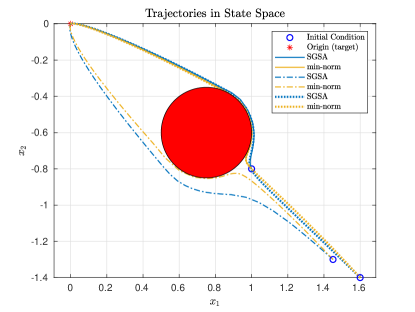
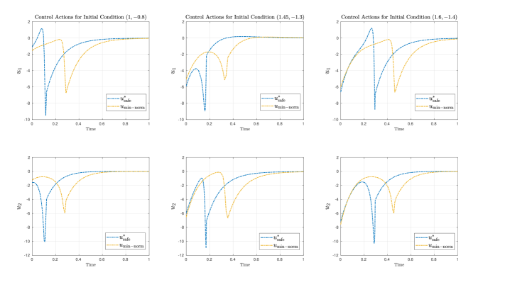
(a)

Figure 1: Closed loop responses of the control system (19) under the control of a $5^{\text{th}}$ order NLQR filtered by a min-norm CBF filter (yellow) and the proposed SGSA control (blue) with different initial conditions. The red circle represents the unsafe region. The proposed method safely stabilizes the system and minimizes the cost as shown in Table I. In addition, it can be seen that the SGSA controller reacts earlier to minimize the cumulative cost and avoid the unsafe region whereas the min-norm controller sticks to the nominal control, NLQR, which results in a sub-optimal behavior.

VII Conclusions and Future Work

We presented an optimal safe control problem for safety-critical control systems that need to be efficiently regulated to minimize a given cost integral while ensuring safety. The proposed work utilized control barrier functions to enforce safety which was used to constraint the solution of the HJB equation. A CBF certified optimal controller was provided. We showed that the proposed controller belongs to the set of controls that renders the system safe and is the one that minimizes the given cost functional. To solve the constrained HJB equation and synthesize the optimal safe control law, a modified Galerkin successive approximation (GSA) algorithm was proposed. The off-line algorithm follows the GSA presented in [24, 25] considering the CBF certified control which resulted in more integrals to be computed. The algorithm was implemented on a multi-input nonlinear system to show its efficacy.

Future directions include extending the work to the min-max problem to compute a robust optimal safe control and improving the efficiency and scalability of the algorithm through polynomial approximation and tensor decomposition.

References

• [1] Franco Blanchini “Set invariance in control” In Automatica 35.11 Elsevier, 1999, pp. 1747–1767
• [2] Yurii Nesterov and Arkadii Nemirovskii “Interior-point polynomial algorithms in convex programming” SIAM, 1994
• [3] Stephen Prajna “Barrier certificates for nonlinear model validation” In 42nd IEEE International Conference on Decision and Control (IEEE Cat. No. 03CH37475) 3, 2003, pp. 2884–2889 IEEE
• [4] Stephen Prajna and Ali Jadbabaie “Safety verification of hybrid systems using barrier certificates” In International Workshop on Hybrid Systems: Computation and Control, 2004, pp. 477–492 Springer
• [5] Peter Wieland and Frank Allgöwer “Constructive safety using control barrier functions” In IFAC Proceedings Volumes 40.12 Elsevier, 2007, pp. 462–467
• [6] Aaron D Ames, Jessy W Grizzle and Paulo Tabuada “Control barrier function based quadratic programs with application to adaptive cruise control” In 53rd IEEE Conference on Decision and Control, 2014, pp. 6271–6278 IEEE
• [7] Muhammad Zakiyullah Romdlony and Bayu Jayawardhana “Uniting control Lyapunov and control barrier functions” In 53rd IEEE Conference on Decision and Control, 2014, pp. 2293–2298 IEEE
• [8] Aaron D Ames, Xiangru Xu, Jessy W Grizzle and Paulo Tabuada “Control barrier function based quadratic programs for safety critical systems” In IEEE Transactions on Automatic Control 62.8 IEEE, 2016, pp. 3861–3876
• [9] Muhammad Zakiyullah Romdlony and Bayu Jayawardhana “Stabilization with guaranteed safety using control Lyapunov–barrier function” In Automatica 66 Elsevier, 2016, pp. 39–47
• [10] Ayush Agrawal and Koushil Sreenath “Discrete Control Barrier Functions for Safety-Critical Control of Discrete Systems with Application to Bipedal Robot Navigation.” In Robotics: Science and Systems, 2017
• [11] Andrew J Taylor and Aaron D Ames “Adaptive safety with control barrier functions” In 2020 American Control Conference (ACC), 2020, pp. 1399–1405 IEEE
• [12] James A Primbs, Vesna Nevistić and John C Doyle “Nonlinear optimal control: A control Lyapunov function and receding horizon perspective” In Asian Journal of Control 1.1 Wiley Online Library, 1999, pp. 14–24
• [13] Yuxiao Chen, Mohamadreza Ahmadi and Aaron D Ames “Optimal safe controller synthesis: A density function approach” In 2020 American Control Conference (ACC), 2020, pp. 5407–5412 IEEE
• [14] Max H Cohen and Calin Belta “Approximate optimal control for safety-critical systems with control barrier functions” In 2020 59th IEEE Conference on Decision and Control (CDC), 2020, pp. 2062–2067 IEEE
• [15] Aaron D Ames et al. “Control barrier functions: Theory and applications” In 2019 18th European Control Conference (ECC), 2019, pp. 3420–3431 IEEE
• [16] Quan Nguyen and Koushil Sreenath “Exponential control barrier functions for enforcing high relative-degree safety-critical constraints” In 2016 American Control Conference (ACC), 2016, pp. 322–328 IEEE
• [17] Wei Xiao and Calin Belta “Control barrier functions for systems with high relative degree” In 2019 IEEE 58th Conference on Decision and Control (CDC), 2019, pp. 474–479 IEEE
• [18] Nader Sadegh and Hassan Almubarak “Recursive Analytic Solution of Nonlinear Optimal Regulators” In submitted for publication
• [19] Frank L Lewis, Draguna Vrabie and Vassilis L Syrmos “Optimal control” John Wiley & Sons, 2012
• [20] Dahlard L Lukes “Optimal regulation of nonlinear dynamical systems” In SIAM Journal on Control 7.1 SIAM, 1969, pp. 75–100
• [21] S Edward Lyshevski “Optimal control of nonlinear continuous-time systems: design of bounded controllers via generalized nonquadratic functionals” In Proceedings of the 1998 American Control Conference. ACC (IEEE Cat. No. 98CH36207) 1, 1998, pp. 205–209 IEEE
• [22] EG Al’Brekht “On the optimal stabilization of nonlinear systems” In Journal of Applied Mathematics and Mechanics 25.5 Elsevier, 1961, pp. 1254–1266
• [23] Hassan K Khalil “Nonlinear systems” Prentice Hall, 2002
• [24] Randal W Beard “Successive Galerkin approximation algorithms for nonlinear optimal and robust control” In International Journal of Control 71.5 Taylor & Francis, 1998, pp. 717–743
• [25] Randal W Beard, George N Saridis and John T Wen “Approximate solutions to the time-invariant Hamilton–Jacobi–Bellman equation” In Journal of Optimization theory and Applications 96.3 Springer, 1998, pp. 589–626
• [26] Clive AJ Fletcher “Computational galerkin methods” In Computational galerkin methods Springer, 1984, pp. 72–85
• [27] Hassan Almubarak, Nader Sadegh and David G. Taylor “Infinite horizon nonlinear quadratic cost regulator” In American Control Conference, 2019. Proceedings of the 2019, 2019 IEEE