Observational constraints on Tsallis modified gravity

Abstract

The thermodynamics-gravity conjecture reveals that one can derive the gravitational field equations by using the first law of thermodynamics and vice versa. Considering the entropy associated with the horizon in the form of non-extensive Tsallis entropy, $S\sim A^{\beta}$ here we first derive the corresponding gravitational field equations by applying the Clausius relation $\delta Q=T\delta S$ to the horizon. We then construct the Friedmann equations of Friedmann-Lemaître-Robertson-Walker (FLRW) universe based on Tsallis modified gravity (TMG). Moreover, in order to constrain the cosmological parameters of TMG model, we use observational data, including Planck cosmic microwave background (CMB), weak lensing, supernovae, baryon acoustic oscillations (BAO), and redshift-space distortions (RSD) data. Numerical results indicate that TMG model with a quintessential dark energy is more compatible with the low redshift measurements of large scale structures by predicting a lower value for the structure growth parameter $\sigma_{8}$ with respect to $\Lambda$CDM model. This implies that TMG model would slightly alleviate the $\sigma_{8}$ tension.

1 Introduction

Considering the discovery of black hole thermodynamics in $1970$ decade (Bardeen et al., 1973; Bekenstein, 1973; Hawking, 1975), it has been known that there is a remarkable analogy between thermodynamics and gravity. Accordingly, there should be some deep relationship between thermodynamics and gravitational field equations, which first disclosed by Jacobson in 1995 (Jacobson, 1995). He derived the covariant form of the Einstein field equations by using the Clausius relation $\delta Q=T\delta S$, together with proportionality of entropy to the horizon area. Jacobson’s investigation reveals that Einstein equations of general relativity is nothing but an equation of state for the spacetime. Also there are more studies in order to explore the profound connection between the theory of general relativity and the laws of thermodynamics (Padmanabhan, 2002, 2005; Eling et al., 2006; Akbar & Cai, 2006; Paranjape et al., 2006; Padmanabhan & Paranjape, 2007; Akbar & Cai, 2007b; Kothawala et al., 2007; Padmanabhan, 2010). Moreover, it is possible to rewrite the Friedmann equations in the form of the first law of thermodynamics at the apparent horizon of FLRW universe and vice versa (Verlinde, 2000; Wang et al., 2001; Frolov & Kofman, 2003; Danielsson, 2005; Cai & Kim, 2005; Bousso, 2005; Akbar & Cai, 2007a; Sheykhi, 2010a). The relationship between gravity and thermodynamics is also considered in the context of braneworld cosmology (Calcagni, 2005; Sheykhi et al., 2007a, b; Sheykhi & Wang, 2009).

Although there are interesting proposals on disclosing the relationship between gravity and thermodynamics, the nature of this deep connection is not clearly explained. To this aim, Verlinde proposed gravity as an entropic force (rather than a fundamental one) caused by a change in the amount of information associated with the positions of material bodies (Verlinde, 2011). Following this holographic scenario, he derived the Newton’s law of gravity and then extended results to relativistic case which yield the Einstein equations. There are more investigations on Verlinde’s entropic force in the literatures (Cai et al., 2010a, b; Myung & Kim, 2010; Sheykhi, 2010b; Banerjee & Majhi, 2010; Cai et al., 2010c; Wei, 2010; Ho et al., 2010; Konoplya, 2010; Kiselev & Timofeev, 2011; Hendi & Sheykhi, 2011b, a; Wei et al., 2011; Sheykhi, 2012; Sheykhi & Teimoori, 2012; Sheykhi & Sarab, 2012). On the other hand, Padmanabhan considered spacetime as an emergent structure (rather than a pre-existing background manifold) in addition to treating field equations as the equations of emergent phenomena (Padmanabhan, 2012). He discussed the spatial expansion of the universe as emergence of space as cosmic time progresses. One can find related explorations on Padmanabhan’s approach in Ref. (Sheykhi et al., 2013b; Tu & Chen, 2013; Ling & Pan, 2013; Eune & Kim, 2013; Sheykhi et al., 2013a; Ai et al., 2013; Tu & Chen, 2015).

In the cosmological setup, it has been shown that one can derive the Friedmann equation of FLRW universe from the first law of thermodynamics $\mathrm{d}E=T\mathrm{d}S+W\mathrm{d}V$ at apparent horizon (Akbar & Cai, 2007a). In this relation, $S$ is the entropy associated with the apparent horizon, which has the same expression as the entropy of the black hole in the background gravity theory. The only change needed is replacing the black hole horizon radius $r_{+}$ with the apparent horizon radius $\tilde{r}_{\mathrm{A}}$ in the entropy associated with the apparent horizon. Accordingly, $T$ is the associated temperature with the apparent horizon, $E$ is the total energy content of the universe and $V$ is the volume inside the apparent horizon, and $W$ is the work density defined as $W=\frac{1}{2}(\rho-p)$, where $\rho$ and $p$ are the energy density and pressure of matter and energy content in the universe, respectively.

The most familiar relation for the black hole entropy is the Bekenstein-Hawking area law entropy (Hawking, 1974, 1975)

$$S_{BH}=\frac{A}{4G}\;,$$ (1)

where $A=4\pi r_{+}^{2}$ is the black hole horizon area. It should be noted that area law of black hole entropy does not always hold. For example, two well-known quantum corrections to the area law are logarithmic (arises from the loop quantum gravity) and power-law (appears in dealing with the entanglement of quantum fields inside and outside the horizon) corrections which have been extensively investigated in the literatures (Rovelli, 1996; Mann & Solodukhin, 1997; Ashtekar et al., 1998; Kaul & Majumdar, 2000; Das et al., 2002, 2008b; Banerjee & Majhi, 2008a, b; Das et al., 2008a; Zhang, 2008; Radicella & Pavón, 2010). On the other hand, it was argued that the Boltzmann-Gibbs (BG) theory is not convincing in divergent partition function systems including large scales gravitational systems (Gibbs, 2010). As a result, the BG additive entropy should be generalized to non-additive (non-extensive) entropy for such systems (Tsallis, 1988; Lyra & Tsallis, 1998; Tsallis et al., 1998; Tsallis, 2011, 2012; da C. Nunes et al., 2014). In this regards, and using the statistical arguments, Tsallis and Cirto argued that the microscopic mathematical expression of the thermodynamical entropy of a black hole does not obey the area law and should be modified as (Tsallis & Cirto, 2013; Sheykhi, 2018)

$$S=\gamma A^{\beta}\;,$$ (2)

where $\gamma$ is a constant, $\beta$ is called the non-extensive or Tsallis parameter, and $A$ is the black hole horizon area. It should be noted that in the limit $\beta\to 1$ the area law entropy expression will be recovered. For more investigations related to Tsallis entropy, refer to e.g. (Sayahian Jahromi et al., 2018; Abdollahi Zadeh et al., 2018; Saridakis et al., 2018; Sadri, 2019; Mamon et al., 2020; Ghoshal & Lambiase, 2021; da Silva & Silva, 2021; Nojiri et al., 2021).

In the context of general relativity, one can derive Einstein field equations by applying the area law entropy (1) in Clausius relation (Eling et al., 2006), which describes the concordance $\Lambda$CDM model. However, in spite of the fact that $\Lambda$CDM model is properly confirmed by current observational data (Percival et al., 2010; Hinshaw et al., 2013), there are some discrepancies between the Planck cosmic microwave background (CMB) data (Aghanim et al., 2020), and low redshift observations, chiefly local measurements of the structure growth parameter $\sigma_{8}$ (Allen et al., 2003), and also local determinations of the Hubble constant $H_{0}$ (Riess et al., 2016, 2018, 2019, 2021). These tensions might indicate some new physics beyond the standard cosmological model. In this direction, we investigate the potentiality of Tsallis modified gravity (TMG) in alleviating the mismatch between local observations and high redshift measurements.

In order to derive the modified Friedmann equations from Tsallis entropy at apparent horizon of FLRW universe, we should consider $A$ in relation (2) as the area of apparent horizon defined as

$$A=4\pi\tilde{r}^{2}_{\mathrm{A}}\;,$$ (3)

where $\tilde{r}_{\mathrm{A}}$ is the apparent horizon radius (Bak & Rey, 2000)

$$\tilde{r}_{\mathrm{A}}=\Big{(}H^{2}+\frac{K}{a^{2}}\Big{)}^{-1/2}\;,$$ (4)

in which $H$ is the Hubble parameter and $K=-1,0,1$ is the curvature constant corresponding to open, flat and closed universe, respectively. Throughout this paper we set $k_{\mathrm{B}}=c=\hbar=1$ for simplicity.

The paper is organized as follows. In section 2, we derive the corresponding field equations as well as the modified Friedmann equations in the context of TMG model. Section 3 is dedicated to numerical solutions of TMG model. In section 4 we constrain our model with observational data. We summarize our results in section 5.

2 Modified gravitational field equations from Tsallis entropy

In this approach, we consider a spatially flat homogeneous and isotropic FLRW universe, described by the following line element in the background level

$$\mathrm{d}s^{2}=a^{2}(\tau)\big{(}-\mathrm{d}\tau^{2}+\mathrm{d}\boldsymbol{x}^{2}\big{)}\;,$$ (5)

where $\tau$ is the conformal time. Moreover, we are interested in scalar perturbations to linear order, so following Ref. (Ma & Bertschinger, 1995), the perturbed metric in conformal Newtonian gauge is

$$\mathrm{d}s^{2}=a^{2}(\tau)\Big{(}-\big{(}1+2\Psi\big{)}\mathrm{d}\tau^{2}+\big{(}1-2\Phi\big{)}\mathrm{d}\boldsymbol{x}^{2}\Big{)}\;,$$ (6)

where $\Psi$ and $\Phi$ are gravitational potentials. Also in synchronous gauge we have

$$\mathrm{d}s^{2}=a^{2}(\tau)\Big{(}-\mathrm{d}\tau^{2}+\big{(}\delta_{ij}+h_{ij}\big{)}\mathrm{d}x^{i}\mathrm{d}x^{j}\Big{)}\;,$$ (7)

in which $h_{ij}=\mathrm{diag}(-2\eta,-2\eta,h+4\eta)$, with scalar perturbations $h$ and $\eta$. We assume the matter and energy content of the universe as a perfect fluid with the following energy-momentum tensor

$$T_{\mu\nu}=\big{(}\rho+p\big{)}u_{\mu}u_{\nu}+g_{\mu\nu}p\;,$$ (8)

where $\rho=\bar{\rho}+\delta\rho$ is the energy density, $p=\bar{p}+\delta p$ is the pressure, and $u_{\mu}$ is the four-velocity (and a bar indicates the background level).

In order to derive Einstein field equations from Tsallis entropy, we apply the Clausius relation

$$\delta Q=T\delta S\;.$$ (9)

It is assumed that the Clausius relation is satisfied on a local causal horizon $\mathcal{H}$ (which here it is the apparent horizon).

Let us now consider equation (9) more specifically. The associated temperature with the apparent horizon is given by

$$T=\frac{\kappa}{2\pi}\;,$$ (10)

where $\kappa$ is the surface gravity at apparent horizon. Also, according to equation (2), $\delta S$ can be written as

$$\delta S=\gamma\beta A^{\beta-1}\delta A\;.$$ (11)

In order to define $\delta Q$, we follow the approach of Ref. (Jacobson, 1995; Eling et al., 2006) which reads

$$\delta Q=-\kappa\int_{\mathcal{H}}\lambda T_{\mu\nu}k^{\mu}k^{\nu}\mathrm{d}\lambda\mathrm{d}A\;,$$ (12)

and also we have

$$\delta A=\int_{\mathcal{H}}\theta\mathrm{d}\lambda\mathrm{d}A\;,$$ (13)

$$\theta=-\lambda R_{\mu\nu}k^{\mu}k^{\nu}\;.$$ (14)

Substituting relations (10),(11) and (12) in equation (9) would result in

$$\kappa\int_{\mathcal{H}}(-\lambda)T_{\mu\nu}k^{\mu}k^{\nu}\mathrm{d}\lambda\mathrm{d}A$$

$$=\frac{\kappa}{2\pi}\gamma\beta\int_{\mathcal{H}}(-\lambda)R_{\mu\nu}k^{\mu}k^{\nu}A^{\beta-1}\mathrm{d}\lambda\mathrm{d}A\;,$$ (15)

$$\to\int_{\mathcal{H}}(-\lambda)\bigg{(}-2\pi T_{\mu\nu}+\gamma\beta R_{\mu\nu}A^{\beta-1}\bigg{)}k^{\mu}k^{\nu}\mathrm{d}\lambda\mathrm{d}A=0\;.$$ (16)

So for all null $k^{\mu}$ we should have

$$-2\pi T_{\mu\nu}+\gamma\beta R_{\mu\nu}A^{\beta-1}=fg_{\mu\nu}\;,$$ (17)

in which $f$ is a scalar. Then, the energy-momentum conservation ($\nabla^{\mu}T_{\mu\nu}=0$) would impose

$$\nabla^{\mu}\big{(}\gamma\beta R_{\mu\nu}A^{\beta-1}-fg_{\mu\nu}\big{)}=0\;,$$ (18)

which after doing some calculations results in

$$\frac{1}{2}\gamma\beta\big{(}\partial_{\nu}R\big{)}A^{\beta-1}+\gamma\beta R_{\mu\nu}\partial^{\mu}A^{\beta-1}=\partial_{\nu}f\,.$$ (19)

However, the LHS of equation (19) is not the gradient of a scalar. It reveals that the Clausius relation does not hold due to non-equilibrium thermodynamics. Hence, in order to resolve this contradiction, we use the entropy balance relation (Eling et al., 2006)

$$\delta S=\frac{\delta Q}{T}+\mathrm{d}_{i}S\;,$$ (20)

where $\mathrm{d}_{i}S$ is the entropy produced inside the system due to irreversible processes (De Groot & Mazur, 1962). In order to restore the energy-momentum conservation, we choose $\mathrm{d}_{i}S$ as

$$\mathrm{d}_{i}S=\gamma\beta\int_{\mathcal{H}}(-\lambda)\nabla_{\mu}\nabla_{\nu}A^{\beta-1}k^{\mu}k^{\nu}\mathrm{d}\lambda\mathrm{d}A\;.$$ (21)

Thus, equation (20) reads

$$\gamma\beta\int_{\mathcal{H}}(-\lambda)R_{\mu\nu}k^{\mu}k^{\nu}A^{\beta-1}\mathrm{d}\lambda\mathrm{d}A$$

$$=2\pi\int_{\mathcal{H}}(-\lambda)T_{\mu\nu}k^{\mu}k^{\nu}\mathrm{d}\lambda\mathrm{d}A$$

$$+\gamma\beta\int_{\mathcal{H}}(-\lambda)\nabla_{\mu}\nabla_{\nu}A^{\beta-1}k^{\mu}k^{\nu}\mathrm{d}\lambda\mathrm{d}A\,,$$ (22)

$$\to\int_{\mathcal{H}} (-\lambda)\bigg{(}\gamma\beta R_{\mu\nu}A^{\beta-1}-2\pi T_{\mu\nu}-\gamma\beta\nabla_{\mu}\nabla_{\nu}A^{\beta-1}\bigg{)}$$

$$\times k^{\mu}k^{\nu}\mathrm{d}\lambda\mathrm{d}A=0\;.$$ (23)

Likewise, for all null $k^{\mu}$ we obtain

$$\gamma\beta R_{\mu\nu}A^{\beta-1}-2\pi T_{\mu\nu}-\gamma\beta\nabla_{\mu}\nabla_{\nu}A^{\beta-1}=fg_{\mu\nu}\;.$$ (24)

According to the energy-momentum conservation, we should have

$$\nabla^{\mu}\big{(}\gamma\beta R_{\mu\nu}A^{\beta-1}-\gamma\beta\nabla_{\mu}\nabla_{\nu}A^{\beta-1}-fg_{\mu\nu}\big{)}=0\,.$$ (25)

Then, considering $\nabla^{\mu}\nabla_{\mu}\nabla_{\nu}A^{\beta-1}=\nabla_{\nu}\Box A^{\beta-1}+R_{\zeta\nu}\partial^{\zeta}A^{\beta-1}$, we get

$$\gamma\beta\Big{(}\frac{1}{2}\big{(}\partial_{\nu}R\big{)}A^{\beta-1}-\partial_{\nu}\Box A^{\beta-1}\Big{)}=\partial_{\nu}f\;.$$ (26)

It is possible to define the scalar $\mathcal{L}$ as $\mathcal{L}=RA^{\beta-1}$, which results in

$$\frac{\partial\mathcal{L}}{\partial R}=A^{\beta-1}\;,$$

$$\partial_{\nu}R=\frac{\partial R}{\partial x^{\nu}}=\frac{\partial R}{\partial\mathcal{L}}\frac{\partial\mathcal{L}}{\partial x^{\nu}}=A^{1-\beta}\partial_{\nu}\mathcal{L}\;,$$

$$\to\big{(}\partial_{\nu}R\big{)}A^{\beta-1}=\partial_{\nu}\mathcal{L}\;.$$ (27)

Thus equation (26) takes the form

$$\gamma\beta\Big{(}\frac{1}{2}\partial_{\nu}\mathcal{L}-\partial_{\nu}\Box A^{\beta-1}\Big{)}=\partial_{\nu}f\;,$$ (28)

which results in the following equation for the scalar $f$

$$f =\gamma\beta\Big{(}\frac{1}{2}\mathcal{L}-\Box A^{\beta-1}\Big{)}$$

$$=\gamma\beta\Big{(}\frac{1}{2}RA^{\beta-1}-\Box A^{\beta-1}\Big{)}\;.$$ (29)

Therefore, the gravitational field equations based on nonextensive Tsallis entropy (2) take the following form

$$R_{\mu\nu}A^{\beta-1}-\nabla_{\mu}\nabla_{\nu}A^{\beta-1}-\frac{1}{2}RA^{\beta-1}g_{\mu\nu}+\Box A^{\beta-1}g_{\mu\nu}$$

$$=\frac{2\pi}{\gamma\beta}T_{\mu\nu}\;.$$ (30)

Equation (2) is indeed the modified Einstein field equations, when the entropy associated with the horizon does not obey the area law and instead is given by equation (2). When $\beta=1$, equation (2) restores the standard Einstein equations. Given the modified Einstein equations at hand, we are in the position to derive the corresponding modified Friedmann equations in the background of a flat FLRW universe. According to relations (3) and (4), for a spatially flat universe we have

$$A^{\beta-1}=(4\pi)^{\beta-1}\Big{(}\frac{a^{\prime}}{a^{2}}\Big{)}^{2-2\beta}=(4\pi)^{\beta-1}H^{2-2\beta}\;,$$ (31)

where a prime indicates a deviation with respect to the conformal time, and $H={a^{\prime}}/{a^{2}}$ is the Hubble parameter. The $(00)$ and $(ii)$ components of the modified field equations (2) in a background level are given by

$$\Big{(}\frac{a^{\prime}}{a^{2}}\Big{)}^{2-2\beta}\Bigg{\{}\Big{(}\frac{a^{\prime}}{a}\Big{)}^{2}+2\big{(}1-\beta\big{)}\bigg{(}\frac{a^{\prime\prime}}{a}-2\Big{(}\frac{a^{\prime}}{a}\Big{)}^{2}\bigg{)}\Bigg{\}}$$

$$=\frac{8\pi G}{3}a^{2}\sum_{i}\bar{\rho}_{i}\;,$$ (32)

$$\Big{(}\frac{a^{\prime}}{a^{2}}\Big{)}^{2-2\beta}\Bigg{\{}-2\frac{a^{\prime\prime}}{a}+\Big{(}\frac{a^{\prime}}{a}\Big{)}^{2}+2\big{(}1-\beta\big{)}\Bigg{[}5\frac{a^{\prime\prime}}{a}-4\Big{(}\frac{a^{\prime}}{a}\Big{)}^{2}$$

$$-\frac{a^{\prime\prime\prime}}{a^{\prime}}-\big{(}1-2\beta\big{)}\bigg{(}\frac{a^{\prime\prime}}{a^{\prime}}-2\frac{a^{\prime}}{a}\bigg{)}^{2}\Bigg{]}\Bigg{\}}=8\pi Ga^{2}\sum_{i}\bar{p}_{i}\;,$$ (33)

where we have taken the energy momentum tensor $T_{\mu\nu}$ as defined in equation (8), and also we have defined $\gamma={(4\pi)^{1-\beta}}/{(4G\beta)}$. Here $i$ indicates the component $i^{th}$ of the energy in the universe. In terms of the Hubble parameter $H$, the above equations can be written as

$$H^{4-2\beta}+2\big{(}1-\beta\big{)}H^{2-2\beta}H^{\prime}\frac{1}{a}=\frac{8\pi G}{3}\sum_{i}\bar{\rho}_{i}\;,$$ (34)

$$H^{2-2\beta}\Bigg{\{}2\big{(}\beta-2\big{)}H^{\prime}\frac{1}{a}-3H^{2}$$

$$-2\big{(}1-\beta\big{)}\bigg{(}\big{(}1-2\beta\big{)}\frac{H^{\prime 2}}{H^{2}}+\frac{H^{\prime\prime}}{H}\bigg{)}\frac{1}{a^{2}}\Bigg{\}}=8\pi G\sum_{i}\bar{p}_{i}\;.$$ (35)

Combining equations (34) and (2), one can rewrite the first modified Friedmann equation as

$$H^{4-2\beta}=\frac{1}{4\beta-3}\frac{8\pi G}{3}\sum_{i}\bar{\rho}_{i}\;.$$ (36)

Taking into account the definition of the total density parameter $\Omega_{\mathrm{tot}}={\bar{\rho}}/{\rho_{\mathrm{cr}}}$, where $\rho_{\mathrm{cr}}={3H^{2}}/{(8\pi G)}$ and $\bar{\rho}=\sum_{i}\bar{\rho}_{i}$, we can further rewrite equation (36) in the form

$$\Omega_{\mathrm{tot}}=\big{(}4\beta-3\big{)}H^{2-2\beta}\;,$$ (37)

which differs from the standard cosmology, unless for the case $\beta=1$ where we have $\Omega_{\mathrm{tot}}=1$.

It should be noted that in this model $\rho_{\mathrm{tot}}$ includes radiation (R), matter (M) (dark matter (DM) and baryons (B)) and the fluid "f" with a constant equation of state $w_{\mathrm{f}}={\bar{p}_{\mathrm{f}}}/{\bar{\rho}_{\mathrm{f}}}$. Considering the total equation of state $w_{\mathrm{tot}}={\bar{p}_{\mathrm{tot}}}/{\bar{\rho}_{\mathrm{tot}}}$, under the condition $w_{\mathrm{tot}}<({1-2\beta})/{3}$, the universe would experience an accelerated expansion. Choosing $\beta=1$, results in $w_{\mathrm{tot}}<-{1}/{3}$ which is the condition for an accelerated universe in standard cosmology. However, different values of Tsallis parameter $\beta$, can result in different conditions from general relativity. In particular, considering $\beta\geq 1/2$ would result in $w_{\mathrm{tot}}<0$, while for $\beta<1/2$, $w_{\mathrm{tot}}$ can take positive value and we still have the late-time acceleration of the cosmic expansion. For example, by choosing $\beta=1/3$ we obtain $w_{\mathrm{tot}}<1/9$. This implies that one may consider a universe filled with baryonic matter, and still enjoys an accelerated expansion without invoking any dark companion for its matter/energy content. This is consistent with the argument given in (Sheykhi, 2020).

Moreover, modified field equations to linear order of perturbations in conformal Newtonian gauge (con) take the form

$$\Big{(}\frac{a^{\prime}}{a^{2}}\Big{)}^{2-2\beta}\Bigg{\{}3\frac{a^{\prime}}{a}\Phi^{\prime}+k^{2}\Phi+3\Big{(}\frac{a^{\prime}}{a}\Big{)}^{2}\Psi$$

$$+3\big{(}1-\beta\big{)}\bigg{(}\frac{a^{\prime\prime}}{a^{\prime}}-2\frac{a^{\prime}}{a}\bigg{)}\bigg{(}\Phi^{\prime}+2\Psi\frac{a^{\prime}}{a}\bigg{)}\Bigg{\}}$$

$$=-4\pi Ga^{2}\sum_{i}\delta\rho_{i(\mathrm{con})}\;,$$ (38)

$$\Big{(}\frac{a^{\prime}}{a^{2}}\Big{)}^{2-2\beta}\Bigg{\{}k^{2}\Phi^{\prime}+\frac{a^{\prime}}{a}k^{2}\Psi+\big{(}1-\beta\big{)}\bigg{(}\frac{a^{\prime\prime}}{a^{\prime}}-2\frac{a^{\prime}}{a}\bigg{)}k^{2}\Psi\Bigg{\}}$$

$$=4\pi Ga^{2}\sum_{i}\big{(}\bar{\rho}_{i}+\bar{p}_{i}\big{)}\theta_{i(\mathrm{con})}\;,$$ (39)

$$\Phi=\Psi\;,$$ (40)

$$\Big{(}\frac{a^{\prime}}{a^{2}}\Big{)}^{2-2\beta}\Bigg{\{}2\frac{a^{\prime\prime}}{a}\Psi-\Big{(}\frac{a^{\prime}}{a}\Big{)}^{2}\Psi+\frac{a^{\prime}}{a}\Psi^{\prime}+2\frac{a^{\prime}}{a}\Phi^{\prime}+\Phi^{\prime\prime}$$

$$+\frac{k^{2}}{3}\big{(}\Phi-\Psi\big{)}+\big{(}1-\beta\big{)}\Bigg{\{}2\bigg{(}\frac{a^{\prime\prime}}{a^{\prime}}-2\frac{a^{\prime}}{a}\bigg{)}\bigg{(}2\frac{a^{\prime}}{a}\Psi+\Phi^{\prime}\bigg{)}$$

$$+2\Psi\Bigg{[}\big{(}1-2\beta\big{)}\bigg{(}\frac{a^{\prime\prime}}{a^{\prime}}-2\frac{a^{\prime}}{a}\bigg{)}^{2}+\frac{a^{\prime\prime\prime}}{a^{\prime}}-7\frac{a^{\prime\prime}}{a}+8\Big{(}\frac{a^{\prime}}{a}\Big{)}^{2}\Bigg{]}$$

$$+\Psi^{\prime}\bigg{(}\frac{a^{\prime\prime}}{a^{\prime}}-2\frac{a^{\prime}}{a}\bigg{)}\Bigg{\}}\Bigg{\}}=4\pi Ga^{2}\sum_{i}\delta p_{i(\mathrm{con})}\;.$$ (41)

Also in synchronous gauge (syn) we have

$$\Big{(}\frac{a^{\prime}}{a^{2}}\Big{)}^{2-2\beta}\Bigg{\{}\frac{a^{\prime}}{a}h^{\prime}-2k^{2}\eta+\big{(}1-\beta\big{)}h^{\prime}\bigg{(}\frac{a^{\prime\prime}}{a^{\prime}}-2\frac{a^{\prime}}{a}\bigg{)}\Bigg{\}}$$

$$=8\pi Ga^{2}\sum_{i}\delta\rho_{i(\mathrm{syn})}\;,$$ (42)

$$\Big{(}\frac{a^{\prime}}{a^{2}}\Big{)}^{2-2\beta}k^{2}\eta^{\prime}=4\pi Ga^{2}\sum_{i}\big{(}\bar{\rho}_{i}+\bar{p}_{i}\big{)}\theta_{i(\mathrm{syn})}\;,$$ (43)

$$\Big{(}\frac{a^{\prime}}{a^{2}}\Big{)}^{2-2\beta}\Bigg{\{}\frac{1}{2}h^{\prime\prime}+3\eta^{\prime\prime}+\frac{a^{\prime}}{a}h^{\prime}+6\frac{a^{\prime}}{a}\eta^{\prime}-k^{2}\eta$$

$$+2\big{(}1-\beta\big{)}\bigg{(}\frac{a^{\prime\prime}}{a^{\prime}}-2\frac{a^{\prime}}{a}\bigg{)}\bigg{(}\frac{1}{2}h^{\prime}+3\eta^{\prime}\bigg{)}\Bigg{\}}=0\;,$$ (44)

$$\Big{(}\frac{a^{\prime}}{a^{2}}\Big{)}^{2-2\beta}\Bigg{\{}-2\frac{a^{\prime}}{a}h^{\prime}-h^{\prime\prime}+2k^{2}\eta$$

$$-2\big{(}1-\beta\big{)}\bigg{(}\frac{a^{\prime\prime}}{a^{\prime}}-2\frac{a^{\prime}}{a}\bigg{)}h^{\prime}\Bigg{\}}=24\pi Ga^{2}\sum_{i}\delta p_{i(\mathrm{syn})}\;.$$ (45)

It can be easily seen that for $\beta=1$, the standard field equations in Einstein gravity will be restored. In the following we study TMG model in synchronous gauge.

Furthermore, the conservation equations in TMG model are the same as those in general relativity, so for the matter and the fluid components we find the following conservation equations in the synchronous gauge

$$\delta^{\prime}_{\mathrm{M(syn)}}=-\theta_{\mathrm{M(syn)}}-\frac{1}{2}h^{\prime}\;,$$ (46)

$$\theta^{\prime}_{\mathrm{M(syn)}}=-\frac{a^{\prime}}{a}\theta_{\mathrm{M(syn)}}\;,$$ (47)

$$\delta^{\prime}_{\mathrm{f(syn)}}=-3\frac{a^{\prime}}{a}\big{(}c^{2}_{s,\mathrm{f}}-w_{\mathrm{f}}\big{)}\delta_{\mathrm{f(syn)}}-\frac{1}{2}h^{\prime}\big{(}1+w_{\mathrm{f}}\big{)}$$

$$-\big{(}1+w_{\mathrm{f}}\big{)}\bigg{(}1+9\Big{(}\frac{a^{\prime}}{a}\Big{)}^{2}\big{(}c^{2}_{s,\mathrm{f}}-c^{2}_{a,\mathrm{f}}\big{)}\frac{1}{k^{2}}\bigg{)}\theta_{\mathrm{f(syn)}}\;,$$ (48)

$$\theta^{\prime}_{\mathrm{f(syn)}}=\frac{a^{\prime}}{a}\big{(}3c^{2}_{s,\mathrm{f}}-1\big{)}\theta_{\mathrm{f(syn)}}+\frac{k^{2}c^{2}_{s,\mathrm{f}}}{1+w_{\mathrm{f}}}\delta_{\mathrm{f(syn)}}\;.$$ (49)

In order to understand the properties of TMG model more precisely and also constrain the Tsallis parameter $\beta$ with observational data, we modify the Boltzmann code Cosmic Linear Anisotropy Solving System (CLASS) (Blas et al., 2011) according to this model. Furthermore, running a Markov Chain Monte Carlo (MCMC) analysis through the Monte Python code (Audren et al., 2013; Brinckmann & Lesgourgues, 2018), provides us with constraints on the cosmological parameters.

3 Numerical results

In this part, we study TMG model by implementing modified field equations in the CLASS code. Accordingly, we use Planck 2018 data (Aghanim et al., 2020) for the cosmological parameters given by $\Omega_{\mathrm{B},0}h^{2}=0.02242$, $\Omega_{\mathrm{DM},0}h^{2}=0.11933$, $H_{0}=67.66\,\mathrm{km\,s^{-1}\,Mpc^{-1}}$, $A_{s}=2.105\times 10^{-9}$, and $\tau_{\mathrm{reio}}=0.0561$. Since the nature of fluid is unknown to us, without loss of generality we can consider $w_{\mathrm{f}}=-0.98$ and $c_{s,\mathrm{f}}^{2}=1$.

The CMB temperature anisotropy and matter power spectra diagrams are shown in Fig. 1.

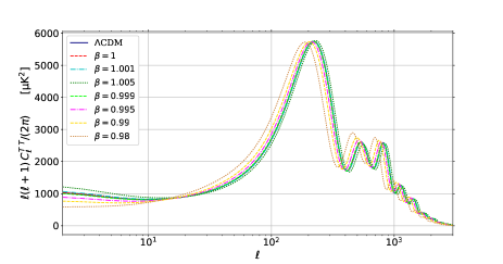
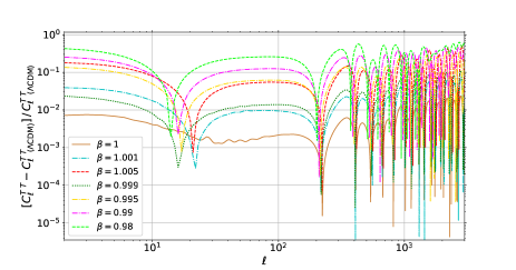
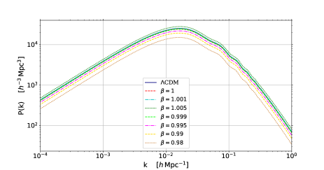
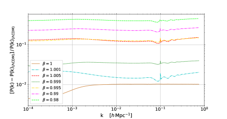
Figure 1: The CMB power spectra (upper left) and their relative ratio with respect to the standard model (upper right) for different values of $\beta$. Lower panels show the analogous diagrams for the matter power spectrum.

According to matter power spectra diagrams, there is a decrease in structure growth for TMG model with $\beta<1$. So regarding discrepancies between low redshift observational data and CMB results, it can be concluded that TMG model with $\beta<1$ is more consistent with local measurements of the structure growth parameter $\sigma_{8}$. This feature of TMG model can be also understood from matter density contrast diagrams in Fig. 2.

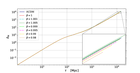
Figure 2: Matter density contrast diagrams in term of conformal time for TMG model with different values of $\beta$ compared to $\Lambda$CDM.

It is also interesting to investigate the evolution of the Hubble parameter in TMG model which is described in equation (36). Considering the evolution of Hubble parameter illustrated in Fig. 3, it can be understood that choosing $\beta>1$ would increase the current value of Hubble parameter, which is consequently more compatible with local determinations of this parameter. However, the $H_{0}$ tension problem becomes more severe for $\beta<1$.

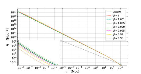
Figure 3: Hubble parameter in term of conformal time for TMG model with different values of $\beta$ compared to $\Lambda$CDM.

4 Observational constraints

In order to explore constraints on cosmological parameters of TMG model, we run an MCMC analysis using the Monte Python code (Audren et al., 2013; Brinckmann & Lesgourgues, 2018). The following set of parameters is considered in the MCMC analysis:
{$100\,\Omega_{\mathrm{B},0}h^{2}$, $\Omega_{\mathrm{DM},0}h^{2}$, $100\,\theta_{s}$, $\ln(10^{10}A_{s})$, $n_{s}$, $\tau_{\mathrm{reio}}$, $w_{\mathrm{f}}$, $\beta$},
where $\Omega_{\mathrm{B},0}h^{2}$ and $\Omega_{\mathrm{DM},0}h^{2}$ are the baryon and cold dark matter densities relative to the critical density respectively, $\theta_{s}$ is the ratio of the sound horizon to the angular diameter distance at decoupling, $A_{s}$ is the amplitude of the primordial scalar perturbation spectrum, $n_{s}$ is the scalar spectral index, $\tau_{\mathrm{reio}}$ is the optical depth to reionization, $w_{\mathrm{f}}$ is the fluid equation of state parameter, and $\beta$ is the Tsallis parameter. Furthermore, we have four derived parameters which are the reionization redshift ($z_{\mathrm{reio}}$), the matter density parameter ($\Omega_{\mathrm{M},0}$), the Hubble constant ($H_{0}$), and the root-mean-square mass fluctuations on scales of 8 $h^{-1}$ Mpc ($\sigma_{8}$). According to preliminary numerical works, we consider the prior range [$0.98$, $1.008$] for the Tsallis parameter, and also we set no prior range on the fluid equation of state parameter $w_{\mathrm{f}}$.

In this analysis we use six likelihoods: The Planck likelihood with Planck 2018 data (containing high-$l$ TT,TE,EE, low-$l$ EE, low-$l$ TT, and lensing) (Aghanim et al., 2020), the Planck-SZ likelihood for the Sunyaev-Zeldovich effect measured by Planck (Ade et al., 2016, 2014), the CFHTLenS likelihood with the weak lensing data (Kilbinger et al., 2013; Heymans et al., 2013), the Pantheon likelihood with the supernovae data (Scolnic et al., 2018), the BAO likelihood with the baryon acoustic oscillations (BAO) data (Beutler et al., 2011; Anderson et al., 2014), and the BAORSD likelihood for BAO and redshift-space distortions (RSD) measurements (Alam et al., 2017; Buen-Abad et al., 2018).

Constraints on the cosmological parameters, considering the combined "Planck + Planck-SZ + CFHTLenS + Pantheon + BAO + BAORSD" data set, are displayed in Table 1.

Table 1: Best fit values and 68% and 95% confidence limits for cosmological parameters from "Planck + Planck-SZ + CFHTLenS + Pantheon + BAO + BAORSD" data set for $\Lambda$CDM and TMG model.

	$\Lambda$CDM		TMG model
parameter	best fit	68% & 95% limits	best fit	68% & 95% limits
$100\,\Omega_{\mathrm{B},0}h^{2}$	$2.261$	$2.263^{+0.012+0.026}_{-0.013-0.025}$	$2.272$	$2.268^{+0.014+0.027}_{-0.015-0.028}$
$\Omega_{\mathrm{DM},0}h^{2}$	$0.1163$	$0.1164^{+0.00078+0.0015}_{-0.00079-0.0015}$	$0.1166$	$0.1160^{+0.00097+0.0016}_{-0.00077-0.0017}$
$100\,\theta_{s}$	$1.042$	$1.042^{+0.00029+0.00055}_{-0.00026-0.00053}$	$1.042$	$1.042^{+0.00026+0.00054}_{-0.00028-0.00052}$
$\ln(10^{10}A_{s})$	$3.034$	$3.024^{+0.010+0.023}_{-0.014-0.021}$	$3.026$	$3.028^{+0.011+0.024}_{-0.014-0.025}$
$n_{s}$	$0.9712$	$0.9719^{+0.0036+0.0072}_{-0.0039-0.0074}$	$0.9706$	$0.9720^{+0.0038+0.0074}_{-0.0040-0.0076}$
$\tau_{\mathrm{reio}}$	$0.05358$	$0.04963^{+0.0041+0.010}_{-0.0074-0.0096}$	$0.05102$	$0.05158^{+0.0059+0.011}_{-0.0072-0.012}$
$w_{\mathrm{f}}$	—	—	$-0.9677$	$-0.9944^{+0.041+0.089}_{-0.046-0.084}$
$\beta$	—	—	$0.9999$	$0.9997^{+0.00047+0.00098}_{-0.00048-0.00090}$
$z_{\mathrm{reio}}$	$7.502$	$7.084^{+0.50+1.0}_{-0.69-1.0}$	$7.231$	$7.275^{+0.59+1.2}_{-0.72-1.2}$
$\Omega_{\mathrm{M},0}$	$0.2871$	$0.2876^{+0.0043+0.0086}_{-0.0044-0.0086}$	$0.2994$	$0.2945^{+0.0076+0.016}_{-0.0074-0.015}$
$H_{0}\;[\mathrm{km\,s^{-1}\,Mpc^{-1}}]$	$69.56$	$69.54^{+0.37+0.73}_{-0.36-0.71}$	$68.20$	$68.62^{+0.79+1.7}_{-0.89-1.8}$
$\sigma_{8}$	$0.8079$	$0.8044^{+0.0045+0.0096}_{-0.0051-0.0091}$	$0.7927$	$0.7956^{+0.0097+0.019}_{-0.0092-0.019}$

The triangle plot for selected cosmological parameters of TMG model is illustrated in Fig. 4.

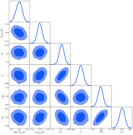
Figure 4: The one-dimensional posterior distribution and two-dimensional posterior contours with 68% and 95% confidence limits from the "Planck + Planck-SZ + CFHTLenS + Pantheon + BAO + BAORSD" data set, for the selected cosmological parameters of TMG model.

According to our results, TMG model predicts a lower value for the structure growth parameter $\sigma_{8}$ with respect to $\Lambda$CDM model. So it seems that TMG model is more compatible with local measurements of structure growth, with a slight alleviation of $\sigma_{8}$ tension. Also the derived best fit value of $w_{\mathrm{f}}$ indicates that the fluid "f" has a negative pressure, and so we can conclude that it is a dark energy fluid. Interestingly enough, the best fit and the mean value of the fluid equation of state parameter demonstrate the quintessential character of dark energy, which is also effective in reducing the growth of structure. However, the phantom nature of $w_{\mathrm{f}}$ is also permitted within the $1\sigma$ confidence level, where $-1.040<w_{\mathrm{f}}<-0.9532$. Moreover, according to the correlation between $\sigma_{8}$ and $H_{0}$, one can conclude that TMG model is not capable of providing a full reconciliation between low redshift probes and CMB measurements.

Furthermore, in order to understand which model provides a better fit to observational data, one can use the Akaike information criterion (AIC) defined as (Akaike, 1974; Burnham & Anderson, 2002)

$$\mathrm{AIC}=-2\ln{\mathcal{L}_{\mathrm{max}}}+2K,$$ (50)

in which $\mathcal{L}_{\mathrm{max}}$ is the maximum likelihood function, and $K$ is the number of free parameters. According to numerical analysis we have $\mathrm{AIC_{(\Lambda CDM)}}=3847.12$ and $\mathrm{AIC_{(TMG)}}=3850.84$, which results in $\Delta\mathrm{AIC}=3.72$. So it can be concluded that the $\Lambda$CDM model is more supported by observational data, while the TMG model can not be ruled out.

5 Conclusions

According to the analogy between thermodynamics and gravity, one can rewrite the Friedmann equation of FLRW universe in the form of the first law of thermodynamics at apparent horizon and vice versa. On the other hand, the Boltzmann-Gibbs (BG) theory is not convincing in gravitational systems which leads us to choose non-additive entropy to study such systems. In the present paper, we have considered the non-additive Tsallis entropy expression at apparent horizon of FLRW universe, to disclose its novel features on cosmological parameters. Accordingly we have derived the gravitational field equations when the entropy associated with the horizon is in the form of Tsallis entropy given in equation (2). In the cosmological background the obtained TMG leads to modified Friedmann equations describing the evolution of the universe. Employing numerical analysis, we constrain the cosmological parameters of this model with observational data, based on Planck CMB, weak lensing, supernovae, BAO, and RSD data. The obtained results indicate that the preferred value of $\sigma_{8}$ in TMG model is lower than the one in $\Lambda$CDM, and so TMG model with a quintessential dark energy can slightly reduce the well known tension between the Planck CMB and local observations of $\sigma_{8}$.

Data availability

No new data were generated or analysed in support of this research.

References

- Abdollahi Zadeh et al. (2018) Abdollahi Zadeh M., Sheykhi A., Moradpour H., Bamba K., 2018, The European Physical Journal C, 78, 940
- Ade et al. (2014) Ade P. A. R., et al., 2014, Astronomy & Astrophysics, 571, A20
- Ade et al. (2016) Ade P. A. R., et al., 2016, Astronomy & Astrophysics, 594, A24
- Aghanim et al. (2020) Aghanim N., et al., 2020, Astronomy & Astrophysics, 641, A6
- Ai et al. (2013) Ai W.-Y., Hu X.-R., Chen H., Deng J.-B., 2013, Phys. Rev. D, 88, 084019
- Akaike (1974) Akaike H., 1974, IEEE Transactions on Automatic Control, 19, 716
- Akbar & Cai (2006) Akbar M., Cai R.-G., 2006, Physics Letters B, 635, 7
- Akbar & Cai (2007a) Akbar M., Cai R.-G., 2007a, Phys. Rev. D, 75, 084003
- Akbar & Cai (2007b) Akbar M., Cai R.-G., 2007b, Physics Letters B, 648, 243
- Alam et al. (2017) Alam S., et al., 2017, Monthly Notices of the Royal Astronomical Society, 470, 2617
- Allen et al. (2003) Allen S. W., Schmidt R. W., Fabian A. C., Ebeling H., 2003, Monthly Notices of the Royal Astronomical Society, 342, 287
- Anderson et al. (2014) Anderson L., et al., 2014, Monthly Notices of the Royal Astronomical Society, 441, 24
- Ashtekar et al. (1998) Ashtekar A., Baez J., Corichi A., Krasnov K., 1998, Phys. Rev. Lett., 80, 904
- Audren et al. (2013) Audren B., Lesgourgues J., Benabed K., Prunet S., 2013, JCAP, 1302, 001
- Bak & Rey (2000) Bak D., Rey S.-J., 2000, Classical and Quantum Gravity, 17, L83
- Banerjee & Majhi (2008a) Banerjee R., Majhi B. R., 2008a, Physics Letters B, 662, 62
- Banerjee & Majhi (2008b) Banerjee R., Majhi B. R., 2008b, Journal of High Energy Physics, 2008, 095
- Banerjee & Majhi (2010) Banerjee R., Majhi B. R., 2010, Phys. Rev. D, 81, 124006
- Bardeen et al. (1973) Bardeen J. M., Carter B., Hawking S. W., 1973, Comm. Math. Phys., 31, 161
- Bekenstein (1973) Bekenstein J. D., 1973, Phys. Rev. D, 7, 2333
- Beutler et al. (2011) Beutler F., et al., 2011, Monthly Notices of the Royal Astronomical Society, 416, 3017
- Blas et al. (2011) Blas D., Lesgourgues J., Tram T., 2011, Journal of Cosmology and Astroparticle Physics, 2011, 034
- Bousso (2005) Bousso R., 2005, Phys. Rev. D, 71, 064024
- Brinckmann & Lesgourgues (2018) Brinckmann T., Lesgourgues J., 2018, MontePython 3: boosted MCMC sampler and other features (arXiv:1804.07261)
- Buen-Abad et al. (2018) Buen-Abad M. A., Schmaltz M., Lesgourgues J., Brinckmann T., 2018, JCAP, 1801, 008
- Burnham & Anderson (2002) Burnham K., Anderson D., 2002, Model Selection and Multimodel Inference: A Practical Information-Theoretic Approach. Springer Verlag
- Cai & Kim (2005) Cai R.-G., Kim S. P., 2005, Journal of High Energy Physics, 2005, 050
- Cai et al. (2010a) Cai R.-G., Cao L.-M., Ohta N., 2010a, Phys. Rev. D, 81, 061501
- Cai et al. (2010b) Cai R.-G., Cao L.-M., Ohta N., 2010b, Phys. Rev. D, 81, 084012
- Cai et al. (2010c) Cai Y.-F., Liu J., Li H., 2010c, Physics Letters B, 690, 213
- Calcagni (2005) Calcagni G., 2005, Journal of High Energy Physics, 2005, 060
- Danielsson (2005) Danielsson U. H., 2005, Phys. Rev. D, 71, 023516
- Das et al. (2002) Das S., Majumdar P., Bhaduri R. K., 2002, Classical and Quantum Gravity, 19, 2355
- Das et al. (2008a) Das S., Shankaranarayanan S., Sur S., 2008a, Black hole entropy from entanglement: A review (arXiv:0806.0402)
- Das et al. (2008b) Das S., Shankaranarayanan S., Sur S., 2008b, Phys. Rev. D, 77, 064013
- De Groot & Mazur (1962) De Groot S., Mazur P., 1962, Non-equilibrium Thermodynamics. Dover books on physics and chemistry, North-Holland Publishing Company, https://books.google.ae/books?id=3b-wAAAAIAAJ
- Eling et al. (2006) Eling C., Guedens R., Jacobson T., 2006, Phys. Rev. Lett., 96, 121301
- Eune & Kim (2013) Eune M., Kim W., 2013, Phys. Rev. D, 88, 067303
- Frolov & Kofman (2003) Frolov A. V., Kofman L., 2003, Journal of Cosmology and Astroparticle Physics, 2003, 009
- Ghoshal & Lambiase (2021) Ghoshal A., Lambiase G., 2021, Constraints on Tsallis Cosmology from Big Bang Nucleosynthesis and Dark Matter Freeze-out (arXiv:2104.11296)
- Gibbs (2010) Gibbs J. W., 2010, Elementary Principles in Statistical Mechanics: Developed with Especial Reference to the Rational Foundation of Thermodynamics. Cambridge Library Collection - Mathematics, Cambridge University Press, doi:10.1017/CBO9780511686948
- Hawking (1974) Hawking S. W., 1974, Nature, 248, 30
- Hawking (1975) Hawking S. W., 1975, Communications in Mathematical Physics, 43, 199
- Hendi & Sheykhi (2011a) Hendi S. H., Sheykhi A., 2011a, International Journal of Theoretical Physics, 51, 1125
- Hendi & Sheykhi (2011b) Hendi S. H., Sheykhi A., 2011b, Phys. Rev. D, 83, 084012
- Heymans et al. (2013) Heymans C., et al., 2013, Monthly Notices of the Royal Astronomical Society, 432, 2433
- Hinshaw et al. (2013) Hinshaw G., et al., 2013, The Astrophysical Journal Supplement Series, 208, 19
- Ho et al. (2010) Ho C. M., Minic D., Ng Y. J., 2010, Physics Letters B, 693, 567
- Jacobson (1995) Jacobson T., 1995, Phys. Rev. Lett., 75, 1260
- Kaul & Majumdar (2000) Kaul R. K., Majumdar P., 2000, Phys. Rev. Lett., 84, 5255
- Kilbinger et al. (2013) Kilbinger M., et al., 2013, Monthly Notices of the Royal Astronomical Society, 430, 2200
- Kiselev & Timofeev (2011) Kiselev V. V., Timofeev S. A., 2011, Modern Physics Letters A, 26, 109
- Konoplya (2010) Konoplya R. A., 2010, The European Physical Journal C, 69, 555
- Kothawala et al. (2007) Kothawala D., Sarkar S., Padmanabhan T., 2007, Physics Letters B, 652, 338
- Ling & Pan (2013) Ling Y., Pan W.-J., 2013, Phys. Rev. D, 88, 043518
- Lyra & Tsallis (1998) Lyra M. L., Tsallis C., 1998, Phys. Rev. Lett., 80, 53
- Ma & Bertschinger (1995) Ma C.-P., Bertschinger E., 1995, The Astrophysical Journal, 455, 7
- Mamon et al. (2020) Mamon A. A., Ziaie A. H., Bamba K., 2020, The European Physical Journal C, 80, 974
- Mann & Solodukhin (1997) Mann R. B., Solodukhin S. N., 1997, Phys. Rev. D, 55, 3622
- Myung & Kim (2010) Myung Y. S., Kim Y.-W., 2010, Phys. Rev. D, 81, 105012
- Nojiri et al. (2021) Nojiri S., Odintsov S. D., Paul T., 2021, Different faces of generalized holographic dark energy (arXiv:2105.08438)
- Padmanabhan (2002) Padmanabhan T., 2002, Classical and Quantum Gravity, 19, 5387
- Padmanabhan (2005) Padmanabhan T., 2005, Physics Reports, 406, 49
- Padmanabhan (2010) Padmanabhan T., 2010, Reports on Progress in Physics, 73, 046901
- Padmanabhan (2012) Padmanabhan T., 2012, Emergence and Expansion of Cosmic Space as due to the Quest for Holographic Equipartition (arXiv:1206.4916)
- Padmanabhan & Paranjape (2007) Padmanabhan T., Paranjape A., 2007, Phys. Rev. D, 75, 064004
- Paranjape et al. (2006) Paranjape A., Sarkar S., Padmanabhan T., 2006, Phys. Rev. D, 74, 104015
- Percival et al. (2010) Percival W. J., et al., 2010, Monthly Notices of the Royal Astronomical Society, 401, 2148
- Radicella & Pavón (2010) Radicella N., Pavón D., 2010, Physics Letters B, 691, 121
- Riess et al. (2016) Riess A. G., et al., 2016, The Astrophysical Journal, 826, 56
- Riess et al. (2018) Riess A. G., et al., 2018, The Astrophysical Journal, 855, 136
- Riess et al. (2019) Riess A. G., Casertano S., Yuan W., Macri L. M., Scolnic D., 2019, The Astrophysical Journal, 876, 85
- Riess et al. (2021) Riess A. G., Casertano S., Yuan W., Bowers J. B., Macri L., Zinn J. C., Scolnic D., 2021, The Astrophysical Journal, 908, L6
- Rovelli (1996) Rovelli C., 1996, Phys. Rev. Lett., 77, 3288
- Sadri (2019) Sadri E., 2019, The European Physical Journal C, 79, 762
- Saridakis et al. (2018) Saridakis E. N., Bamba K., Myrzakulov R., Anagnostopoulos F. K., 2018, Journal of Cosmology and Astroparticle Physics, 2018, 012
- Sayahian Jahromi et al. (2018) Sayahian Jahromi A., Moosavi S. A., Moradpour H., Morais Graça J. P., Lobo I. P., Salako I. G., Jawad A., 2018, Physics Letters B, 780, 21
- Scolnic et al. (2018) Scolnic D. M., et al., 2018, The Astrophysical Journal, 859, 101
- Sheykhi (2010a) Sheykhi A., 2010a, The European Physical Journal C, 69, 265
- Sheykhi (2010b) Sheykhi A., 2010b, Phys. Rev. D, 81, 104011
- Sheykhi (2012) Sheykhi A., 2012, International Journal of Theoretical Physics, 51, 185
- Sheykhi (2018) Sheykhi A., 2018, Physics Letters B, 785, 118
- Sheykhi (2020) Sheykhi A., 2020, The European Physical Journal C, 80, 25
- Sheykhi & Sarab (2012) Sheykhi A., Sarab K. R., 2012, Journal of Cosmology and Astroparticle Physics, 2012, 012
- Sheykhi & Teimoori (2012) Sheykhi A., Teimoori Z., 2012, General Relativity and Gravitation, 44, 1129
- Sheykhi & Wang (2009) Sheykhi A., Wang B., 2009, Physics Letters B, 678, 434
- Sheykhi et al. (2007a) Sheykhi A., Wang B., Cai R.-G., 2007a, Phys. Rev. D, 76, 023515
- Sheykhi et al. (2007b) Sheykhi A., Wang B., Cai R.-G., 2007b, Nuclear Physics B, 779, 1
- Sheykhi et al. (2013a) Sheykhi A., Dehghani M., Hosseini S., 2013a, Physics Letters B, 726, 23
- Sheykhi et al. (2013b) Sheykhi A., Dehghani M., Hosseini S., 2013b, Journal of Cosmology and Astroparticle Physics, 2013, 038
- Tsallis (1988) Tsallis C., 1988, Journal of Statistical Physics, 52, 479
- Tsallis (2011) Tsallis C., 2011, Entropy, 13, 1765
- Tsallis (2012) Tsallis C., 2012, From nolinear statistical mechanics to nonlinear quantum mechanics - Concepts and applications (arXiv:1202.3178)
- Tsallis & Cirto (2013) Tsallis C., Cirto L. J. L., 2013, The European Physical Journal C, 73, 2487
- Tsallis et al. (1998) Tsallis C., Mendes R., Plastino A., 1998, Physica A: Statistical Mechanics and its Applications, 261, 534
- Tu & Chen (2013) Tu F.-Q., Chen Y.-X., 2013, Journal of Cosmology and Astroparticle Physics, 2013, 024
- Tu & Chen (2015) Tu F.-Q., Chen Y.-X., 2015, General Relativity and Gravitation, 47, 87
- Verlinde (2000) Verlinde E., 2000, On the Holographic Principle in a Radiation Dominated Universe (arXiv:hep-th/0008140)
- Verlinde (2011) Verlinde E., 2011, Journal of High Energy Physics, 2011, 29
- Wang et al. (2001) Wang B., Abdalla E., Su R.-K., 2001, Physics Letters B, 503, 394
- Wei (2010) Wei H., 2010, Physics Letters B, 692, 167
- Wei et al. (2011) Wei S.-W., Liu Y.-X., Wang Y.-Q., 2011, Communications in Theoretical Physics, 56, 455
- Zhang (2008) Zhang J., 2008, Physics Letters B, 668, 353
- da C. Nunes et al. (2014) da C. Nunes R., Barboza Jr. E. M., Abreu E. M. C., Neto J. A., 2014, Dark energy models through nonextensive Tsallis’ statistics (arXiv:1403.5706)
- da Silva & Silva (2021) da Silva W. J. C., Silva R., 2021, The European Physical Journal Plus, 136, 543