On exploring practical potentials of quantum auto-encoder with advantages

Abstract

Quantum auto-encoder (QAE) is a powerful tool to relieve the curse of dimensionality encountered in quantum physics, celebrated by the ability to extract low-dimensional patterns from quantum states living in the high-dimensional space. Despite its attractive properties, little is known about the practical applications of QAE with provable advantages. To address these issues, here we prove that QAE can be used to efficiently calculate the eigenvalues and prepare the corresponding eigenvectors of a high-dimensional quantum state with the low-rank property. With this regard, we devise three effective QAE-based learning protocols to solve the low-rank state fidelity estimation, the quantum Gibbs state preparation, and the quantum metrology tasks, respectively. Notably, all of these protocols are scalable and can be readily executed on near-term quantum machines. Moreover, we prove that the error bounds of the proposed QAE-based methods outperform those in previous literature. Numerical simulations collaborate with our theoretical analysis. Our work opens a new avenue of utilizing QAE to tackle various quantum physics and quantum information processing problems in a scalable way.

I Introduction

Manipulating quantum systems and predicting their properties are of fundamental importance for developing quantum technologies biamonte2017quantum ; carrasquilla2017machine ; butler2018machine . Nevertheless, exactly capturing all information of a given quantum system is computationally hard, since the state space exponentially scales with the number of particles. For concreteness, in quantum state tomography, $\Omega(2^{N})$ copies are necessary to determine an unknown $N$-qubit quantum state haah2017sample ; the recognition of entanglement of quantum states has proven to be NP-hard gurvits2003classical . With this regard, two powerful approaches, i.e., shadow-tomography-based methods aaronson2019gentle ; aaronson2019shadow ; huang2020predicting and data compression methods gross2010quantum ; rozema2014quantum ; Shabani2011Est , are developed to effectively extract useful information from investigated quantum systems from different angles. Namely, the former concentrates on predicting certain target functions of an unknown quantum state, e.g., estimating the expectation values of quantum observables. In other words, this approach aims to extract partial information from the explored quantum system. The latter delves into fully reconstructing a special class of quantum systems that satisfy the low-rank property. Concisely, this approach first compresses the quantum state into a low-dimensional subspace, followed by quantum tomography with polynomial complexity.

Among various quantum data compression techniques, the quantum auto-encoder (QAE) romero2017quantum and its variants cao2021noise ; lamata2018quantum have recently attracted great attention. Conceptually, QAE harnesses a parameterized quantum circuit $U(\bm{\theta})$ to encode an initial input state into a low-dimensional latent space so that the input state can be recovered from this compressed state by a decoding operation $U(\bm{\theta})^{\dagger}$, as shown in Figure 1. An attractive feature of QAE is its flexibility, which allows us to implement it on noisy intermediate-scale quantum (NISQ) machines preskill2018quantum to solve different learning problems. In particular, QAE carried out on linear optical systems has been applied to reduce qutrits to qubits with low error levels pepper2019experimental and to compress two-qubit states into one-qubit states huang2020realization . Additionally, QAE has been realized on superconducting quantum processors to compress three-qubit quantum states lamata2018quantum . Besides quantum data compression, initial studies have exhibited that QAE can be exploited to denoise GHZ states which subject to spin-flip errors and random unitary noise bondarenko2020quantum and to conduct efficient error-mitigation zhang2021generic , and data encoding bravo2021quantum . Despite the above achievements, practical applications of QAE, especially for those that can be realized on NISQ processors with provable quantum advantages, remain largely unknown.

To conquer aforementioned issues, here we revisit QAE from its spectral properties and explore its applications with potential quantum advantages. More precisely, we exhibit that the compressed state of QAE living in the latent space contains sufficient spectral information of the input $N$-qubit state $\rho$. This means that when $\rho$ is low-rank, the spectral information of $\rho$ can be efficiently acquired via applying quantum tomography nielsen2010quantum to the compressed state in $O(poly(N))$ runtime. Recall that numerous tasks in quantum computation, quantum information, and quantum sensing can be recast to capture the spectral information of the given state. Based on this understanding, we devise three QAE-based learning protocols to separately address the low-rank state fidelity estimation miszczak2009sub , the quantum Gibbs state preparation brandao2017quantum ; poulin2009sampling , and the quantum metrology tasks brandao2017quantum ; poulin2009sampling . Remarkably, the efficacy to acquire spectral information of QAE allows us to solve these tasks with computational advantages. The main contributions of our study are summarized as follows.

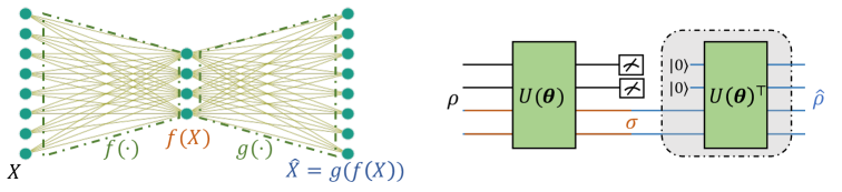
Figure 1: The paradigm of AE and QAE. The left panel illustrates the classical auto-encoder. The right panel shows quantum auto-encoder. In the training process, all quantum operations in the grey box are removed. The state $\sigma$ corresponds to the compressed state of $\rho$. See Section II.2 for explanations.

• We devise the QAE-based fidelity estimator to accomplish low-rank state fidelity estimation problem, which is $\operatorname{\mathsf{DQC}1}$-hard cerezo2020variational . In principle, the runtime complexity of our proposal polynomially scales with the number of qubits, which implies a runtime speedup compared with classical methods. In addition, we prove that the estimation error of our proposal is lower than previous methods. Namely, denote the training error as $\delta$, the estimation error of our proposal scales with $\sqrt{\delta}$, while the estimation error in cerezo2020variational scales with $\delta^{1/4}$. Moreover, we present that our proposal with a slight modification can be constructed by using less quantum resource than previous proposals, i.e., $N$ qubits versus $2N+1$ qubits cerezo2020variational ; chen2020variational . This reduction is crucial in the NISQ era, since the available number of qubits is very limited. Extensive numerical simulations are conducted to support our theoretical results.

• We devise the QAE-based Gibbs state solver to facilitate the quantum Gibbs state preparation task, which has a broad class of applications in quantum simulation, quantum optimization, and quantum machine learning poulin2009sampling . We analyze how the training error of QAE effects the quality of the prepared Gibbs state. Furthermore, we demonstrate the superiority of our scheme than previous methods in the measure of the precision. Numerical simulation results confirm the effectiveness of our proposal.

• We devise the QAE-based quantum Fisher information estimator to determine the best possible estimation error for a certain quantum state. To our best knowledge, this is the first study of applying QAE to address quantum metrology tasks. Compared with prior studies, we prove that our proposal promises a lower estimation error.

The organization of this paper is as follows. In Section II, we recap the mechanism of classical auto-encoder (AE) and quantum auto-encoder (QAE). Then, we analyze the spectral property of QAE in Section III. By leveraging the obtained spectral property, we propose three QAE-based learning protocols, i.e., QAE-based fidelity estimator, QAE-based variational quantum Gibbs state solver, and QAE-based quantum Fisher information estimator in Sections IV, V, and VI, respectively. Last, in Section VII, we conclude this study and discuss future research directions.

II Background

In this section, we first review the mechanism of classical auto-encoder in Subsection II.1 and then introduce the quantum auto-encoder in Subsection II.2.

II.1 Classical auto-encoder

Auto-encoder (AE) is a nearly lossless-compression technique in the context of machine learning and has been broadly applied to information retrieval salakhutdinov2009semantic , anomaly detection zhou2017anomaly , and image processing vincent2008extracting . Intuitively, AE completes the data compression by mapping the given input from a high-dimensional space to a low-dimensional space in the sense that the input can be recovered from this dimension-reduced point. As shown in Figure 1, two basic elements of AE are the encoder $f(\cdot)$ and the decoder $g(\cdot)$, which are realized by neural networks goodfellow2016deep . Suppose that the given dataset is $X\in\mathbb{R}^{m\times n}$ whose $i$-th column $\bm{x}_{i}\in\mathbb{R}^{m}$ represents the $i$-th data point. The encoder $f:\mathbb{R}^{m}\rightarrow\mathbb{R}^{k}$ with $k\ll m$ compresses each data point into a $k$-dimensional space $f(\bm{x}_{i})$, while the decoder $g:\mathbb{R}^{k}\rightarrow\mathbb{R}^{m}$ maps the latent representation $f(\bm{x}_{i})$ to the reconstructed data $\hat{\bm{x}}_{i}=g(f(\bm{x}_{i}))$ goodfellow2016deep . The optimization of AE amounts to minimizing the reconstruction error between the dataset $X$ and its reconstruction $\hat{X}$ whose $i$-th column is $\hat{\bm{x}}_{i}$.

II.2 Quantum auto-encoder

Quantum auto-encoder (QAE), as the quantum analog of AE, is composed of the quantum encoder and the quantum decoder as exhibited in the right panel of Figure 1. The construction of the quantum encoder (or decoder) is completed by variational quantum circuits benedetti2019parameterized ; cerezo2020variational ; du2018expressive ; mitarai2018quantum , which is also called quantum neural networks beer2020training ; farhi2018classification . Mathematically, define an $N$-qubit input state as $\rho\in\mathbb{C}^{2^{N}\times 2^{N}}$ and the number of qubits that represents the latent space as $K$ with $K<N$. Let the quantum encoder be a trainable unitary $U(\bm{\theta})$, where $U(\bm{\theta})=\prod_{l=1}^{L}U_{l}(\bm{\theta})$ and $U_{l}(\bm{\theta})$ is a sequence of parameterized single qubit and two qubits gates with $\bm{\theta}$ being tunable parameters. Under the above setting, QAE aims to find optimal parameters $\bm{\theta}^{*}$ that minimize the loss function $\mathcal{L}(\bm{\theta},\rho)$, i.e.,

$$\mathcal{L}(U(\bm{\theta}),\rho)=\operatorname{Tr}\left(M_{G}U(\bm{\theta})\rho U(\bm{\theta})^{\dagger}\right),$$ (1)

where $M_{G}=\left(\mathbb{I}_{N}-(\ket{0}\bra{0})^{\otimes(N-K)}\otimes\mathbb{I}_{K}\right)$ refers to the measurement operator and $\mathbb{I}_{N}\in\mathbb{R}^{2^{N}\times 2^{N}}$ is the identity.

III Spectral properties of QAE

We now revisit QAE from its spectral properties. Denote the rank of the input state $\rho$ as $r^{*}$ and its spectral decomposition as

$$\rho=\sum_{i=1}^{r^{*}}\lambda_{i}\ket{\psi_{i}}\bra{\psi_{i}}~{}\text{with}~{}\sum_{i=1}^{r^{*}}\lambda_{i}=1,$$ (2)

where $\lambda_{i}$ and $\ket{\psi_{i}}$ are the $i$-th eigenvalues and eigenvectors. Without loss of generality, we suppose $\lambda_{1}\geq\lambda_{2}\geq...\geq\lambda_{r^{*}}$. The optimal $U(\bm{\theta}^{*})$ in Eqn. (1) is shown in the following theorem whose the proof is given in Appendix A.

Theorem 1.

QAE with the loss function $\mathcal{L}(U(\bm{\theta}),\rho)$ in Eqn. (1) has multiple critical (global minimum) points of $U(\bm{\theta}^{*})$. Let $r^{*}=2^{K}$. The generic form of $U(\bm{\theta}^{*})$ is

$$U(\bm{\theta}^{*}):=\sum_{i=1}^{r^{*}}\ket{0}^{\otimes N-K}\ket{\varpi_{i}}\bra{\varphi_{j}}+\sum_{j=r^{*}+1}^{2^{N}}\ket{\phi_{j}}\bra{\varphi_{j}},$$ (3)

where $\{\ket{\phi_{j}}\}_{j=r^{*}+1}\cup\{\ket{0}^{\otimes N-K}\ket{\varpi_{i}}\}_{i=1}^{r^{*}}$ and $\{\ket{\varphi_{j}}\}_{j=1}^{2^{N}}$ are two sets of orthonormal vectors and $\{\ket{\psi}_{i}\}_{i=1}^{r^{*}}$ in Eqn. (2) can be linearly spanned by $\{\ket{\varphi_{j}}\}_{j=1}^{r^{*}}$.

Given access to the optimal quantum encoder $U(\bm{\theta}^{*})$ in Eqn. (3), the compressed state of QAE yields

$$\sigma^{*}=\operatorname{Tr}_{E}\left(\frac{M_{G}U(\bm{\theta}^{*})\rho U(\bm{\theta}^{*})^{\dagger}M_{G}^{\dagger}}{\operatorname{Tr}(M_{G}U(\bm{\theta}^{*})\rho U(\bm{\theta}^{*})^{\dagger})}\right),$$ (4)

where the term ‘$\operatorname{Tr}_{E}(\cdot)$’ represents the partial trace of all qubits except for the $K$ latent qubits nielsen2010quantum . The spectral information between $\sigma^{*}$ and $\rho$ is closely related, as indicated by the following lemma, where the corresponding proof is provided in provided in Appendix B.

Lemma 1.

The compressed state has the same eigenvalues with $\rho$, i.e., $\sigma^{*}=\sum_{i=1}^{r^{*}}\lambda_{i}\ket{\varpi_{i}}\bra{\varpi_{i}}$. Moreover, the subspace spanned by the eigenvectors $\{\ket{\psi_{i}}\}_{i=1}^{r^{*}}$ of $\rho$ can be recovered by $U(\bm{\theta}^{*})$ and eigenvectors $\{\ket{\varpi}_{i}\}_{i=1}^{r^{*}}$.

The result of Lemma 1 indicates that when the input state $\rho$ is low-rank, the spectral information of $\sigma^{*}$ can be efficiently obtained by quantum tomography associated with classical post-processing. In particular, the size of the $K$-qubit compressed state $\sigma^{*}$ scales with $r^{*}\times r^{*}$, which implies that the classical information of $\sigma^{*}$ can be obtained in $O(poly(r^{*}))$ runtime. Moreover, once the classical form of $\sigma^{*}$ is at hand, its spectral decomposition, i.e., $\{\lambda_{i}\}$ and $\{\ket{\varpi_{i}}\}$, can be computed in $O(poly(r^{*}))$ runtime. To this end, the spectral information of $\rho$ can be efficiently acquired via QAE in the optimal case.

In the subsequent sections, we elucidate how to employ QAE, especially the acquired spectral information, to facilitate the low-rank state fidelity estimation, Gibbs state preparation, and quantum metrology tasks. For clarity, here unify some notation about QAE throughout the rest study. Denote the spectral decomposition of the variational quantum circuits $U(\hat{\bm{\theta}})$ as

$$U(\hat{\bm{\theta}}):=\sum_{i=1}^{r}\ket{0}^{\otimes N-K}\ket{\hat{\varpi}_{i}}\bra{\hat{\varphi}_{i}}+\sum_{j=r+1}^{2^{N}}\ket{\hat{\phi}_{j}}\bra{\hat{\varphi}_{j}},$$ (5)

where $\hat{\bm{\theta}}$ refers to the trainable parameters, and $\{\ket{0}^{\otimes N-K}\ket{\hat{\varpi}_{i}}\}_{i=1}^{r}\bigcup\{\ket{\hat{\phi}_{j}}\}_{j=r+1}^{2^{N}}$ and $\{\ket{\hat{\varphi}_{i}}\}_{i=1}^{2^{N}}$ are two sets of orthonormal vectors with $r=2^{K}$. Note that $r$ may not be equal to $r^{*}$ when the training procedure is not optimal. Based on Eqn. (5), the explicit form of the compressed state of QAE in the non-optimal case is

$$\operatorname{\hat{\sigma}}=\operatorname{Tr}_{E}\left(\frac{M_{G}U(\hat{\bm{\theta}})\rho U(\hat{\bm{\theta}})^{\dagger}M_{G}^{\dagger}}{\operatorname{Tr}(M_{G}U(\hat{\bm{\theta}})\rho U(\hat{\bm{\theta}})^{\dagger})}\right)=\sum_{i=1}^{r}\hat{\lambda}_{i}\ket{\hat{\varpi}_{i}}\bra{\hat{\varpi}_{i}},$$ (6)

where $\hat{\lambda}_{i}={\braket{\hat{\varphi}_{i}}{\rho}{\hat{\varphi}_{i}}}/\left({\sum_{j=1}^{r}\braket{\hat{\varphi}_{j}}{\rho}{\hat{\varphi}_{j}}}\right)$.

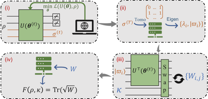
Figure 2: The paradigm of the QAE-based fidelity estimator. The implementation of the QAE-based fidelity estimator is composed of four steps. (i) QAE in Eqn. (1) is applied to optimize $\bm{\theta}$ with $T$ iterations. (ii) After optimization, the compressed state $\sigma^{(T)}$ in Eqn. (10) is extracted into the classical register via quantum state tomography. Once the classical form of $\sigma^{(T)}$ is accessible, the classical Eigen-solver is employed to acquire its spectral information, i.e., $\{\lambda_{i},\ket{\varpi_{i}}\}$. (iii) When the spectral information of $\rho$ is available and the state $\kappa$ is accessible, we can calculate $W$ in Eqn. (8) based on Ref. cerezo2020variational . (iv) Given access to $W$, the fidelity $F(\rho,\kappa)$ can be effectively obtained.

IV QAE-based fidelity estimator

The quantification of the quantum state fidelity plays a central role in verifying and characterizing the states prepared by a quantum processor nielsen2010quantum . In addition, the fidelity measure has also been exploited to study quantum phase transitions gu2010fidelity . Mathematically, the fidelity of two states $\rho$ and $\kappa$ yields

$$F(\rho,\kappa)=\operatorname{Tr}\left(\sqrt{\sqrt{\rho}\kappa\sqrt{\rho}}\right)=\|\sqrt{\rho}\sqrt{\kappa}\|_{1}.$$ (7)

Despite its importance, the calculation of the quantum state fidelity is computationally hard for both classical and quantum devices cerezo2020variational . However, when we slightly relax the problem and target to the low-rank state fidelity estimation (i.e., $\rho$ is low-rank), the following lemma shows that quantum chips may achieve provable advantages over classical devices.

Lemma 2 (Proposition 5, cerezo2020variational ).

The problem of the $N$-qubit low-rank state fidelity estimation within the precision $\pm 1/\text{poly(N)}$ is $\operatorname{\mathsf{DQC}1}$-hard.

Recall that classical computers can not efficiently simulate $\operatorname{\mathsf{DQC}1}$ models unless the polynomial-time hierarchy collapses to the second level fujii2018impossibility . The result of Lemma 2 shows that if a quantum algorithm can accomplish the low-rank state fidelity estimation in polynomial runtime, then this algorithm possesses a provable runtime advantage compared with the optimal classical method.

Here we devise a QAE-based fidelity estimator, which has the ability to complete the the low-rank state fidelity estimation task in a polynomial runtime. The underlying concept of our proposal is as follows. Note that

$$\operatorname{F}(\rho,\kappa)=\operatorname{Tr}\left(\left(\sum_{i,j}W_{i,j}\ket{\psi_{i}}\bra{\psi_{j}}\right)^{-1/2}\right),$$ (8)

where $W_{i,j}=\sqrt{\lambda_{i}\lambda_{j}}\braket{\psi_{i}}{\kappa}{\psi_{j}}$ for $\forall i\in[r^{*}]$. In other words, the calculation of $\operatorname{F}(\rho,\kappa)$ amounts to acquiring $W\in\mathbb{C}^{r^{*}\times r^{*}}$, which can be effectively achieved once the state $\kappa$ and the eigenvalues and eigenvectors of $\rho$ are accessible. The spectral information of $\rho$ provided by QAE allows us to efficiently estimate the fidelity $\operatorname{F}(\rho,\kappa)$ defined in Eqn. (7) in $O(poly(N))$ runtime.

In the following two subsections, we first present the implementation details of our proposal, followed by the numerical simulations.

IV.1 Implementation of QAE-based fidelity estimator

We now elaborate on the protocol of the QAE-based fidelity estimator. As shown in Figure 2, the proposed method consists of four steps.

1. We apply QAE formulated in Eqn. (1) to compress the given state $\rho$. Let the total number of training iterations be $T$. The updating rule of the parameters $\bm{\theta}$ at the $t$-th iteration yields

   $$\bm{\theta}^{(t+1)}=\bm{\theta}^{(t)}+\eta\frac{\partial\mathcal{L}(U(\bm{\theta^{(t)}}),\rho)}{\partial\bm{\theta}^{(t)}},$$ (9)

   where $\eta$ refers to the learning rate. The gradients $\partial\mathcal{L}(U(\bm{\theta^{(t)}}),\rho)/\partial\bm{\theta}^{(t)}$ can be acquired by using the parameter shift rule mitarai2018quantum ; schuld2019evaluating . After the optimization is completed, the trained parameters $\bm{\theta}^{(T)}$ are exploited to prepare the compressed state in Eqn. (6),

   $$\sigma^{(T)}=\operatorname{Tr}_{E}\left(\frac{M_{G}U(\bm{\theta}^{(T)})\rho U(\bm{\theta}^{(T)})^{\dagger}M_{G}^{\dagger}}{\operatorname{Tr}(M_{G}U(\bm{\theta}^{(T)})\rho U(\bm{\theta}^{(T)})^{\dagger})}\right).$$ (10)

2. The quantum state tomography techniques nielsen2010quantum are applied to $\sigma^{(T)}$ with size $2^{K}\times 2^{K}$ to obtain the classical information of the compressed state. Note that for simplicity, here we only focus on the ideal case with the infinite number of measurements so that the state $\sigma^{(T)}$ can be exactly recorded in the classical register. When the measurement error is considered, the likelihood recovering strategy can be used to efficiently find the closest probability distribution of $\sigma^{(T)}$ smolin2012efficient . Once the classical form of $\sigma^{(T)}$ is in hand, its spectral information can be effectively obtained when the number of latent qubits $K$ is small. With a slight abuse of notation, the eigenvalues and eigenvectors of $\sigma^{(T)}$ are denoted by $\{\hat{\lambda}_{i}\}_{i=1}^{r}$ and $\{\hat{\varpi}_{i}\}_{i=1}^{r}$ with $r=2^{K}$, respectively, i.e.,

   $$\sigma^{(T)}=\sum_{i=1}^{r}\hat{\lambda}_{i}\ket{\hat{\varpi}_{i}}\bra{\hat{\varpi}_{i}}.$$ (11)

   We remark that given access to $\{\ket{\hat{\varpi}_{i}}\}$ and $U(\hat{\bm{\theta}})$, we can prepare quantum states $\{\ket{\hat{\varphi}_{i}}\}$, i.e.,

   $$\ket{\hat{\varphi}_{i}}=U(\bm{\theta}^{(T)})^{\dagger}\ket{0}^{\otimes(N-k)}\ket{\hat{\varpi}_{i}},$$ (12)

   which occupy the same subspace spanned by the eigenvectors of $\rho$.

3. The classical spectral information of $\sigma^{(T)}$, the variational quantum circuits $U(\bm{\theta}^{(T)})^{\dagger}$, and the state $\kappa$, are employed to estimate $W_{ij}$ in Eqn. (8). The element $W_{ij}$ is approximated by

   $$\widehat{W}_{ij}=\sqrt{\hat{\lambda}_{i}\hat{\lambda}_{j}}\langle\hat{\varphi}_{i}|\kappa|\hat{\varphi}_{j}\rangle,~{}\forall i,j\in[r].$$ (13)

   A possible physical implementation to achieve $\langle\hat{\varphi}_{i}|\kappa|\hat{\varphi}_{j}\rangle$ in $\widehat{W}_{ij}$ is using the destructive Swap test circuit subacsi2019entanglement , which is identical to cerezo2020variational .

4. The fidelity $F(\rho,\kappa)$ is approximated via the classical post-processing. In particular, given access to the matrix $\widehat{W}$ with size $2^{K}\times 2^{K}$, we use $\operatorname{\widehat{F}}(\rho,\kappa)=\operatorname{Tr}(\sqrt{\widehat{W}})$ to estimate $F(\rho,\kappa)$.

We remark that seeking the optimal parameter $\bm{\theta}^{*}$ of QAE is challenging during a finite number of iterations. Let the trained parameters of QAE after $T$ iterations be $\hat{\bm{\theta}}$ and the loss be $\mathcal{L}(U(\hat{\bm{\theta}}),\rho)=\delta$. Denote $r=2^{K}$ and the compressed state of $\rho$ as $\operatorname{\hat{\sigma}}\in\mathbb{C}^{r\times r}$ and its spectral decomposition as $\{\hat{\lambda}_{i}\}$ and $\{\ket{\hat{\varpi}_{i}}\}$. Given the spectral information of $\operatorname{\hat{\sigma}}$, the fidelity $\operatorname{F}(\rho,\kappa)$ is estimated by

$$\operatorname{\widehat{F}}(\rho,\kappa)=\operatorname{Tr}((\sum_{i,j}\sqrt{\hat{\lambda}_{i}\hat{\lambda}_{j}}\braket{\hat{\varphi}_{i}}{\kappa}{\hat{\varphi}_{i}}\ket{\hat{\varphi}_{i}}\bra{\hat{\varphi}_{j}})^{-1/2}),$$ (14)

where $\ket{\hat{\varphi}_{i}}=U(\hat{\bm{\theta}})\ket{0^{\otimes N-K},\varpi_{i}}$. The following theorem indicates that the discrepancy between $\operatorname{F}(\rho,\kappa)$ and $\operatorname{\widehat{F}}(\rho,\kappa)$ is bounded by the loss $\delta$.

Theorem 2.

Suppose that the training loss of QAE in Eqn. (1) yields $\mathcal{L}(U(\bm{\theta}^{(T)}),\rho)=\delta$. The QAE-based fidelity estimator returns $\operatorname{\widehat{F}}(\rho,\kappa)$ in Eqn. (14) with

$$\operatorname{\widehat{F}}(\rho,\kappa)-\sqrt{2\delta}\leq\operatorname{F}(\rho,\kappa)\leq\operatorname{\widehat{F}}(\rho,\kappa)+\sqrt{2\delta}.$$ (15)

The proof of Theorem 2 is provided in Appendix C. The achieved results affirm that the estimated fidelity $\operatorname{\widehat{F}}(\rho,\kappa)$ can be used to infer $\operatorname{F}(\rho,\kappa)$, even though the optimization of QAE is not optimal. Furthermore, when $\delta$ is large, the bound in Eqn. (15) will be very loose and impractical. In other words, it is necessary to adopt advanced optimization techniques cerezo2020cost ; du2020quantumQAS ; zhang2020toward to improve the trainability of QAE to suppress the error term $\delta$. Notably, the estimator error achieved by QAE is lower than the error bound obtained by the fidelity estimator cerezo2020variational , since their error bound depends on $\delta^{1/4}$ and the rank $r^{*}$ (See Appendix D). The improved error bound is important to gain quantum advantages, supported by Lemma 2.

IV.2 Numerical simulations

We conduct numerical simulations to evaluate performance of QAE for the fidelity estimation of low-rank states. In particular, we set $\rho$ and $\kappa$ as two eight-qubit states (i.e., $N=8$) with rank $r^{*}=8$ and $r^{*}=17$, respectively. Both $\rho$ and $\kappa$ are prepared by a pure state followed by a tunable noisy channel $\mathcal{N}(\cdot)$. In simulations, we vary the size of latent space by setting $K=1,...,7$. To benchmark performance of QAE, we also apply sub-fidelity and super-fidelity bounds (SSFB) to estimate $\operatorname{F}(\rho,\kappa)$ miszczak2009sub . The hyper-parameters setting is as follows. The number of iterations is set as $200$. The hardware-efficient ansatz benedetti2019parameterized is employed to implement the quantum encoder $U(\bm{\theta})=\prod_{l=1}^{L}U_{l}(\bm{\theta})$ with $L=5$. See Appendix D for construction details.

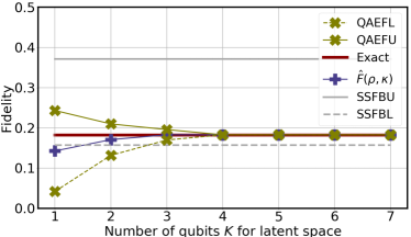
Figure 3: The simulation results of the fidelity estimation. The labels QAEFL and QAEFU refer to $\operatorname{\widehat{F}}(\rho,\kappa)-\sqrt{2\delta}$ and $\operatorname{\widehat{F}}(\rho,\kappa)+\sqrt{2\delta}$ in Theorem 2, respectively, where $\delta$ is the loss of QAE. The label ‘SSFBU’ (‘SSFBL’) is super-fidelity (sub-fidelity) bounds in miszczak2009sub .

The simulation results are exhibited in Figure 3. The blue solid line refers to the estimated fidelity $\operatorname{\widehat{F}}(\rho,\kappa)$ achieved by the QAE-based fidelity estimator, which fast converges to the true fidelity $\operatorname{F}(\rho,\kappa)$ highlighted by the red solid line with respect to the increased $K$. Note that, even though the training loss of QAE is considered, the estimated bounds $\operatorname{\widehat{F}}(\rho,\kappa)\pm\sqrt{2\delta}$ also fast converge to the true fidelity $\operatorname{F}(\rho,\kappa)$, as indicated by the green solid and dashed line with cross markers. Such an observation accords with Theorem 2. Moreover, our proposal achieves better performance than SSFB methods (the solid and dashed grey lines) when $K\geq 3$. This result suggests the superiority of QAE when the number of latent qubits satisfies $2^{K}\geq r^{*}$. See Appendix D for more simulation results and discussions.

We remark that with a slight modification, it is sufficient to use $N$ qubits to realize the QAE-based fidelity estimator for estimating the fidelity of two $N$-qubit states (See Appendix E), while previous proposals require at least $2N+1$ qubits cerezo2020variational ; chen2020variational . This implies that the modified QAE-based fidelity estimator is resource-efficient, which is crucial for NISQ machines with limited number of qubits.

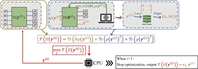
Figure 4: The paradigm of the QAE-based variational quantum Gibbs state solver. The implementation of the QAE-based variational quantum Gibbs state solver is composed of three components. The first component is the variational quantum circuit $U(\bm{\gamma}^{(t)})$ to prepare the variational quantum Gibbs state $\rho(\bm{\gamma}^{(t)})$. The second component is QAE, which is used to extract the spectral information of $\rho(\bm{\gamma}^{(t)})$. The third component is the classical processor to optimize the variational quantum circuit $U(\bm{\gamma}^{(t)})$ and the quantum encoder $U(\bm{\theta}^{(t)})$. The learning procedure at each step is as follows. (i) The variational quantum circuit $U(\bm{\gamma}^{(t)})$ is employed to compute $\operatorname{Tr}(H\rho(\bm{\gamma}^{(t)}))$. (ii) QAE is leveraged to compress the state $\rho(\bm{\gamma}^{(t)})$ prepared by $U(\bm{\gamma}^{(t)})$ into the state $\sigma^{(t)}$. (iii) Applying the quantum tomography and the classical decomposition on $\sigma^{(t)}$ gives $\{\operatorname{Tr}(\rho(\bm{\gamma})^{j+1})\}$ required in Eqn. (19). The collected results $\operatorname{Tr}(H\rho(\bm{\gamma}^{(t)}))$ and $\{\operatorname{Tr}(\rho(\bm{\gamma})^{j+1})\}$ form the $R$-truncated free energy $\mathcal{F}_{R}(\rho(\bm{\gamma}^{(t)}))$ and allows the updating of $\gamma^{(t)}$. Repeating the above procedures with $T$ times, the classical processor outputs $\gamma^{(T)}$, which can be used to prepared the estimated Gibbs state $\rho(\bm{\gamma}^{(T)})$.

V QAE-based variational quantum Gibbs state solver

The preparation of quantum Gibbs states is a central problem in quantum simulation, quantum optimization, and quantum machine learning poulin2009sampling . For example, the quantum semi-definite programs exploit quantum Gibbs states to earn runtime speedups brandao2017quantum . Mathematically, the explicit form of quantum Gibbs states, which describe the thermal equilibrium properties of quantum systems, is

$$\rho_{G}=\frac{e^{-\beta H}}{\operatorname{Tr}(e^{-\beta H})},$$ (16)

where $\beta$ refers to the inverse temperature and $H\in\mathbb{C}^{2^{N}\times 2^{N}}$ is a specified Hamiltonian. However, theoretical results based on computational complexity theory Watrous2009 indicate that the preparation of quantum Gibbs states at low-temperature is difficult, i.e., computing the partition function $\operatorname{Tr}(e^{-\beta H})$ in two-dimensions is $\operatorname{\mathsf{NP}}$-hard schuch2007computational . Driven by the significance and the intrinsic hardness of preparation, Ref. wang2020variational explored how to use variational quantum circuits implemented on NISQ devices to generate a state $\rho(\bm{\gamma}^{*})\in\mathbb{C}^{2^{N}\times 2^{N}}$ approximating $\rho_{G}$. In particular, the state $\rho(\bm{\gamma}^{*})$ minimizes the free energy $\mathcal{F}$ such that

$$\rho(\bm{\gamma}^{*})=\arg\min_{\rho(\bm{\gamma})}\mathcal{F}(\rho(\bm{\gamma})),$$ (17)

where $\mathcal{F}(\rho(\bm{\gamma}))=\operatorname{Tr}(H\rho(\bm{\gamma}))-\beta^{-1}S(\rho(\bm{\gamma}))$ and $S(\rho(\bm{\gamma}))$ refers to the von Neumann entropy nielsen2010quantum . To further improve the computational efficiency, the proposal wang2020variational replaces $S(\rho(\bm{\gamma}))$ with its truncated version, i.e., $S_{R}(\rho(\bm{\gamma}))=\sum_{j=0}^{R}C_{j}\operatorname{Tr}(\rho(\bm{\gamma})^{j+1})$ with $C_{j}$ being certain constants. When $S(\rho(\bm{\gamma}))$ is estimated by $S_{2}(\rho(\bm{\gamma}))$, the loss function $\mathcal{F}(\rho(\bm{\gamma}))$ used to optimize the state $\rho(\bm{\gamma})$ yields

$$\arg\min_{\rho(\bm{\gamma})}\operatorname{Tr}(H\rho(\bm{\gamma}))-\frac{2\operatorname{Tr}(\rho(\bm{\gamma})^{2})}{\beta}-\frac{\operatorname{Tr}(\rho(\bm{\gamma})^{3})+3}{2\beta}.$$ (18)

The calculation of the terms $\operatorname{Tr}(\rho(\bm{\gamma})^{2})$ and $\operatorname{Tr}(\rho(\bm{\gamma})^{3})$ is completed by using the destructive Swap test subacsi2019entanglement . Nevertheless, this method is resource-inefficient (see Appendix F for explanations), where the required number of qubits is linearly scaled by a factor of two and three over the calculation of $\operatorname{Tr}(H\rho(\bm{\gamma}))$, respectively.

Enlightened by the fact that the two terms $\operatorname{Tr}(\rho(\bm{\gamma})^{2})$ and $\operatorname{Tr}(\rho(\bm{\gamma})^{3})$ can be effectively obtained by using the eigenvalues of $\rho(\bm{\gamma})$, here we apply QAE to calculate these two terms. In this way, the required quantum resource can be dramatically reduced compared with the destructive Swap test strategy. Specifically, in the optimal case, the spectral information acquired by the compressed state $\sigma^{*}$, i.e., a set of eigenvalues $\{\lambda_{i}\}_{i=1}^{r^{*}}$, is sufficient to recover the oriented two terms, where $\operatorname{Tr}(\rho(\bm{\gamma})^{2})=\sum_{i}\lambda_{i}^{2}$ and $\operatorname{Tr}(\rho(\bm{\gamma})^{3})=\sum_{i}\lambda_{i}^{3}$.

We now elaborate on the implementation details of the proposed QAE-based variational quantum Gibbs state solver as shown in Figure 4. Suppose that the total number of iterations to optimize the $R$-truncated free energy $\mathcal{F}_{R}(\rho(\bm{\gamma}^{(t)}))$ is $T_{1}$. The mechanism of our proposal at the $t$-th iteration with $t\in[T_{1}]$ is as follows.

1. The variational quantum Gibbs state $\rho(\bm{\gamma}^{(t)})$ prepared by the variational quantum circuit $U(\bm{\gamma}^{(t)}))$, i.e., $\rho(\bm{\gamma}^{(t)})=U(\bm{\gamma}^{(t)}))(\ket{\bm{0}}\bra{\bm{0}})U(\bm{\gamma}^{(t)}))^{\dagger}$, is interacted with $H$ to compute $\operatorname{Tr}(H\rho(\bm{\gamma}^{(t)}))$, as highlighted by the brown box in Figure 4.

2. QAE is employed to compress the state $\rho(\bm{\gamma}^{(t)})$ prepared by $U(\bm{\gamma}^{(t)}))$. Once the optimization of QAE is completed, the compressed state $\sigma^{(T)}$ is extracted into the classical form followed by the spectral decomposition $\{\lambda_{i}\}$. This step is highlighted by the blue box in Figure 4.

3. Since the trace term $\operatorname{Tr}(\rho(\bm{\gamma})^{j+1})$ equals to $\sum_{i}\lambda_{i}^{j+1}$, the terms $\{\operatorname{Tr}(\rho(\bm{\gamma})^{j+1})\}_{j=1}^{R}$ can be efficiently evaluated. Through feeding the collected $\{\operatorname{Tr}(\rho(\bm{\gamma})^{j+1})\}$ and $\operatorname{Tr}(H\rho(\bm{\gamma}^{(t)}))$ into the classical computer, the $R$-truncated free energy $\mathcal{F}_{R}(\rho(\bm{\gamma}^{(t)}))$ can be inferred following Eqn. (17). The mechanism of calculating $\mathcal{F}_{R}(\rho(\bm{\gamma}^{(t)}))$ allows the QAE-based variational quantum Gibbs state solver to utilize the parameter shift rule to update the trainable parameters $\bm{\gamma}$ to complete the $t$-th iteration, i.e.,

   $$\bm{\gamma}^{(t+1)}=\bm{\gamma}^{(t)}+\eta\frac{\partial\mathcal{F}_{R}(\rho(\bm{\gamma}^{(t)}))}{\partial\bm{\gamma}^{(t)}}.$$ (19)

After repeating the above procedures with in total $T_{1}$ iterations, the QAE-based variational quantum Gibbs state solver outputs $\epsilon_{1}=\mathcal{F}_{R}(\rho(\bm{\gamma}^{(T)}))$ and the trained parameters $\bm{\gamma}^{(T)}$.

We emphasize that the key difference between our proposal and the method in wang2020variational is the way to acquire $\{\operatorname{Tr}(\rho(\bm{\gamma})^{j+1})\}$. This difference leads to the following lemma, which quantifies the lower bound of the fidelity between the target state $\rho_{G}$ and the state $\rho(\hat{\bm{\gamma}})$ prepared by the QAE-based variational quantum Gibbs state solver. The corresponding proof is provided in Appendix G.

Lemma 3.

Following notation in Eqn. (17), let $\hat{\bm{\gamma}}$ be the optimized parameters of the QAE-based variational quantum Gibbs state solver and $r$ be the rank of $\rho(\hat{\bm{\gamma}})$. Denote $\epsilon_{1}$ as the tolerable error. When QAE in Eqn. (1) is used to acquire eigenvalues of $\rho(\hat{\bm{\gamma}})$ with training loss $\delta$, the fidelity between the approximated state $\rho(\hat{\bm{\gamma}})$ and the oriented state $\rho_{G}$ is lower bounded by

$$\operatorname{F}(\rho_{G},\rho(\hat{\bm{\gamma}}))\geq 1-\sqrt{2\beta\epsilon+\frac{C_{\max}\delta}{1-\delta}},$$ (20)

where $\epsilon=\epsilon_{1}+\frac{2r}{R+1}(1-\Delta)^{R+1}$ and $\Delta\in(0,e^{-1})$ is a constant determined by the truncation number $R$.

The achieved results demonstrate that even though the optimization of QAE is not optimal, the collected spectral information of the compressed state can also be used to quantify the trace terms, while the price to pay is slightly decreasing the fidelity between $\rho(\bm{\gamma})$ and $\rho_{G}$. Furthermore, when the inverse temperature $\beta$, rank $r$, and the training loss of QAE $\delta$ are small, the prepared state $\rho(\bm{\gamma})$ can well approximate the target state $\rho_{G}$ in Eqn. (16). This observation suggests to exploit advanced optimization techniques du2020learnability ; zhang2020toward ; du2020quantumQAS ; cerezo2020cost to improve the trainability of QAE and hence the performance of the QAE-based variational quantum Gibbs state solver.

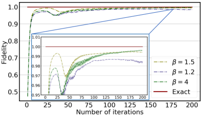
Figure 5: The fidelity $\operatorname{F}(\rho(\bm{\gamma}),\rho_{G})$ with varied $\beta$. The label ‘$\beta=x$’ represents how the fidelity $\operatorname{F}(\rho(\bm{\gamma}),\rho_{G})$ evolves in $T=200$ iterations when $\beta$ in Eqn. (16) is set as $x$.

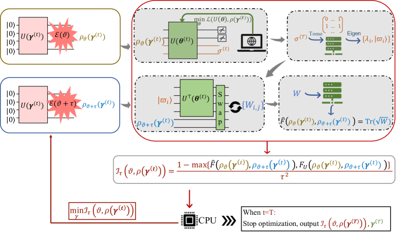
Figure 6: The paradigm of the QAE-based QFI estimator. The QAE-based QFI estimator is implemented on a quantum-classical hybrid system. In the quantum part, a variational quantum circuit $U(\bm{\gamma})$ is employed to prepare the tunable probe state $\rho(\bm{\gamma})$. This probe state is separated interacted with the source described by the parameter $\vartheta$ and $\vartheta+\tau$ to prepare the state $\rho_{\vartheta}(\bm{\gamma})$ and $\rho_{\vartheta+\tau}(\bm{\gamma})$. The two generated states are fed into the QAE-based fidelity estimator to estimate $\operatorname{F}(\rho_{\vartheta}(\bm{\gamma}),\rho_{\vartheta+\tau}(\bm{\gamma}))$, as highlighted by the red box. The calculated fidelity is used to compute $\mathcal{I}_{\tau}(\vartheta,\rho_{\vartheta}(\bm{\gamma}))$ in Eqn. (21) and then update parameters $\bm{\gamma}$ to maximize this quantity. Repeating the above procedures with $T$ times, the classical processor outputs $\gamma^{(T)}$, which can be used to prepared the estimated Gibbs state $\rho(\bm{\gamma}^{(T)})$.

V.1 Numerical simulations

We apply our proposal to prepare the Gibbs state $\rho_{G}$ corresponding to the Ising chain model, where the Hamiltonian in Eqn. (16) is $H_{B}=-\sum_{i=1}^{J}Z_{i}Z_{i+1}$, $Z_{J+1}=Z_{1}$, and $Z_{i}$ is the Pauli-Z matrix on the $i$-th qubit. We set $J=3$ and $\beta=\{1.2,1.5,4\}$. The hyper-parameters setting is as follows. The total number of iterations to optimize $\mathcal{F}(\rho(\bm{\gamma}))$ in Eqn. (18) is set as $T=200$. At the $t$-th iteration, QAE is employed to estimate the eigenvalues of $\rho(\bm{\gamma}^{(t)})$ to compute the last two terms in Eqn. (18). The number of inner loops to optimize the quantum encoder $U(\bm{\theta})$ is set as $100$. Refer to Appendix F for more simulation details.

The simulation results are illustrated in Figure 5. For all settings $\beta=\{1.2,1.5,4\}$, the fidelity between the prepared quantum Gibbs state $\rho(\bm{\gamma})$ and the target state $\rho_{G}$ is above $98\%$ after $100$ iterations. In particular, the fidelity $\operatorname{F}(\rho(\bm{\gamma}),\rho_{G})$ converges to $98.5\%$, $99.5\%$, and $99.6\%$ for the setting $\beta=1.2$, $1.5$, and $4$, respectively. The high fidelity for all settings reflect the feasibility of the proposed QAE-based variational quantum Gibbs state solver. Moreover, the degraded performance with respect to the decreased $\beta$ accords with Lemma 3, i.e., a smaller $\beta$ leads to a worse fidelity bound.

VI QAE-based quantum Fisher information estimator

The high precision of sensing is of great importance to many scientific and real-world applications, which include but not limit to chemical structure identification lovchinsky2016nuclear and gravitational wave detection mcculler2020frequency . However, the central limit theorem indicates that the statistical error in the classical scenario must be lower bounded by $\nu^{-1/2}$, where $\nu$ is the number of measurements. Driven by the significance of improving the precision of sensing, it highly desired to utilize quantum effects to further reduce the statistical error.

Quantum metrology provides a positive response towards the above question giovannetti2006quantum ; giovannetti2011advances ; koczor2020variational . In particular, through leveraging coherence or entangled quantum states, the statistical error can be reduced by an amount proportional to $\nu^{-1}$. A fundamental quantity in quantum metrology is quantum Fisher information (QFI) petz2011introduction , which determines the best possible estimation error for a certain quantum state. Mathematically, let $\rho_{\vartheta}(\bm{\gamma})$ be the exact state, which is prepared by interacting a tunable $N$-qubit state $\rho(\bm{\gamma})$ with a source that encodes the environmental information in a single parameter $\vartheta$. The QFI $\mathcal{I}(\vartheta;\rho_{\vartheta}(\bm{\gamma}))$ measures the ultimate precision $\Delta\vartheta$, i.e., $(\Delta\vartheta)^{2}\geq 1/(\nu\mathcal{I}(\vartheta;\rho_{\vartheta}(\bm{\gamma})))$, where $\nu$ is the number of measurements to estimate $\vartheta$. At the expense of computational simplicity, $\mathcal{I}(\vartheta;\rho_{\vartheta}(\bm{\gamma}))$ is generally estimated by

$$\mathcal{I}_{\tau}(\vartheta;\rho_{\vartheta})=8\frac{1-\operatorname{F}(\rho_{\vartheta},\rho_{\vartheta+\tau})}{\tau^{2}}.$$ (21)

When $\tau\rightarrow 0$, the approximation error degrades to $0$, i.e., $\mathcal{I}_{\delta}(\vartheta;\rho_{\vartheta}(\bm{\gamma}))=\mathcal{I}_{\tau\rightarrow 0}(\vartheta;\rho_{\vartheta}(\bm{\gamma}))$. Intuitively, a true state $\rho_{\vartheta}(\bm{\gamma})$ with a high QFI $\mathcal{I}_{\tau}(\vartheta;\rho_{\vartheta}(\bm{\gamma}))$ is sharply different from the error state $\rho_{\vartheta+\tau}(\bm{\gamma})$, which implies that the parameter $\vartheta$ can be effectively estimated via measurement.

As indicated in Lemma 2, the calculation of the fidelity $\operatorname{F}(\rho_{\vartheta}(\bm{\gamma}),\rho_{\vartheta+\tau}(\bm{\gamma}))$ in Eqn. (21) is computationally hard for general mixed states. Such an inefficiency prohibits the applicability of quantum metrology. To address this issue, the study beckey2020variational generalized the fidelity estimation solver cerezo2020variational to estimate $\mathcal{I}_{\tau}(\vartheta;\rho_{\vartheta}(\bm{\gamma}))$ with potential runtime advantages. Intuitively, their proposal employs variational quantum circuits to prepare states $\rho_{\vartheta}(\bm{\gamma})$ and $\rho_{\vartheta+\tau}(\bm{\gamma})$ by adjusting $\bm{\gamma}$. Once these two quantum states are prepared, the variational fidelity estimator cerezo2020variational is applied to estimate $\mathcal{I}_{\tau}(\vartheta;\rho_{\vartheta}(\bm{\gamma}))$. The optimization is conducted to find optimal $\bm{\gamma}^{*}$ that maximizes $\mathcal{I}_{\tau}(\vartheta;\rho_{\vartheta}(\bm{\gamma}))$.

Here we combine variational quantum circuits with the QAE-based fidelity estimator to construct a more advanced QFI estimator. Recall that to balance the computational efficiency and the learning performance, the variational QFI estimator in beckey2020variational exploits the variational fidelity estimator to estimate $\operatorname{F}(\rho_{\vartheta}(\bm{\gamma}),\rho_{\vartheta+\tau}(\bm{\gamma}))$. Considering that the QAE-based fidelity estimator promises a lower estimation error than that of the variational QFI estimator as proved in Theorem 2, it is natural to substitute the variational QFI estimator with the QAE-based fidelity estimator to devise the QAE-based QFI estimator.

The implementation of the QAE-based QFI estimator is illustrated in Figure 6. In particular, the proposed algorithm repeats the following procedure with in total $T$ times. At the $t$-th iteration, the variational quantum circuit $U(\bm{\gamma}^{(t)})$ is utilized to generate the probe state $\rho(\bm{\gamma}^{(t)})$. As highlighted by the brown and blue box, the probe state separately interacts with the target source described by the parameter $\vartheta$ and $\vartheta+\tau$ to generate the state $\rho_{\vartheta}(\bm{\gamma})$ and $\rho_{\vartheta+\tau}(\bm{\gamma})$. These two states, which contain the information of source, are fed into the QAE-based fidelity estimator as introduced in Section IV. The estimated fidelity returned by the QAE-based fidelity estimator is employed to compute $\mathcal{I}_{\tau}(\vartheta,\rho_{\vartheta}(\bm{\gamma}))$ in Eqn. (21) and then update parameters $\bm{\gamma}$ to maximize this quantity. This completes the $t$-th iteration.

The following lemma quantifies how the training error of QAE influences the performance of the proposed . The proof of the above lemma is provided in Appendix I.

Lemma 4.

Following notations in Eqns. (1) and (21), let $r$ be the rank of $\rho_{\vartheta}(\bm{\gamma})$. When QAE is applied to estimate the fidelity $\operatorname{F}(\rho_{\vartheta}(\bm{\gamma}),\rho_{\vartheta+\tau}(\bm{\gamma}))$ with training loss $\delta$. Then the QAE-based QFI estimator returns $\hat{\mathcal{I}}_{\tau}(\vartheta;\rho_{\vartheta})$ with

$$\left|\hat{\mathcal{I}}_{\tau}(\vartheta,\rho_{\vartheta}(\bm{\gamma}))-\mathcal{I}_{\tau}(\vartheta,\rho_{\vartheta}(\bm{\gamma}))\right|\leq\frac{8\sqrt{2\delta}}{\tau^{2}}.$$ (22)

The above results imply that the estimation error is controlled by the training loss $\delta$. As with prior two QAE-based learning protocols, this dependence requests us to inject error mitigation techniques and advanced optimizers into QAE to improve the performance of the QAE-based QFI estimator. Moreover, celebrated by the advance of the QAE-based fidelity estimator in Theorem 2, our proposal achieves a better error bound than that of beckey2020variational .

VI.1 Numerical simulations

We apply the QAE-based QFI estimator to prepare the probe state $\rho(\bm{\gamma})$ that maximizes the QFI for a magnetic field described by the parameter $\vartheta$. Mathematically, the probe state interacting with the magnetic field transforms to $\rho_{\vartheta}(\bm{\gamma})=W(\vartheta)\rho(\bm{\gamma})W(\vartheta)^{\dagger}$, where $W(\vartheta)=e^{-i\vartheta G}$ is a unitary transformation and $G=\sum_{i=1}^{J}Z_{i}$ is the specified Hamiltonian and $Z_{i}$ is the Panli-Z matrix on the $i$-th qubit. We set $J=3$ and the number of iterations to optimize $\bm{\gamma}$ as $75$. At each iteration, the QAE-based fidelity estimator is exploited to estimate $\operatorname{F}(\rho_{\vartheta}(\bm{\gamma}^{(t)}),\rho_{\vartheta+\tau}(\bm{\gamma}^{(t)}))$, where the number of the latent qubits is $K=2$. The number of inner loops to optimize the quantum encoder $U(\bm{\theta})$ is $100$.

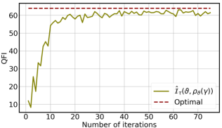
Figure 7: The simulation results of the QAE-based QFI estimator. The label ‘Optimal’ represents the maximum QFI that can be achieved. The label ‘$\hat{\mathcal{I}}_{\tau}(\vartheta,\rho_{\vartheta}(\bm{\gamma}))$’ represents QFI estimated by the QAE-based QFI estimator.

The simulation results are exhibited in Figure 7. Recall that a well-known conclusion in quantum sensing is that the optimal probe state is an $N$-qubit GHZ state in the noiseless scenario, where the QFI reaches the Heisenberg limit $4N^{2}$. Compared with the optimal result, the QFI of the prepared probe state converges to the optimal QFI, i.e., $64$, after $30$ iterations. The achieved results indicate the applicability of the QAE-based QFI estimator.

VII Discussion and conclusion

In this study, we revisit QAE from its spectral properties and demonstrate how to exploit these spectral information to benefit quantum computation, quantum information, and quantum sensing tasks. Compared with the previous literature, the QAE-based methods can achieve better error bounds and can be more resource-efficient. These improved error bounds are crucial to utilize QAE-based methods to achieve quantum advantages. Moreover, we carry out extensive numerical simulations to validate the effectiveness of our proposals. Our work contributes to many tasks in the field of quantum computing, quantum simulation, and quantum information processing, since the developed techniques enable a reduction of the required quantum resource such as the quantum memory and the number of quantum gates.

The achieved theoretical results provide strong evidence that the performance of the proposed QAE-based learning protocols heavily depend on the training loss $\delta$. Hence, for the purpose of attaining good performance, it is vital to investigate what advanced optimizers stokes2020quantum ; wierichs2020avoiding and powerful error mitigation techniques endo2018practical ; li2017efficient ; mcclean2017hybrid ; temme2017error can effectively suppress $\delta$.

A major caveat of variational quantum algorithms is barren plateaus mcclean2018barren , where the gradients information is exponentially vanished in terms of the qubit counts and circuit depth. Different from other algorithms, the study cerezo2020cost has proposed a local measurement based QAE and proved its good trainability. In other words, QAE is a promising solution to avoid barren plateaus. With this regard, it is intrigued to exploit the applicability of such QAE-based methods and analyze its error bounds for various tasks.

In the end, we would like to remark that QAE may also facilitate many other learning problems. A potential candidate is quantum machine learning du2021efficient ; huang2020experimental ; qian2021dilemma ; schuld2019quantum ; wu2021expressivity . Recall that recent studies have exhibited the potential of quantum kernels to earn quantum advantages havlivcek2019supervised ; hubregtsen2021training ; kusumoto2021experimental ; schuld2021supervised ; wang2021towards . Note that the core of quantum kernels is calculating the similarity of two quantum inputs, which amounts to accomplishing the fidelity estimation. In this perspective, a future research direction is to explore whether the QAE-based fidelity estimator can boost the performance of quantum kernels.

Appendix

Appendix A Proof of Theorem 1

Proof of Theorem 1.

Note that the loss $\mathcal{L}$ defined in Eqn. (1) is lower bounded by $0$, i.e.,

$$\mathcal{L}(U(\bm{\theta}),\rho)=\operatorname{Tr}\left(M_{G}U(\bm{\theta})\rho U(\bm{\theta})^{\dagger}\right)=\operatorname{Tr}\left(\left(\mathbb{I}_{N}-(\ket{0}\bra{0})^{\otimes(N-K)}\otimes\mathbb{I}_{K}\right)U(\bm{\theta})\rho U(\bm{\theta})^{\dagger}\right)\geq 0,$$ (23)

since both the measurement operator $M_{G}$ and the state $U(\bm{\theta})\rho U(\bm{\theta})^{\dagger}$ are positive semi-definite matrices. Such a result implies that the optimal parameters $\bm{\theta}^{*}$, or equivalently $U(\bm{\theta}^{*})$, satisfy

$$\mathcal{L}(U(\bm{\theta}^{*}),\rho)=0.$$ (24)

We next derive the explicit form of $U(\bm{\theta}^{*})$ that enables $\mathcal{L}(U(\bm{\theta}^{*}),\rho)=0$. Recall that the loss function $\mathcal{L}(U(\bm{\theta}),\rho)$ can be rewritten as

$$\mathcal{L}(U(\bm{\theta}),\rho)=1-\operatorname{Tr}((\ket{0}\bra{0})^{\otimes(N-K)}\otimes\mathbb{I}_{K})U(\bm{\theta})\rho U(\bm{\theta})^{\dagger}).$$ (25)

To obtain $\mathcal{L}(U(\bm{\theta}^{*}),\rho)=0$, it necessitates to ensure

$$\operatorname{Tr}((\ket{0}\bra{0})^{\otimes(N-K)}\otimes\mathbb{I}_{K})U(\bm{\theta}^{*})\rho U(\bm{\theta}^{*})^{\dagger})=1.$$ (26)

Considering that any unitary operator is full rank and all its singular values equal to $1$, without loss of generality, we denote the singular value decomposition of the optimal quantum encoder as

$$U(\bm{\theta}^{*})=\sum_{i=1}^{r^{*}}\ket{0^{\otimes(N-K)},\varpi_{i}}\bra{\varphi_{i}}+\sum_{i=r^{*}+1}^{2^{N}}\ket{\phi_{i}}\bra{\varphi_{i}},$$ (27)

where $r^{*}=2^{K}$, and $\{\ket{0}^{\otimes(N-K)}\ket{\varpi_{i}}\}\bigcup\{\ket{\phi_{i}}\}$ (or $\{\ket{\varphi_{i}}\}$) is a set of orthonormal basis to form the left (or right) singular vectors of $U(\bm{\theta}^{*})$.

In conjunction with the above two equations, we obtain

$$\operatorname{Tr}(((\ket{0}\bra{0})^{\otimes(N-K)}\otimes\mathbb{I}_{K})U(\bm{\theta}^{*})\rho U(\bm{\theta}^{*})^{\dagger})$$

$$= \operatorname{Tr}\left(((\ket{0}\bra{0})^{\otimes(N-K)}\otimes\mathbb{I}_{K})\left(\sum_{i=1}^{r^{*}}\ket{0^{\otimes(N-K)},\varpi_{i}}\bra{\varphi_{i}}+\sum_{i=r^{*}+1}^{2^{N}}\ket{\phi_{i}}\bra{\varphi_{i}}\right)\rho U(\bm{\theta}^{*})^{\dagger}\right)$$

$$= \operatorname{Tr}\left(\sum_{i=1}^{r^{*}}\ket{0^{\otimes(N-K)},\varpi_{i}}\bra{\varphi_{i}}\rho U(\bm{\theta}^{*})^{\dagger}\right)$$

$$= \operatorname{Tr}\left(\sum_{j=1}^{r^{*}}\ket{\varphi_{j}}\bra{0^{\otimes(N-K)},\varpi_{i}}\sum_{i=1}^{r^{*}}\ket{0^{\otimes(N-K)},\varpi_{i}}\bra{\varphi_{i}}\rho\right)$$

$$= \operatorname{Tr}\left(\sum_{i=1}^{r^{*}}\ket{\varphi_{i}}\bra{\varphi_{i}}\rho\right).$$ (28)

Recall $\rho=\sum_{i=1}^{r^{*}}\lambda_{i}\ket{\psi_{i}}\bra{\psi_{i}}$, where $\sum_{i=1}^{2^{N}}\lambda_{i}=1$, $0\leq\lambda_{i}\leq 1$ for $\forall i\in[2^{N}]$. Combining the explicit form of $\rho$ with the last term in Eqn. (A), we obtain

$$\operatorname{Tr}\left(\sum_{i=1}^{r^{*}}\ket{\varphi_{i}}\bra{\varphi_{i}}\rho\right)=\sum_{i=1}\lambda_{i}\sum_{j=1}^{r^{*}}|\langle\varphi_{j}|\psi_{i}\rangle|^{2}.$$ (29)

Since $\sum_{i=1}^{r^{*}}\lambda_{i}=1$ and $\{\ket{\varphi_{i}}\}_{i=1}^{2^{N}}$ ($\{\ket{\psi_{i}}\}_{i=1}^{2^{N}}$) is a set of orthonormal basis, the term $\operatorname{Tr}\left(\sum_{i=1}^{r^{*}}\ket{\varphi_{i}}\bra{\varphi_{i}}\rho\right)$ equals to one if and only if $\sum_{j=1}^{r^{*}}|\langle\varphi_{j}|\psi_{i}\rangle|^{2}=1$. Due to the orthonormality $\{\varphi_{j}\}$ and $\ket{\psi_{i}}$, such an equality can be achieved when $\ket{\psi_{i}}$ for $\forall i\in[r^{*}]$ can be linearly spanned by $\{\ket{\varphi_{j}}\}_{j=1}^{r^{*}}$. In particular, denoted $V\in SU(2^{N})$ as an arbitrary unitary, the possible mathematical form of $\ket{\psi_{i}}$ for $\forall i\in[r^{*}]$ is

$$\ket{\psi_{i}}=V\ket{\varphi_{j}},$$ (30)

which ensures $\sum_{j=1}^{r^{*}}|\langle\varphi_{j}|\psi_{i}\rangle|^{2}=1$.

Combining Eqn. (27) and Eqn. (30), we conclude that the optimal quantum encoder yields the form $\sum_{i=1}^{r^{*}}\ket{0}^{\otimes(N-K)}\ket{\varpi_{i}}\bra{\varphi_{i}}+\sum_{i=r^{*}+1}^{2^{N}}\ket{\phi_{i}}\bra{\varphi_{i}}$, where $\ket{\psi_{i}}$ for $\forall i\in[r^{*}]$ can be linearly spanned by $\{\ket{\varphi_{j}}\}_{j=1}^{r^{*}}$. Since $V$ is arbitrary, there are multiple critical points.

We end the proof by indicating that any other form of $U(\bm{\theta})$ differing with Eqn. (27) does not promise the optimal result, i.e., $\mathcal{L}(U(\bm{\theta}),\rho)>0$. Specifically, we define such a quantum encoder as

$$U(\bm{\theta})=\sum_{i=1}^{2^{N}}\ket{\phi_{i}^{\prime}}\bra{\varphi_{i}^{\prime}},$$ (31)

where $\{\ket{\phi_{i}^{\prime}}\}$ (or $\{\ket{\varphi^{\prime}_{i}}\}$) is a set of orthonormal basis to form the left (or right) singular vectors of $U(\bm{\theta})$. Notably, to guarantee that a subset orthonormal basis in $\{\ket{\phi_{i}^{\prime}}\}$ can not be spanned by $\{\bra{0^{\otimes(N-K)},\varpi_{i}^{\prime}}\}$, or equivalently, $U(\bm{\theta})\neq U(\bm{\theta}^{*})$, we impose a restriction on $U(\bm{\theta})$ such that

$$(\ket{0}\bra{0})^{\otimes(N-K)}\otimes\mathbb{I}_{K})\sum_{j=1}^{2^{N}}|\phi_{j}^{\prime}\rangle\bra{\varphi_{j}^{\prime}}\prec\sum_{j=1}^{2^{N}}|0^{\otimes(N-K)},\varpi_{j}^{\prime}\rangle\bra{\varphi_{j}^{\prime}}.$$ (32)

The restriction in Eqn. (32) ensures the following result, i.e.,

$$U(\bm{\theta})^{\dagger}(\ket{0}\bra{0})^{\otimes(N-K)}\otimes\mathbb{I}_{K})U(\bm{\theta})$$

$$= U(\bm{\theta})^{\dagger}(\ket{0}\bra{0})^{\otimes(N-K)}\otimes\mathbb{I}_{K})(\ket{0}\bra{0})^{\otimes(N-K)}\otimes\mathbb{I}_{K})U(\bm{\theta})$$

$$< \sum_{j=1}^{2^{N}}\ket{\varphi_{j}^{\prime}}\bra{0^{\otimes(N-K)},\varpi_{j}^{\prime}}\sum_{k=1}^{2^{N}}|0^{\otimes(N-K)},\varpi_{k}^{\prime}\rangle\bra{\varphi_{k}^{\prime}}$$

$$= \sum_{j=1}^{r^{*}}\ket{\varphi^{\prime}_{j}}\bra{\varphi^{\prime}_{j}},$$ (33)

where the first equality uses the property of the projector with $\Pi^{2}=\Pi$, the first inequality employs Eqn. (32), and the last equality uses the orthonormality of $\{\ket{\varphi_{k}^{\prime}}\}$.

Connecting Eqn. (A) with Eqn. (A), we conclude that when $U(\bm{\theta})$ satisfies the form in Eqn. (31), the following relation holds

$$\operatorname{Tr}(((\ket{0}\bra{0})^{\otimes(N-K)}\otimes\mathbb{I}_{K})U(\bm{\theta})\rho U(\bm{\theta})^{\dagger})<\operatorname{Tr}\left(\sum_{i=1}^{r^{*}}\ket{\varphi_{i}^{\prime}}\bra{\varphi_{i}^{\prime}}\rho\right)\leq 1.$$ (34)

Such a relation implies $\mathcal{L}(U(\bm{\theta}),\rho)>0$, according to Eqn. (25).

∎

Appendix B Proof of Lemma 1

Proof of Lemma 1.

Let us first derive the explicit form of the compressed state $\sigma^{*}$ based on the spectral decomposition of $U(\bm{\theta}^{*})$ and $\rho$. Specifically, based on the explicit form of the optimal compressed state $\sigma^{*}$ in Lemma 1, we have

$$\sigma^{*}= \operatorname{Tr}_{E}\left(\frac{M_{G}U(\bm{\theta}^{*})\rho U(\bm{\theta}^{*})M_{G}^{\dagger}}{\operatorname{Tr}(M_{G}U(\bm{\theta}^{*})\rho U(\bm{\theta}^{*}))}\right)$$

$$= \operatorname{Tr}_{E}\left(\frac{\sum_{i=1}^{r^{*}}\ket{0^{\otimes(N-K)},\varpi_{i}}\bra{\varphi_{i}}\sum_{k=1}^{r^{*}}\lambda_{k}\ket{\psi_{k}}\bra{\psi_{k}}\sum_{i=j}^{r^{*}}\ket{\varphi_{j}}\bra{0^{\otimes(N-K)},\varpi_{i}}}{\operatorname{Tr}(M_{G}U(\bm{\theta}^{*})\rho U(\bm{\theta}^{*}))}\right)$$

$$= \operatorname{Tr}_{E}\left(\sum_{i=1}^{r^{*}}\lambda_{i}\ket{0^{\otimes(N-K)},\varpi_{i}}\bra{0^{\otimes(N-K)},\varpi_{i}}\right)$$

$$= \sum_{i=1}^{r^{*}}\lambda_{i}\ket{\varpi_{i}}\bra{\varpi_{i}},$$ (35)

where the second equality uses Eqn. (2) and Eqn. (3), the third equality employs the property of orthonormal vectors, i.e., $\langle\psi_{i}|\psi_{j}\rangle=\bm{\delta}_{ij}$, and the last equality comes from the property of partial trace. Recall the spectral decomposition of $\rho$ in Eqn. (2). An immediate observation is $\sigma_{*}$ and $\rho$ share the same eigenvalues $\{\lambda_{i}\}_{i=1}^{r^{*}}$.

We next elucidate how to use $\ket{\varpi_{i}}$ and $U(\bm{\theta}^{*})$ to recover the eigenvectors $\{\ket{\psi_{i}}\}$ of $\rho$. In particular, given access to $\ket{\varpi_{i}}$, we can prepare the input state $\ket{0}^{\otimes N-K}\ket{\varpi_{i}}$ and operate it with the optimal unitary $U(\bm{\theta}^{*})^{\dagger}$, where the generated state is

$$U(\bm{\theta}^{*})^{\dagger}\ket{0}^{\otimes N-K}\ket{\varpi_{i}}=\left(\sum_{i=1}^{r^{*}}\ket{\varphi_{i}}\bra{0}^{\otimes N-K}\bra{\varpi_{i}}+\sum_{j=r+1}^{2^{N}}\ket{\varphi_{j}}\bra{\phi_{j}}\right)\ket{0}^{\otimes N-K}\ket{\varpi_{i}}=\ket{\varphi_{i}},$$ (36)

where the first equality employs the spectral form of $U(\bm{\theta}^{*})$ in Eqn. (3). As explained in the proof of Theorem 1 (i.e., Eqn. (30)), the eigenvectors $\{\ket{\psi_{i}}\}$ are linearly spanned by $\{\ket{\varphi_{i}}\}$. In other words, the prepared state $\ket{\varphi_{i}}$ can recover the spectral information of $\rho$.

∎

Appendix C Proof of Theorem 2

Two central results employed in the proof of Theorem 2 are as follows.

Lemma 5 (Lemma 1, cerezo2020variational ).

For any positive semi-definite operators $A$, $B$, and $C$, where $C$ is normalized, i.e., $\operatorname{Tr}(C)=1$, the difference of the fidelity $F(A,C)$ and the fidelity $F(B,C)$ yields

$$\left|\operatorname{F}(A,C)-\operatorname{F}(B,C)\right|=\|\sqrt{A}\sqrt{C}\|_{1}-\|\sqrt{B}\sqrt{C}\|_{1}\leq\sqrt{\operatorname{Tr}\left((\sqrt{A}-\sqrt{B})^{2}\right)}=\sqrt{2\left(1-\operatorname{Tr}\left(\sqrt{A}\sqrt{B}\right)\right)}.$$ (37)

Proposition 1.

Let $U(\hat{\bm{\theta}})$ be the optimized unitary in Eqn. (5) and $\hat{\rho}=\sum_{i=1}^{r}\hat{\lambda}_{i}\ket{\hat{\varphi}_{i}}\bra{\hat{\varphi}_{i}}$. When the loss function yields $\mathcal{L}(U(\hat{\bm{\theta}}),\rho)=\delta$, we have

$$\operatorname{Tr}(|\hat{\rho}-\rho|)=2\delta.$$ (38)

Proof of Proposition 1.

Given the optimized parameters $\hat{\bm{\theta}}$, the loss $\mathcal{L}(U(\hat{\bm{\theta}}),\rho)$ can be rewritten as

$$\mathcal{L}(U(\hat{\bm{\theta}}),\rho)$$

$$= 1-\operatorname{Tr}\left(\left((\ket{0}\bra{0})^{\otimes N-K}\otimes\mathbb{I}_{K}\right)U(\hat{\bm{\theta}})\rho U(\hat{\bm{\theta}})^{\dagger}\right)$$

$$= 1-\operatorname{Tr}\left(\sum_{j=1}^{r}\ket{\hat{\varphi}_{j}}(\bra{0}^{\otimes N-K}\bra{\varpi_{j}})\sum_{k=1}^{r}(\ket{0}^{\otimes N-K}\ket{\varpi_{k}})\bra{\hat{\varphi}_{k}}\rho\right)$$

$$= 1-\operatorname{Tr}\left(\sum_{j=1}^{r}\ket{\hat{\varphi}_{j}}\bra{\hat{\varphi}_{j}}\rho\right)$$

$$= 1-\sum_{j=1}^{r}\langle\hat{\varphi}_{j}|\rho|\hat{\varphi}_{j}\rangle,$$ (39)

where the first two equalities employ the explicit form of $\mathcal{L}$ and $U(\hat{\bm{\theta}})$, the third equality exploits $\langle\hat{\varpi}_{j}|\hat{\varpi}_{k}\rangle=\bm{\delta}_{jk}$, and the last equality comes from the definition of the trace operation.

In conjunction with the reformulated loss $\mathcal{L}(U(\hat{\bm{\theta}}),\rho)$ and the fact $\mathcal{L}(U(\hat{\bm{\theta}}),\rho)=\delta$, we achieve

$$\sum_{j=1}^{r}\langle\hat{\varphi}_{j}|\rho|\hat{\varphi}_{j}\rangle=1-\delta.$$ (40)

Moreover, due to $\operatorname{Tr}(\rho)=\sum_{j=1}^{r}\langle\hat{\varphi}_{j}|\rho|\hat{\varphi}_{j}\rangle+\sum_{j=r+1}^{2^{N}}\langle\hat{\varphi}_{j}|\rho|\hat{\varphi}_{j}\rangle=1$, we obtain

$$\sum_{j=r+1}^{2^{N}}\langle\hat{\varphi}_{j}|\rho|\hat{\varphi}_{j}\rangle=1-\sum_{j=1}^{r}\langle\hat{\varphi}_{j}|\rho|\hat{\varphi}_{j}\rangle=\delta.$$ (41)

We now use the above relations to quantify the trace distance $\operatorname{Tr}(|\hat{\rho}-\rho|)$. In particular, by leveraging the explicit form of $\operatorname{Tr}(|\hat{\rho}-\rho|)$, we have

$$\operatorname{Tr}(|\hat{\rho}-\rho|)$$

$$= \sum_{j=1}^{r}\langle\hat{\varphi}_{j}|\left|\hat{\rho}-\rho\right||\hat{\varphi}_{j}\rangle+\sum_{j=r+1}^{2^{N}}\langle\hat{\varphi}_{j}|\left|\hat{\rho}-\rho\right|\hat{\varphi}_{j}\rangle$$

$$= \sum_{j=1}^{r}\left|\hat{\lambda}_{j}-\langle\hat{\varphi}_{j}|\rho|\hat{\varphi}_{j}\rangle\right|+\sum_{j=r+1}^{2^{N}}\left|\langle\hat{\varphi}_{j}|\hat{\rho}|\hat{\varphi}_{j}\rangle-\langle\hat{\varphi}_{j}|\rho|\hat{\varphi}_{j}\rangle\right|$$

$$= \sum_{i=1}^{r}\left|\frac{\langle\hat{\varphi}_{j}|\rho|\hat{\varphi}_{j}\rangle}{1-\delta}-\langle\hat{\varphi}_{j}|\rho|\hat{\varphi}_{j}\rangle\right|+\sum_{j=r+1}^{2^{N}}\left|0-\langle\hat{\varphi}_{j}|\rho|\hat{\varphi}_{j}\rangle\right|$$

$$= \left(\frac{1}{1-\delta}-1\right)\sum_{i=1}^{r}\langle\hat{\varphi}_{j}|\rho|\hat{\varphi}_{j}\rangle+\delta$$

$$= 2\delta,$$ (42)

where the first equality uses the trace property, the second equality uses the definition of $\hat{\rho}$, the third equality employs Eqns. (6) and (41), and the last equality supports by Eqn. (40). ∎

We are now ready to leverage Lemma 5 and Proposition 1 to prove Theorem 2.

Proof of Theorem 2.

Here we evaluate the discrepancy between $\operatorname{\widehat{F}}(\rho,\kappa)$ and $\operatorname{F}(\rho,\kappa)$. In particular, the difference $|\operatorname{\widehat{F}}(\rho,\kappa)-\operatorname{F}(\rho,\kappa)|$ yields

$$|\operatorname{\widehat{F}}(\rho,\kappa)-\operatorname{F}(\rho,\kappa)|$$

$$\leq \sqrt{2\left(1-\operatorname{Tr}\left(\sqrt{\hat{\rho}}\sqrt{\rho}\right)\right)}$$

$$\leq \sqrt{\operatorname{Tr}(|\hat{\rho}-\rho|)}$$

$$\leq \sqrt{2\delta},$$ (43)

where the first inequality uses the result of Lemma 5, and the second inequality exploits $1-\operatorname{Tr}(\sqrt{\hat{\rho}}\sqrt{\rho})\leq\frac{1}{2}\operatorname{Tr}(|\hat{\rho}-\rho|)$ supported by audenaert2012comparisons , and the last inequality utilizes the result of Proposition 1.

The above result implies that the fidelity $\operatorname{F}(\rho,\kappa)$ is bounded by the estimated fidelity with an additive error term, i.e.,

$$\operatorname{\widehat{F}}(\rho,\kappa)-\sqrt{2\delta}\leq\operatorname{F}(\rho,\kappa)\leq\operatorname{\widehat{F}}(\rho,\kappa)+\sqrt{2\delta}.$$ (44)

∎

Appendix D The QAE-based fidelity estimator

The outline of this section is as follows. In Subsection D.1, we first review the variational fidelity estimation solver proposed by cerezo2020variational . Then, in Subsection D.2, we present more simulation results to benchmark performance of our proposal. We note that all notations used in this section are consistent with those introduced in the main text.

D.1 Variational fidelity estimation solver

The estimation of the fidelity between two $N$-qubit mixed states $\rho$ and $\kappa$ is computationally difficult for classical computers. To address this issue, Ref. cerezo2020variational proposed the variational fidelity estimation solver to estimate the fidelity $\operatorname{F}(\rho,\kappa)$ in $O(poly(N))$ runtime. Concretely, the implementation of their proposal can be decomposed into the following three steps.

1. The quantum states diagonalization algorithm larose2019variational , which is completed by the variational quantum circuit $V(\bm{\chi})$, is employed to acquire the spectral information of the state $\rho$, i.e., the $m$ largest eigenvalues $\{\lambda_{i}\}$ and the quantum gates sequence that can prepare the corresponding $m$ eigenvectors $\{\ket{\psi_{i}}\}$.

2. The collected quantum gates sequence to implement $V(\bm{\chi})$ is applied to interact with the state $\kappa$ to calculate the elements of $\kappa$ in the Eigen-basis of $\rho$, i.e., $\{\ket{\psi_{i}}\}$.

3. Classically post-processing the collected results in Step 2 gives the upper and lower bounds of $\operatorname{F}(\rho,\kappa)$, i.e.,

   $$\operatorname{F}_{\bigtriangledown}(\rho,\kappa)=\|\sqrt{\rho_{r}}\sqrt{\kappa}\|_{1},$$

   $$\operatorname{F}_{\bigtriangleup}(\rho,\kappa)=\|\sqrt{\rho_{r}}\sqrt{\kappa}\|_{1}+\sqrt{(1-\operatorname{Tr}(\rho_{r}))(1-\operatorname{Tr}(\kappa_{r}))},$$ (45)

   where $\rho_{r}=\sum_{i=1}^{r}\lambda_{i}\ket{\psi_{i}}\bra{\psi_{i}}$ and $\kappa_{r}=(\sum_{i=1}^{r}\ket{\psi_{i}}\bra{\psi_{i}})\kappa(\sum_{j=1}^{r}\ket{\psi_{j}}\bra{\psi_{j}})$ with $r\leq r^{*}$.

We now explain the above three steps. The first step is accomplished by the variational quantum circuit $V(\bm{\chi})$, which is applied to the input state $\rho$ to generate the diagonal state $\tilde{\rho}(\bm{\chi})=V(\bm{\chi})\rho V(\bm{\chi})^{\dagger}$. A classical optimizer is continuously updating the trainable parameters $\bm{\chi}$ to minimize the loss function

$$C(\bm{\chi})=\operatorname{Tr}(\rho^{2}-\mathcal{E}(\tilde{\rho}(\bm{\chi}))^{2}),$$ (46)

where $\mathcal{E}(\cdot)$ refers to the dephase channel nielsen2010quantum . In the optimal case, i.e., $\bm{\chi}^{*}=\arg\min_{\bm{\chi}}C(\bm{\chi})$ and $C(\bm{\chi}^{*})=0$, all off-diagonal elements of $\tilde{\rho}(\bm{\chi}^{*})$ are zero. Note that the calculation of the loss function $C(\bm{\chi})$ involves the destructive Swap test subacsi2019entanglement for two copies of $\rho$ and therefore requires $2N+1$ qubits.

Given access to the optimal paramters $\bm{\chi}^{*}$, or equivalently, the optimal diagonal state $\tilde{\rho}(\bm{\chi}^{*})$, the spectral information of $\rho$ can be obtained by measuring $\tilde{\rho}(\bm{\chi}^{*})$ along the standard basis $\ket{\bm{z}}$, where $\bm{z}$ is a bit-string of length $N$. Mathematically, the eigenvalues of $\rho$ yield

$$\lambda_{\bm{z}}=\langle\bm{z}|\tilde{\rho}(\bm{\chi}^{*})|\bm{z}\rangle~{}\forall\bm{z}\in\{0,1\}^{\otimes N}.$$ (47)

The quantum state $\ket{\psi_{\bm{z}}}$ corresponds to the eigenvector of $\rho$ and can be prepared by using $V(\bm{\chi}^{*})$, i.e.,

$$\ket{\psi_{\bm{z}}}=V(\bm{\chi}^{*})\ket{\bm{z}}.$$ (48)

The second step utilizes the accessible spectral information in Eqns. (47) and (48) to calculate the matrix elements of $W\in\mathbb{C}^{r^{*}\times r^{*}}$ corresponding to project the state $\kappa$ into the state $\rho$. As shown in the main text, the matrix elements of $W$ is defined as

$$W_{ij}=\sqrt{\lambda_{i}\lambda_{j}}\braket{\psi_{i}}{\kappa}{\psi_{j}},~{}\forall i,j\in[r^{*}].$$ (49)

The element $W_{ij}$ is collected by applying the destructive Swap test to the state $\kappa$ and a superposition state $(\ket{\psi_{i}}+\ket{\psi_{j}})/\sqrt{2}$ prepared by $V(\bm{\chi}^{*})$.

The last step is leveraging the obtained matrix $W$ to compute the fidelity between the state $\rho$ and $\sigma$, where

$$\operatorname{F}(\rho,\kappa)=\operatorname{Tr}(\sqrt{W}).$$ (50)

The main result of the variational quantum fidelity estimator cerezo2020variational is summarized in the following lemma.

Lemma 6 (Proposition 3, cerezo2020variational ).

Suppose that the training loss of the quantum states diagonalization algorithm used in the variational quantum fidelity estimator yields $C(\bm{\chi})=\delta$. Let $\{\hat{\lambda}\}_{i=1}^{m}$ and $\{\ket{\hat{\varphi}_{i}}\}$ be the estimated largest $m$ eigenvalues and the corresponding eigenvectors of $\rho$. Then the variational fidelity estimation solver returns fidelity bounds $\operatorname{\widehat{F}_{\bigtriangleup}}(\rho,\kappa)$ and $\operatorname{\widehat{F}_{\bigtriangledown}}(\rho,\kappa)$, which estimates $\operatorname{F_{\bigtriangleup}}(\rho,\kappa)$ and $\operatorname{F_{\bigtriangledown}}(\rho,\kappa)$, with

$$\begin{cases}\operatorname{\widehat{F}_{\bigtriangledown}}(\rho,\kappa)-\min\{(4r^{*}\delta)^{1/4},(2(1-\operatorname{Tr}(\rho_{m}))+\sqrt{2m\delta})^{1/2}\}\leq\operatorname{F}(\rho,\kappa)\\ \operatorname{F}(\rho,\kappa)\leq\operatorname{\widehat{F}_{\bigtriangleup}}(\rho,\kappa)+\min\{(4r^{*}\delta)^{1/4},(2(1-\operatorname{Tr}(\rho_{m}))+\sqrt{2m\delta})^{1/2}\},\end{cases}$$ (51)

where $\rho_{m}=\sum_{i}\hat{\lambda}_{i}\ket{\hat{\varphi}_{i}}\bra{\hat{\varphi}_{i}}$ refers to the sub-normalized states.

D.2 More simulation results

Here we first introduce how to construct the quantum states $\rho$ and $\kappa$ used in the numerical simulations. We then explain the corresponding hyper-parameters settings. We next present the definition of SSFB. We last provide more simulation results about the QAE-based fidelity estimator.

The construction of the employed quantum states. The construction of the quantum states $\rho$ and $\kappa$ can be decomposed into two steps. In the first step, we prepare two pure states, i.e.

$$\ket{\Psi^{(0)}}=\ket{0}^{\otimes 8},~{}\text{and}~{}\ket{\Psi^{(1)}}=\bm{\alpha}_{1}\ket{10...0}+\bm{\alpha}_{2}\ket{01...0}+...+\bm{\alpha}_{8}\ket{00...1},$$ (52)

where the coefficients $\{\bm{\alpha}_{i}\}$ are randomly initialized with $\sum_{i=1}^{8}|\bm{\alpha}_{i}|^{2}=1$. Once the pure state $\ket{\Psi}$ (e.g., $\ket{\Psi^{(0)}}$ or $\ket{\Psi^{(1)}}$) is prepared, the noisy channel $\mathcal{N}(\cdot)$ is applied to this state, i.e.,

$$\mathcal{N}(\ket{\Psi},p,r,a)=\begin{cases}\ket{\Psi},~{}\text{with probability}~{}p;\\ \mathbb{V}(r),~{}\text{with probability}~{}1-p,\end{cases}$$ (53)

where $a\in\mathbb{R}$ is a hyper-parameter, $\mathbb{V}(r)\in\mathbb{R}^{2^{8}\times 2^{8}}$ refers to a density operator with $\mathbb{V}_{ii}=1.5^{-ai}$ when $i\leq r$ and $\mathbb{V}_{ii}=0$ when $i>r$, and $\mathbb{V}_{ij}=0$ when $i\neq j$. The two states $\rho$ and $\kappa$ employed in the main text are set as $\rho=\mathcal{N}(\ket{\Psi^{(0)}},p=0.1,r=8,a=2)$ and $\kappa=\mathcal{N}(\ket{\Psi^{(1)}},p=0.5,r=16,a=5)$, respectively.

Hyper-parameters settings. For all simulations, the learning rate in Eqn. (9) is set as $\eta=0.8$. The implementation of the quantum encoder employs the hardware-efficient ansatz du2021grover ; larose2020robust ; takaki2020learning , i.e.,

$$U(\bm{\theta})=\prod_{l=1}^{L}U_{l}(\bm{\theta}).$$ (54)

As shown in the left panel of Figure 8, the arrangement of quantum gates in each layer $U_{l}(\bm{\theta})$ is identical, which includes $N$ RY gates, $2N$ RZ gates, and $N-1$ CZ gates applied to the adjacent qubits. The layer number is set as $L=5$. The parameters $\bm{\theta}$ in the variational quantum circuits $U(\bm{\theta})$ are initialized from a uniform distribution in $[0,2\pi)$, and then updated via the parameter shift rule.

The sub-fidelity and super-fidelity bounds. In numerical simulations, we employ the sub-fidelity and super-fidelity bounds (SSFB) miszczak2009sub as reference to benchmark performance of the QAE-based fidelity estimator. Specifically, the sub-fidelity between $\rho$ and $\kappa$ yields

$$\operatorname{F}_{L}(\rho,\kappa)=\operatorname{Tr}(\rho\kappa)+\sqrt{2\left((\operatorname{Tr}(\rho\kappa))^{2}-\operatorname{Tr}(\rho\kappa\rho\kappa)\right)}.$$ (55)

Moreover, the super-fidelity between $\rho$ and $\kappa$ yields

$$\operatorname{F}_{U}(\rho_{\vartheta}(\bm{\gamma}),\rho_{\vartheta+\tau}(\bm{\gamma}))=\operatorname{Tr}(\rho_{\vartheta}(\bm{\gamma})\rho_{\vartheta+\tau}(\bm{\gamma}))+\sqrt{(1-\operatorname{Tr}(\rho_{\vartheta}(\bm{\gamma})^{2}))(1-\operatorname{Tr}(\rho_{\vartheta+\tau}(\bm{\gamma})^{2}))}.$$ (56)

Simulation results. We now present more simulation results about the QAE-based fidelity estimator. In particular, the right panel in Figure 8 illustrates the training loss of QAE when it applies to accomplish the low-rank state estimation task introduced in the main text. When the number of latent qubits $K$ is larger than $2$, the loss $\mathcal{L}(U(\hat{\bm{\theta}}),\rho)$ fast converges to zero with $\delta<10^{-5}$. Such a result ensures a low estimation error of the QAE-based fidelity estimator as indicated in Theorem 2.

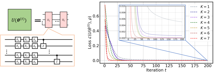
Figure 8: The implementation of the quantum encoder and the training loss of QAE. The left panel illustrates the quantum gates arrangement to compose $U_{l}(\bm{\theta})$ employed in the quantum encoder. The trainable parameters are contained in the rotational single qubit gates RZ and RY. The right panel demonstrates the training loss of the QAE-based fidelity estimator in the first stage. The label ‘$K=x$ refers to the employed number of latent qubits of the QAE-based fidelity estimator is $x$.

We further evaluate the performance of the QAE-based fidelity estimator to estimate $\operatorname{F}(\rho,\rho)=1$, where $\rho$ is a full-rank $8$-qubit states. Specifically, the construction of $\rho$ follows Eqn. (53), i.e., $\rho=\mathcal{N}(\ket{\Psi^{(1)}},p=0.5,r=2^{8},a=1/10)$. The implementation of the quantum encoder $U(\bm{\theta})$ and all hyper-parameters settings such as the layer number, the learning rate, the varied number of latent qubits, and the number of iterations, are exactly same with those used in the main text.

The simulation results are illustrated in Figure 9. The left panel shows the training loss of QAE with respect to the different $K$. An empirical observation is that a larger $K$ ensures a lower loss $\delta$. This phenomenon is caused by the following facts. First, since the input state is full rank and incompressible by QAE, some information in $\rho$ must be lost in the compressed state $\sigma$ when QAE with $2^{K}<r^{*}$ is applied to compress $\rho$. Second, increasing $K$ enables $\sigma$ to preserve more information in $\rho$ and reduce the training error $\delta$. The right panel depicts the estimated fidelity bounds of the QAE-based fidelity estimator, the SSFB, and the exact result. The achieved results accord with Theorem 2, where a smaller $\delta$ ensures a lower estimation error. Moreover, even though the input state is full-rank, the QAE-based fidelity estimator outperforms SSFB when $K>4$. Such a result indicates the applicability of our proposal on NISQ devices.

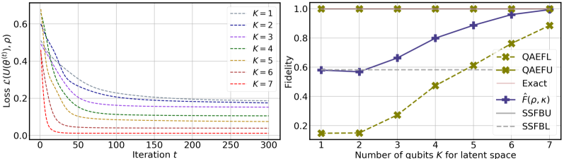
Figure 9: The simulation results for the fidelity estimation. The left panel demonstrates the training loss of the QAE-based fidelity estimator in the first stage when it applies to estimate $\operatorname{F}(\rho,\rho)$. The right panel illustrates the estimated fidelity bounds and SSFB. The meaning of labels is identical to those in Figure 1 and Figure 8.

Appendix E The resource-efficient QAE-based fidelity estimator

Let us recall the machinery of the QAE-based fidelity estimator introduced above. In the third step, e.g., Figure 2(iii), the destructive Swap test subacsi2019entanglement is exploited to estimate $W_{ij}$ in Eqn. (49). However, the employment of this strategy will doubly increase the required number of qubits to conduct the fidelity estimation, which is resource-unfriendly to NISQ devices. In this section, we devise a resource-efficient QAE-based fidelity estimator to fully exploit the available quantum resource. Namely, when $\rho$ and $\kappa$ are two low-rank $N$-qubit states, $N$ qubits are sufficient to estimate the fidelity $\operatorname{F}(\rho,\kappa)$ within a tolerable error. For ease of description, here we suppose that the rank for both states $\rho$ and $\kappa$ is $r^{*}$. Note that our results can be easily generalized to the scenario such that the rank of $\rho$ and $\kappa$ is distinct.

The only modification of the resource-efficient QAE-based fidelity estimator compared with the protocol as shown in Figure 2 is the third step, i.e., the way to collect $\widehat{W}$ in Eqn. (13), since the rest three steps do not use quantum devices or use at most $N$ qubits. To be more specific, we utilize QAE to estimate $W$ defined in Eqn. (49) instead of using the destructive Swap test. Following the same routine of the first step in Figure 2, we can apply QAE to collect the spectral information of $\kappa$, guaranteed by its low-rank property. Denote the estimated eigenvalues of $\kappa$ as $\{\hat{\mu}_{k}\}_{k=1}^{r}$, where $r$ may be not equal to $r^{*}$ in the non-optimal setting. Analogous to the preparation of $\ket{\hat{\varphi}_{i}}$ in Eqn. (12), the trained quantum encoder $U(\hat{\bm{a}})$ and the eigenvectors $\{\ket{\bm{b}_{k}}\}$ can be employed to prepare quantum states $\{\ket{\hat{\Phi}_{k}}\}_{k=1}^{r}$ that occupy the same subspace spanned by the eigenvectors of $\kappa$, i.e., $\ket{\hat{\Phi}_{k}}=U(\hat{\bm{a}})^{\dagger}\ket{0}^{\otimes N-K}\ket{\bm{b}_{k}}$. Given access to $\{\ket{\hat{\varphi}_{i}}\}$, $\{\hat{\mu}_{k}\}_{k=1}^{r}$, and $\{\ket{\hat{\Phi}_{k}}\}_{k=1}^{r}$, estimates the elements of $W$ in Eqn. (49) is estimated by

$$\widetilde{W}_{i,j}=\sum_{k=1}^{r}\hat{\mu}_{k}\sqrt{\hat{\lambda}_{i}\hat{\lambda}_{j}}\langle\hat{\varphi_{i}}|\hat{\Phi}_{k}\rangle\langle\hat{\Phi}_{k}|\hat{\varphi_{j}}\rangle.$$ (57)

Note that the computation of the inner product of two pure states, i.e., $\langle\hat{\varphi_{i}}|\hat{\Phi}_{k}\rangle$ or $\langle\hat{\Phi}_{k}|\hat{\varphi_{j}}\rangle$, can be accomplished by using $N$ qubits. To this end, it is sufficient to use $N$ qubits to calculate the matrix $\widetilde{W}$ and then compute the estimated fidelity $\widetilde{\text{F}}(\rho,\kappa)=\operatorname{Tr}(\sqrt{\widetilde{W}})$ based on Eqn. (50). Compared with previous proposals that employ at least $2N+1$ qubits to estimate $\operatorname{F}(\rho,\kappa)$, the modified QAE-based fidelity estimator is the optimal solution in the measure of qubits conut.

We end this subsection by analyzing the estimation error of the resource-efficient QAE-based fidelity estimator.

Lemma 7.

Suppose that the training loss of QAE in Eqn. (1) yields $\mathcal{L}(U(\bm{\theta}^{(T)}),\rho)=\delta_{1}$ and $\mathcal{L}(U(\bm{a}^{(T)}),\kappa)=\delta_{2}$. Let $\delta=\max\{\delta_{1},\delta_{2}\}$. Then the resource-efficient QAE-based fidelity estimator returns an estimated fidelity $\operatorname{\widetilde{F}}(\rho,\kappa)$ satisfying

$$\operatorname{\widetilde{F}}(\rho,\kappa)-\sqrt{2\delta}\leq\operatorname{F}(\rho,\kappa)\leq\operatorname{\widetilde{F}}(\rho,\kappa)+\sqrt{2\delta}.$$ (58)

Proof of Lemma 7.

The proof mainly follows the same routine of Theorem 2. Define the reconstructed state of $\kappa$ as

$$\hat{\kappa}=\sum_{k=1}^{r}\hat{\mu}_{k}|\hat{\Phi}_{k}\rangle\langle\hat{\Phi}_{k}|,$$ (59)

where $\{\hat{\mu}_{k}\}$ refers to the eigenvalues of the compressed state of $\kappa$ and $\{|\hat{\Phi}_{k}\rangle\}$ is defined in Eqn. (57).

We now quantify the estimation error of the proposed method. Mathematically, we derive the upper bound of $|\widetilde{\operatorname{F}}(\rho,\kappa)-\operatorname{F}(\rho,\kappa)|$, i.e.,

$$\left|\widetilde{\operatorname{F}}(\rho,\kappa)-\operatorname{F}(\rho,\kappa)\right|$$

$$= \left|\operatorname{F}(\hat{\rho},\hat{\kappa})-\operatorname{F}(\hat{\rho},\kappa)+\operatorname{F}(\hat{\rho},\kappa)-\operatorname{F}(\rho,\kappa)\right|$$

$$\leq \left|\operatorname{F}(\hat{\rho},\hat{\kappa})-\operatorname{F}(\hat{\rho},\kappa)\right|+\left|\operatorname{F}(\hat{\rho},\kappa)-\operatorname{F}(\rho,\kappa)\right|$$

$$\leq \operatorname{Tr}(|\hat{\kappa}-\kappa|)+\operatorname{Tr}(|\hat{\rho}-\rho|)$$

$$\leq \sqrt{2\delta_{1}}+\sqrt{2\delta_{2}}$$

$$\leq 2\sqrt{2\delta},$$ (60)

where the first inequality uses the triangle inequality, the second inequality employs the result of Lemma 5 (see Eqn. (C) for details), the third inequality exploits the Proposition 1, i.e., $\operatorname{Tr}(|\hat{\kappa}-\kappa|)=\delta_{1}$ and $\operatorname{Tr}(|\hat{\rho}-\rho|)=\delta_{1}$, and the last inequality comes from the definition $\delta=\max\{\delta_{1},\delta_{2}\}$. ∎

Appendix F The QAE-based quantum Gibbs state solver

In this section, we first review the implementation of the original variational quantum Gibbs state solver proposed by wang2020variational in Subsection F.1. We next present more simulation details about the QAE-based variational quantum Gibbs state solver in Subsection F.2.

F.1 Original variational quantum Gibbs state solver

Recall that a central idea in the variational quantum Gibbs states solver is replacing the von Neumann entropy $S(\rho(\bm{\gamma}))$ by its $R$-truncated version to simplify optimization wang2020variational . In doing so, the modified free energy, as so-called the $R$-truncated free energy, yields

$$\mathcal{F}_{R}(\rho(\bm{\gamma})):=\operatorname{Tr}(H\rho(\bm{\gamma}))-\frac{1}{\beta}S_{R}(\rho(\bm{\gamma}))=\operatorname{Tr}(H\rho(\bm{\gamma}))-\frac{1}{\beta}\sum_{j=0}^{R}C_{j}\operatorname{Tr}(\rho(\bm{\gamma})^{j+1}),$$ (61)

where $H$ is the specified Hamiltonian in Eqn. (16), $\beta=1/k_{B}T$ is the inverse temperature with $k_{B}$ being the Boltzmann constant, $C_{0}=\sum_{k=1}^{R}1/k$, $C_{j}=\sum_{k=j}^{R}{k\choose j}(-1)^{j}/k$ for $\forall j\in\{1,...,R-1\}$, $C_{R}=(-1)^{R}/R$. The goal of the variational quantum Gibbs states solver is continuously updating $\bm{\gamma}$ to minimize $\mathcal{F}_{R}(\rho(\bm{\gamma}))$, where the achieved state $\rho(\bm{\gamma}^{*})=\arg\min_{\rho(\bm{\gamma})}\mathcal{F}_{R}$ can well approximate the state $\rho_{G}$ in Eqn. (16).

The study wang2020variational explores the lower bound of the fidelity between the approximated state $\rho(\bm{\gamma})$ and the oriented state $\rho_{G}$ when the optimization is not optimal. Specifically, denote the the optimized parameters returned by the variational quantum Gibbs solver as $\bm{\hat{\gamma}}$, which satisfies

$$\mathcal{F}_{R}(\rho(\hat{\bm{\gamma}}))\leq\min_{\bm{\gamma}}\mathcal{F}_{R}(\rho(\bm{\gamma}))+\epsilon_{1},$$ (62)

where $\epsilon_{1}$ refers to the tolerable error. Then the following proposition summarizes the lower bound of $\operatorname{F}(\rho(\hat{\bm{\gamma}}),\rho_{G})$.

Proposition 2 (Theorem 1, wang2020variational ).

Following notation in Eqn. (62), let $\hat{\bm{\gamma}}$ be the optimized parameters and $r$ be the rank of $\rho(\hat{\bm{\gamma}})$. Denote $\epsilon_{1}$ as the tolerable error. The fidelity between the approximated state $\rho(\hat{\bm{\gamma}})$ and the oriented state $\rho_{G}$ is lower bounded by

$$\operatorname{F}(\rho(\hat{\bm{\gamma}}),\rho_{G})\geq 1-\sqrt{2\beta\epsilon},$$ (63)

where $\epsilon=\epsilon_{1}+\frac{2r}{R+1}(1-\Delta)^{R+1}$ and $\Delta\in(0,e^{-1})$ is a constant determined by the truncation number $R$.

F.2 More simulation details

The implementation of the QAE-based variational quantum Gibbs state solver. In numerical simulations, we apply the QAE-based variational quantum Gibbs state solver to prepare the quantum Gibbs state of the Ising chain model. In particular, let the Ising Hamiltonian be $H_{B}=-\sum_{i=1}^{I}Z_{i}Z_{i+1}$ with $I=3$, $Z_{I+1}=Z_{1}$, and $Z_{i}$ being the Pauli-Z matrix. The target quantum Gibbs state is

$$\rho_{G}=\frac{e^{-\beta H_{B}}}{\operatorname{Tr}(e^{-\beta H_{B}})}\in\mathbb{C}^{2^{3}\times 2^{3}}.$$ (64)

We follow the construction rule in wang2020variational to implement the variational quantum circuit $U(\bm{\gamma})$. Specifically, to generate the mixed state $\rho(\bm{\gamma})$, the unitary $U(\bm{\gamma})$ is applied to a $4$-qubit state $\ket{0}_{A}\ket{000}_{B}$, where the subscripts $A$ and $B$ refer to two subsystems. After interaction, the subsystem $A$ is traced out, i.e.,

$$\rho(\bm{\gamma})=\operatorname{Tr}_{A}(U(\bm{\gamma})(\ket{0}_{A}\ket{000}_{B})(\bra{0}_{A}\bra{000}_{B})U(\bm{\gamma})^{\dagger}).$$ (65)

Hyper-parameters settings. The variational quantum circuits $U(\bm{\gamma})$ and $U(\bm{\theta})$, which are used to prepare the variational quantum Gibbs state $\rho(\bm{\gamma})$ and to build the quantum encoder respectively, follow the hardware-efficient ansatz in Eqn. (54). Specifically, for the variational quantum circuit $U(\bm{\gamma})$, its layer number is set as $L=5$ and the learning rate to update $\bm{\gamma}$ is $\eta=0.2$. For the variational quantum circuits $U(\bm{\theta})$, its layer number is set as $L=4$ and the learning rate to update $\bm{\theta}$ is $\eta=0.2$. The number of latent qubits in QAE is set as $K=2$. The total number of iterations to optimize $\bm{\theta}$ is $100$. The parameters $\bm{\gamma}$ and $\bm{\theta}$ are initialized from a uniform distribution in $[0,2\pi)$ with the random seed $1$.

Appendix G Proof of Lemma 3

Before elaborating on the proof of Lemma 3, we first introduce three lemmas that will be exploited later. In particular, the first lemma (i.e., Lemma 9) enables us to connect the relative entropy with the fidelity. The second lemma (i.e., Lemma 8) quantifies the difference between the exact free energy $\mathcal{F}(\rho(\hat{\bm{\gamma}}))$ and the $R$-truncated free energy $\mathcal{F}_{R}(\rho(\hat{\bm{\gamma}}))$. The third lemma (i.e., Lemma 10), whose proof is shown in Subsection G.1, provides an upper bound of the difference between the accurate $R$-truncated free energy and the estimated $R$-truncated free energy achieved by QAE.

Lemma 8 (Lemma 2, wang2020variational ).

Given quantum states $\rho$ and $\kappa$ and a constant $\epsilon_{2}$, suppose that the relative entropy $S(\rho||\kappa)$ is less than $\epsilon_{2}$. Then the fidelity between $\rho$ and $\kappa$ satisfies

$$\operatorname{F}(\rho,\kappa)\geq 1-\sqrt{2S(\rho||\kappa)}\geq 1-\sqrt{2\epsilon_{2}}.$$ (66)

Lemma 9 (Lemma 4, wang2020variational ).

Define $\epsilon_{3}=|\mathcal{F}(\rho(\hat{\bm{\gamma}}))-\mathcal{F}_{R}(\rho(\hat{\bm{\gamma}}))|$. Let $\Delta$ be a constant such that $-\Delta\ln(\Delta)<\frac{1}{R+1}(1-\Delta)^{R+1}$ and $r$ be the rank of $\rho(\hat{\bm{\gamma}})$. Then the truncated error $\epsilon_{3}$ is upper bounded in the sense that

$$\epsilon_{3}\leq\frac{r}{R+1}(1-\Delta)^{R+1}.$$ (67)

Lemma 10.

Suppose that the training loss of QAE is $\delta$ given the input state $\rho(\bm{\gamma})$. Define $C_{\max}=\max_{j}C_{j}$ for $\forall j\in[R]$. The discrepancy between the $R$-truncated free energy $\mathcal{F}_{R}(\rho(\bm{\gamma}))$ and its estimation $\hat{\mathcal{F}}_{R}(\rho(\bm{\gamma}))$ achieved by QAE follows

$$\left|\mathcal{F}_{R}(\rho(\bm{\gamma}))-\hat{\mathcal{F}}_{R}(\rho(\bm{\gamma}))\right|\leq\frac{2C_{\max}\delta}{\beta(1-2\delta)}.$$ (68)

We are now ready to prove Lemma 3 by using the above three lemmas.

Proof of Lemma 3.

Supported by Lemma 8, we have

$$\operatorname{F}(\rho_{G},\rho(\hat{\bm{\gamma}}))\geq 1-\sqrt{2S(\rho(\hat{\bm{\gamma}})||\rho_{G})}.$$ (69)

In other words, the lower bound of $\operatorname{F}(\rho_{G},\rho(\hat{\bm{\gamma}}))$ can be achieved by deriving the upper bound of $S(\rho(\hat{\bm{\gamma}})||\rho_{G})$. Specifically, we have

$$S(\rho(\hat{\bm{\gamma}})||\rho_{G})= \beta|\mathcal{F}(\rho(\hat{\bm{\gamma}}))-\mathcal{F}(\rho_{G})|$$

$$= \beta\left|\mathcal{F}(\rho(\hat{\bm{\gamma}}))-\mathcal{F}_{R}(\rho(\hat{\bm{\gamma}}))+\mathcal{F}_{R}(\rho(\hat{\bm{\gamma}}))-\mathcal{F}(\rho_{G})\right|$$

$$\leq \beta\left|\mathcal{F}(\rho(\hat{\bm{\gamma}}))-\mathcal{F}_{R}(\rho(\hat{\bm{\gamma}}))\right|+\beta\left|\mathcal{F}_{R}(\rho(\hat{\bm{\gamma}}))-\mathcal{F}(\rho_{G})\right|$$

$$\leq \beta\frac{r}{R+1}(1-\Delta)^{R+1}+\beta\left|\mathcal{F}_{R}(\rho(\hat{\bm{\gamma}}))-\hat{\mathcal{F}}_{R}(\rho(\hat{\bm{\gamma}}))+\hat{\mathcal{F}}_{R}(\rho(\hat{\bm{\gamma}}))-\mathcal{F}(\rho_{G})\right|$$

$$\leq \beta\frac{r}{R+1}(1-\Delta)^{R+1}+\beta\epsilon_{1}+\beta\frac{2C_{\max}\delta}{\beta(1-2\delta)},$$ (70)

where the first inequality uses the triangle inequality, the second inequality uses the result of Lemma 9, i.e., $|\mathcal{F}_{R}(\rho(\hat{\bm{\gamma}}))-\mathcal{F}(\rho_{G})|\leq\epsilon_{3}$, and the last inequality exploits $|\hat{\mathcal{F}}_{R}(\rho(\hat{\bm{\gamma}}))-\mathcal{F}(\rho_{G})|\leq\epsilon_{1}$ and the result of Lemma 10.

In conjunction with Eqns. (69) and (G), we achieve the lower bound of $\operatorname{F}(\rho_{G},\rho(\hat{\bm{\gamma}}))$, which is

$$\operatorname{F}(\rho_{G},\rho(\hat{\bm{\gamma}}))\geq 1-\sqrt{2\beta\frac{r}{R+1}(1-\Delta)^{R+1}+2\beta\epsilon_{1}+\frac{4C_{\max}\delta}{1-2\delta}}.$$ (71)

∎

G.1 Proof of Lemma 10

Proof of Lemma 10.

Following Eqn. (61), the explicit form of the difference between $\mathcal{F}_{R}(\rho(\bm{\gamma}))$ and $\hat{\mathcal{F}}_{R}(\rho(\bm{\gamma}))$ yields

$$\left|\mathcal{F}_{R}(\rho(\bm{\gamma}))-\hat{\mathcal{F}}_{R}(\rho(\bm{\gamma}))\right|$$

$$= \left|\operatorname{Tr}(H\rho(\bm{\gamma}))-\frac{1}{\beta}\sum_{j=0}^{R}C_{j}\operatorname{Tr}(\rho(\bm{\gamma})^{j+1})-\operatorname{Tr}(H\rho(\bm{\gamma}))+\frac{1}{\beta}\sum_{j=0}^{R}C_{j}\operatorname{Tr}(\hat{\rho}(\bm{\gamma})^{j+1})\right|$$

$$= \left|\frac{1}{\beta}\sum_{j=0}^{R}C_{j}\operatorname{Tr}(\rho(\bm{\gamma})^{j+1})-\operatorname{Tr}(\hat{\rho}(\bm{\gamma})^{j+1})\right|$$

$$\leq \frac{1}{\beta}\sum_{j=0}^{R}C_{j}\left|\operatorname{Tr}\left(\rho(\bm{\gamma})^{j+1}-\hat{\rho}(\bm{\gamma})^{j+1}\right)\right|,$$ (72)

where $C_{j}$ is defined in Eqn. (61).

Recall the result of Lemma 5. When the training loss of QAE is $\delta$ for the input state $\rho(\bm{\gamma})$, we have

$$\operatorname{Tr}(|\rho(\bm{\gamma})-\hat{\rho}(\bm{\gamma})|)=2\delta.$$ (73)

By leveraging Eqn. (73), the upper bound in Eqn. (G.1) can be rewritten as

$$\left|\mathcal{F}_{R}(\rho(\bm{\gamma}))-\hat{\mathcal{F}}_{R}(\rho(\bm{\gamma}))\right|$$

$$\leq \frac{1}{\beta}\sum_{j=0}^{R}C_{j}\left|\operatorname{Tr}\left(\rho(\bm{\gamma})^{j+1}-\hat{\rho}(\bm{\gamma})^{j+1}\right)\right|$$

$$\leq \frac{1}{\beta}C_{\max}\sum_{j=0}^{R}(2\delta)^{j+1}$$

$$\leq \frac{2C_{\max}\delta}{\beta(1-2\delta)},$$ (74)

where the second inequality employs the fact $\operatorname{Tr}\left(\rho(\bm{\gamma})^{j+1}-\hat{\rho}(\bm{\gamma})^{j+1}\right)\leq\delta^{j+1}$ and the last inequality uses $\sum_{j=0}^{R}x^{j}\leq\frac{1}{1-x}$ for $x\in(0,1)$. ∎

Appendix H The QAE-based QFI estimator

In this section, we provide implementation and simulation details about the QAE-based QFI estimator. First, in Subsection H.1, we review the implementation of the original variational QFI estimator beckey2020variational . Next, we present more numerical simulation details about our proposal in Subsection H.2.

H.1 Variational QFI estimator

Let us illustrate an example to facilitate the understanding of quantum metrology. In the qubit-based magnetic field sensor, a probe quantum state $\rho$ is interacted with a source, i.e., a magnetic field whose information is described by a parameter $\vartheta$ koczor2020variational . After interaction, the information of the magnetic field, or equivalently, the parameter $\vartheta$, is encoded as the relative phase of the probe state, where the resultant quantum state is $\rho_{\vartheta}$. Meanwhile, the information about $\vartheta$ can then be extracted via a Ramsey-type measurement degen2017quantum . As introduced in the main text, the ultimate precision $\Delta\vartheta$ of a quantum sensing protocol is determined by the quantum fisher information (QFI) $\mathcal{I}(\vartheta,\rho_{\vartheta})$, i.e.,

$$(\Delta\vartheta)^{2}\geq\frac{1}{\nu\mathcal{I}(\vartheta,\rho_{\vartheta})},$$ (75)

where $\nu$ is the number of measurements.

Due to the computational hardness of acquiring $\mathcal{I}(\vartheta,\rho_{\vartheta})$, an alternative strategy is approximating this quantity by

$$\mathcal{I}_{\tau}(\vartheta;\rho_{\vartheta})=8\frac{1-\operatorname{F}(\rho_{\vartheta},\rho_{\vartheta+\tau})}{\tau^{2}},$$ (76)

where the fidelity $\operatorname{F}(\rho_{\vartheta},\rho_{\vartheta+\tau})$ measures the sensitivity of the probe state $\rho$ with respect to the small changes of the source (i.e., the source parameter drifts from $\vartheta$ to $\vartheta+\tau$). As indicated in Eqns. (75) and (76), a high sensitivity of the probe state, which results in a low fidelity $\operatorname{F}(\rho_{\vartheta},\rho_{\vartheta+\tau})$, ensures a large QFI and therefore a better precision $\Delta\vartheta$.

The above explanation reflects the significance of selecting a proper probe state $\rho$. Concretely, a probe state with a low fidelity $\operatorname{F}(\rho_{\vartheta},\rho_{\vartheta+\tau})$ allows a better performance of quantum sensing protocols over the one with the high fidelity. Although theoretical studies demonstrate that certain coherent or entanglement states are best choice, the preparation of such states on NISQ machines is extremely challenged, due to the unavoidable system noise. To conquer this issue, Beckey et al. proposed the variational QFI estimator beckey2020variational to actively learn a probe state that maximizes $\mathcal{I}_{\tau}(\vartheta,\rho_{\vartheta})$ adapting the system noise. In particular, the variational QFI estimator employs the variational quantum circuit $U(\bm{\gamma})$ to generate the probe state $\rho(\bm{\gamma})$. The aim of their proposal is seeking optimal parameters maximizing the corresponding QFI, i.e.,

$$\bm{\gamma}^{*}=\arg\max_{\bm{\gamma}}\mathcal{I}_{\tau}(\vartheta,\rho_{\vartheta}(\bm{\gamma})).$$ (77)

The updating rule at the $t$-th iteration follows

$$\bm{\gamma}^{(t+1)}=\bm{\gamma}^{(t)}+\eta\frac{\partial\mathcal{I}_{\tau}(\vartheta,\rho_{\vartheta}(\bm{\gamma}^{(t)}))}{\partial\bm{\gamma}},$$ (78)

where the gradients ${\partial\mathcal{I}_{\tau}(\vartheta,\rho_{\vartheta}(\bm{\gamma}^{(t)}))}/{\partial\bm{\gamma}}$ can be obtained via the parameter shift rule or be approximated by zeroth-order gradients methods.

Recall that the explicit form of $\mathcal{I}_{\tau}(\vartheta,\rho_{\vartheta}(\bm{\gamma}))$ in Eqn. (76) contains the term $\operatorname{F}(\rho_{\vartheta}(\bm{\gamma}),\rho_{\vartheta+\tau}(\bm{\gamma}))$, which is difficult to calculate cerezo2020variational . To tackle this issue, the variational QFI estimator employs the variational fidelity estimation solver in Appendix D.1 and SSFB in Appendix D.2 to estimate this quantity instead of computing $\operatorname{F}(\rho_{\vartheta}(\bm{\gamma}),\rho_{\vartheta+\tau}(\bm{\gamma}))$ analytically. As proved in beckey2020variational , the estimated QFI at the $t$-th iteration is lower bound by

$$\mathcal{I}_{\tau}(\vartheta,\rho_{\vartheta}(\bm{\gamma}))\geq 8\frac{1-\max\{\operatorname{F}_{U}(\rho_{\vartheta}(\bm{\gamma}),\rho_{\vartheta+\tau}(\bm{\gamma})),\operatorname{\widehat{F}_{\bigtriangleup}}(\bm{\theta}),\rho_{\vartheta+\tau}(\bm{\gamma}))\}}{\tau^{2}}.$$ (79)

H.2 Simulation details

The implementation of the QAE-based QFI estimator. In numerical simulations, we follow the construction rule in beckey2020variational to implement the variational quantum circuit $U(\bm{\gamma})$. Specifically, the unitary $U(\bm{\gamma})$ is applied to a $4$-qubit state $\ket{0}^{\otimes 4}$ to generate the state $\rho(\bm{\gamma})=U(\bm{\gamma})(\ket{0}\bra{0})^{\otimes 4}U(\bm{\gamma})^{\dagger}$. Subsequently, the state is interacting with the unitary $W(\vartheta)=e^{i\vartheta G}$ with $G=\sum_{i=1}^{3}Z_{i}$ and $\vartheta=0.1$ to prepare the state $\rho_{\vartheta}(\bm{\gamma})=W(\vartheta)\rho(\bm{\gamma})W(\vartheta)^{\dagger}$.

Hyper-parameters settings. The variational quantum circuits $U(\bm{\gamma})$ and $U(\bm{\theta})$, which are used to prepare the probe state $\rho_{\vartheta}(\bm{\gamma})$ and to build the quantum encoder respectively, follow the hardware-efficient ansatz in Eqn. (54). Specifically, for the variational quantum circuit $U(\bm{\gamma})$, its layer number is set as $L=5$ and the learning rate to update $\bm{\gamma}$ is $\eta=0.01$. For the variational quantum circuits $U(\bm{\theta})$, its layer number is set as $L=4$ and the learning rate to update $\bm{\theta}$ is $\eta=0.1$. The number of latent qubits in QAE is set as $K=2$. The total number of iterations to optimize $\bm{\theta}$ is $200$. The parameters $\bm{\gamma}$ and $\bm{\theta}$ are initialized from a uniform distribution in $[0,2\pi)$ with the random seed $1$.

Appendix I Proof of Lemma 4

Proof of Lemma 4.

The results shown in Lemma 4 can be easily obtained by leveraging Theorem 2. Recall the explicit form of the estimated QFI, i.e.,

$$\hat{\mathcal{I}}_{\tau}(\vartheta,\rho_{\vartheta}(\bm{\gamma}))=8\frac{1-\operatorname{\widehat{F}}(\rho_{\vartheta}(\bm{\gamma}),\rho_{\vartheta+\tau}(\bm{\gamma}))}{\tau^{2}}.$$ (80)

Combining the above equation with Eqn. (44), we have

$$\begin{cases}\hat{\mathcal{I}}_{\tau}(\vartheta,\rho_{\vartheta}(\bm{\gamma}))\leq 8\frac{1-\operatorname{F}(\rho_{\vartheta}(\bm{\gamma}),\rho_{\vartheta+\tau}(\bm{\gamma}))+\sqrt{2\delta}}{\tau^{2}}=\mathcal{I}_{\tau}(\vartheta,\rho_{\vartheta}(\bm{\gamma}))+\frac{8\sqrt{2\delta}}{\tau^{2}}\\ \hat{\mathcal{I}}_{\tau}(\vartheta,\rho_{\vartheta}(\bm{\gamma}))\geq 8\frac{1-\operatorname{F}(\rho_{\vartheta}(\bm{\gamma}),\rho_{\vartheta+\tau}(\bm{\gamma}))-\sqrt{2\delta}}{\tau^{2}}=\mathcal{I}_{\tau}(\vartheta,\rho_{\vartheta}(\bm{\gamma}))-\frac{8\sqrt{2\delta}}{\tau^{2}}.\end{cases}$$ (81)

After simplification, we have

$$\hat{\mathcal{I}}_{\tau}(\vartheta,\rho_{\vartheta}(\bm{\gamma}))-\frac{8\sqrt{2\delta}}{\tau^{2}}\leq\mathcal{I}_{\tau}(\vartheta,\rho_{\vartheta}(\bm{\gamma}))\leq\hat{\mathcal{I}}_{\tau}(\vartheta,\rho_{\vartheta}(\bm{\gamma}))+\frac{8\sqrt{2\delta}}{\tau^{2}}.$$ (82)

∎

References

• (1) Jacob Biamonte, Peter Wittek, Nicola Pancotti, Patrick Rebentrost, Nathan Wiebe, and Seth Lloyd. Quantum machine learning. Nature, 549(7671):195, 2017.
• (2) Juan Carrasquilla and Roger G Melko. Machine learning phases of matter. Nature Physics, 13(5):431, 2017.
• (3) Keith T Butler, Daniel W Davies, Hugh Cartwright, Olexandr Isayev, and Aron Walsh. Machine learning for molecular and materials science. Nature, 559(7715):547–555, 2018.
• (4) Jeongwan Haah, Aram W Harrow, Zhengfeng Ji, Xiaodi Wu, and Nengkun Yu. Sample-optimal tomography of quantum states. IEEE Transactions on Information Theory, 63(9):5628–5641, 2017.
• (5) Leonid Gurvits. Classical deterministic complexity of edmonds’ problem and quantum entanglement. In Proceedings of the thirty-fifth annual ACM symposium on Theory of computing, pages 10–19, 2003.
• (6) Scott Aaronson and Guy N Rothblum. Gentle measurement of quantum states and differential privacy. arXiv preprint arXiv:1904.08747, 2019.
• (7) Scott Aaronson. Shadow tomography of quantum states. SIAM Journal on Computing, 49(5):STOC18–368, 2019.
• (8) Hsin-Yuan Huang, Richard Kueng, and John Preskill. Predicting many properties of a quantum system from very few measurements. Nature Physics, 16(10):1050–1057, 2020.
• (9) David Gross, Yi-Kai Liu, Steven T Flammia, Stephen Becker, and Jens Eisert. Quantum state tomography via compressed sensing. Physical review letters, 105(15):150401, 2010.
• (10) Lee A Rozema, Dylan H Mahler, Alex Hayat, Peter S Turner, and Aephraim M Steinberg. Quantum data compression of a qubit ensemble. Physical review letters, 113(16):160504, 2014.
• (11) A. Shabani, M. Mohseni, S. Lloyd, R. L. Kosut, and H. Rabitz. Estimation of many-body quantum hamiltonians via compressive sensing. Phys. Rev. A, 84:012107, Jul 2011.
• (12) Jonathan Romero, Jonathan P Olson, and Alan Aspuru-Guzik. Quantum autoencoders for efficient compression of quantum data. Quantum Science and Technology, 2(4):045001, 2017.
• (13) Chenfeng Cao and Xin Wang. Noise-assisted quantum autoencoder. Physical Review Applied, 15(5):054012, 2021.
• (14) Lucas Lamata, Unai Alvarez-Rodriguez, José David Martín-Guerrero, Mikel Sanz, and Enrique Solano. Quantum autoencoders via quantum adders with genetic algorithms. Quantum Science and Technology, 4(1):014007, 2018.
• (15) John Preskill. Quantum computing in the nisq era and beyond. Quantum, 2:79, 2018.
• (16) Alex Pepper, Nora Tischler, and Geoff J Pryde. Experimental realization of a quantum autoencoder: The compression of qutrits via machine learning. Physical review letters, 122(6):060501, 2019.
• (17) Chang-Jiang Huang, Hailan Ma, Qi Yin, Jun-Feng Tang, Daoyi Dong, Chunlin Chen, Guo-Yong Xiang, Chuan-Feng Li, and Guang-Can Guo. Realization of a quantum autoencoder for lossless compression of quantum data. Physical Review A, 102(3):032412, 2020.
• (18) Dmytro Bondarenko and Polina Feldmann. Quantum autoencoders to denoise quantum data. Physical Review Letters, 124(13):130502, 2020.
• (19) Xiao-Ming Zhang, Weicheng Kong, Muhammad Usman Farooq, Man-Hong Yung, Guoping Guo, and Xin Wang. Generic detection-based error mitigation using quantum autoencoders. Physical Review A, 103(4):L040403, 2021.
• (20) Carlos Bravo-Prieto. Quantum autoencoders with enhanced data encoding. Machine Learning: Science and Technology, 2021.
• (21) Michael A Nielsen and Isaac L Chuang. Quantum computation and quantum information. Cambridge University Press, 2010.
• (22) Jaroslaw Adam Miszczak, Zbigniew Puchała, Pawel Horodecki, Armin Uhlmann, and Karol Życzkowski. Sub–and super–fidelity as bounds for quantum fidelity. Quantum Information and Computation, 9(1&2):0103–0130, 2009.
• (23) Fernando GSL Brandao and Krysta M Svore. Quantum speed-ups for solving semidefinite programs. In 2017 IEEE 58th Annual Symposium on Foundations of Computer Science (FOCS), pages 415–426. IEEE, 2017.
• (24) David Poulin and Pawel Wocjan. Sampling from the thermal quantum gibbs state and evaluating partition functions with a quantum computer. Physical review letters, 103(22):220502, 2009.
• (25) Marco Cerezo, Alexander Poremba, Lukasz Cincio, and Patrick J Coles. Variational quantum fidelity estimation. Quantum, 4:248, 2020.
• (26) Ranyiliu Chen, Zhixin Song, Xuanqiang Zhao, and Xin Wang. Variational quantum algorithms for trace distance and fidelity estimation. arXiv preprint arXiv:2012.05768, 2020.
• (27) Ruslan Salakhutdinov and Geoffrey Hinton. Semantic hashing. International Journal of Approximate Reasoning, 50(7):969–978, 2009.
• (28) Chong Zhou and Randy C Paffenroth. Anomaly detection with robust deep autoencoders. In Proceedings of the 23rd ACM SIGKDD International Conference on Knowledge Discovery and Data Mining, pages 665–674, 2017.
• (29) Pascal Vincent, Hugo Larochelle, Yoshua Bengio, and Pierre-Antoine Manzagol. Extracting and composing robust features with denoising autoencoders. In Proceedings of the 25th international conference on Machine learning, pages 1096–1103, 2008.
• (30) Ian Goodfellow, Yoshua Bengio, and Aaron Courville. Deep learning. MIT press, 2016.
• (31) Marcello Benedetti, Erika Lloyd, Stefan Sack, and Mattia Fiorentini. Parameterized quantum circuits as machine learning models. Quantum Science and Technology, 4(4):043001, 2019.
• (32) Yuxuan Du, Min-Hsiu Hsieh, Tongliang Liu, and Dacheng Tao. Expressive power of parametrized quantum circuits. Phys. Rev. Research, 2:033125, Jul 2020.
• (33) Kosuke Mitarai, Makoto Negoro, Masahiro Kitagawa, and Keisuke Fujii. Quantum circuit learning. Physical Review A, 98(3):032309, 2018.
• (34) Kerstin Beer, Dmytro Bondarenko, Terry Farrelly, Tobias J Osborne, Robert Salzmann, Daniel Scheiermann, and Ramona Wolf. Training deep quantum neural networks. Nature Communications, 11(1):1–6, 2020.
• (35) Edward Farhi and Hartmut Neven. Classification with quantum neural networks on near term processors. arXiv preprint arXiv:1802.06002, 2018.
• (36) Shi-Jian Gu. Fidelity approach to quantum phase transitions. International Journal of Modern Physics B, 24(23):4371–4458, 2010.
• (37) Keisuke Fujii, Hirotada Kobayashi, Tomoyuki Morimae, Harumichi Nishimura, Shuhei Tamate, and Seiichiro Tani. Impossibility of classically simulating one-clean-qubit model with multiplicative error. Physical review letters, 120(20):200502, 2018.
• (38) Maria Schuld, Ville Bergholm, Christian Gogolin, Josh Izaac, and Nathan Killoran. Evaluating analytic gradients on quantum hardware. Physical Review A, 99(3):032331, 2019.
• (39) John A Smolin, Jay M Gambetta, and Graeme Smith. Efficient method for computing the maximum-likelihood quantum state from measurements with additive gaussian noise. Physical review letters, 108(7):070502, 2012.
• (40) Yiğit Subaşı, Lukasz Cincio, and Patrick J Coles. Entanglement spectroscopy with a depth-two quantum circuit. Journal of Physics A: Mathematical and Theoretical, 52(4):044001, 2019.
• (41) Marco Cerezo, Akira Sone, Tyler Volkoff, Lukasz Cincio, and Patrick J Coles. Cost function dependent barren plateaus in shallow parametrized quantum circuits. Nature communications, 12(1):1–12, 2021.
• (42) Yuxuan Du, Tao Huang, Shan You, Min-Hsiu Hsieh, and Dacheng Tao. Quantum circuit architecture search: error mitigation and trainability enhancement for variational quantum solvers. arXiv preprint arXiv:2010.10217, 2020.
• (43) Kaining Zhang, Min-Hsiu Hsieh, Liu Liu, and Dacheng Tao. Toward trainability of quantum neural networks. arXiv preprint arXiv:2011.06258, 2020.
• (44) John Watrous. Quantum Computational Complexity. Springer New York, New York, NY, 2009.
• (45) Norbert Schuch, Michael M Wolf, Frank Verstraete, and J Ignacio Cirac. Computational complexity of projected entangled pair states. Physical review letters, 98(14):140506, 2007.
• (46) Youle Wang, Guangxi Li, and Xin Wang. Variational quantum gibbs state preparation with a truncated taylor series. arXiv preprint arXiv:2005.08797, 2020.
• (47) Yuxuan Du, Min-Hsiu Hsieh, Tongliang Liu, Shan You, and Dacheng Tao. On the learnability of quantum neural networks. arXiv preprint arXiv:2007.12369, 2020.
• (48) Igor Lovchinsky, AO Sushkov, E Urbach, Nathalie P de Leon, Soonwon Choi, Kristiaan De Greve, R Evans, R Gertner, E Bersin, C Müller, et al. Nuclear magnetic resonance detection and spectroscopy of single proteins using quantum logic. Science, 351(6275):836–841, 2016.
• (49) L McCuller, C Whittle, D Ganapathy, K Komori, M Tse, A Fernandez-Galiana, L Barsotti, P Fritschel, M MacInnis, F Matichard, et al. Frequency-dependent squeezing for advanced ligo. Physical Review Letters, 124(17):171102, 2020.
• (50) Vittorio Giovannetti, Seth Lloyd, and Lorenzo Maccone. Quantum metrology. Physical review letters, 96(1):010401, 2006.
• (51) Vittorio Giovannetti, Seth Lloyd, and Lorenzo Maccone. Advances in quantum metrology. Nature photonics, 5(4):222, 2011.
• (52) Bálint Koczor, Suguru Endo, Tyson Jones, Yuichiro Matsuzaki, and Simon C Benjamin. Variational-state quantum metrology. New Journal of Physics, 2020.
• (53) Dénes Petz and Catalin Ghinea. Introduction to quantum fisher information. In Quantum probability and related topics, pages 261–281. World Scientific, 2011.
• (54) Jacob L Beckey, M Cerezo, Akira Sone, and Patrick J Coles. Variational quantum algorithm for estimating the quantum fisher information. arXiv preprint arXiv:2010.10488, 2020.
• (55) James Stokes, Josh Izaac, Nathan Killoran, and Giuseppe Carleo. Quantum natural gradient. Quantum, 4:269, 2020.
• (56) David Wierichs, Christian Gogolin, and Michael Kastoryano. Avoiding local minima in variational quantum eigensolvers with the natural gradient optimizer. Physical Review Research, 2(4):043246, 2020.
• (57) Suguru Endo, Simon C Benjamin, and Ying Li. Practical quantum error mitigation for near-future applications. Physical Review X, 8(3):031027, 2018.
• (58) Ying Li and Simon C Benjamin. Efficient variational quantum simulator incorporating active error minimization. Physical Review X, 7(2):021050, 2017.
• (59) Jarrod R McClean, Mollie E Kimchi-Schwartz, Jonathan Carter, and Wibe A De Jong. Hybrid quantum-classical hierarchy for mitigation of decoherence and determination of excited states. Physical Review A, 95(4):042308, 2017.
• (60) Kristan Temme, Sergey Bravyi, and Jay M Gambetta. Error mitigation for short-depth quantum circuits. Physical review letters, 119(18):180509, 2017.
• (61) Jarrod R McClean, Sergio Boixo, Vadim N Smelyanskiy, Ryan Babbush, and Hartmut Neven. Barren plateaus in quantum neural network training landscapes. Nature communications, 9(1):1–6, 2018.
• (62) Yuxuan Du, Zhuozhuo Tu, Xiao Yuan, and Dacheng Tao. An efficient measure for the expressivity of variational quantum algorithms. arXiv preprint arXiv:2104.09961, 2021.
• (63) He-Liang Huang, Yuxuan Du, Ming Gong, Youwei Zhao, Yulin Wu, Chaoyue Wang, Shaowei Li, Futian Liang, Jin Lin, Yu Xu, et al. Experimental quantum generative adversarial networks for image generation. arXiv preprint arXiv:2010.06201, 2020.
• (64) Yang Qian, Xinbiao Wang, Yuxuan Du, Xingyao Wu, and Dacheng Tao. The dilemma of quantum neural networks. arXiv preprint arXiv:2106.0497, 2021.
• (65) Maria Schuld and Nathan Killoran. Quantum machine learning in feature hilbert spaces. Physical review letters, 122(4):040504, 2019.
• (66) Yadong Wu, Juan Yao, Pengfei Zhang, and Hui Zhai. Expressivity of quantum neural networks. arXiv preprint arXiv:2101.04273.
• (67) Vojtěch Havlíček, Antonio D Córcoles, Kristan Temme, Aram W Harrow, Abhinav Kandala, Jerry M Chow, and Jay M Gambetta. Supervised learning with quantum-enhanced feature spaces. Nature, 567(7747):209, 2019.
• (68) Thomas Hubregtsen, David Wierichs, Elies Gil-Fuster, Peter-Jan HS Derks, Paul K Faehrmann, and Johannes Jakob Meyer. Training quantum embedding kernels on near-term quantum computers. arXiv preprint arXiv:2105.02276, 2021.
• (69) Takeru Kusumoto, Kosuke Mitarai, Keisuke Fujii, Masahiro Kitagawa, and Makoto Negoro. Experimental quantum kernel trick with nuclear spins in a solid. npj Quantum Information, 7(1):1–7, 2021.
• (70) Maria Schuld. Supervised quantum machine learning models are kernel methods. arXiv preprint arXiv:2101.11020, 2021.
• (71) Xinbiao Wang, Yuxuan Du, Yong Luo, and Dacheng Tao. Towards understanding the power of quantum kernels in the nisq era. arXiv preprint arXiv:2103.16774, 2021.
• (72) Koenraad MR Audenaert. Comparisons between quantum state distinguishability measures. arXiv preprint arXiv:1207.1197, 2012.
• (73) Ryan LaRose, Arkin Tikku, Étude O’Neel-Judy, Lukasz Cincio, and Patrick J Coles. Variational quantum state diagonalization. npj Quantum Information, 5(1):1–10, 2019.
• (74) Yuxuan Du, Min-Hsiu Hsieh, Tongliang Liu, and Dacheng Tao. A grover-search based quantum learning scheme for classification. New Journal of Physics, 2021.
• (75) Ryan LaRose and Brian Coyle. Robust data encodings for quantum classifiers. Physical Review A, 102(3):032420, 2020.
• (76) Yuto Takaki, Kosuke Mitarai, Makoto Negoro, Keisuke Fujii, and Masahiro Kitagawa. Learning temporal data with variational quantum recurrent neural network. arXiv preprint arXiv:2012.11242, 2020.
• (77) Christian L Degen, F Reinhard, and Paola Cappellaro. Quantum sensing. Reviews of modern physics, 89(3):035002, 2017.