Fractional dark energy: phantom behavior and negative absolute temperature

Abstract

The fractional dark energy (FDE) model describes the accelerated expansion of the Universe through a nonrelativistic gas of particles with a noncanonical kinetic term. This term is proportional to the absolute value of the three-momentum to the power of $3w$, where $w$ is simply the dark energy equation of state parameter, and the corresponding energy leads to an energy density that mimics the cosmological constant. In this paper we expand the fractional dark energy model considering a non-zero chemical potential and we show that it may thermodynamically describe a phantom regime. The Planck constraints on the equation of state parameter put upper limits on the allowed value of the ratio of the chemical potential to the temperature. In the second part, we investigate the system of fractional dark energy particles with negative absolute temperatures (NAT). NAT are possible in quantum systems and in cosmology, if there exists an upper bound on the energy. This maximum energy is one ingredient of the FDE model and indicates a connection between FDE and NAT, if FDE is composed of fermions. In this scenario, the equation of state parameter is equal to minus one and, using cosmological observations, we find that the transition from positive to negative temperatures is allowed at any redshift larger than one.

I Introduction

Observations of type-Ia supernovae (SNe) indicate that the Universe is currently undergoing a phase of accelerated expansion perlmutter1999 ; reiss1998 . A fluid with negative pressure, dark energy (DE), causes this expansion, but its nature is one of the major challenges in modern cosmology. The simplest candidate for DE is a cosmological constant, in agreement with most of the cosmological observations Aghanim:2018eyx . However, the existing tensions in the $\Lambda$CDM model, specially the one arising from the determination of the Hubble constant from cosmic microwave background (CMB) data Aghanim:2018eyx and its local measurement trough Cepheids Riess:2020fzl , summed to the lack of well-motivated explanations for the origin of such a constant leads to alternative candidates for DE. Among a plethora of options, there are scalar and vector fields peebles1988 ; ratra1988 ; Frieman1992 ; Frieman1995 ; Caldwell:1997ii ; Padmanabhan:2002cp ; Bagla:2002yn ; ArmendarizPicon:2000dh ; Brax1999 ; Copeland2000 ; Vagnozzi:2018jhn ; Koivisto:2008xf ; Bamba:2008ja ; Emelyanov:2011ze ; Emelyanov:2011wn ; Emelyanov:2011kn ; Kouwn:2015cdw ; Landim:2015upa ; Landim:2016dxh ; Banerjee:2020xcn , metastable DE Szydlowski:2017wlv ; Stachowski:2016zpq ; Stojkovic:2007dw ; Greenwood:2008qp ; Abdalla:2012ug ; Shafieloo:2016bpk ; Landim:2016isc ; Landim:2017kyz ; Landim:2017lyq , holographic DE Hsu:2004ri ; Li:2004rb ; Pavon:2005yx ; Wang:2005jx ; Wang:2005pk ; Wang:2005ph ; Wang:2007ak ; Landim:2015hqa ; Li:2009bn ; Li:2009zs ; Li:2011sd ; Saridakis:2017rdo ; Mamon:2017crm ; Mukherjee:2016lor ; Feng:2016djj ; Herrera:2016uci ; Forte:2016ben , interacting DE Wetterich:1994bg ; Amendola:1999er ; Guo:2004vg ; Cai:2004dk ; Guo:2004xx ; Bi:2004ns ; Gumjudpai:2005ry ; Yin:2007vq ; Costa:2013sva ; Abdalla:2014cla ; Costa:2014pba ; Landim:2015poa ; Landim:2015uda ; Costa:2016tpb ; Marcondes:2016reb ; Landim:2016gpz ; Wang:2016lxa ; Farrar:2003uw ; micheletti2009 ; Yang:2017yme ; Marttens:2016cba ; Yang:2017zjs ; Costa:2018aoy ; Yang:2018euj ; Landim:2019lvl ; Vagnozzi:2019kvw , models using extra dimensions dvali2000 , etc.

Recently, an alternative explanation for the cosmological constant was proposed in Landim:2021www , in the so-called fractional dark energy (FDE) model. In this setup, the energy of the system has a noncanonical kinetic term, proportional to $p^{3w}$, where $p$ is the three-momentum and $w$ is the DE equation of state parameter. The corresponding energy density is constant and mimics the one of the cosmological constant. Its smallness, however, is not a completely free parameter, but may arise from a Fermi-Dirac integral and it is related to the particle’s minimum energy. Furthermore, the energy eigenvalue is obtained from fractional quantum mechanics (see laskin2018fractional for a recent review on fractional quantum mechanics), where the Laplacian has a fractional power (leading to the Riesz integral). In fact, fractional calculus has been used in different contexts, such as in fractional quantum mechanics laskin2000fractional ; Laskin:2002zz ; guo2006some ; bayin2012consistency ; bayin2012comment ; dong2007some ; de2010fractional , Newtonian gravity Giusti:2020kcv ; Giusti:2020rul and quantum cosmology Moniz:2020emn ; Rasouli:2021lgy .

In this paper we further investigate the FDE model in two contexts. First, we analyze the influence of a non-zero chemical potential. In this scenario, the equation of state can be smaller than minus one, indicating a phantom behavior that comes only from the gas properties. Taking the measurements of $w$ from Planck into account Aghanim:2018eyx for the $w$CDM model, we are able to obtain upper limits for the ratio of the chemical potential to the temperature.

Since the FDE model has a maximum energy as an ingredient to avoid a divergence when the momentum goes to zero, it is natural to investigate whether FDE particles can have negative absolute temperatures (NAT). NAT were initially predicted and explored in the late 1940s and in the 1950s, both experimentally (in a crystal) purcell1951nuclear , and theoretically onsager1949statistical ; Ramsey:1956zz . They require an upper bound on the energy since the Boltzmann distribution function, for instance, would diverge if $T<0$ and the energy is unlimited Ramsey:1956zz ; klein1956negative . A revival of NAT occurred after the experimental realization of NAT for motional degrees of freedom braun2013negative , rather than the previously done localized spin systems purcell1951nuclear ; oja1997nuclear ; medley2011spin . In cosmology, an interesting consequence of negative temperatures is negative pressure, thus indicating a possible relation between DE and NAT. In Vieira:2016lyj , NAT in cosmology were further investigated. Hence, we explore the connection between NAT and the FDE model in the second part of this work and we use cosmological observations to investigate the transition from positive temperature to NAT.

This paper is organized in the following manner. In section II we review the FDE model. Section III is devoted to analyzing the system of FDE particles when the chemical potential is non-zero, while in section IV we investigate the connection between FDE and NAT. In section V we summarize the work and present our conclusions. We will use natural units $\hslash=c=k_{B}=1$ throughout the text, unless explicitly stated.

II Fractional dark energy

In this section we review the main features of the FDE model presented in Landim:2021www . FDE is composed of particles that satisfy the fractional Schrödinger equation. In the context of fractional calculus a fractional derivative can be defined as the Riemann-Liouville derivative oldham2006fractional

$${}_{a}D^{\alpha}_{x}f(x)=\frac{1}{\Gamma(n+1-\alpha)}\frac{d^{n+1}}{dx^{n+1}}\int^{x}_{a}(x-y)^{n-\alpha}f(y)dy\,,$$ (1)

for $n\leq\alpha<n+1$, where $\Gamma(n+1-\alpha)$ is the Gamma function. The inverse operator is the Riemann-Liouville fractional integration operator

$${}_{a}D^{-\alpha}_{x}f(x)=\frac{1}{\Gamma(\alpha)}\int^{x}_{a}(x-y)^{\alpha-1}f(y)dy\,,\quad\alpha>0\,,$$ (2)

such that ${}_{a}D^{\alpha}_{b}(_{a}D^{-\alpha}_{b}f(x))=f(x)$, with the operators satisfying the property ${}_{a}D^{\pm\alpha}_{b}(_{a}D^{\pm\beta}_{b}f(x))={}_{a}D^{\alpha\pm\beta}_{b}f(x)$.

The operator $(\hslash\nabla)^{\alpha}$ is thus defined as laskin2018fractional

$$(\hslash\nabla)^{\alpha}=-\frac{\hslash^{\alpha}}{2\cos(\pi\alpha/2)}\Big{[}_{-\infty}D^{\alpha}_{x}+_{x}D^{\alpha}_{\infty}\Big{]}\,,$$ (3)

where $\alpha$ is the Lévy index $1<\alpha\leq 2$.

The quantum Riesz fractional derivative (or integral, if $\alpha<0$) gives the fractional Laplacian operator

$$(-\hslash^{2}\Delta)^{\alpha/2}\psi(\mathbf{r},t)=\frac{1}{(2\pi\hslash)^{3}}\int d^{3}pe^{i\mathbf{p}\cdot\mathbf{r}/\hslash}|\mathbf{p}|^{\alpha}\varphi(\mathbf{p},t)\,.$$ (4)

Therefore, the fractional Schrödinger equation for FDE is

$$i\hslash\frac{\partial\psi(\mathbf{r},t)}{\partial t}=C(-\hslash^{2}\Delta)^{3w/2}\psi(\mathbf{r},t)\,,$$ (5)

where $C$ is a constant with units of $[C]=\text{erg}^{1-3w}$cm^3ws^-3w (or [energy]^1-3w, in natural units).

The eigenvalue of the Hamiltonian operator gives a noncanonical kinetic term, which can be inserted into the nonrelativistic limit of the energy-momentum relation

$$\epsilon\approx m+\frac{p^{2}}{2m}+\frac{C}{p^{-3w}}\,,$$ (6)

where $p\equiv|\mathbf{p}|$. When the non-relativistic particles cooled down below the rest mass ($Cp^{3w}>m$) the DE behavior started dominating.

The DE number density and energy density are then respectively given by

$$n= -\frac{C^{-\frac{1}{w}}g}{6\pi^{2}w}\int_{\epsilon_{\min}}^{\epsilon_{\max}}\frac{\epsilon^{\frac{1}{w}-1}}{e^{\beta\epsilon}\pm 1}d\epsilon\,,$$ (7)

$$= -\frac{C^{-\frac{1}{w}}g}{6\pi^{2}w}\beta^{-\frac{1}{w}}\mathscr{F}^{u_{\max}}_{u_{\min},\frac{1}{w}-1}\,,$$ (8)

$$\rho= -\frac{C^{-\frac{1}{w}}g}{6\pi^{2}w}\int_{\epsilon_{\min}}^{\epsilon_{\max}}\frac{\epsilon^{\frac{1}{w}}}{e^{\beta\epsilon}\pm 1}d\epsilon\,$$ (9)

$$= -\frac{C^{-\frac{1}{w}}g}{6\pi^{2}w}\beta^{-\frac{1+w}{w}}\mathscr{F}^{u_{\max}}_{u_{\min},\frac{1}{w}}\,,$$ (10)

where $g=2s+1$ is the spin multiplicity, $\beta=T^{-1}$, $u\equiv\beta\epsilon$, $\epsilon_{\min}\approx m$ is the nonrelativistic energy and $\epsilon_{\max}=\Lambda$ is a cutoff scale to avoid a divergence on the energy (6). The integral in the equation above is

$$\mathscr{F}^{u_{\max}}_{u_{\min,\frac{1}{w}}}\equiv\int_{u_{\min}}^{u_{\max}}\frac{u^{\frac{1}{w}}}{e^{u}\pm 1}du\,.$$ (11)

The change of variables does not influence the limits of integration because the cutoff energy is sufficiently large and the nonrelativistic energy may be turned into $m_{0}+c_{0}T$, where $m_{0}$ is the particle’s rest mass and $c_{0}$ is a constant of order of $m_{0}/T\sim 3$. This effective mass may resemble the analogue effective mass in solid-state physics and a further study of such a temperature dependence is subject of a future work. Depending on the value of $u_{\min}=\epsilon_{\min}/T$ the integral can be sufficiently small and $C$ can be of order of unity to give the correct observed vacuum energy. For example, if $u_{\min}=10$ then $C=10^{-40}$ GeV⁴, or $C=1$ GeV⁴ for $u_{\min}=100$. Even for the apparent small value of $C$, we may notice that if it is proportional to the inverse of the Planck mass $C=\lambda^{6}/M_{Pl}^{2}$, then the new constant can be around $\lambda=10^{-2/6}$ GeV. In the context of fractional quantum field theory, the constant $C^{-1/(1-3w)}$ would be a length scale Calcagni:2021ipd ; Calcagni:2021ljs ; Calcagni:2021aap .

III Fractional dark energy with non-zero chemical potential

The discussion presented in the last section assumed a null chemical potential. If the chemical potential $\mu$ is now different from zero, it may give rise to a phantom behavior.

The second law of thermodynamics can be written as Weinberg:1971mx

$$nTd\sigma=d\rho-\frac{\rho+P}{n}dn\,,$$ (12)

where $\sigma$ is the entropy density per number density and $P$ is the pressure. Using the the particle number conservation, the continuity equation and the fact that $d\sigma$ is an exact differential, the equation above can be written as Silva:2002fi

$$\frac{\dot{T}}{T}=\frac{\partial P}{\partial\rho}\frac{\dot{n}}{n}\,,$$ (13)

which yields $n\propto T^{1/w}$ and $T\propto V^{-w}$.

Taking the Euler equation callen1998thermodynamics

$$Ts=\rho+P-\mu n=(1+w)\rho-\mu n\,,$$ (14)

we can see that the entropy is positive even for $w<-1$, provided that $\mu<0$. The condition of positive entropy leads to a lower limit on the equation of state parameter Lima:2008uk

$$w\geq-1+\frac{\mu n}{\rho}\,.$$ (15)

Given the relations $n=n_{0}a^{-3}$, $\rho=\rho_{0}a^{-3(1+w)}$, $T=T_{0}a^{-3w}$ and $s=s_{0}a^{-3}$ one can obtain Lima:2008uk

$$\mu=\mu_{0}a^{-3w}=\mu_{0}\frac{T}{T_{0}}\,,$$ (16)

where

$$\mu_{0}=\frac{1}{n_{0}}[-T_{0}s_{0}+(1+w)\rho_{0}]\,.$$ (17)

The chemical potential is thus negative for a phantom behavior. The dependence of $\mu$ on the scale factor shows that the combination $\mu n/\rho$ in Eq. (15) is independent of the scale factor, i.e., $\mu n/\rho=\mu_{0}n_{0}/\rho_{0}$.

A non-zero chemical potential modifies the DE number density and energy density to

$$n =-\frac{C^{-\frac{1}{w}}g}{6\pi^{2}w}\beta^{-\frac{1}{w}}\mathscr{F}^{u_{\max},\,\beta\mu}_{u_{\min},\frac{1}{w}-1}\,,$$ (18)

$$\rho =-\frac{C^{-\frac{1}{w}}g}{6\pi^{2}w}\beta^{-\frac{1+w}{w}}\mathscr{F}^{u_{\max},\,\beta\mu}_{u_{\min},\frac{1}{w}}\,,$$ (19)

where here $u\equiv\beta\epsilon-\beta\mu$ and

$$\mathscr{F}^{u_{\max,\,\beta\mu}}_{u_{\min,a}}\equiv\int_{u_{\min}}^{u_{\max}}\frac{(u+\beta\mu)^{a}}{e^{u}\pm 1}du\,.$$ (20)

The result of the integration above now depends on $\beta\mu$. Similarly to the case of null chemical potential we have the relation between the number density and energy density

$$\rho=\beta^{-1}\frac{\mathscr{F}^{u_{\max},\,\beta\mu}_{u_{\min},\frac{1}{w}}}{\mathscr{F}^{u_{\max},\,\beta\mu}_{u_{\min},\frac{1}{w}-1}}n\,.$$ (21)

Using Eqs. (18) and (19) the equation of state (15) becomes

$$w=-1-\frac{|\mu_{0}|n_{0}}{\rho_{0}}=-1-|\beta\mu|\frac{\mathscr{F}^{u_{\max},\,\beta\mu}_{u_{\min},\frac{1}{w}-1}}{\mathscr{F}^{u_{\max},\,\beta\mu}_{u_{\min},\frac{1}{w}}}\,.$$ (22)

Notice that the combination $\beta\mu$ is independent of the scale factor. Eq. (22) is constant and it may represent the $w$CDM model, in the phantom regime. Therefore we can compare the equation of state for FDE for different values of $\beta\mu$, given by Eq. (22), with the corresponding one for the $w$CDM model compatible with cosmological observations. Fig. 1 presents this comparison for two different initial energies ($u_{\min}$) and the evolution of the DE density parameter. As it can seen, $\beta\mu$ should be roughly less than 5% of $\beta\epsilon_{i}$ to be in agreement with the observations.

As it was shown in Landim:2021www both energies can give the correct observed vacuum energy, provided that the constant $C$ is chosen accordingly.

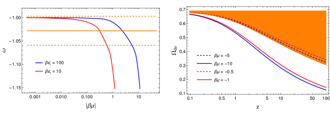
Figure 1: Left: Equation of state parameter (22) for different initial energies $\beta\epsilon_{i}$, as a function of $\beta\mu$. The orange lines represent the 68% C.L. constraints on the equation of state parameter for the $w$CDM model ($w=1.028\pm 0.031$ Aghanim:2018eyx ), using the combination of Planck, baryon acoustic oscillations (BAO) and SNe data. Right: Redshift evolution of the DE density parameter using the equation of state on the left plot, for the two corresponding choices $\beta\epsilon_{i}=100$ (blue) and $\beta\epsilon_{i}=10$ (red). The orange region represents the 68% C.L. constrains from Planck+BAO+SNe, for the phantom behavior.

IV Negative absolute temperature

The FDE model has an intrinsic cutoff to avoid a divergence in the energy and the minimum energy is the particle mass. These limits are similar to the ones in a scenario where a cosmological fluid possesses NAT, as investigated in Vieira:2016lyj .

The canonical absolute temperature can be defined as the variation of the entropy with the internal energy at thermal equilibrium

$$\frac{1}{T}=\left(\frac{\partial S}{\partial U}\right)_{V,N}\,,$$ (23)

which can be negative.

Necessary requirements for NAT are thermal equilibrium among the elements in the system and upper limit on the energy of the allowed states Ramsey:1956zz . Classically a system is not found with NAT because there is no upper bound on its energy. However, quantum mechanical systems can be constructed such that they possess an energy upper bound. In order scenarios this upper bound can be seen as an energy cutoff Vieira:2016lyj .

A system with NAT is hotter than the one with positive temperature because the former has more energy stored in it and can transfer its energy to any system at positive temperature it is in contact with purcell1951nuclear . Since a fluid with negative equation of state will have always an increasing temperature, it is natural to think that the NAT will be reached sometime in the evolution of this fluid.

In a cosmological context a fluid with positive temperature has the following number density, energy density and pressure Vieira:2016lyj

$$n(T,\mu) =\int_{m}^{\Lambda}D(\epsilon)\mathcal{N}(T,\epsilon,\mu)d\epsilon\,,$$ (24)

$$\rho(T,\mu) =\int_{m}^{\Lambda}\epsilon D(\epsilon)\mathcal{N}(T,\epsilon,\mu)d\epsilon\,,$$ (25)

$$P(T,\mu) =\beta^{-1}\int_{m}^{\Lambda}\epsilon D(\epsilon)\ln(1+e^{-\beta(\epsilon-\mu)})d\epsilon\,,$$ (26)

where $D(\epsilon)$ is the density of states and $\mathcal{N}(T,\epsilon,\mu)$ is the Fermi-Dirac distribution. The energy of the system is not bounded from above for bosons with no number conservation, therefore if $\mu=0$ a cosmological fluid with NAT can only be composed of fermions Vieira:2016lyj .

The symmetry of the Fermi-Dirac distribution and the logarithm in Eq. (26) allows the following relation between positive and negative temperatures

$$\mathcal{N}(T,\epsilon,\mu) =\frac{1}{e^{\beta(\epsilon-\mu)}+1}=1-\frac{1}{e^{-\beta(\epsilon-\mu)}+1}\,,$$

$$=1-\mathcal{N}(-T,\epsilon,\mu)\,,$$ (27)

$$\ln\big{[}1+e^{-\beta(\epsilon-\mu)}\big{]} =-\beta(\epsilon-\mu)+\ln\big{[}1+e^{\beta(\epsilon-\mu)}\big{]}\,.$$ (28)

As pointed out in Vieira:2016lyj , Eq. (27) indicates the idea of “holes” and “particles”, where holes are particles in the highest energy states (with $T<0$), which simply represent the absence of particles in states with positive temperature. The highest number density and energy density is thus when $\beta\rightarrow-\infty$, yielding

$$n_{\max} =\int_{m}^{\Lambda}D(\epsilon)d\epsilon=\frac{C^{-\frac{1}{w}}g}{6\pi^{2}}\big{(}m_{0}^{\frac{1}{w}}-\Lambda^{\frac{1}{w}}\big{)}\,,$$ (29)

$$\rho_{\max} =\int_{m}^{\Lambda}\epsilon D(\epsilon)d\epsilon\stackrel{{\scriptstyle w=-1}}{{=}}\frac{Cg}{6\pi^{2}}\big{[}\ln(\Lambda)-\ln(m_{0})\big{]}\,,$$ (30)

where the second equality in both equations comes from the fact that for FDE the density of states is $D(\epsilon)=-C^{-\frac{1}{w}}g/(6\pi^{2}w)\epsilon^{\frac{1}{w}-1}$. The lower limit of integration is $m=m_{0}$ because for negative temperatures $m=m_{0}+c_{0}|T|$ and $T=0^{-}$. From Eqs. (27) and (29) one can see that the maximum energy density and number density would be negative and thus unphysical, if bosons were considered instead of fermions.

Using the properties in Eqs. (27) and (28) one can obtain the following relations

$$n(T,\mu) =n_{\max}-n(-T,\mu)\,,$$ (31)

$$\rho(T,\mu) =\rho_{\max}-\rho(-T,\mu)\,,$$ (32)

$$P(T,\mu) =-\rho_{\max}+\mu n_{\max}-P(-T,\mu)\,.$$ (33)

In our case, both particles and holes (i.e., particles with $T>0$ or $T<0$) will be described by a fluid with the same negative equation of state parameter, since the corresponding density of states arises from the noncanonical kinetic term (6) in both regimes.

The number density and energy density for holes are still given by Eqs. (8) and (10) (or Eqs. (18) and (19) if $\mu\neq 0$), respectively, with the simple replacement $\beta\rightarrow|\beta|$ and the integrals are performed for negative $\beta$:

$$n_{h} =-\frac{C^{-\frac{1}{w}}g}{6\pi^{2}w}|\beta|^{-\frac{1}{w}}\mathscr{F}^{u_{\max},\,\beta\mu}_{u_{\min},\frac{1}{w}-1}\,,$$ (34)

$$\rho_{h} =-\frac{C^{-\frac{1}{w}}g}{6\pi^{2}w}|\beta|^{-\frac{1+w}{w}}\mathscr{F}^{u_{\max},\,\beta\mu}_{u_{\min},\frac{1}{w}}\,,$$ (35)

where here $u\equiv-|\beta|(\epsilon-\mu)$ and the subscripts “p” and “h” will indicate particles with $T>0$ and with $T<0$, respectively. Contrary to the case of positive $T$ ($\infty<\beta<0^{+}$), the negative temperature makes the number density to grow with $|\beta|$, because an increase in a negative temperature corresponds to an increase in $|\beta|$. The following relations also hold

$$\rho_{h}=|\beta|^{-1}\frac{\mathscr{F}^{u_{\max},\,\beta\mu}_{u_{\min},\frac{1}{w}}}{\mathscr{F}^{u_{\max},\,\beta\mu}_{u_{\min},\frac{1}{w}-1}}n_{h}\,.$$ (36)

$$\frac{\dot{T}}{T}=-\frac{\dot{\beta}}{\beta}=\frac{\partial P}{\partial\rho}\frac{\dot{n}_{p,h}}{n_{p,h}}\,.$$ (37)

Eq. (37) also yields $n_{p}\propto\beta^{-\frac{1}{w}}$ and $n_{h}\propto|\beta|^{-\frac{1}{w}}$, thus the number density of holes increases up to $n_{\max}$.

The number conservation equation and the continuity equation for particles and holes are

$$\dot{n}_{p}+3Hn_{p} =0\,,$$ (38)

$$\dot{n}_{h}+3H(n_{h}-n_{\max}) =0\,,$$ (39)

$$\dot{\rho}_{p}+3H(1+w)\rho_{p} =0\,,$$ (40)

$$\dot{\rho}_{h}+3H(1+w)\rho_{h} =0\,.$$ (41)

The solution of Eq. (39) is $n_{h}=n_{\max}-n_{\max}(a_{*}/a)^{3}$, where the scale factor $a_{*}$ represents the time when the initial abundance of particles was equal to the maximum number density $n_{p}^{*}=n_{\max}$. This solution means that in the early Universe all states with positive temperature were filled and $n_{h}=0$. As the Universe evolves $n_{p}$ decreases and $n_{h}$ increases up to $n_{\max}$. When $\beta\rightarrow 0$ both number densities are equal to half of the maximum number density, $n_{p}=n_{h}=n_{\max}$/2. Since $n_{h}\propto|\beta|$ NAT increase as $|\beta|\propto n_{\max}(1-(a_{*}/a)^{3})$, while for positive temperatures the scaling is linear $T=\beta^{-1}\propto V$.

The number conservation was required in Vieira:2016lyj because for canonical particles the number conservation equation and the continuity equation gave inconsistent results. For example, for nonrelativistic particles ($w=0$) Eq. (39) can be multiplied by $m$, but it does not yield Eq. (41). However, this problem is solved for FDE. Taking the time derivative of Eqs. (21) and (36), for particles and holes, respectively, and using Eqs. (37), (38) and (39), we obtain

$$\dot{\rho}_{p} =-3H(1+w)\rho_{p}\,,$$ (42)

$$\dot{\rho}_{h} =-3H(1+w)\rho_{h}+3H(1+w)\rho_{h}\frac{n_{\max}}{n_{h}}\,.$$ (43)

Eq. (43) is equal to Eq. (41) if $w\approx-1$. Hence, in this scenario the chemical potential should be approximately zero.

Eqs. (8) and (34) do not include the case when $\beta\rightarrow 0$. In this limit both particles and holes are equally distributed , so that $n_{p}=n_{h}=n_{\max}/2$. The full results are then

$$n_{p} =\frac{Cg}{6\pi^{2}}\beta\mathscr{F}^{u_{\max},\,+\beta}_{u_{\min},-2}+\frac{n_{\max}}{2}\,,$$ (44)

$$n_{h} =\frac{Cg}{6\pi^{2}}|\beta|\mathscr{F}^{u_{\max},\,-\beta}_{u_{\min},-2}+\frac{n_{\max}}{2}\,,$$ (45)

where the subscripts $\pm\beta$ in $\mathscr{F}^{u_{\max}}_{u_{\min},-2}$ are simply to indicate the regime in which the integrals are referred to.

Using Eqs. (44) and (45) we plot in Fig. 2 the ratios $n_{p}/n_{\max}=\beta m_{0}\mathscr{F}^{u_{\max},\,+\beta}_{u_{\min},-2}+1/2$ and $n_{h}/n_{\max}=|\beta|m_{0}\mathscr{F}^{u_{\max},\,-\beta}_{u_{\min},-2}+1/2$ with $u_{\min}=3$, as a function of $\beta m_{0}$. The maximum combination $\beta m_{0}$ for positive temperature that gives $n_{p}=n_{\max}$ is $\beta m_{0}=145$, while $n_{h}=n_{\max}$ for $\beta m_{0}=-1.5$. Soon after the FDE particles reach the transition $+T\rightarrow-T$, they quickly reach the maximum negative temperature $T=0^{-}$. This behavior happens because both energy and temperature increase with the volume, then when the energy of the particles reach the cutoff the volume continue increasing and $\epsilon/T$ is no longer constant, enabling a transition from positive to negative temperatures $\beta\Lambda\ll 1$. However, once the particles reach the cutoff, they populate the highest energy state, and the number density and energy density of the system are at their corresponding maximum values. Therefore, the transition $+\infty\rightarrow-T\rightarrow 0^{-}$ happens in a very short time interval. Different values of $u_{\min}$ lead to similar behavior. If $u_{\min}=10$, then $n_{p}=n_{\max}$ for $\beta m_{0}=10^{6}$, and $n_{h}=n_{\max}$ for $\beta m_{0}=-5$. The maximum $+\beta$ for a given mass is the minimum possible temperature at the transition of canonical nonrelativistic matter to noncanonical nonrelativisitic matter, i.e., when the noncanonical kinetic term dominates and the temperature of the system stops decreasing to start increasing.

Since positive temperatures scale with the volume, a variation from $\beta m_{0}$ to zero corresponds to a decrease of $\beta m_{0}(z_{\beta=0}+1)^{3}/(z_{*}+1)^{3}$, where the redshift $z_{*}$ corresponds when $n_{p}=n_{\max}$, that is, at the beginning of the FDE evolution. If $\beta m_{0}=10^{6}$ and the redshift of FDE formation is $z_{*}=10^{12}$, at redshift $10^{8}$ the combination $\beta m_{0}$ is reduced to $10^{-6}$. A similar reduction happens for $z_{*}=10^{9}$ and $z_{\beta=0}=10^{5}$. For the smaller value $\beta m_{0}=145$ the transition from positive to negative temperatures happens much faster.

The fact that $n_{h}\approx n_{\max}\gg n_{p}$, soon after the temperature becomes negative, indicates from the number conservation equation that $\dot{n}_{h}=0$, thus the holes are not diluted as the Universe expands, but fill all the high-energy states. The behavior of FDE particles therefore does not suffer from the problems presented in Vieira:2016lyj when the number of particles is conserved.

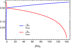
Figure 2: Ratio between the particle (hole) number density to the maximum number density in blue (red), as a function of $\beta m_{0}$. The temperature increases from right to left.

For positive $\beta$ we have, for example, $\mathscr{F}^{10^{4}}_{10,-1}=10^{-6}$ while $\mathscr{F}^{10^{4}}_{10,-1}=7$ for negative $\beta$. If $u_{\min}$ is one order of magnitude smaller, then $\mathscr{F}^{10^{4}}_{3,-1}=10^{-2}$ for positive $\beta$ and $\mathscr{F}^{10^{4}}_{3,-1}=8$ for negative $\beta$. These results indicate that the constant $C$ should be of order $10^{-46}$ GeV⁴, i.e., $C=\lambda^{6}M_{Pl}^{-2}$, with $\lambda\sim 10^{-8/6}$ GeV, to give the observed value of the vacuum energy. Since the maximum energy density depends logarithmically on the cutoff scale, even arbitrarily large values of $\Lambda\sim 10^{19}$ GeV would still give the observed value of the vacuum energy if the constant is $C\sim 10^{-47}$ GeV⁴. Using the parametrization including the Planck mass, the length scale is $(M_{Pl}^{2}/\lambda^{6})^{1/4}$, indicating that the length $\lambda^{-1}$ is of order $10^{7.8}l_{p}^{1/3}\sim 10^{3/2}$ GeV^-1, where $l_{p}$ is the Planck length.

The energy density is constant for both particles and holes, and we can see its evolution and the transition from $+T$ to $-T$ in Fig. 3, where we selected the corresponding initial energy $\beta\epsilon_{i}=3$, which is the minimum allowed value for this parameter. Other choices for the minimum energy would give very similar results. Since the equation of state should be minus one, DE perturbations are practically zero.

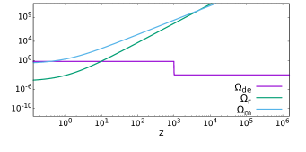
Figure 3: Evolution of the density parameter for radiation, matter and dark energy with a illustrative transition from $+T$ to $-T$ at redshift $10^{3}$.

In order to investigate the impact of this transition in the early Universe, we will use cosmological observations to constrain the redshift of the transition $z_{\beta=0}$ and the usual six $\Lambda$CDM parameters. We take the same initial energy as before and use an adapted version of CLASS blas2011cosmic , along with MontePython Audren:2012wb ; Brinckmann:2018cvx to constrain the cosmological parameters.

We use different set of observations from the following surveys: CMB anisotropy results from Planck high-$\ell$ and low-$\ell$ temperature and polarization power spectra (TT, TE, EE) Planck:2019nip and lensing measurements Planck:2018lbu ; BAO measurements from 6dFGS beutler20116df , MGS Ross:2014qpa , BOSS DR12 BOSS:2016wmc , and the auto and cross-correlation of Ly$\alpha$ absorption and quasars in eBOSS DR14 Blomqvist:2019rah ; deSainteAgathe:2019voe ; and 1048 SNe from the Pantheon sample Scolnic:2017caz . We constrain the nuisance parameters along with the cosmological ones and we use the Gelman-Rubin criterion gelman1992inference $R-1<0.06$ to assume that the chains converged. We use a prior on the redshift $z_{\beta=0}$ [1, $10^{10}$] so that DE dominates at very late times.

We show in Fig. 4 the constraints on the redshift of the transition from $+T$ to $-T$ and the other six parameters for the joint analysis of CMB + BAO and CMB + BAO + SNe. We present in Table 1 the best fit and 68% C.L. values for all parameters. The results are consistent with the $\Lambda$CDM model and the transition from positive to negative temperatures could have happened at any redshift $z_{\beta=0}>1$, thus in agreement with the cosmological observations. This agreement reflects the fact that the energy density for DE is much smaller than the corresponding ones for matter and radiation, at higher redshifts.

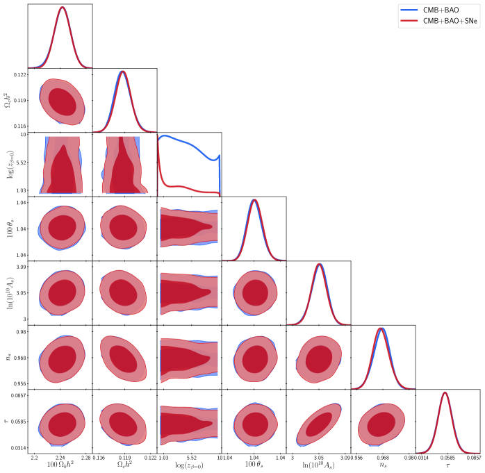
Figure 4: 1D and 2D (68% and 95% C.L.) posterior distributions of the cosmological parameters for the combinations CMB + BAO and CMB + BAO + SNe.

Table 1: Cosmological parameters using CMB, BAO and SNe data.

Parameter	CMB + BAO		CMB + BAO + SNe
	Best fit	68% limits	Best fit	68% limits
$100\,\Omega{}_{b}h^{2}$	$2.246$	$2.244_{-0.014}^{+0.015}$	$2.243$	$2.244_{-0.015}^{+0.014}$
$\Omega{}_{c}h^{2}$	$0.1189$	$0.119_{-0.001}^{+0.001}$	$0.1189$	$0.119_{-0.001}^{+0.001}$
$100\,\theta{}_{s}$	$1.0421$	$1.0420_{-0.0003}^{+0.0003}$	$1.0419$	$1.0420_{-0.0003}^{+0.0003}$
$\ln(10^{10}A_{{s}})$	$3.046$	$3.045_{-0.015}^{+0.015}$	$3.034$	$3.045_{-0.015}^{+0.015}$
$n_{s}$	$0.9669$	$0.9674_{-0.0040}^{+0.0042}$	$0.9658$	$0.9672_{-0.0040}^{+0.0040}$
$\tau$	$0.0541$	$0.0553_{-0.0075}^{+0.0078}$	$0.0509$	$0.0556_{-0.0079}^{+0.0077}$
$\log(z_{\beta=0})$	$4.48$	$4.63_{-4.44}^{+1.54}$	$3.64$	$3.80_{-3.54}^{+1.13}$
$H_{0}$	$67.93$	$67.86_{-0.57}^{+0.49}$	$67.83$	$68.00_{-0.68}^{+0.37}$
$\Omega{}_{m}$	$0.3078$	$0.3090_{-0.0061}^{+0.0066}$	$0.3086$	$0.3079_{-0.0053}^{+0.0069}$
$\chi^{2}_{\min}$	$2790$		$3817$

V Conclusions

In this paper we have investigated further aspects of the FDE model. First, we analyzed FDE with a nonzero chemical potential. In this case, FDE possesses a phantom behavior and the equation of state parameter has a lower limit. The combination of temperature and chemical potential $\beta\mu$ is constrained by measurements of $w$ by Planck, giving an upper bound of $\beta\mu\lesssim 5\%\beta\epsilon$.

In the second part of this paper we analyzed the NAT behavior for FDE. In order to avoid a divergence in the energy when the momentum goes to zero, a cutoff is introduced. This cutoff is precisely a requirement for NAT, thus indicating a connection between FDE and NAT, if FDE is composed of fermions. In this case the equation of state parameter should be equal to minus one and the chemical potential should be zero. We have shown that when the energy of the system reaches the cutoff, the transition to NAT happens and in fact, all high-energy states become quickly populated, leading in turn to the maximum energy density and number density for the system. Negative temperatures saturates ($T=0^{-}$) in a very short time and the holes are no longer diluted as the Universe expands. Using combined data from CMB, BAO and SNe, we investigated the redshift of the transition from $+T$ to $-T$ and the results indicated that this transition is allowed at any redshift larger than one. This connection between FDE and NAT elucidates the properties of the present model and shows a possible fate of the FDE gas.

- [1] S. Perlmutter et al. Measurements of Omega and Lambda from 42 high redshift supernovae. Astrophys. J., 517:565–586, 1999.
- [2] A. G. Riess et al. Observational evidence from supernovae for an accelerating universe and a cosmological constant. Astron. J., 116:1009–1038, 1998.
- [3] N. Aghanim et al. Planck 2018 results. VI. Cosmological parameters. Astron. Astrophys., 641:A6, 2020.
- [4] Adam G. Riess, Stefano Casertano, Wenlong Yuan, J. Bradley Bowers, Lucas Macri, Joel C. Zinn, and Dan Scolnic. Cosmic Distances Calibrated to 1% Precision with Gaia EDR3 Parallaxes and Hubble Space Telescope Photometry of 75 Milky Way Cepheids Confirm Tension with CDM. Astrophys. J. Lett., 908(1):L6, 2021.
- [5] P. J. E. Peebles and B. Ratra. Cosmology with a Time Variable Cosmological Constant. Astrophys. J., 325:L17, 1988.
- [6] B. Ratra and P. J. E. Peebles. Cosmological Consequences of a Rolling Homogeneous Scalar Field. Phys. Rev., D37:3406, 1988.
- [7] J. A. Frieman, C. T. Hill, and R. Watkins. Late time cosmological phase transitions. 1. Particle physics models and cosmic evolution. Phys. Rev., D46:1226–1238, 1992.
- [8] J. A. Frieman, C. T. Hill, A. Stebbins, and I. Waga. Cosmology with ultralight pseudo Nambu-Goldstone bosons. Phys. Rev. Lett., 75:2077, 1995.
- [9] R. R. Caldwell, R. Dave, and P. J. Steinhardt. Cosmological imprint of an energy component with general equation of state. Phys. Rev. Lett., 80:1582, 1998.
- [10] T. Padmanabhan. Accelerated expansion of the universe driven by tachyonic matter. Phys. Rev., D66:021301, 2002.
- [11] J. S. Bagla, H. K. Jassal, and T. Padmanabhan. Cosmology with tachyon field as dark energy. Phys. Rev., D67:063504, 2003.
- [12] C. Armendariz-Picon, V. F. Mukhanov, and P. J. Steinhardt. A Dynamical solution to the problem of a small cosmological constant and late time cosmic acceleration. Phys. Rev. Lett., 85:4438–4441, 2000.
- [13] P. Brax and J. Martin. Quintessence and supergravity. Phys. Lett., B468:40–45, 1999.
- [14] E. J. Copeland, N. J. Nunes, and F. Rosati. Quintessence models in supergravity. Phys. Rev., D62:123503, 2000.
- [15] S. Vagnozzi, S. Dhawan, M. Gerbino, K. Freese, A. Goobar, and O. Mena. Constraints on the sum of the neutrino masses in dynamical dark energy models with are tighter than those obtained in CDM. Phys. Rev., D98(8):083501, 2018.
- [16] T. Koivisto and D. F. Mota. Vector Field Models of Inflation and Dark Energy. JCAP, 0808:021, 2008.
- [17] K. Bamba and S. D. Odintsov. Inflation and late-time cosmic acceleration in non-minimal Maxwell- gravity and the generation of large-scale magnetic fields. JCAP, 0804:024, 2008.
- [18] V. Emelyanov and F. R. Klinkhamer. Possible solution to the main cosmological constant problem. Phys. Rev., D85:103508, 2012.
- [19] V. Emelyanov and F. R. Klinkhamer. Reconsidering a higher-spin-field solution to the main cosmological constant problem. Phys. Rev., D85:063522, 2012.
- [20] V. Emelyanov and F. R. Klinkhamer. Vector-field model with compensated cosmological constant and radiation-dominated FRW phase. Int. J. Mod. Phys., D21:1250025, 2012.
- [21] S. Kouwn, P. Oh, and C.-G. Park. Massive Photon and Dark Energy. Phys. Rev., D93(8):083012, 2016.
- [22] R. C. G. Landim. Cosmological tracking solution and the Super-Higgs mechanism. Eur. Phys. J., C76(8):430, 2016.
- [23] R. C. G. Landim. Dynamical analysis for a vector-like dark energy. Eur. Phys. J., C76:480, 2016.
- [24] Aritra Banerjee, Haiying Cai, Lavinia Heisenberg, Eoin Ó. Colgáin, M. M. Sheikh-Jabbari, and Tao Yang. Hubble sinks in the low-redshift swampland. Phys. Rev. D, 103(8):L081305, 2021.
- [25] M.k Szydlowski, A. Stachowski, and K. Urbanowski. Quantum mechanical look at the radioactive-like decay of metastable dark energy. Eur. Phys. J., C77(12):902, 2017.
- [26] A. Stachowski, M. Szydlowski, and . Urbanowski. Cosmological implications of the transition from the false vacuum to the true vacuum state. Eur. Phys. J., C77(6):357, 2017.
- [27] D. Stojkovic, G. D. Starkman, and R. Matsuo. Dark energy, the colored anti-de Sitter vacuum, and LHC phenomenology. Phys. Rev., D77:063006, 2008.
- [28] E. Greenwood, E. Halstead, R. Poltis, and D. Stojkovic. Dark energy, the electroweak vacua and collider phenomenology. Phys. Rev., D79:103003, 2009.
- [29] E. Abdalla, L. L. Graef, and B. Wang. A Model for Dark Energy decay. Phys. Lett., B726:786–790, 2013.
- [30] A. Shafieloo, D. K. Hazra, V. Sahni, and A. A. Starobinsky. Metastable Dark Energy with Radioactive-like Decay. Mon. Not. Roy. Astron. Soc., 473:2760–2770, 2018.
- [31] R. G. Landim and E. Abdalla. Metastable dark energy. Phys. Lett. B., 764:271, 2017.
- [32] Ricardo G. Landim. Dark energy, scalar singlet dark matter and the Higgs portal. Mod. Phys. Lett., A33(15):1850087, 2018.
- [33] Ricardo G. Landim, Rafael J. F. Marcondes, Fabrízio F. Bernardi, and Elcio Abdalla. Interacting Dark Energy in the Dark Model. Braz. J. Phys., 48(4):364–369, 2018.
- [34] S. D. H. Hsu. Entropy bounds and dark energy. Phys. Lett., B594:13–16, 2004.
- [35] M. Li. A model of holographic dark energy. Phys. Lett., B603:1, 2004.
- [36] D. Pavon and W. Zimdahl. Holographic dark energy and cosmic coincidence. Phys. Lett., B628:206–210, 2005.
- [37] B. Wang, Y.-G. Gong, and E. Abdalla. Transition of the dark energy equation of state in an interacting holographic dark energy model. Phys. Lett., B624:141–146, 2005.
- [38] B. Wang, Y. Gong, and E. Abdalla. Thermodynamics of an accelerated expanding universe. Phys. Rev., D74:083520, 2006.
- [39] B. Wang, C.-Y. Lin, and E. Abdalla. Constraints on the interacting holographic dark energy model. Phys. Lett., B637:357–361, 2006.
- [40] B. Wang, C.-Y. Lin, D. Pavon, and E. Abdalla. Thermodynamical description of the interaction between dark energy and dark matter. Phys. Lett., B662:1–6, 2008.
- [41] R. C. G. Landim. Holographic dark energy from minimal supergravity. Int. J. Mod. Phys., D25(4):1650050, 2016.
- [42] M. Li, X.-D. Li, S. Wang, and X. Zhang. Holographic dark energy models: A comparison from the latest observational data. JCAP, 0906:036, 2009.
- [43] M. Li, X.-D. Li, S. Wang, Y. Wang, and X. Zhang. Probing interaction and spatial curvature in the holographic dark energy model. JCAP, 0912:014, 2009.
- [44] M. Li, X.-D. Li, S. Wang, and Y. Wang. Dark Energy. Commun. Theor. Phys., 56:525–604, 2011.
- [45] Emmanuel N. Saridakis. Ricci-Gauss-Bonnet holographic dark energy. Phys. Rev. D, 97(6):064035, 2018.
- [46] A. Al Mamon. Reconstruction of interaction rate in holographic dark energy model with Hubble horizon as the infrared cut-off. Int. J. Mod. Phys., D26(11):1750136, 2017.
- [47] A. Mukherjee. Reconstruction of interaction rate in Holographic dark energy. JCAP, 1611:055, 2016.
- [48] L. Feng and X. Zhang. Revisit of the interacting holographic dark energy model after Planck 2015. JCAP, 1608(08):072, 2016.
- [49] R. Herrera, W. S. Hipolito-Ricaldi, and N. Videla. Instability in interacting dark sector: An appropriate Holographic Ricci dark energy model. JCAP, 1608:065, 2016.
- [50] M. Forte. Holographik, the k-essential approach to interactive models with modified holographic Ricci dark energy. Eur. Phys. J., C76(12):707, 2016.
- [51] C. Wetterich. The Cosmon model for an asymptotically vanishing time dependent cosmological ’constant’. Astron. Astrophys., 301:321–328, 1995.
- [52] L. Amendola. Coupled quintessence. Phys. Rev., D62:043511, 2000.
- [53] Z.-K. Guo and Y.-Z. Zhang. Interacting phantom energy. Phys. Rev. D., 71:023501, 2005.
- [54] R.-G. Cai and A. Wang. Cosmology with interaction between phantom dark energy and dark matter and the coincidence problem. JCAP, 0503:002, 2005.
- [55] Z.-K. Guo, R.-G. Cai, and Y.-Z. Zhang. Cosmological evolution of interacting phantom energy with dark matter. JCAP, 0505:002, 2005.
- [56] X.-J. Bi, B. Feng, H. Li, and X. Zhang. Cosmological evolution of interacting dark energy models with mass varying neutrinos. Phys. Rev. D., 72:123523, 2005.
- [57] B. Gumjudpai, T. Naskar, M. Sami, and S. Tsujikawa. Coupled dark energy: Towards a general description of the dynamics. JCAP, 0506:007, 2005.
- [58] Shaoyu Yin, Bin Wang, Elcio Abdalla, and Chi-Yong Lin. The Transition of equation of state of effective dark energy in the DGP model with bulk contents. Phys. Rev. D, 76:124026, 2007.
- [59] A. A. Costa, X.-D. Xu, B. Wang, E. G. M. Ferreira, and E. Abdalla. Testing the Interaction between Dark Energy and Dark Matter with Planck Data. Phys. Rev., D89(10):103531, 2014.
- [60] E. G. M. Ferreira, J. Quintin, A. A. Costa, E. Abdalla, and B. Wang. Evidence for interacting dark energy from BOSS. Phys. Rev., D95(4):043520, 2017.
- [61] A. A. Costa, L. C. Olivari, and E. Abdalla. Quintessence with Yukawa Interaction. Phys. Rev., D92(10):103501, 2015.
- [62] R. C. G. Landim. Coupled tachyonic dark energy: a dynamical analysis. Int. J. Mod. Phys., D24:1550085, 2015.
- [63] R. C. G. Landim. Coupled dark energy: a dynamical analysis with complex scalar field. Eur. Phys. J., C76(1):31, 2016.
- [64] A. A. Costa, X.-D. Xu, B. Wang, and E. Abdalla. Constraints on interacting dark energy models from Planck 2015 and redshift-space distortion data. JCAP, 1701(01):028, 2017.
- [65] R. J. F. Marcondes, R. C. G. Landim, A. A. Costa, B. Wang, and E. Abdalla. Analytic study of the effect of dark energy-dark matter interaction on the growth of structures. JCAP, 1612(12):009, 2016.
- [66] F. F. Bernardi and R. G. Landim. Coupled quintessence and the impossibility of an interaction: a dynamical analysis study. Eur. Phys. J., C77(5):290, 2017.
- [67] B. Wang, E. Abdalla, F. Atrio-Barandela, and D. Pavon. Dark Matter and Dark Energy Interactions: Theoretical Challenges, Cosmological Implications and Observational Signatures. Rep. Prog. Phys., 79(9):096901, 2016.
- [68] G. R. Farrar and P. J. E. Peebles. Interacting dark matter and dark energy. Astrophys. J., 604:1–11, 2004.
- [69] S. Micheletti, E. Abdalla, and B. Wang. A Field Theory Model for Dark Matter and Dark Energy in Interaction. Phys. Rev., D79:123506, 2009.
- [70] W. Yang, N. Banerjee, and S. Pan. Constraining a dark matter and dark energy interaction scenario with a dynamical equation of state. Phys. Rev., D95(12):123527, 2017.
- [71] R. F. vom Marttens, L. Casarini, W. S. Hipólito-Ricaldi, and W. Zimdahl. CMB and matter power spectra with non-linear dark-sector interactions. JCAP, 1701(01):050, 2017.
- [72] Weiqiang Yang, Supriya Pan, and John D. Barrow. Large-scale Stability and Astronomical Constraints for Coupled Dark-Energy Models. Phys. Rev., D97(4):043529, 2018.
- [73] Andre A. Costa, Ricardo C.G. Landim, Bin Wang, and E. Abdalla. Interacting Dark Energy: Possible Explanation for 21-cm Absorption at Cosmic Dawn. Eur. Phys. J. C, 78(9):746, 2018.
- [74] W. Yang, S. Pan, E. Di Valentino, R. C. Nunes, S. Vagnozzi, and D. F. Mota. Tale of stable interacting dark energy, observational signatures, and the tension. JCAP, 1809(09):019, 2018.
- [75] Ricardo G. Landim. Cosmological perturbations and dynamical analysis for interacting quintessence. Eur. Phys. J. C, 79(11):889, 2019.
- [76] Sunny Vagnozzi, Luca Visinelli, Olga Mena, and David F. Mota. Do we have any hope of detecting scattering between dark energy and baryons through cosmology? Mon. Not. Roy. Astron. Soc., 493(1):1139–1152, 2020.
- [77] G. Dvali, G. Gabadadze, and M. Porrati. 4D Gravity on a Brane in 5D Minkowski Space. Phys. Lett. B, 485:208, 2000.
- [78] Ricardo G. Landim. Fractional dark energy. Phys. Rev. D, 103(8):083511, 2021.
- [79] Nick Laskin. Fractional quantum mechanics. World Scientific, 2018.
- [80] Nick Laskin. Fractional quantum mechanics. Phys. Rev. E, 62(3):3135, 2000.
- [81] Nick Laskin. Fractional Schrodinger equation. Phys. Rev. E, 66:056108, 2002.
- [82] Xiaoyi Guo and Mingyu Xu. Some physical applications of fractional schrödinger equation. J. Math. Phys., 47(8):082104, 2006.
- [83] Selçuk Ş Bayın. On the consistency of the solutions of the space fractional schrödinger equation. J. Math. Phys., 53(4):042105, 2012.
- [84] Selçuk Ş Bayın. Comment on “on the consistency of the solutions of the space fractional schrödinger equation”[j. math. phys. 53, 042105 (2012)]. J. of Math. Phys., 53(8):084101, 2012.
- [85] Jianping Dong and Mingyu Xu. Some solutions to the space fractional schrödinger equation using momentum representation method. J. Math. Phys., 48(7):072105, 2007.
- [86] Edmundo Capelas de Oliveira, Felix Silva Costa, and Jayme Vaz Jr. The fractional schrödinger equation for delta potentials. J. Math. Phys., 51(12):123517, 2010.
- [87] Andrea Giusti, Roberto Garrappa, and Geneviève Vachon. On the Kuzmin model in fractional Newtonian gravity. Eur. Phys. J. Plus, 135(10):798, 2020.
- [88] Andrea Giusti. MOND-like Fractional Laplacian Theory. Phys. Rev. D, 101(12):124029, 2020.
- [89] P.V. Moniz and S. Jalalzadeh. From Fractional Quantum Mechanics to Quantum Cosmology: An Overture. Mathematics, 8(3):313, 2020.
- [90] S. M. M. Rasouli, S. Jalalzadeh, and P. V. Moniz. Broadening quantum cosmology with a fractional whirl. Mod. Phys. Lett. A, 36(14):2140005, 2021.
- [91] Edward M Purcell and Robert V Pound. A nuclear spin system at negative temperature. Physical Review, 81(2):279, 1951.
- [92] Lars Onsager. Statistical hydrodynamics. Il Nuovo Cimento (1943-1954), 6(2):279–287, 1949.
- [93] Norman F. Ramsey. Thermodynamics and Statistical Mechanics at Negative Absolute Temperatures. Phys. Rev., 103:20–28, 1956.
- [94] Martin J Klein. Negative absolute temperatures. Physical Review, 104(3):589, 1956.
- [95] Simon Braun, Jens Philipp Ronzheimer, Michael Schreiber, Sean S Hodgman, Tim Rom, Immanuel Bloch, and Ulrich Schneider. Negative absolute temperature for motional degrees of freedom. Science, 339(6115):52–55, 2013.
- [96] AS Oja and OV Lounasmaa. Nuclear magnetic ordering in simple metals at positive and negative nanokelvin temperatures. Reviews of Modern Physics, 69(1):1, 1997.
- [97] Patrick Medley, David M Weld, Hirokazu Miyake, David E Pritchard, and Wolfgang Ketterle. Spin gradient demagnetization cooling of ultracold atoms. Physical review letters, 106(19):195301, 2011.
- [98] J. P. P. Vieira, Christian T. Byrnes, and Antony Lewis. Cosmology with Negative Absolute Temperatures. JCAP, 08:060, 2016.
- [99] Keith Oldham and Jerome Spanier. The fractional calculus theory and applications of differentiation and integration to arbitrary order. Dover, 2006.
- [100] Gianluca Calcagni. Multifractional theories: an updated review. Mod. Phys. Lett. A, 36(14):2140006, 2021.
- [101] Gianluca Calcagni. Quantum scalar field theories with fractional operators. Class. Quant. Grav., 38(16):165006, 2021.
- [102] Gianluca Calcagni. Classical and quantum gravity with fractional operators. Class. Quant. Grav., 38(16):165005, 2021. [Erratum: Class.Quant.Grav. 38, 169601 (2021)].
- [103] Steven Weinberg. Entropy generation and the survival of protogalaxies in an expanding universe. Astrophys. J., 168:175, 1971.
- [104] R. Silva, J.A.S. Lima, and M.O. Calvao. Temperature evolution law of imperfect relativistic fluids. Gen. Rel. Grav., 34:865–875, 2002.
- [105] Herbert B Callen. Thermodynamics and an Introduction to Thermostatistics. American Association of Physics Teachers, 1998.
- [106] J. A. S. Lima and S. H. Pereira. Chemical Potential and the Nature of the Dark Energy: The case of phantom. Phys. Rev. D, 78:083504, 2008.
- [107] Diego Blas, Julien Lesgourgues, and Thomas Tram. The cosmic linear anisotropy solving system (class). part ii: approximation schemes. Journal of Cosmology and Astroparticle Physics, 2011(07):034, 2011.
- [108] Benjamin Audren, Julien Lesgourgues, Karim Benabed, and Simon Prunet. Conservative Constraints on Early Cosmology: an illustration of the Monte Python cosmological parameter inference code. JCAP, 1302:001, 2013.
- [109] Thejs Brinckmann and Julien Lesgourgues. MontePython 3: boosted MCMC sampler and other features. Phys. Dark Univ., 24:100260, 2019.
- [110] N. Aghanim et al. Planck 2018 results. V. CMB power spectra and likelihoods. Astron. Astrophys., 641:A5, 2020.
- [111] N. Aghanim et al. Planck 2018 results. VIII. Gravitational lensing. Astron. Astrophys., 641:A8, 2020.
- [112] Florian Beutler, Chris Blake, Matthew Colless, D Heath Jones, Lister Staveley-Smith, Lachlan Campbell, Quentin Parker, Will Saunders, and Fred Watson. The 6df galaxy survey: baryon acoustic oscillations and the local hubble constant. Monthly Notices of the Royal Astronomical Society, 416(4):3017–3032, 2011.
- [113] Ashley J. Ross, Lado Samushia, Cullan Howlett, Will J. Percival, Angela Burden, and Marc Manera. The clustering of the SDSS DR7 main Galaxy sample – I. A 4 per cent distance measure at . Mon. Not. Roy. Astron. Soc., 449(1):835–847, 2015.
- [114] Shadab Alam et al. The clustering of galaxies in the completed SDSS-III Baryon Oscillation Spectroscopic Survey: cosmological analysis of the DR12 galaxy sample. Mon. Not. Roy. Astron. Soc., 470(3):2617–2652, 2017.
- [115] Michael Blomqvist et al. Baryon acoustic oscillations from the cross-correlation of Ly absorption and quasars in eBOSS DR14. Astron. Astrophys., 629:A86, 2019.
- [116] Victoria de Sainte Agathe et al. Baryon acoustic oscillations at z = 2.34 from the correlations of Ly absorption in eBOSS DR14. Astron. Astrophys., 629:A85, 2019.
- [117] D. M. Scolnic et al. The Complete Light-curve Sample of Spectroscopically Confirmed SNe Ia from Pan-STARRS1 and Cosmological Constraints from the Combined Pantheon Sample. Astrophys. J., 859(2):101, 2018.
- [118] Andrew Gelman and Donald B Rubin. Inference from iterative simulation using multiple sequences. Statistical science, 7(4):457–472, 1992.