Vacuum correlators at short distances from lattice QCD

Abstract

Non-perturbatively computing the hadronic vacuum polarization at large photon virtualities and making contact with perturbation theory enables a precision determination of the electromagnetic coupling at the $Z$ pole, which enters global electroweak fits. In order to achieve this goal ab initio using lattice QCD, one faces the challenge that, at the short distances which dominate the observable, discretization errors are hard to control. Here we address challenges of this type with the help of static screening correlators in the high-temperature phase of QCD, yet without incurring any bias. The idea is motivated by the observations that (a) the cost of high-temperature simulations is typically much lower than their vacuum counterpart, and (b) at distances $x_{3}$ far below the inverse temperature $1/T$, the operator-product expansion guarantees the thermal correlator of two local currents to deviate from the vacuum correlator by a relative amount that is power-suppressed in $(x_{3}\>T)$. The method is first investigated in lattice perturbation theory, where we point out the appearance of an O$(a^{2}\log(1/a))$ lattice artifact in the vacuum polarization with a prefactor that we calculate. It is then applied to non-perturbative lattice QCD data with two dynamical flavors of quarks. Our lattice spacings range down to 0.049 fm for the vacuum simulations and down to 0.033 fm for the simulations performed at a temperature of 250 MeV.

I Introduction

Many phenomenologically interesting observables are defined in terms of QCD vacuum correlators involving two or more local fields integrated over their Euclidean positions. For example, the hadronic vacuum polarization function $\widehat{\Pi}(Q^{2})$, which determines the leading hadronic contribution to the running of the electromagnetic coupling and the muon anomalous magnetic moment $(g-2)_{\mu}$, the $\pi^{0}\to\gamma^{*}\gamma^{*}$ transition form factor of the pion and the hadronic light-by-light contribution to $(g-2)_{\mu}$ are expressed in such a way. Thus in many cases, vacuum correlators represent crucial input for precision tests of the Standard Model. Lattice QCD provides ab initio determinations of these vacuum correlators; see e.g. Refs. Burger et al. (2015); Francis et al. (2015); Gérardin et al. (2019); Aoyama et al. (2020) for the applications above.

However, these integrated quantities contain contributions corresponding to the fields being close together, a regime which can lead to large cutoff effects. The standard tool to investigate the asymptotic approach to the continuum limit of correlation functions is Symanzik’s effective field theory Symanzik (1983); Lüscher (1998); Weisz (2010). A complication for the aforementioned observables is that the on-shell improvement programme is not sufficient to guarantee rapid convergence toward the continuum limit. In this work, we propose to compute the short-distance contribution to vacuum correlators by making use of static screening correlators from QCD at finite temperature, which can significantly reduce the cost of obtaining a robust continuum limit. As the short-distance contribution has little sensitivity to the temperature, the bulk of this contribution can be computed using particularly small lattice spacings in the high-temperature phase of QCD, where the cost of the simulations is much reduced, and only a small remainder needs to be computed using the vacuum ensembles. Just as importantly, the cutoff effects on the remainder can be arranged to be parametrically smaller than those of the observable computed on thermal gauge ensembles. Furthermore, we note that in certain cases, there is a logarithmic enhancement of the cutoff effects on the short-distance contribution at leading order in perturbation theory, in contrast to the modification of cutoff effects by logarithms affecting on-shell correlators, which only appears beyond the free-field theory level Husung et al. (2020). The longer-distance contribution involves the currents at physical separations, at which on-shell improvement can safely be applied directly to the vacuum correlators.

The fact that the leading thermal effect on the correlator at short distances $x_{3}$ is suppressed by several powers of $(x_{3}\>T)$ allows for a strategy to compute correlators at extremely high momentum scales $|Q|$. We make a fairly concrete proposal in this direction in Section V for how to compute the hadronic contribution to the running of the electroweak coupling constants up to the $Z$-boson mass. The basic idea is to compute this contribution by increasing the momentum scale by factors of two, always using thermal QCD ensembles with $|Q|/T$ sufficiently large that the thermal effects are small corrections computable to a systematically improvable accuracy. The idea thus has common aspects with the ‘step-scaling’ idea introduced in the lattice field theory context in Lüscher et al. (1991), and also with the application in heavy-quark physics presented in Ref. de Divitiis et al. (2003).

In the following section, we outline the strategy for computing short-distance observables using auxiliary finite-temperature ensembles, and provide parametric estimates for the optimal choice of lattice parameters. We examine in Section III the case of the vector current correlator in the free theory, which suggests that the thermal effects are guaranteed to be small at sufficiently small separations of the currents. This is confirmed by the operator product expansion, carried out at leading and next-to-leading order in Appendix A. In Section IV, we test the strategy on vector current correlators with $N_{\mathrm{f}}=2$ Wilson fermions with thermal ensembles with a temperature $T=250$ MeV, where we reach lattice spacings of $a\approx 0.033$fm. This provides a more controlled continuum limit of the short-distance contribution to the vacuum polarization at a much reduced cost. Finally, Section V summarizes our findings and describes the idea to compute the running of electroweak couplings to very high energy using sequences of ensembles of growing temperature. The concrete setup suggested is tested in the free-theory context in Appendix E. The other appendices contain technical details of the analytic calculations.

II Definitions & general idea

To be specific, in this study we concentrate on two observables which are defined in terms of the integral over a Euclidean correlator weighted by a known kernel and are closely related to the hadronic vacuum polarization function $\Pi(Q^{2})$. The Adler function Bernecker and Meyer (2011)

$$D(Q^{2}) =12\pi^{2}Q^{2}\frac{\mathrm{d}\Pi}{\mathrm{d}Q^{2}}=\int_{0}^{\infty}\mathrm{d}x_{0}\;K(x_{0},Q^{2})G(x_{0}),$$ (1)

$$K(x_{0},Q^{2}) =\frac{12\pi^{2}}{Q^{2}}\Big{[}2-2\cos(Qx_{0})-Qx_{0}\sin(Qx_{0})\Big{]},$$ (2)

parametrizes the running of the hadronic contribution to the electromagnetic coupling at spacelike $q^{2}=-Q^{2}<0$, and its derivative at $Q^{2}=0$

$$\frac{D^{\prime}(0)}{\pi^{2}} =\int_{0}^{\infty}\mathrm{d}x_{0}\,x_{0}^{4}\,G(x_{0}),$$ (3)

determines the anomalous magnetic moment of a lepton in the limit of vanishing lepton mass, $m_{l}$. Both of these quantities receive contributions from all non-zero time-separations of the current correlator

$$G(x_{0}) =-\int\mathrm{d}^{3}x\;\langle J^{\mathrm{em}}_{1}(x)J^{\mathrm{em}}_{1}(0)\rangle,$$ (4)

where the (continuum) electromagnetic current is defined as

$$J^{\mathrm{em}}_{\mu}(x) =\sum_{f}Q_{f}\bar{\psi}^{f}(x)\gamma_{\mu}\psi^{f}(x),$$ (5)

and $Q_{f}$ is the electric charge of quark flavour $f=\mathrm{u},\mathrm{d},\mathrm{s},\ldots$ and the matrices $\gamma_{\mu}$ satisfy the Euclidean Dirac algebra $\{\gamma_{\mu},\gamma_{\nu}\}=2\delta_{\mu\nu}$. The kernels for both the Adler function and the anomalous lepton magnetic moment $(g-2)_{\mu}$ in the time-momentum representation Bernecker and Meyer (2011) coincide with the fourth moment for small enough $x_{0}$. In fact, in the case of $(g-2)_{\mu}$, the kernel agrees with the fourth moment at the percent level up to distances of about $0.5$ fm. Therefore, both the qualitative and quantitative results for the fourth moment are relevant for the controlled determination of the short-distance contribution to the hadronic vacuum polarization in the muon anomalous magnetic moment.

One may wonder whether lattice QCD estimates of these physical quantities suffer from uncontrolled systematic effects arising from small separations between the currents, even if this contribution itself is suppressed by the short-distance behaviour of the kernel. Indeed, for a lattice estimator of the current correlator which has the expansion in the lattice spacing $a$ given by

$$\mathcal{G}(x_{0},a) =G(x_{0})+a\mathcal{G}_{1}(x_{0},a)+a^{2}\mathcal{G}_{2}(x_{0},a)+\ldots,$$ (6)

power counting suggests that its cutoff effects become parametrically large as $x_{0}$ becomes small Della Morte et al. (2009)

$$a^{n}\mathcal{G}_{n}(x_{0},a) =\mathrm{const.}\times\left({a}/{x_{0}}\right)^{n}G(x_{0})+\ldots,$$ (7)

up to logarithmic corrections Husung et al. (2020), and where we assume the continuum limit $G(x_{0})$ exists after proper renormalization, if required. Even if the bulk of the lattice artifacts does not necessarily arise from the short-distance contribution, the breakdown of the Symanzik expansion inevitably leads to scaling violations in the continuum limit which can be of practical concern, especially given the subpercent precision aimed at in the context of $(g-2)_{\mu}$.

This situation is similar to the typical window-problem encountered in lattice QCD where the appearance of an external scale, such as $Q^{2}$, needs to be accommodated within the ultra-violet and infra-red cutoffs imposed by the lattice spacing $a$ and lattice size $L$,

$$a\ll Q^{-1}\ll L.$$ (8)

In renormalization problems, one has the freedom to remove one of these restrictions by linking the external scale to the physical volume, which eliminates one constraint of the window and allows simulations to proceed with tractable problem sizes. For hadronic observables, where the physical volume must remain large, we may however choose to compute an observable, or part of it, in a simulation with different physical parameters provided that we properly account for the correction.

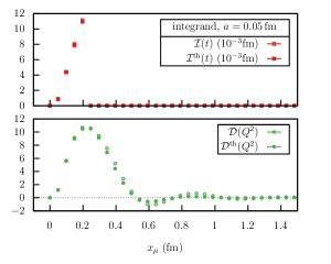
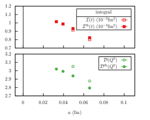
Figure 1: Left panel: Integrand of the fourth moment of the correlator (red squares) and the Adler function (green circles) at fixed lattice spacing. The vacuum and thermal observables are shown with open and filled symbols, respectively. Right panel: Corresponding integral as a function of the lattice spacing is shown, which illustrates that the thermal contribution with $T=250$ MeV accounts for most of the signal.

In particular, our strategy proposes to use the static screening correlator at finite temperature $T$,

$$G^{\mathrm{th}}(x_{3}) =-\int\mathrm{d}x_{0}\,\mathrm{d}x_{1}\,\mathrm{d}x_{2}\;\langle J^{\mathrm{em}}_{1}(x)J^{\mathrm{em}}_{1}(0)\rangle_{T},$$ (9)

which is a function of the spatial separation $x_{3}$ of the currents and depends on the temperature $T$. We choose the latter to be on the order of the QCD scale, in the chirally-restored phase. We define the contribution up to $t$ to the integral appearing in Eq. (3) for the vacuum and thermal correlators,

$$I({t}) =\int_{0}^{t}\mathrm{d}x_{0}\,x_{0}^{4}\,G(x_{0}),\qquad I^{\mathrm{th}}({t})=\int_{0}^{t}\mathrm{d}x_{3}\,x_{3}^{4}\,G^{\mathrm{th}}(x_{3}),$$ (10)

together with lattice estimators $\mathcal{I}(t,a)$ and its thermal counterpart $\mathcal{I}^{\mathrm{th}}(t,a)$ defined precisely in the following subsection.

Our strategy is based on the idea that the quantities $I({t})$ and $I^{\mathrm{th}}({t})$ are in some sense very similar. The operator-product expansion (OPE), which is presented in detail in Appendix A, can be invoked to make this statement precise for ${t}T\ll 1$: the difference of the two quantities is suppressed by $({t}T)^{3}$ relative to the quantities themselves. It is instructive to compare the thermal and the vacuum correlators in a representative lattice QCD calculation. The left panel of Figure 1 depicts the integrand of Eq. (10) with $t=0.2$ fm for the vacuum (open) and thermal (filled) squares at fixed lattice spacing $a\approx 0.05$ fm, which illustrates that the thermal effects are indeed suppressed for these distances in the $N_{\mathrm{f}}=2$ theory when $T=250$ MeV, corresponding to ${t}T=0.25$. The analogous integrands for the Adler function at the large virtuality of $Q=2.36$ GeV are shown as well, which illustrate how it is also dominated by the correlation function at short distances. The right-hand panel shows the corresponding integrals as a function of the lattice spacing, which illustrates that more than 95% of the signal is accounted for by the thermal observable. The benefit of using $I^{\mathrm{th}}({t})$ as a proxy for $I({t})$ is that, in the case illustrated in Figure 1, the finite-temperature ensemble has a factor eight fewer lattice sites than its vacuum counterpart due to its shorter time extent, which naively allows a span of a factor of $8^{1/4}\approx 1.68$ in the lattice spacing to be achieved for the thermal observable before the cost of obtaining the latter becomes comparable to the vacuum calculation.

Thus for a suitable choice of ${t}\ll 1/T$, we expect the bulk of the short-distance contribution to be given by the thermal component $I^{\mathrm{th}}({t})$, whose continuum limit can be obtained accurately thanks to the smaller lattice spacings accessible at finite temperature. This suggests an improved estimator for the vacuum observable

$$\widehat{\mathcal{I}}({t},a) =I^{\mathrm{th}}({t})+[\mathcal{I}({t},a)-\mathcal{I}^{\mathrm{th}}({t},a)],$$ (11)

where the first term on the right-hand side is the continuum estimate of the thermal observable, obtained using particularly fine lattice spacings available at high temperature. The remainder in brackets is small and of the form ${\rm const.}\times t^{5}(1+{\rm O}(t))$, where the constant is dominated by a momentum scale on the order of temperature. It is worth recording the parametric size of the cutoff effects on both terms: for the first term, the cutoff effects are of order $a^{2}$, while for the remainder, they are of order $a^{2}(Tt)^{3}$ in the O($a$)-improved theory. Thus, as long as the ratio of the lattice spacings used in the thermal theory to those used in the vacuum does not become as small as $(tT)^{3/2}$, which is the regime we have in mind, the cutoff effects on $\mathcal{I}^{\mathrm{th}}({t},a)$ are parametrically larger than the effects on the remainder. The upshot is that if $I(t)$ is obtained as the continuum limit of $\widehat{\mathcal{I}}({t},a)$, the dominant part of the systematic error associated with cutoff effects comes from obtaining $I^{\mathrm{th}}({t})$, where one profits from being able to reach lattice spacings below 0.05 fm in the chirally-restored phase at a moderate computational cost.

A further aspect which is specific to Wilson fermions is that the on-shell improvement of the vector current via the derivative of the tensor current Sint and Weisz (1997) only contributes a term of order $am_{\rm q}$ in the chiral restored phase of QCD; such terms are of a size comparable to the O($a^{2}$) terms for the lattice spacings employed in Section IV. This represents a further advantage of obtaining the bulk of $\widehat{\mathcal{I}}({t},a)$ from the chiral restored phase.

Since the main focus is then on obtaining $I^{\mathrm{th}}({t})$, it is worth studying the approach to the continuum for this short-distance quantity in lattice perturbation theory. The leading-order calculation is presented in Section III. It turns out that a logarithmic enhancement of the O($a^{2}$) cutoff effects arises, with a calculable coefficient which applies both to $I^{\mathrm{th}}({t})$ and $I({t})$. This enhancement appears with a positive (unit) power of the logarithm, unlike the known logarithmic dependence on the lattice spacing due to the running coupling, which appears first at one-loop level Husung et al. (2020). By contrast, the $\mathrm{O}(a^{2})$ cutoff effect enhanced by the factor $\log(1/a)$ cancels out in the improved observable (11).

In order to fully control the short-distance thermal contribution, or to reach very high momenta in the hadronic vacuum polarization, it may be necessary to iterate the procedure of Eq. (11) using a series of higher temperatures to compute short-distance contributions. We return to this question in Section V. Although other options are certainly available, it is particularly convenient to use the temperature as a control parameter to compute the short-distance contribution, since we can use existing knowledge about high-temperature correlators and apply well-understood theoretical tools like the operator product expansion.

II.1 Definitions of lattice observables

In order to set up the notation for the following sections, we define here the lattice observables for the theory of $N_{\mathrm{f}}=2$ Wilson fermions. In this work we investigate the isovector vector current correlator, which consists of a single Wick contraction. This correlator makes the dominant contribution to the hadronic vacuum polarization in the muon $g-2$. In the vacuum case, we formulate the correlator at vanishing spatial momentum as a function of Euclidean time,

$$\mathcal{G}_{\mu\nu}(x_{0}) =Z_{\mathrm{V}}(1+am_{\mathrm{q}}b_{\mathrm{V}})a^{3}\sum_{\bm{x}}\langle\widetilde{V}_{\mu}(x)V_{\nu}(0)\rangle\;,$$ (12)

where the bare local vector current is defined as

$$V_{\mu}(x) =\bar{\Psi}(x)\frac{\tau_{3}}{\sqrt{2}}\gamma_{\mu}\Psi(x)$$ (13)

with $\Psi^{\top}=(u,d)$, and the exactly-conserved vector current is

$$\widetilde{V}_{\mu}(x) =\frac{1}{2}\big{[}\bar{\Psi}(x+a\hat{\mu})\frac{\tau_{3}}{\sqrt{2}}(1+\gamma_{\mu})U^{\dagger}_{\mu}(x)\Psi(x)-\bar{\Psi}(x)\frac{\tau_{3}}{\sqrt{2}}(1-\gamma_{\mu})U_{\mu}(x)\Psi(x+a\hat{\mu})\Big{]}.$$ (14)

In contrast, the static screening correlator at finite temperature is measured along a spatial direction,

$$\mathcal{G}^{\mathrm{th}}_{\mu\nu}(x_{3}) =Z_{\mathrm{V}}(1+am_{\mathrm{q}}b_{\mathrm{V}})a^{3}\sum_{x_{0}}\sum_{x_{1},x_{2}}\langle\widetilde{V}_{\mu}(x)V_{\nu}(0)\rangle_{T}$$ (15)

We investigate two observables which are related to the Adler function Eq. (1), and the short-distance part of the fourth moment of the correlator Eq. (10), which is proportional to the derivative of the vacuum polarization at zero virtuality. The short-distance contribution up to $t$ of the fourth moment is

$$\mathcal{I}({t}) =a\sum_{x_{0}=a}^{{t}-a}x_{0}^{4}\,\mathcal{G}(x_{0})+\frac{a}{2}{t}^{4}\,\mathcal{G}({t}),\qquad\mathcal{G}\equiv-\mathcal{G}_{11}.$$ (16)

We have used an integration rule consistent with the improvement of the theory, e.g. the trapezoidal rule. For large $Q^{2}$, the Adler function is dominated by the short-distance contribution to the integral, and we define a lattice observable which is the integral up to half the spatial extent $L/2$,

$$\mathcal{D}(Q^{2}) =a\sum_{x_{0}=a}^{L/2-a}K(x_{0},Q^{2})\mathcal{G}(x_{0})+\frac{a}{2}K(L/2,Q^{2})\mathcal{G}(L/2),$$ (17)

where again we have implemented the trapezoidal rule, and $K(x_{0},Q^{2})$ is defined in Eq. (2). The thermal observables are defined analogously using the static screening correlator of Eq. (15). The improved estimators are then defined via Eq. (11) where the first term on the right-hand side is obtained by taking the continuum limit using thermal ensembles with the available finer lattice spacings.

II.2 The Symanzik expansion and enhanced lattice artifacts

As discussed at the beginning of the section (see Eqs. (6-7)), severe lattice artifacts appear in the correlation function at short distances. Here, we demonstrate that integrating over the correlation function with a kernel suppressing the short distances sufficiently so as to yield a finite continuum limit can result in a parametric enhancement of lattice artifacts even at leading order in the perturbative expansion.

The Symanzik continuum effective theory can be used to represent the correlation function on the lattice for $x_{0}>0$ by considering all irrelevant counterterms of the action and local operators with the correct dimension and consistent with the symmetries of the lattice theory. For example, the lattice artifacts of Eq. (7) can be expressed as a sum over the matrix elements containing the counterterms Husung et al. (2020)

$$\mathcal{G}_{n}(x_{0},a) =\sum_{i}\bar{c}^{i}\{2b_{0}\bar{g}^{2}(\tfrac{1}{a})\}^{\hat{\gamma}^{i}}\mathcal{C}^{i}_{n}(x_{0}),\qquad\hat{\gamma}^{i}=\gamma_{0}^{i}/b_{0},$$ (18)

with coefficients which depend on the (scheme-independent) one-loop anomalous dimension of the counterterm $\gamma_{0}^{i}$ ($b_{0}$ is the universal one-loop coefficient of the QCD beta function) and $\bar{c}^{i}$ is the matching coefficient between the Symanzik continuum effective theory and the lattice theory. The matrix element $\mathcal{C}_{n}^{i}$ is renormalization-group invariant as the scale-dependence of the counterterm has been factored out, which gives rise to a logarithmic dependence on the lattice spacing through the running coupling.

In addition, however, the integral of the correlator from short-distances results in a logarithmically-enhanced lattice artifact. In Eq. (7), the matrix element of any one of the leading $\mathrm{O}(a^{2})$ counterterms must have by power counting the short-distance singularity

$$\mathcal{C}^{i}_{2}(x_{0}) =d^{i}(1/x_{0})^{5}+\ldots.$$ (19)

This is more singular than the leading continuum correlator, and gives rise to a logarithmic enhancement of the O($a^{2}$) lattice artifacts in the $x_{0}^{4}$ moment, in particular when inserted in the summation of Eq. (16), using the harmonic number formula. Thus, assuming the correlator is O($a$)-improved, the leading $\mathrm{O}(a^{2})$ lattice artifacts of the integrated quantity are parametrically enhanced due to the logarithm appearing with the (positive) unit power. It is also worth noting that all higher terms in the Symanzik expansion of ${\cal G}(x_{0},a)$ contribute at O($a^{2}$) after summing over short distances. In particular, even if one improved the on-shell correlator so that it contained no O($a^{2}$) artifacts, the quantity ${\cal I}(x_{0},a)$ would contain remnant O($a^{2}$) lattice artifacts.

The full form of the lattice artifacts given by Eq. (18) suggests that the coefficient of the logarithmic term could be determined by computing all of the matching, or improvement, coefficients while the most singular behaviour of the coefficient function is computable in continuum perturbation theory, when $x_{0}\Lambda\ll 1$. In the following section, the coefficient of the logarithmically-enhanced term is computed at leading order in lattice perturbation theory.

III Analysis in leading order of lattice perturbation theory

As a first test of the idea to use thermal gauge ensembles to better control the short-distance behaviour of QCD correlators, we apply it in the framework of leading-order lattice perturbation theory, i.e. in the theory of non-interacting quarks. In the limit of short distances, the QCD correlation functions are well approximated by their perturbative values, and we therefore expect the free theory to provide valuable insight on the general applicability of the method. Moreover, the continuum values being known in this context, quantitative statements can be made about the accuracy of the continuum limit obtained with the improved estimators in Eq. (11) as compared to extrapolating directly the vacuum observables.

One delicate point in the study of the integrated observables defined in Section II.1 is the presence, already at the level of the free theory, of cutoff effects which depend logarithmically on the lattice spacing. In the method we propose, the understanding of these effects is important in view of obtaining an accurate continuum extrapolation of the thermal observables. On the other hand, the improved vacuum observables defined as in Eq. (11) are free of the logarithm predicted by the leading-order calculation, which cancel out in the subtraction between thermal and vacuum quantities.

III.1 The vector correlators in the massless theory: lattice formulation

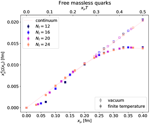
Figure 2: Integrand of the fourth-moment observable $x_{\mu}^{4}\mathcal{G}(x_{\mu})$ for four thermal lattices with $N_{t}=12,16,20,24$ (filled symbols) and their vacuum equivalents (open symbols). The dotted lines represent the continuum values of these quantities.

We consider the theory of non-interacting massless Wilson quarks, defined on a lattice with infinite spatial volume. Following Section II.1, we denote the lattice vacuum and thermal correlation functions by $\mathcal{G}_{\mu\nu}(x_{0})$ and $\mathcal{G}^{\mathrm{th}}_{\mu\nu}(x_{3})$ (Eqs. (12) and (15), recalling that $Z_{\mathrm{V}}=1$ in the non-interacting case). Explicit expressions of the free correlators are given in Appendix D for the theory with $N_{c}$ colors. Here we fix $N_{c}=3$, as appropriate for QCD. We concentrate on the observables $\mathcal{I}(t)$ and $\mathcal{D}(Q^{2})$, as defined in Eqs. (16) and (17).

The analysis is performed at a set of realistic lattice spacings which correspond to those available in our non-perturbative study of $N_{f}=2$ QCD (see Table 4). In the free massless Lagrangian there are no bare parameters to be tuned in order to approach the continuum on a line of constant physics, given that the mass parameter is only multiplicatively renormalized in this case. The fact that the non-interacting massless theory is scale invariant gives us the freedom to assign to the temperature a value of our choice. In the thermal case, the lattice spacing and the temperature are related by $T=1/(aN_{t})$, where $N_{t}=L_{0}/a$ is the number of lattice points in the Euclidean-time direction. As in the case of the interacting ensembles, we consider four finite-temperature lattices, with $N_{t}=12,16,20,24$, and we assign to each of them the physical temperature $T=246.25$ MeV, which corresponds to fixing the lattice extent in the compact direction to $aN_{t}=1/T=0.8$ fm. This results in the set of lattice spacings $a\approx\{0.07,0.05,0.04,0.03\}$ fm. Vacuum equivalents of these thermal systems are obtained by assigning the corresponding physical value of the lattice spacing to a lattice with $N_{t}=\infty$ (zero temperature). For simplicity, with an abuse of notation we will sometimes identify the vacuum lattices by the value of $N_{t}$ of their thermal counterpart (as for example in Figure 4). We analyze $\mathcal{I}(t)$ for $t=1/(4T)=0.2$ fm and $t=1/(2T)=0.4$ fm, and for the Adler function we consider the two virtualities $Q=3\pi T=2.32$ GeV and $Q=\pi T/2=387$ MeV. We are mostly interested in the more short-distance-dominated cases $t=0.2$ fm and $Q=2.32$ GeV, for which the method proposed in this paper proves to be very effective. Similar values of $t$ and $Q$ are used in the analysis of the $N_{f}=2$ QCD data presented in Section IV. The more infrared scales $t=0.4$ fm and $Q=387$ MeV are only considered in the free-theory analysis, and they mostly serve as a comparison point.

Figure 2 shows the integrand of the fourth-moment observable $x_{\mu}^{4}\mathcal{G}(x_{\mu})$ for all thermal lattices and their vacuum counterparts, up to distances of $0.4$ fm. As expected, up to around 0.2 fm the difference between the vacuum and thermal cases is hardly noticeable. Also, at these short distances the cutoff effects are more important than at larger separations, as can be observed by comparing with the continuum values, also displayed in the plot. These two features motivate the use of the improved observables defined as in Eq. (11) in order to achieve a better control at short distances with the aid of fine thermal lattices.

Before undertaking the analysis of the observables $\mathcal{I}(t)$ and $\mathcal{D}(Q^{2})$ with the method proposed in this paper, we investigate the emergence of logarithmic cutoff effects and compute their form explicitly.

III.2 A short-distance O$(a^{2}\log(1/a))$ cutoff effect

Already at the free-theory level, cutoff effects of the form $\tilde{c}\>a^{2}\log(1/a)$ are present in the observables $\mathcal{I}(t)$ and $\mathcal{D}(Q^{2})$,

$$\mathcal{I}(t)\overset{a\to 0}{\sim}I(t)+\tilde{c}_{\mathcal{I}}a^{2}\log(1/a)+O(a^{2})\>,$$ (20)

$$\mathcal{D}(Q^{2})\overset{a\to 0}{\sim}D(Q^{2})+\tilde{c}_{\mathcal{D}}a^{2}\log(1/a)+O(a^{2})\>,$$ (21)

and analogously in the corresponding thermal quantities $\mathcal{I}^{\mathrm{th}}(t)$ and $\mathcal{D}^{\mathrm{th}}(Q^{2})$. In the following we compute the coefficients $\tilde{c}_{\mathcal{I}}$ and $\tilde{c}_{\mathcal{D}}$ for the specific discretization of the correlation functions used in this work.

To begin with, we focus on $\mathcal{I}(t)$ and we analyze it in the limit $a\to 0$. In the vacuum and in infinite volume there is no difference between projecting to zero momentum in the directions $(x_{1},x_{2},x_{3})$, as in Eq. (12), or in the directions $(x_{0},x_{1},x_{2})$. Here, as in Appendix D, we choose the second option, as it makes the analogy with the thermal screening correlator very clear. As a consequence, we will use the vector notation $\bm{p}\equiv(p_{0},p_{1},p_{2})$. The thermal version of the following equations is obtained by replacing the integral over $p_{0}$ with a sum over fermionic Matsubara modes, as described in Appendix D, and the coefficients $\tilde{c}_{\mathcal{I}}$ and $\tilde{c}_{\mathcal{D}}$ are the same in the vacuum and in the thermal case. In the limit $a\to 0$, the observable $\mathcal{I}(t)$ can be expanded as follows,

$$\begin{split}\mathcal{I}(t)=\int_{0}^{t}\mathrm{d}x_{3}\>x_{3}^{4}\int_{-\frac{\pi}{a}}^{\frac{\pi}{a}}\frac{\mathrm{d}^{3}p}{(2\pi)^{3}}\>e^{-2p\absolutevalue{x_{3}}}\biggl{[}\hat{f}_{0,0}(\hat{\bm{p}})\>+a^{2}\bigl{(}p^{2}\hat{f}_{2,0}(\hat{\bm{p}})+\absolutevalue{x_{3}}p^{3}\hat{f}_{2,1}(\hat{\bm{p}})\bigr{)}+O(a^{4})\biggr{]}+O(a^{2})\>,\end{split}$$ (22)

where $p\equiv\absolutevalue{\bm{p}}$ and $\hat{f}_{n,m}(\hat{\bm{p}})$ are dimensionless functions of the orientation of the vector $\bm{p}$ ($\hat{\bm{p}}\equiv\bm{p}/p$). The expressions of $\hat{f}_{00}$, $\hat{f}_{2,0}$ and $\hat{f}_{2,1}$ can be found in Appendix D. A generic term of the expansion within square brackets in (22) can be expressed as

$$a^{n}\absolutevalue{x_{3}}^{m}p^{n+m}\hat{f}_{n,m}(\hat{\bm{p}})\>,$$ (23)

with $n=2,4,\dots$ and $m\geq 0$. The integration over $x_{3}$ yields

$$\int_{0}^{t}\mathrm{d}x_{3}\>x_{3}^{m+4}\>e^{-2px_{3}}=\frac{(m+4)!}{(2p)^{m+5}}-e^{-2pt}\sum_{l=0}^{m+4}\frac{(m+4)!}{(m+4-l)!}\frac{t^{m+4-l}}{(2p)^{l+1}}\>.$$ (24)

Upon integration over the Brillouin zone, the first term on the right-hand-side of Eq. (24) (not exponentially suppressed in $p$) can introduce a logarithmic dependence on $a$. In fact, based on dimensional analysis, we observe that the term

$$\mathcal{I}(t)\supset a^{n}\frac{(m+4)!}{2^{m+5}}\int_{-\frac{\pi}{a}}^{\frac{\pi}{a}}\frac{\mathrm{d}^{3}p}{(2\pi)^{3}}\frac{\hat{f}_{n,m}(\hat{\bm{p}})}{p^{5-n}}$$ (25)

is proportional to $a^{2}\log(1/a)$ for $n=2$, and to $a^{2}$ for any $n>2$. As a consequence, the $O(a^{2})$ contribution to $\mathcal{I}(t)$ cannot be computed exactly by truncating the expansion in square brackets in Eq. (22) at a finite order. Having identified the sources of logarithmic contributions, we can compute the coefficient $\tilde{c}_{\mathcal{I}}$ by using the log-derivative

$$\tilde{c}_{\mathcal{I}}=\frac{1}{a}\frac{\mathrm{d}}{\mathrm{d}(1/a)}\int_{-\frac{\pi}{a}}^{\frac{\pi}{a}}\frac{\mathrm{d}^{3}p}{(2\pi)^{3}}\frac{1}{p^{3}}\biggl{\{}\frac{4!}{2^{5}}\hat{f}_{2,0}(\hat{\bm{p}})+\frac{5!}{2^{6}}\hat{f}_{2,1}(\hat{\bm{p}})\biggl{\}}\biggr{\rvert}_{a=0}\>.$$ (26)

The derivative of the triple integral can be computed by applying the following equation

$$\frac{\mathrm{d}}{\mathrm{d}x}\int_{0}^{x}\mathrm{d}^{3}p\>f(p_{0},p_{1},p_{2})=\int_{0}^{x}\mathrm{d}^{2}p\>\bigl{[}f(p_{0},p_{1},x)+f(p_{0},x,p_{1})+f(x,p_{0},p_{1})\bigr{]}\>.$$ (27)

Using the expressions of $\hat{f}_{2,0}$ and $\hat{f}_{2,1}$ given in Appendix D, we find

$$\tilde{c}_{\mathcal{I}}=\frac{7N_{c}}{60\pi^{2}}\overset{N_{c}=3}{=}\frac{7}{20\pi^{2}}\>.$$ (28)

Table 1: Parameters of the continuum extrapolation of $\mathcal{I}^{\mathrm{th}}(t)$ and $\mathcal{D}^{\mathrm{th}}(Q^{2})$ with the functional forms $(a)$, $(b)$, $(c)$, $(d)$ of Eq. (31). The known continuum values $I^{\mathrm{th}}(t)$ and $D^{\mathrm{th}}(Q^{2})$ are also reported, together with the prefactors of the logarithmic term $\tilde{c}_{\mathcal{I}}$ (Eq. (28)) and $\tilde{c}_{\mathcal{D}}$ (Eq. (30)). For this analysis an extended set of thermal lattices is used, with $N_{t}=16,20,24,48,60,120$ and whose temperature is fixed to $T=246.25$ MeV. For all fit forms, $c_{0}$ is in good agreement with the corresponding continuum value. In the more infrared cases $t=0.4$ fm and $Q=387$ MeV the ansatz $(a)$ provides a good estimate of $\tilde{c}$, and the value of this coefficient is quite stable with respect to introducing higher powers of $a$ in the fit ansatz. Instead for $t=0.2$ fm and $Q=2.32$ GeV the role of higher-order discretization effects is important to obtain a relatively accurate estimate of $\tilde{c}$. In particular, among the fit forms analyzed here, the ansatz $(c)$ provides the most accurate value.

Free massless quarks
$t$ [fm]	$I^{\mathrm{th}}(t)\leavevmode\nobreak\ [10^{-3}\mathrm{fm}^{2}]$	$\tilde{c}_{\mathcal{I}}$	$c_{0}\leavevmode\nobreak\ [10^{-3}\mathrm{fm}^{2}]$	$\tilde{c}$	$c_{2}$	$c_{3}\leavevmode\nobreak\ [\mathrm{fm}^{-1}]$	$c_{4}\leavevmode\nobreak\ [\mathrm{fm}^{-2}]$
0.2	1.025	0.0355	1.026	0.0251	$-0.112$	–	–	$(a)$
			1.025	0.0466	$-0.197$	0.522	–	$(b)$
			1.025	0.0377	$-0.156$	–	3.70	$(c)$
			1.025	0.0292	$-0.116$	$-0.488$	7.13	$(d)$
0.4	3.603	0.0355	3.603	0.0332	$-0.123$	–	–	$(a)$
			3.603	0.0373	$-0.139$	0.0992	–	$(b)$
			3.603	0.0356	$-0.132$	–	0.703	$(c)$
			3.603	0.0352	$-0.130$	$-0.0231$	0.866	$(d)$
$Q$ [GeV]	$D^{\mathrm{th}}(Q^{2})$	$\tilde{c}_{\mathcal{D}}[\mathrm{fm}^{-2}]$	$c_{0}$	$\tilde{c}\leavevmode\nobreak\ [\mathrm{fm}^{-2}]$	$c_{2}\leavevmode\nobreak\ [\mathrm{fm}^{-2}]$	$c_{3}\leavevmode\nobreak\ [\mathrm{fm}^{-3}]$	$c_{4}\leavevmode\nobreak\ [\mathrm{fm}^{-4}]$
2.32	2.695	48.6	2.697	30.8	$-138$	–	–	$(a)$
			2.695	56.7	$-241$	639	–	$(b)$
			2.695	45.8	$-190$	–	4518	$(c)$
			2.695	52.1	$-219$	369	1916	$(d)$
0.387	0.2927	1.349	0.2927	1.320	$-2.57$	–	–	$(a)$
			0.2927	1.368	$-2.76$	1.19	–	$(b)$
			0.2927	1.348	$-2.67$	–	8.46	$(c)$
			0.2927	1.350	$-2.67$	0.108	7.70	$(d)$

Moving now to the Adler function $\mathcal{D}(Q^{2})$, we observe that in the short-distance limit its integrand is proportional to that of $\mathcal{I}(t)$

$$K(x_{3},Q^{2})\mathcal{G}(x_{3})\overset{x_{3}\to 0}{\sim}\pi^{2}Q^{2}\>x_{3}^{4}\>\mathcal{G}(x_{3})\>.$$ (29)

As we saw in the above computation, the logarithmic cutoff effect comes from the contribution around $x_{3}=0$ to the integral over $x_{3}$ (see Eq. (24)), from which we conclude that

$$\tilde{c}_{\mathcal{D}}=\pi^{2}Q^{2}\>\tilde{c}_{\mathcal{I}}=\frac{7N_{c}Q^{2}}{60}\overset{N_{c}=3}{=}\frac{7Q^{2}}{20}\>.$$ (30)

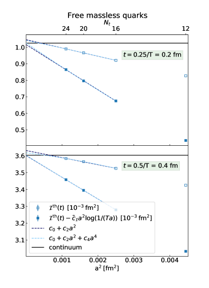
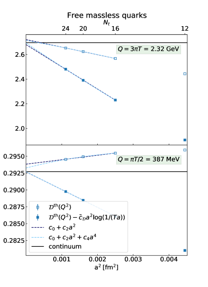
Figure 3: Continuum limit of the thermal quantities $\mathcal{I}^{\mathrm{th}}(t)$ (left) and $\mathcal{D}^{\mathrm{th}}(Q^{2})$ (right). Four lattices are considered, with $N_{t}=12,16,20,24$ and whose temperature is fixed to 264.25 MeV. The coarsest lattice with $N_{t}=12$ is excluded from the fits. Polynomials of first and second degree in $a^{2}$ are used to fit the data. More accurate extrapolations are obtained by making use of the known coefficients $\tilde{c}_{\mathcal{I}}$ (28) and $\tilde{c}_{\mathcal{D}}$ (30) to subtract the $O(a^{2}\log(1/a))$ contribution from the lattice data. The relative differences between the continuum estimates shown in this figure and the correct continuum values are listed in Table 2.

The values of $\tilde{c}_{\mathcal{I}}$ and $\tilde{c}_{\mathcal{D}}$ given in Eqs. (28) and (30) can be compared to what is obtained via fits to the lattice data. With this goal in mind, we consider a set of lattices with $N_{t}=16,20,24,48,60,120$, whose temperature is fixed to $T=246.25$ MeV. These include “realistic” lattices with $N_{t}=16,20,24$, whose lattice spacings are very close to those of the ensembles presented in Section IV, and three extremely fine lattices with $N_{t}=48,60,120$. We include the latter in order to have a better control on the continuum extrapolation and more flexibility with respect to the number of fit parameters. We consider the functional forms

$$\begin{split}&(a)\quad c_{0}+a^{2}[c_{2}+\tilde{c}\log(1/(Ta))]\\ &(b)\quad c_{0}+a^{2}[c_{2}+\tilde{c}\log(1/(Ta))]+c_{3}a^{3}\\ &(c)\quad c_{0}+a^{2}[c_{2}+\tilde{c}\log(1/(Ta))]+c_{4}a^{4}\\ &(d)\quad c_{0}+a^{2}[c_{2}+\tilde{c}\log(1/(Ta))]+c_{3}a^{3}+c_{4}a^{4}\\ \end{split}$$ (31)

and observe that the case $(c)$ leads to the best agreement with the expected value of $\tilde{c}$. In all cases, the agreement between $c_{0}$ and the known continuum value is very good. All results are reported in Table 1.

III.3 Continuum limit of the thermal observables

Table 2: Accuracy of the continuum limit of $\mathcal{I}^{\mathrm{th}}(t)$ (left) and $\mathcal{D}^{\mathrm{th}}(Q^{2})$ (right) expressed in terms of the relative difference between the continuum estimate $c_{0}$ and the known continuum value. Three thermal lattices are used for the extrapolation, with $N_{t}=16,20,24$ and whose temperature is set to $T=246.25$ MeV. The label ‘plain’ refers to a continuum estimate obtained by fitting the plain lattice observables $\mathcal{I}^{\mathrm{th}}(t)$ and $\mathcal{D}^{\mathrm{th}}(Q^{2})$, while in the case ‘subtr.’ the logarithmic cutoff effects are subtracted prior to performing the fit as follows, $\mathcal{I}^{\mathrm{th}}(t)-\tilde{c}_{\mathcal{I}}a^{2}\log(1/(Ta))$, $\mathcal{D}^{\mathrm{th}}(Q^{2})-\tilde{c}_{\mathcal{D}}a^{2}\log(1/(Ta))$. The analytic values of the coefficients $\tilde{c}_{\mathcal{I}}$ and $\tilde{c}_{\mathcal{D}}$ are given in Eqs. (28) and (30) respectively. The lattice data and the fit curves are shown in Figure 3.

Free massless quarks
$t$ [fm] $\absolutevalue{c_{0}-I^{\mathrm{th}}(t)}/I^{\mathrm{th}}(t)$ ansatz 0.2 2% 0.9% $c_{0}+c_{2}a^{2}$ 2% 0.2 % $c_{0}+c_{2}a^{2}+c_{4}a^{4}$ 0.4 0.8% 0.06 % $c_{0}+c_{2}a^{2}$ 0.4% < 0.01% $c_{0}+c_{2}a^{2}+c_{4}a^{4}$ plain subtr.    $Q$ [GeV] $\absolutevalue{c_{0}-D^{\mathrm{th}}(Q^{2})}/D^{\mathrm{th}}(Q^{2})$ ansatz 2.32 0.9% 0.6% $c_{0}+c_{2}a^{2}$ 0.7% 0.06 % $c_{0}+c_{2}a^{2}+c_{4}a^{4}$ 0.387 0.4% < 0.01% $c_{0}+c_{2}a^{2}$ 0.2% < 0.01% $c_{0}+c_{2}a^{2}+c_{4}a^{4}$ plain subtr.

As a first step toward improved vacuum observables defined as in Eq. (11), we compute continuum estimates of the thermal quantities $\mathcal{I}^{\mathrm{th}}(t)$ and $\mathcal{D}^{\mathrm{th}}(Q^{2})$. We consider a set of four lattices with $N_{t}=12,16,20,24$, whose temperature is set to 246.25 MeV and whose lattice spacings are very similar to the ones of the $N_{f}=2$ thermal ensembles, as discussed in Section III.1. In all practical cases, we find it expedient to exclude the coarser lattice with $N_{t}=12$ from the continuum extrapolation.

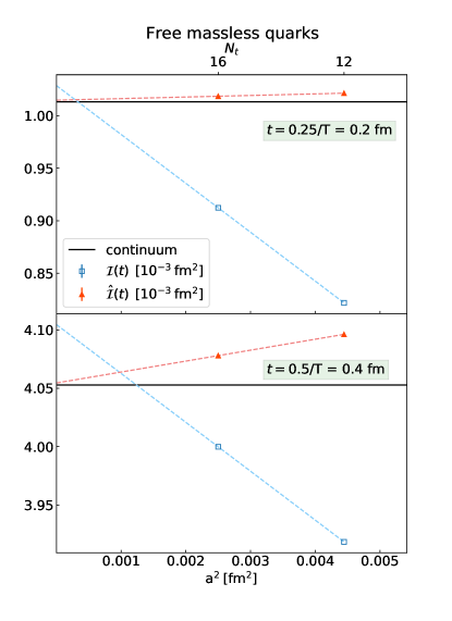
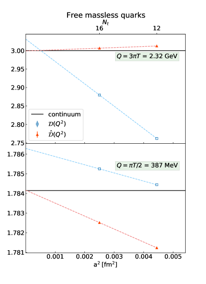
Figure 4: Continuum extrapolation of the vacuum lattice observables $\mathcal{I}(t)$ (left) and $\mathcal{D}(Q^{2})$ (right) and of their improved versions $\hat{\mathcal{I}}(t)$ and $\hat{\mathcal{D}}(Q^{2})$. The observables are evaluated on two lattices whose lattice spacings $a\approx\{0.07,0.05\}$ fm are equal to those of the $N_{t}=12,16$ thermal lattices. The fit ansatz is linear in $a^{2}$. The accuracy of the resulting continuum estimates is reported in Table 3.

We observe that a careful treatment of the logarithmic cutoff effects can significantly improve the accuracy of the continuum limit. In order to illustrate this point, we compare the outcome of two different approaches. The first is to simply ignore the presence of logarithmic cutoff effects and to fit the lattice data with polynomials in $a^{2}$. The second is to subtract the logarithmic contributions making use of the known prefactors $\tilde{c}_{\mathcal{I}}$ and $\tilde{c}_{\mathcal{D}}$ (see Section III.2) before fitting polynomially in $a^{2}$. This second approach proves to be very effective, however it is somewhat specific to the free theory. In the interacting case, it remains to be seen whether the $a^{2}\log(1/a)$ term receives significant, non-analytic in $a$ corrections. Another possible strategy is to fit the lattice data with the ansatz $c_{0}+c_{2}a^{2}+\tilde{c}a^{2}\log(1/(Ta))$. In this case we find that the accuracy of the continuum estimates is comparable with the results obtained by subtracting the logarithmic term and then fitting linearly in $a^{2}$, which are given in Table 2.

In the left panel of Figure 3 two sets of lattice data are shown, one corresponds to the plain thermal observable $\mathcal{I}^{\mathrm{th}}(t)$ (open symbols) and the other represents $\mathcal{I}^{\mathrm{th}}(t)-\tilde{c}_{\mathcal{I}}a^{2}\log(1/(Ta))$ (filled symbols). The value of the coefficient $\tilde{c}_{\mathcal{I}}$ is given in Eq. (28). Four different continuum estimates are obtained by fitting these data sets with two polynomial forms, one linear in $a^{2}$ and one quadratic in the same variable. The discrepancy between these estimates and the known continuum value is reported on the left-hand side of Table 2. The accuracy of the continuum limit is significantly improved by the subtraction of the logarithmic term and the inclusion of the $O(a^{4})$ term also plays an important role. For example, for $t=0.2$ fm a naive polynomial fit of the lattice data gives a discrepancy with the correct continuum value of around $2\%$, which is reduced to $0.2\%$ by subtracting the logarithmic cutoff effects and fitting the resulting lattice points with a second-degree polynomial in $a^{2}$. As final continuum estimates we choose the most accurate results

$$I^{\mathrm{th}}_{\mathrm{extrap.}}(t=0.2\leavevmode\nobreak\ \mathrm{fm})=1.027\times 10^{-3}\leavevmode\nobreak\ \mathrm{fm}^{2}\>,\quad I^{\mathrm{th}}_{\mathrm{extrap.}}(t=0.4\leavevmode\nobreak\ \mathrm{fm})=3.603\times 10^{-3}\leavevmode\nobreak\ \mathrm{fm}^{2}\>.$$ (32)

A similar analysis of the thermal Adler function $\mathcal{D}^{\mathrm{th}}(Q^{2})$ can be found on the right panel of Figure 3 and on the right-hand side of Table 2. Also for this observable the gain in accuracy due to subtracting the logarithmic cutoff effects is considerable. For example, for $Q=2.32$ GeV the continuum estimate obtained by fitting $\mathcal{D}^{\mathrm{th}}(Q^{2})$ with a second-degree polynomial in $a^{2}$ differs from the correct continuum value by $0.7\%$, while fitting $\mathcal{D}^{\mathrm{th}}(Q^{2})-\tilde{c}_{\mathcal{D}}a^{2}\log(1/(Ta))$ with the same ansatz reduces the discrepancy to $0.06\%$. The value of $\tilde{c}_{\mathcal{D}}$ is given in Eq. (30). As final continuum estimates of the thermal Adler function we choose the most accurate values

$$D^{\mathrm{th}}_{\mathrm{extrap.}}(Q=2.32\leavevmode\nobreak\ \mathrm{GeV})=2.694\>,\quad D^{\mathrm{th}}_{\mathrm{extrap.}}(Q=387\leavevmode\nobreak\ \mathrm{MeV})=0.2927\>.$$ (33)

Table 3: Accuracy of the continuum estimates obtained by fitting with the ansatz $c_{0}+c_{2}a^{2}$ the lattice observables $\mathcal{I}(t)$, $\mathcal{D}(Q^{2})$ and their improved versions $\hat{\mathcal{I}}(t)$, $\hat{\mathcal{D}}(Q^{2})$ defined in Eqs. (34) and (35). The accuracy is expressed in terms of the relative difference with the known continuum values $I(t)$ and $D(Q^{2})$. The lattice data and the fit curves are shown in Figure 4.

Free massless quarks
$t$ [fm] $\absolutevalue{c_{0}-I(t)}/I(t)$ 0.2 2% 0.2% 0.4 1% 0.04 % $\mathcal{I}$ $\hat{\mathcal{I}}$       $Q$ [GeV] $\absolutevalue{c_{0}-D(Q^{2})}/D(Q^{2})$ 2.32 1% 0.03% 0.387 0.1% < 0.01% $\mathcal{D}$ $\hat{\mathcal{D}}$

III.4 Continuum limit of the improved vacuum observables

With the continuum estimates of Eqs. (32) and (33), we build the improved vacuum observables

$$\hat{\mathcal{I}}(t)=I^{\mathrm{th}}_{\mathrm{extrap.}}(t)+[\mathcal{I}(t)-\mathcal{I}^{\mathrm{th}}(t)]\>,$$ (34)

$$\hat{\mathcal{D}}(Q^{2})=D^{\mathrm{th}}_{\mathrm{extrap.}}(Q^{2})+[\mathcal{D}(Q^{2})-\mathcal{D}^{\mathrm{th}}(Q^{2})]\>.$$ (35)

As in the case of the $N_{f}=2$ QCD ensembles, we evaluate the observables on two zero-temperature lattices, whose lattice spacings $a\approx\{0.07,0.05\}$ fm are the same as those of the $N_{t}=12,16$ thermal lattices. We obtain continuum estimates by fitting linearly in $a^{2}$ the lattice observables $\mathcal{I}(t)$, $\mathcal{D}(Q^{2})$ and their improved versions defined in Eqs. (34) and (35). The lattice data and the fit curves are shown in Figure 4, while the accuracy of the resulting continuum estimates, given in terms of the relative difference with the correct continuum value, is reported in Table 3. For the case of $\mathcal{I}(t=0.2\,{\rm fm})$, one order of magnitude in accuracy is gained by using the improved lattice observables introduced in this paper.

In all cases considered here, the advantage of using the improved observables $\hat{\mathcal{I}}(t)$, $\hat{\mathcal{D}}(Q^{2})$ is rather clear as far as the accuracy of the resulting continuum estimates is concerned. For the more ultraviolet scales $t=0.2$ fm and $Q=2.32$ GeV there is the further benefit of a significant reduction of the cutoff effects at finite lattice spacing, as compared to the plain lattice observables $\mathcal{I}(t)$, $\mathcal{D}(Q^{2})$. As a final remark, we repeat that the logarithmic discretization effects proportional to $a^{2}\log(1/a)$ cancel in $\hat{\mathcal{I}}(t)$ and $\hat{\mathcal{D}}(Q^{2})$, due to the subtraction between the vacuum and thermal lattice observables.

IV Non-perturbative test in $N_{\mathrm{f}}=2$ QCD

In this section, we perform a non-perturbative numerical study of the same observables investigated in the free theory in the previous section, namely the (truncated) fourth moment of the current correlator and the Adler function at large virtuality. We make use of the vacuum CLS ensembles with $N_{\mathrm{f}}=2$ non-perturbatively O($a$)-improved Wilson fermions and the Wilson gauge action with two lattice spacings of $a\approx 0.049$ fm and $a=0.0658$ fm. Our study is performed at a fixed, common mass of the up and down quarks. For the (zero-temperature) pion mass, we quote the values 268(3) MeV and 269(3) MeV respectively for ensembles F7 and O7 Engel et al. (2015). The improved estimators were computed using ensembles on the same line of constant physics set by the physical volume $L$ and quark mass $m_{\mathrm{q}}$ with a temperature of $T=250$ MeV.

The aspect ratio for the finite-temperature ensembles was set to $L_{0}/L=1/4$, and for the vacuum ensembles to $L_{0}/L=2$. The thermal ensembles were recently used in a study of the photon emissivity of the quark-gluon plasma Cè et al. (2020). Two of them have common bare parameters with the vacuum ensembles, while two additional ensembles with lattice spacings down to $a\simeq 0.033$ fm allow the continuum limit of the thermal observable to be obtained with reduced uncertainty. Further details on the ensembles are collected in Table 4. The scale was set for the F7 ensemble taking the lattice spacing from ref. Fritzsch et al. (2012), and assuming a perfect line of constant physics with a ratio of lattice spacings of 3/4 between O7 and F7. The assumed ratio of lattice spacings is consistent at the one-sigma level with the values of the lattice spacings given in Fritzsch et al. (2012), as well as with those of Ref. Engel et al. (2015), in which they are quoted with a 0.9% precision. Note that in contrast to the free massless theory, in the present case the current is not fully O($a$)-improved as the improvement coefficients are not known non-perturbatively. Nevertheless, at high temperature, the O($a$) discretization effects due to the missing current improvement terms should be proportional to the quark mass O($am_{\mathrm{q}})$, owing to the restoration of chiral symmetry in the massless theory Dalla Brida et al. (2020); Brandt et al. (2018).

Table 4: Simulation parameters for the investigation with $N_{\mathrm{f}}=2$ non-perturbatively O($a$)-improved Wilson fermions. For the ensembles W7 and X7, the tuning to the line of constant physics defined by the temperature and the quark mass was performed in Ref. Steinberg (2021) using the Schrödinger functional coupling computed in Ref. Della Morte et al. (2005).

	$T$ (MeV)	$L_{0}/a$	$a$ (fm)	$6/g_{0}^{2}$	$\kappa$	$c_{\mathrm{sw}}$	$N_{\mathrm{conf}}$	$N_{\mathrm{src}}$
F7	$\sim 0$	$96$	$0.0658$	$5.3$	$0.136\,38$	$1.909\,52$	$482$	$16$
	250	$12$					$311$	$32$
O7	$\sim 0$	$128$	$0.049$	$5.5$	$0.136\,71$	$1.751\,50$	$305$	$16$
	250	$16$					$148$	$16$
W7	250	$20$	$0.039$	$5.685\,727$	$0.136\,684$	$1.648\,32$	$1566$	$16$
X7	250	$24$	$0.033$	$5.827\,16$	$0.136\,544$	$1.587\,82$	$511$	$16$

The integrands for the two observables considered here are displayed in Figure 1 for the vacuum and thermal O7 ensembles. For both observables $\mathcal{O}=\mathcal{I},\mathcal{D}$, we employ linear or quadratic fit ansätze and, for the thermal observable, additionally an ansatz where the logarithm is included using the coefficient determined at leading order in the previous section

$$(\mathrm{L})\quad c_{0}+c_{1}a,$$ (36)

$$(\mathrm{Q})\quad c_{0}+c_{2}a^{2},$$ (37)

$$(\mathrm{Q+log})\quad c_{0}+a^{2}[c_{2}+\tilde{c}_{\mathcal{O}}\log(L_{0}/a)].$$ (38)

For the thermal observables we also use the leading-order result of the previous section to implement an additive perturbative improvement according to

$$\mathring{\mathcal{O}}^{\mathrm{th}}(t,a) =\mathcal{O}^{\mathrm{th}}(t,a)-\Big{[}\mathcal{O}^{\mathrm{th}}(t,a)-O^{\mathrm{th}}(t)\Big{]}_{\mathrm{LO}}.$$ (39)

We now discuss these two observables in turn.

Table 5: Fit ansätze and results for the $N_{\mathrm{f}}=2$ observables for the truncated fourth moment of the correlation function with $t=0.1974$ fm, as well as for the Adler function at $Q=2.36$ GeV.

observable	$L_{0}/a$	ansatz	$c_{0}$ ($10^{-3}\mathrm{fm}^{2}$)	$c_{1}$ ($10^{-3}\mathrm{fm}$)	$c_{2}$
$\mathcal{I}$	{96, 128}	L	$1.263(7)$	$-7.0(1)$	–
$\mathcal{I}$	{96, 128}	Q	$1.066(4)$	–	$-0.061(1)$
$\mathcal{I}-\mathcal{I}^{\mathrm{th}}$	{12, 16, 96, 128}	L	$0.01(1)$	$-0.4(2)$	–
$\mathcal{I}-\mathcal{I}^{\mathrm{th}}$	{12, 16, 96, 128}	Q	$-0.006(6)$	–	$-0.004(1)$
$\mathcal{I}^{\mathrm{th}}$	{12, 16}	Q	$1.071(3)$	–	$-0.057(1)$
$\mathcal{I}^{\mathrm{th}}$	{16, 20, 24}	Q + log	$1.053(2)$	–	$-0.148(1)$
$\mathring{\mathcal{I}}^{\mathrm{th}}$	{16, 20, 24}	Q	$1.035(2)$	–	$-0.010(1)$
			$c_{0}$	$c_{1}$ (fm-1)	$c_{2}$ (fm-2)
$\mathcal{D}$	{96, 128}	L	$3.57(3)$	$-10.5(5)$	–
$\mathcal{D}$	{96, 128}	Q	$3.27(2)$	–	$-92(5)$
$\mathcal{D}-\mathcal{D}^{\mathrm{th}}$	{12, 16, 96, 128}	L	$0.20(4)$	$-1.7(6)$	–
$\mathcal{D}-\mathcal{D}^{\mathrm{th}}$	{12, 16, 96, 128}	Q	$0.15(2)$	–	$-15(6)$
$\mathcal{D}^{\mathrm{th}}$	{12, 16}	Q	$3.12(1)$	–	$-76(3)$
$\mathcal{D}^{\mathrm{th}}$	{16, 20, 24}	Q + log	$3.045(3)$	–	$-183(5)$
$\mathring{\mathcal{D}}^{\mathrm{th}}$	{16, 20, 24}	Q	$3.062(8)$	–	$2(5)$

IV.1 The short-distance contribution to $\Pi^{\prime}(Q^{2}=0)$

First we examine the estimate of the continuum limit of the truncated fourth moment of the thermal correlator Eq. (10), which is required to compute the improved estimator Eq. (11). In the left panel of Figure 5, the integral up to $t=L_{0}/4=0.1974$ fm is shown as a function of the lattice spacing, for the thermal observable. While the (Q+log) fit provides a satisfactory description of the data when the coarsest lattice spacing is omitted, the perturbatively-improved observable has a much flatter behaviour toward the continuum. The fit results are given in Table 4.

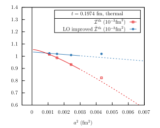
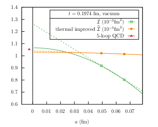
Figure 5: Left: Continuum limit for the truncated fourth moment of the thermal correlator, $I^{\rm th}(t=0.1974{\rm\,fm})$. The open symbols represent the uncorrected observable, the corresponding curve showing the (Q+log) fit to the data points at the three finest lattice spacings. The filled symbols, the three leftmost of which are fitted linearly in $a^{2}$, represent the leading-order improved observable. Right: Continuum limit for the truncated fourth moment of the vacuum correlator, $I(t=0.1974{\rm\,fm})$. The open symbols represent the straightforward estimator ${\cal I}(t,a)$, while the filled ones represent the estimator $\widehat{\cal I}(t,a)$ of Eq. (11). Both data sets are fitted linearly either in $a$ or in $a^{2}$. We also estimated the observable $I(t)$ using the perturbative five-loop vacuum spectral function, following Refs. Burnier and Laine (2012); Baikov et al. (2008), depicted with the red point.

The continuum estimate from the leading-order improved extrapolation is used to define the improved estimator of Eq. (11), which is shown in the right panel of Figure 5. The original data are displayed as open symbols; they exhibit a large cutoff effect. For illustration, two fit ansätze are employed, purely linear or purely quadratic in the lattice spacing. The latter may seem more plausible here, given the short-distance nature of the observable. Nevertheless, the severity of the cutoff effect leads to an unsatisfactory control of the continuum limit using only vacuum correlators with the available state-of-the-art lattice spacings. On the other hand, the thermal-improved estimator depicted with filled symbols shows an almost flat continuum limit, which suggests the subtraction of the thermal contribution also removes a significant amount of the cutoff effects, as expected. In this case, the continuum result is much less sensitive to the choice of fit ansatz for taking the continuum limit.

In order to quote a continuum estimate for the thermal-improved observable for illustration, we choose to use the continuum estimate of the thermal observable obtained with the LO-improvement, and for the correction the mean of the continuum estimates obtained with the linear and quadratic fits to arrive at

$$I(t) =1.035(9)_{\mathrm{stat}}(19)_{\mathrm{cont}}\times 10^{-3}\;\mathrm{fm}^{2},\qquad\quad t=0.1974\,\mathrm{fm}.$$ (40)

The second, systematic error associated with taking the continuum limit is estimated as the quadrature sum of (a) the difference between the (Q+log) extrapolation of ${\cal I}^{\rm th}$ and the (Q) extrapolation of $\mathring{\cal I}^{\rm th}$, and (b) half the difference between the linear and quadratic continuum fits of the correction term.

Finally, we compute the same observable in $N_{\mathrm{f}}=2$ massless perturbation theory based on the spectral representation Bernecker and Meyer (2011)

$$I(t)=\int_{2m_{\pi}}^{\infty}\mathrm{d}\omega\,\omega^{2}\,\rho(\omega^{2})\,\frac{\mathrm{d}^{4}}{\mathrm{d}\omega^{4}}\left(\frac{1-e^{-\omega t}}{\omega}\right),$$ (41)

where $\rho(\omega^{2})$ is the five-loop massless vacuum spectral function Burnier and Laine (2012); Baikov et al. (2008). We use the renormalization scale $\mu=2.4$ GeV and take $\Lambda_{\overline{\rm MS}}^{(2)}$ from the FLAG report Aoki et al. (2020). The result obtained is $I_{\mathrm{pert}}(t=0.1974\mathrm{fm})=1.059(-6)(1)\times 10^{-3}\mathrm{fm}^{2}$, which is depicted with the filled red point to the left in Figure 5. The errors are estimated using the uncertainty in $\Lambda_{\overline{\rm MS}}^{(2)}$. We find reasonable agreement between our final estimate and perturbation theory, even though we have not investigated the systematic effects associated with finite quark masses and residual non-perturbative effects, which might become relevant at the quoted level of precision. Also, we have not included the scale-setting uncertainty in Eq. (40); the relative scale-setting uncertainty of $I(t)$ is mainly that of $t^{2}/{\rm fm}^{2}$, i.e. about 2%, whereas $I(t)/t^{2}$ only depends weakly on $t$ around $t=0.2\,$fm.

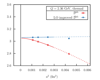
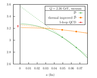
Figure 6: Continuum limit for the ‘thermal’ Adler function $D^{\rm th}(Q^{2})$ (left) and the corresponding vacuum observable $D(Q^{2})$ (right) for a large virtuality $Q=2.36$ GeV. The various data symbols and curves are entirely analogous to those in figure 5.

IV.2 The Adler function at large $Q^{2}$

The continuum limit of the thermal Adler function for a large value of the virtuality $Q=3\pi T=2.36$ GeV is shown in Figure 6. As in the previous case, the leading-order improved observable shows better scaling to the continuum limit, when the coarsest lattice spacing is not included. The original and thermal-improved estimator are shown in the right-hand panel of Figure 6, which likewise strongly suggests the suppression of lattice artifacts in the difference. Once again, the difficulty of performing a controlled continuum limit purely based on the vacuum correlators at large virtualities is apparent even with fine lattice spacings available. For illustration, we quote an estimate for the improved observable where the central value and systematic error are determined in the same way as in the subsection before

$$D(Q^{2}) =3.24(4)_{\mathrm{stat}}(3)_{\mathrm{cont}},\qquad\qquad Q=2.36\,{\rm GeV}.$$ (42)

For the five-loop perturbative result, using

$$D(Q^{2})=12\pi^{2}\,Q^{2}\int_{4m_{\pi}^{2}}^{\infty}\mathrm{d}\omega^{2}\,\frac{\rho(\omega^{2})}{(\omega^{2}+Q^{2})^{2}}$$ (43)

and the renormalization scale $\mu=Q$, we found $D_{\mathrm{pert}}(Q^{2})=3.24(-3)(1)$. Clearly, the perturbative prediction is in good agreement with our non-perturbative estimate obtained with the help of thermal correlators computed at very fine lattice spacings.

V Summary and outlook

We have shown that a better control over the continuum limit for short-distance dominated integrals over the vector correlator can be achieved by using thermal screening correlators at particularly fine lattice spacings, and then correcting for the difference. For the Adler function at a momentum $Q=2.36$  GeV, we estimate that we achieved a reduction of the systematic error due to the continuum limit by a factor of four, relative to the continuum limit based on the available vacuum correlators only. This is significant, since taking the continuum limit is responsible for one of the leading systematic errors on this quantity. The cost of generating the thermal ensembles at small lattice spacings is modest in comparison to the cost of the vacuum ensembles. The method can also be applied to the charm contribution, which is even more short-range and therefore more susceptible to large cutoff effects.

For the anomalous magnetic moment of the muon, we find that, in the time-momentum representation, performing a ‘naive’ linear extrapolation of the $t\leq 0.2$ fm contribution using lattice spacings down to 0.049 fm leads to an overestimate of about three percent as compared to our best estimate based on lattice spacings down to 0.033 fm. Since the muon $(g-2)$ is an observable which is much more infrared-weighted, the slightly inaccurate continuum extrapolation of the short-distance contribution in the $(u,d,s)$ quark sector only amounts to a difference of about $0.4\times 10^{-10}$ on this quantity, which is an order of magnitude smaller than the precision of the current most precise estimates Aoyama et al. (2020); Borsanyi et al. (2021). Nevertheless, we have seen clear evidence that performing additively tree-level improvement reduces the lattice artifacts in this short-distance regime and we thus recommend its use in future calculations of the leading hadronic contribution to $(g-2)_{\mu}$.

One may wonder, is it possible to calculate the hadronic contribution to the running of the QED coupling up to the $Z$-boson mass in lattice QCD with controlled errors? The methods and tests presented in this paper strongly suggest that it is indeed possible, and we now sketch a promising strategy. Let $\Delta_{2}\Pi(Q)\equiv\Pi(Q^{2})-\Pi(Q^{2}/4)$ be the difference of vacuum polarisations corresponding to the running of $\alpha$ over the momentum interval $Q/2$ to $Q$. Such an observable is very similar to the Adler function $D(Q^{2})$, in that it is dominated by Euclidean distances of order $1/Q$. What we have seen above leads us to conclude that $\Delta_{2}\Pi(Q^{2})$ for a large $Q\gg 1$ GeV can be computed at the one-percent level at a temperature $T\approx Q/(8\pi)$ in terms of the screening vector correlator; we may write this quantity $\Delta_{2}^{\rm th}\Pi(Q;T)$. The difference $\Delta_{2}^{\rm th}\Pi(Q;T/2)-\Delta_{2}^{\rm th}\Pi(Q;T)$ can be evaluated by performing simulations at temperatures differing by a factor of two with common lattice spacing. See Appendix E for an encouraging study at leading order in perturbation theory. Parametrically, the difference between $\Delta_{2}\Pi(Q)$ and $\Delta_{2}^{\rm th}\Pi(Q;T)$ is of order $(\pi T/Q)^{4}$, and thus $\Delta_{2}^{\rm th}\Pi(Q;T/2)-\Delta_{2}^{\rm th}\Pi(Q;T)$ already provides a sufficiently good estimate for that difference. The latter can also be estimated using perturbation theory, since a high value of $Q$ is tied to a high value of $T$. Thus by varying the temperature by factors of two, we can map out the running of $\alpha$ by factors of two in $Q$ up to the $Z$-boson mass. Such a program can be carried out on existing computing platforms, albeit at a significant investment, since realizing the double hierarchy $\pi T\ll Q\ll\pi/a$ typically requires the use of lattices of size $48\times 192^{3}$. If one resorts to such fine lattices, it is probably mandatory to address the freezing of the topological charge, for instance by using open boundary conditions in the $x_{3}$-direction Lüscher and Schaefer (2011); Florio et al. (2019).

Appendix A Derivation of the OPE for the vector correlator

In this appendix we use the operator-product expansion (OPE) as a tool to study the static screening correlator at short distance. To leading order in the expansion, the vacuum and thermal correlation functions are identical. The following term, linear in the distance $\absolutevalue{x_{3}}$, is in general non-vanishing for the thermal correlator. Here we ask ourselves if a suitable linear combination can be made such that this contribution cancels out. We will show that this is the case for the sum $G^{\mathrm{th}}_{00}(x_{3})+G^{\mathrm{th}}_{11}(x_{3})$. However, this does not necessarily lead to a better agreement between the vacuum and thermal correlation functions at short distance, due to the presence of constant terms which are not captured in the OPE picture. This point will be illustrated in the following.

As we discussed in some detail the OPE-based expansion of the electromagnetic-current correlator in a recent publication (Cè et al. (2021)), we largely refer to that for setting the notation and for the introduction of the main observables. More specifically, we make reference to the first few paragraphs of Section 3 for the definition of the Wilson coefficients and of the tower of local twist-two operators, and to the beginning of Section 3.1 for the operator mixing in the dimension-four sector. Moreover, we refer to Appendix B for the operator expectation values in the theory of free quarks.

A.1 Leading-order Wilson coefficients

We start by considering the expansion of the electromagnetic-current correlator in momentum space

$$\begin{split}i\int\mathrm{d}^{4}x\>e^{iq\cdot x}\>\langle{\rm T}\{J^{\mathrm{em}}_{\mu}(x)J^{\mathrm{em}}_{\nu}(0)\}\rangle\overset{\mathrm{LO}}{\sim}\sum_{n=2,4,\dots}\sum_{f}c_{f;\mu\nu\mu_{1}\dots\mu_{n}}(q)\>\langle O_{nf}^{\mu_{1}\dots\mu_{n}}\rangle\>.\end{split}$$ (44)

To leading order in the gauge coupling, only the fermionic operators $O_{nf}^{\mu_{1}\dots\mu_{n}}$ (Eq. (3.2) in Ref. Cè et al. (2021)) contribute, and they are accompanied by the Wilson coefficients

$$\begin{split}c_{f;\mu\nu\mu_{1}\dots\mu_{n}}(q)=&2Q_{f}^{2}\bigl{(}-g_{\mu\nu}+\frac{q_{\mu}q_{\nu}}{q^{2}}\bigr{)}2^{n}\frac{q_{\mu_{1}}\dots q_{\mu_{n}}}{(Q^{2})^{n}}\>+\\ &2Q_{f}^{2}\bigl{(}g_{\mu\mu_{1}}-\frac{q_{\mu}q_{\mu_{1}}}{q^{2}}\bigr{)}\bigl{(}g_{\nu\mu_{2}}-\frac{q_{\nu}q_{\mu_{2}}}{q^{2}}\bigr{)}2^{n}\frac{q_{\mu_{3}}\dots q_{\mu_{n}}}{(Q^{2})^{n-1}}\>,\end{split}$$ (45)

where $Q_{f}$ is the electric charge of the quark flavor $f$ and $Q^{2}=-q^{2}$. The contribution of the dimension-four operator with flavor $f$ is of the form

$$c_{f;\mu\nu\mu_{1}\mu_{2}}(q)\langle O_{2f}^{\mu_{1}\mu_{2}}\rangle\>,$$ (46)

where

$$O_{2f}^{\mu_{1}\mu_{2}}=\frac{i}{4}\,\Big{(}\bar{\psi}_{f}\gamma^{\{\mu_{1}}\overleftrightarrow{D}^{\mu_{2}\}}\psi_{f}-\frac{1}{4}g^{\mu_{1}\mu_{2}}\bar{\psi}_{f}\overleftrightarrow{D}\!\!\!\!\!/\;\psi_{f}\Big{)}\>.$$ (47)

Focusing now on the thermal correlation function, we express the tensor structure of the operator expectation value as in Ref. Cè et al. (2021)

$$\langle O_{2f}^{\mu_{1}\mu_{2}}\rangle_{T}=T^{2}\biggl{[}u^{\mu_{1}}u^{\mu_{2}}-\frac{1}{4}g^{\mu_{1}\mu_{2}}\biggr{]}\langle O_{2f}\rangle_{T}\>,$$ (48)

where $u$ is the four-velocity of the thermal medium. We fix $q_{0}=q_{1}=q_{2}=0$, as appropriate for the static screening correlator, and we choose the reference frame in which the thermal medium is at rest by setting $u=(1,\bm{0})$. Concentrating on the choices of indices $\mu=\nu=0,1$, we obtain

$$c_{f;00\mu_{1}\mu_{2}}(0,0,0,q_{3})\langle O_{2f}^{\mu_{1}\mu_{2}}\rangle_{T}=c_{f;11\mu_{1}\mu_{2}}(0,0,0,q_{3})\langle O_{2f}^{\mu_{1}\mu_{2}}\rangle_{T}=\frac{4Q_{f}^{2}T^{2}}{q_{3}^{2}}\langle O_{2f}\rangle_{T}\>.$$ (49)

Fourier-transforming with respect to the variable $q_{3}$ by using Eq. (B1) in Ref. Chetyrkin and Maier (2011), whose infrared regularization results in the $q_{3}$-independent term being zero,

$$\int_{-\infty}^{\infty}\frac{\mathrm{d}q_{3}}{2\pi}\>\frac{e^{-iq_{3}x_{3}}}{q_{3}^{2}}=\frac{\Gamma(-1/2)}{\sqrt{4\pi}\>\Gamma(1)}\biggl{(}\frac{x_{3}^{2}}{4}\biggr{)}^{1/2}=-\frac{\absolutevalue{x_{3}}}{2}\>,$$ (50)

we find for the coordinate-space version of Eq. (49)

$$\sum_{f}c_{f;00\mu_{1}\mu_{2}}(x_{3})\langle O_{2f}^{\mu_{1}\mu_{2}}\rangle_{T}=\sum_{f}c_{f;11\mu_{1}\mu_{2}}(x_{3})\langle O_{2f}^{\mu_{1}\mu_{2}}\rangle_{T}=-2\absolutevalue{x_{3}}\bigl{(}\sum_{f}Q_{f}^{2}\bigr{)}T^{2}\langle O_{2f}\rangle_{T}\>.$$ (51)

Finally, to get to the isovector vector-current correlators in Euclidean space-time we drop the factor $\sum_{f}Q_{f}^{2}$ and multiply by $-1$ the contribution to the correlator with two spatial indices. We obtain the OPE prediction to leading order in the gauge coupling

$$G^{\mathrm{th}}_{00}(x_{3})\overset{x_{3}\to 0}{\sim}G_{00}(x_{3})-2\absolutevalue{x_{3}}T^{2}\langle O_{2f}\rangle_{T}+O(\absolutevalue{x_{3}}^{3})$$ (52)

$$G^{\mathrm{th}}_{11}(x_{3})\overset{x_{3}\to 0}{\sim}G_{11}(x_{3})+2\absolutevalue{x_{3}}T^{2}\langle O_{2f}\rangle_{T}+O(\absolutevalue{x_{3}}^{3})\>.$$ (53)

In Appendix B we verify the correctness of the $O(\absolutevalue{x_{3}})$ term in the theory of free quarks. We observe that the term linear in $\absolutevalue{x_{3}}$ cancels out in the sum $G^{\mathrm{th}}_{00}(x_{3})+G^{\mathrm{th}}_{11}(x_{3})$. This fact is not sufficient to conclude that taking this combination improves the short-distance agreement with the vacuum correlation function $G_{00}(x_{3})=G_{11}(x_{3})$, because the OPE is not able to capture constant terms in the small-$x_{3}$ expansion, as those are not of short-distance origin. The free-theory correlators provide a concrete example of this situation, as shown in Figure 7. The figure shows the difference between the thermal correlation functions $G^{\mathrm{th}}_{00}(x_{3})$, $G^{\mathrm{th}}_{11}(x_{3})$ and their vacuum counterparts as a function of $x_{3}$, between $x_{3}=0$ and $x_{3}\simeq 0.4/T$. The leading OPE term, as explicitly computed in Appendix B, is also reported. Contrary to the OPE prediction, the difference between the thermal and vacuum correlators starts from a nonzero value in $x_{3}=0$. However, once we subtract $\Delta G_{0}\equiv[G^{\mathrm{th}}-G]_{x_{3}=0}$, we find that the truncated OPE provides indeed a good description of $(G^{\mathrm{th}}-G-\Delta G_{0})$ at small $x_{3}$.

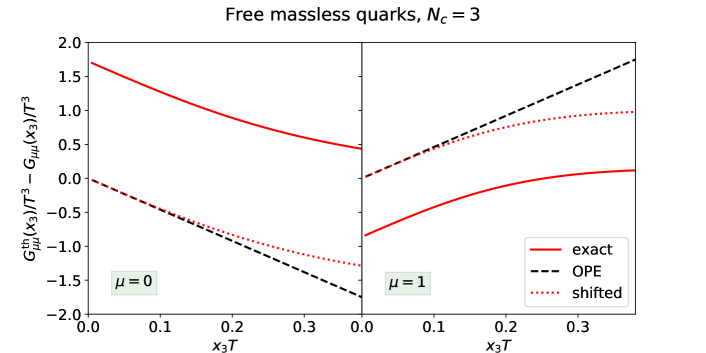
Figure 7: Difference between the thermal and vacuum correlation functions $G^{\mathrm{th}}_{\mu\mu}(x_{3})-G_{\mu\mu}(x_{3})$ for $\mu=0$ (left) and $\mu=1$ (right) at small $x_{3}$ in the free theory. The black dashed line represents the OPE prediction for this quantity truncated at leading order in $x_{3}$, and the red dotted line is obtained by subtracting $[G^{\mathrm{th}}_{\mu\mu}-G_{\mu\mu}]_{x_{3}=0}$ from the red curve.

A.2 Next-to-leading-order Wilson coefficients

To higher order in perturbation theory, the mixing under renormalization with the gluonic twist-two operators $O_{ng}^{\mu_{1}\dots\mu_{n}}$ (Eq. (3.3) in Ref. Cè et al. (2021)) must be taken into account. To write explicitly the contribution from the dimension-four operators to NLO precision, we follow closely the sections 3 and 3.1 of Ref. Cè et al. (2021) and refer to those for any unexplained notation. Going back to Eq. (49), its NLO equivalent is obtained by making the substitution

$$\begin{split}\langle O_{2f}\rangle_{T}\>\longrightarrow\>&\frac{1}{2}\frac{1}{16/3+N_{f}}\frac{e+p}{T^{2}}+\\ &\frac{1}{N_{f}(16/3+N_{f})}\biggl{(}\frac{\log(q_{3}^{2}/\Lambda^{2})}{\log(\tilde{\mu}^{2}/\Lambda^{2})}\biggr{)}^{\gamma}\biggl{(}\frac{16}{3}\sum_{f^{\prime}}\langle O_{2f^{\prime}}\rangle_{T}-N_{f}\langle O_{2g}\rangle_{T}\biggl{)}\>,\end{split}$$ (54)

where $e$ and $p$ are the energy density and the pressure of the thermal medium and $\tilde{\mu}$ and $\Lambda$ represent two energy scales, respectively the one at which the local operators are renormalized and the one at which the one-loop renormalized coupling diverges. The power $\gamma$ is one of the eigenvalues of the anomalous-dimension matrix,

$$\gamma=-\frac{4}{3}\biggl{(}\frac{16}{3}+N_{f}\biggr{)}\frac{1}{2b_{0}}\overset{N_{f}=2}{=}-0.51\>,$$ (55)

where $b_{0}=11-\frac{2}{3}N_{f}$ is the coefficient of the one-loop contribution to the beta function.

To get the final expression in position space, we are faced with the problem of computing the Fourier transform

$$\frac{1}{2\pi}\int_{-\infty}^{\infty}\mathrm{d}q_{3}\>e^{-iq_{3}x_{3}}\>\frac{\log(q_{3}^{2}/\Lambda^{2})^{\gamma}}{q_{3}^{2}}\>.$$ (56)

As in the case of Eq. (50), the Fourier integral is divergent and a regularization procedure is needed to correctly extract the asymptotic dependence on $x_{3}$. We discuss this point in detail in Appendix C and report here the final result

$$\frac{\log(q_{3}^{2}/\Lambda^{2})^{\gamma}}{q_{3}^{2}}\>\overset{\mathrm{coord.\>\>space}}{\longrightarrow}\>-\frac{\absolutevalue{x_{3}}}{2}\log(1/(x_{3}\Lambda)^{2})^{\gamma}\>.$$ (57)

The OPE prediction to NLO in the gauge coupling reads

$$\begin{split}G^{\mathrm{th}}_{\mu\mu}(x_{3})-G_{\mu\mu}(x_{3})\overset{\mathrm{NLO}}{\sim}&s_{\mu}2\absolutevalue{x_{3}}T^{2}\biggl{\{}\frac{1}{2}\frac{1}{16/3+N_{f}}\frac{e+p}{T^{2}}+\\ &\frac{1}{N_{f}(16/3+N_{f})}\biggl{(}\frac{\log(1/(x_{3}\Lambda)^{2})}{\log(\tilde{\mu}^{2}/\Lambda^{2})}\biggr{)}^{\gamma}\biggl{(}\frac{16}{3}\sum_{f^{\prime}}\langle O_{2f^{\prime}}\rangle_{T}-N_{f}\langle O_{2g}\rangle_{T}\biggl{)}\biggr{\}}+O(\absolutevalue{x_{3}}^{3})\>,\end{split}$$ (58)

where $\mu\neq 3$ and $s_{\mu}$ is a sign factor evaluating to 1 for $\mu=1,2$ and to $-1$ for $\mu=0$. While we did not discuss explicitly the case $\mu=2$ so far, we point out that the symmetries of the screening correlator constrain it to be equal to the case $\mu=1$. In the extreme $x_{3}\to 0$ limit the logarithmic contribution is subleading, and we find

$$\bigl{[}G^{\mathrm{th}}_{\mu\mu}(x_{3})-G_{\mu\mu}(x_{3})\bigr{]}_{\mathrm{NLO}}\overset{x_{3}\to 0}{\sim}s_{\mu}\absolutevalue{x_{3}}\frac{e+p}{16/3+N_{f}}\>,\quad\mu\neq 3\>.$$ (59)

As already pointed out in Ref. Cè et al. (2021) relative to the structure functions of the quark-gluon plasma, the free-theory prediction of Eqs. (52), (53) is not recovered in the short-distance limit $x_{3}\to 0$, contrary to the intuition coming from the property of asymptotic freedom. As a consequence of the mixing between operators under renormalization, the free theory represents here an extreme case which is not connected to the real interacting theory by an expansion in powers of the QCD coupling.

Appendix B Test of the leading OPE prediction in the free theory

The expressions (52), (53) can be verified in the theory of free quarks. In this case, the expectation value of the dimension-four operator reads (see Appendix B of Ref. Cè et al. (2021))

$$\langle O_{2f}\rangle^{\mathrm{free}}_{T}=\frac{7\pi^{2}T^{2}N_{c}}{90}\>,$$ (60)

where $N_{c}$ is the number of colors. We can verify the OPE prediction by expanding the free correlation function in powers of $\absolutevalue{x_{3}}$. To do this, we make use of Eqs. (3.5) and (3.6) in Ref. Brandt et al. (2014), which give the free thermal vector correlator projected to Matsubara frequency $k_{n}$ as a function of the spatial coordinates $\bm{r}=(x_{1},x_{2},x_{3})$. After identifying the relevant terms in the expansion in powers of $\bm{r}$, we project to zero momentum in the directions $x_{1}$ and $x_{2}$ to obtain the corresponding contribution to the screening correlator. In the static sector $k_{n}=0$, we have

$$G_{00}^{(k_{n}=0)}(\bm{r})=-\frac{N_{c}T^{3}}{r^{2}}\biggl{(}\frac{\cosh\bar{r}}{\bar{r}\sinh^{2}\bar{r}}+\frac{1}{{\bar{r}}^{2}\sinh\bar{r}}\biggr{)}\>,$$ (61)

and

$$\begin{split}G_{11}^{(k_{n}=0)}(\bm{r})=\frac{N_{c}T^{3}}{r^{2}}\biggr{\{}&\frac{x_{1}^{2}}{r^{2}}\biggr{[}\frac{\cosh\bar{r}}{\bar{r}\sinh^{2}\bar{r}}+\frac{1}{{\bar{r}}^{2}\sinh\bar{r}}\biggr{]}\\ &-\biggl{(}1-\frac{x_{1}^{2}}{r^{2}}\biggr{)}\biggl{[}\frac{\cosh\bar{r}}{\bar{r}\sinh^{2}\bar{r}}+\frac{1}{{\bar{r}}^{2}\sinh\bar{r}}+\frac{1}{2\sinh\bar{r}}+\frac{1}{\sinh^{3}\bar{r}}\biggr{]}\biggr{\}}\>,\end{split}$$ (62)

where $\bar{r}\equiv 2\pi Tr$ and $r\equiv\absolutevalue{\bm{r}}$. We start by expanding Eq. (61) in powers of the spatial coordinates. In the OPE picture, we expect a contribution from the dimension-four operator of the form

$$\frac{\tilde{c}_{\mu_{1}\mu_{2}}\langle O_{2f}^{\mu_{1}\mu_{2}}\rangle}{r}\>,$$ (63)

where $\tilde{c}_{\mu_{1}\mu_{2}}$ is a dimensionless coefficient. Therefore we are interested in the term proportional to $1/r$ in the expansion

$$G_{00}^{(k_{n}=0)}(\bm{r})=-\frac{N_{c}T^{4}}{r}\>\frac{2\pi}{{\bar{r}}^{4}}\biggl{(}2-\frac{7}{180}{\bar{r}}^{4}+O({\bar{r}}^{6})\biggr{)}\>,$$ (64)

which is

$$\frac{7\pi N_{c}T^{4}}{90}\frac{1}{r}\>.$$ (65)

To project to zero momentum in the directions $x_{1}$ and $x_{2}$, we make use of the following equation

$$\begin{split}\int_{-\infty}^{\infty}\frac{\mathrm{d}x_{1}\mathrm{d}x_{2}}{r}&=2\pi\lim_{L\to\infty}\int_{0}^{L}\frac{\rho\>\mathrm{d}\rho}{\sqrt{\rho^{2}+x_{3}^{2}}}=2\pi\lim_{L\to\infty}\bigl{(}-\absolutevalue{x_{3}}+\sqrt{L^{2}+x_{3}^{2}}\bigr{)}\\ &=-2\pi\absolutevalue{x_{3}}+\mathrm{proportional\>to\>spatial\>extent,\>independent\>of\>}x_{3}\>.\end{split}$$ (66)

To conclude, the linear term in the expansion of the correlator $G^{\mathrm{th}}_{00}(x_{3})$ in powers of $\absolutevalue{x_{3}}$ is given by

$$-\frac{7\pi^{2}N_{c}T^{4}}{45}\absolutevalue{x_{3}}\>,$$ (67)

and it is in agreement with the OPE prediction $-2\absolutevalue{x_{3}}T^{2}\langle O_{2f}\rangle_{T}^{\mathrm{free}}$.

We now repeat the same procedure for the correlator (62). In this case, the contribution from the dimension-four operator is of the form

$$\biggl{(}\frac{\tilde{c}_{\mu_{1}\mu_{2}}}{r}+\frac{x_{1}^{2}}{r^{3}}\tilde{d}_{\mu_{1}\mu_{2}}\biggr{)}\langle O_{2f}^{\mu_{1}\mu_{2}}\rangle\>,$$ (68)

where $\tilde{c}_{\mu_{1}\mu_{2}}$ and $\tilde{d}_{\mu_{1}\mu_{2}}$ are dimensionless coefficients. From the expansion

$$\begin{split}G_{11}^{(k_{n}=0)}(\bm{r})=N_{c}T^{3}\biggr{\{}&\frac{x_{1}^{2}}{r^{3}}\>\frac{2\pi T}{{\bar{r}}^{4}}\biggr{[}2-\frac{7}{180}{\bar{r}}^{4}+O({\bar{r}}^{6})\biggr{]}\\ &-\biggl{(}\frac{1}{r}-\frac{x_{1}^{2}}{r^{3}}\biggr{)}\frac{2\pi T}{{\bar{r}}^{4}}\biggl{[}3+\frac{7}{360}{\bar{r}}^{4}+O({\bar{r}}^{6})\biggr{]}\biggr{\}}\>,\end{split}$$ (69)

we see that the terms proportional to $1/r$ and $x_{1}^{2}/r^{3}$ are given by

$$-\frac{7\pi N_{c}T^{4}}{180}\biggl{(}\frac{1}{r}+\frac{x_{1}^{2}}{r^{3}}\biggr{)}\>.$$ (70)

We project to zero momentum in the directions $x_{1}$ and $x_{2}$ by applying the following procedure

$$\begin{split}\int_{-\infty}^{\infty}\mathrm{d}x_{1}\mathrm{d}x_{2}\>\biggl{(}\frac{1}{r}+\frac{x_{1}^{2}}{r^{3}}\biggr{)}&=2\pi\lim_{L\to\infty}\biggl{(}\int_{0}^{L}\mathrm{d}\rho\frac{\rho}{\sqrt{\rho^{2}+x_{3}^{2}}}+\frac{1}{2}\int_{0}^{L}\mathrm{d}\rho\frac{\rho^{3}}{(\rho^{2}+x_{3}^{2})^{\frac{3}{2}}}\biggr{)}\\ &=2\pi\lim_{L\to\infty}\biggl{(}-\absolutevalue{x_{3}}+\sqrt{L^{2}+x_{3}^{2}}+\frac{1}{2}\frac{L^{2}+2x_{3}^{2}-2\absolutevalue{x_{3}}\sqrt{L^{2}+x_{3}^{2}}}{\sqrt{L^{2}+x_{3}^{2}}}\biggr{)}\\ &=-4\pi\absolutevalue{x_{3}}+\mathrm{proportional\>to\>spatial\>extent,\>independent\>of\>}x_{3}\>.\end{split}$$ (71)

To conclude, the linear term in the expansion of $G^{\mathrm{th}}_{11}(x_{3})$ in powers of $\absolutevalue{x_{3}}$ is

$$\frac{7\pi^{2}N_{c}T^{4}}{45}\absolutevalue{x_{3}}$$ (72)

and it agrees with the OPE prediction $2\absolutevalue{x_{3}}T^{2}\langle O_{2f}\rangle_{T}^{\mathrm{free}}$.

Appendix C Fourier transform of $\log(q^{2}/\Lambda^{2})^{\gamma}/q^{2}$

The authors of Ref. Wong and Lin (1978) study the the asymptotic behaviour for $q\to\infty$ of the one-sided Fourier transform

$$F(q)=\int_{0}^{\infty}\differential{x}e^{iqx}f(x)$$ (73)

of a function that has logarithmic singularities for $x\to 0^{+}$

$$f(x)\sim\sum_{m=0}^{\infty}c_{m}x^{\alpha_{m}-1}(-\log x)^{\beta_{m}},$$ (74)

where $\alpha_{m}\to+\infty$ as $m\to\infty$ with $\real\alpha_{m+1}\geq\real\alpha_{m}$, and the $\beta_{m}$ are arbitrary complex numbers. The main result is that for $q\to\infty$ holds

$$F(q)=\sum_{m=0}^{M-1}c_{m}J(\alpha_{m},\beta_{m},q)+o(q^{-n})$$ (75)

where $M$ is a positive integer such that $\real\alpha_{M-1}\leq n<\real\alpha_{M}$ and

$$J(\alpha,\beta,q)=\int_{0}^{\infty e^{i\theta}}\differential{x}e^{iqx}x^{\alpha-1}(-\log x)^{\beta}\sim\frac{e^{\alpha\pi i/2}}{q^{\alpha}}\sum_{r=0}^{\infty}c_{r}(\alpha,\beta)(\log q)^{\beta-r},$$ (76)

with the $c_{r}(\alpha,\beta)$ given by

$$c_{r}(\alpha,\beta)=(-1)^{r}{\beta\choose r}\sum_{k=0}^{r}{r\choose k}\Gamma^{(k)}(\alpha)\left(\frac{\pi i}{2}\right)^{r-k}.$$ (77)

Setting $M=1$, $\alpha_{0}=2$ and $\beta_{0}=\gamma$, and using $c_{0}(2,\gamma)=1$ we obtain

$$f(x)\stackrel{{\scriptstyle x\to 0^{+}}}{{\sim}}x(-\log x)^{\gamma}\quad\Rightarrow\quad F(q)\stackrel{{\scriptstyle q\to\infty}}{{\sim}}-\frac{(\log q)^{\gamma}}{q^{2}}\left[1+\sum_{r=1}^{\infty}c_{r}(2,\gamma)(\log q)^{-r}\right]+o(q^{-2}).$$ (78)

An arbitrary number of subleading $(\log q)^{r}$ terms in the asymptotic behaviour of $F(q)$ can be removed with appropriately chosen $\alpha_{m}$ and $\beta_{m}$. In particular, we found that setting $\alpha_{m}=\alpha$, $\beta_{m}=\gamma-m$ and

$$d_{m}(\alpha,\gamma)=(-1)^{r}{\gamma\choose m}\sum_{k=0}^{m}{m\choose k}\Gamma(\alpha)\derivative[k]{\alpha}\frac{1}{\Gamma(\alpha)}\left(\frac{\pi}{2i}\right)^{m-k}$$ (79)

we obtain

$$f(x)\stackrel{{\scriptstyle x\to 0^{+}}}{{\sim}}\sum_{m=0}^{\infty}d_{m}(\alpha,\gamma)x^{\alpha-1}(-\log x)^{\gamma-m}\quad\Rightarrow\quad F(q)\stackrel{{\scriptstyle q\to\infty}}{{\sim}}\frac{e^{\alpha\pi i/2}}{q^{\alpha}}(\log q)^{\gamma}+o(q^{-\alpha}),$$ (80)

or, in the $\alpha=2$ case,

$$f(x)\stackrel{{\scriptstyle x\to 0^{+}}}{{\sim}}\sum_{m=0}^{\infty}d_{m}(2,\gamma)x(-\log x)^{\gamma-m}\quad\Rightarrow\quad F(q)\stackrel{{\scriptstyle q\to\infty}}{{\sim}}-\frac{(\log q)^{\gamma}}{q^{2}}+o(q^{-2}).$$ (81)

From this it is easy to show that for $\gamma\in\mathbb{R}$ a function with the asymptotic behaviour

$$\frac{(\log q^{2}/\Lambda^{2})^{\gamma}}{q^{2}}\qquad\text{for $q\to\infty$}$$ (82)

is the two-sided Fourier transform of a function that goes like

$$-\frac{\absolutevalue{x}}{2}\left(\log\frac{1}{(\absolutevalue{x}\Lambda)^{2}}\right)^{\gamma}\left[1+\sum_{m=1}^{\infty}\real d_{m}(2,\gamma)\left(\frac{1}{2}\log\frac{1}{(\absolutevalue{x}\Lambda)^{2}}\right)^{-m}\right]\qquad\text{for $x\to 0$}.$$ (83)

The first coefficients in the sum in the r.h.s. evaluates to

$$\real d_{1}(2,\gamma)=2(1-\gamma_{E})\gamma\approx$0.422\,784$\gamma,$$ (84)

$$\real d_{2}(2,\gamma)\approx$-1.466\,79$\gamma(\gamma-1),$$ (85)

$$\real d_{3}(2,\gamma)\approx$-0.712\,68$\gamma(\gamma-1)(\gamma-2),$$ (86)

$$\real d_{3}(2,\gamma)\approx$0.516\,685$\gamma(\gamma-1)(\gamma-2)(\gamma-3).$$ (87)

Appendix D Details on the lattice free-theory computation

In this appendix we collect some details on the free-theory computation. In the theory of non-interacting massless Wilson quarks, defined on a spatially-infinite lattice, the zero-temperature quark propagator can be expressed as

$$\begin{split}\langle\psi_{f}(x)\bar{\psi}_{f}(y)\rangle=&\int_{-\frac{\pi}{a}}^{\frac{\pi}{a}}\frac{\mathrm{d}^{3}p}{(2\pi)^{3}}\>\frac{e^{-\omega_{\bm{p}}\absolutevalue{x_{3}-y_{3}}+i\bm{p}\cdot(\bm{x}-\bm{y})}}{D(\bm{p})}\times\\ &\biggl{(}\mathrm{sgn}(x_{3}-y_{3})\frac{1}{a}\sinh(a\omega_{\bm{p}})\gamma_{3}-i\bm{\gamma}\cdot\mathring{\bm{p}}+C(\bm{p})+\delta_{x_{3},y_{3}}\frac{1}{a}\sinh(a\omega_{\bm{p}})\biggr{)}\>,\end{split}$$ (88)

where

$$\mathring{p}_{\mu}=\frac{1}{a}\sin(ap_{\mu})\>,\quad\hat{p}_{\mu}=\frac{2}{a}\sin\bigl(\frac{ap_{\mu}}{2}\bigr{missing})\>,$$ (89)

$$A(\bm{p})=1+\frac{1}{2}a^{2}\hat{\bm{p}}^{\>2}\>,\quad B(\bm{p})=\hat{\bm{p}}^{\>2}+\frac{1}{2}a^{2}\sum_{k<l}{\hat{p}}^{2}_{k}{\hat{p}}^{2}_{l}\>,\quad C(\bm{p})=\frac{a}{2}\biggl{(}\hat{\bm{p}}^{\>2}-\frac{B(\bm{p})}{A(\bm{p})}\biggr{)}\>,$$ (90)

$$D(\bm{p})=\sqrt{B(\bm{p})\bigl{(}4A(\bm{p})+a^{2}B(\bm{p})\bigr{)}}=\frac{2}{a}A(\bm{p})\sinh(a\omega_{\bm{p}})\>.$$ (91)

The sign function in Eq. (88) evaluates to zero when its argument is zero, and the vector $\bm{p}$ has three components denoted by $(p_{0},p_{1},p_{2})$. Similarly, $\bm{\gamma}=(\gamma_{0},\gamma_{1},\gamma_{2})$ and $\bm{x}=(x_{0},x_{1},x_{2})$. At finite temperature $T$, the thermal propagator $\langle\psi_{f}(x)\bar{\psi}_{f}(y)\rangle_{T}$ can be obtained from Eq. (88) by assigning to $p_{0}$ discrete values corresponding to the fermionic Matsubara frequencies $p_{0}=(2n+1)\pi T$, and by making the substitution

$$\int_{-\frac{\pi}{a}}^{\frac{\pi}{a}}\frac{\mathrm{d}p_{0}}{2\pi}\to T\sum_{n=0}^{N_{t}-1}\>,$$ (92)

where $N_{t}=1/(aT)$ is the number of lattice points in the Euclidean-time direction. With the propagators at hand, we have all the elements to compute the correlation functions (12) and (15) in the massless free theory. In the vacuum, and for $\mu=\nu\neq 3$, we have

$$\begin{split}\mathcal{G}_{\mu\mu}(x_{3})\overset{\mu\neq 3}{=}4N_{c}\int_{-\frac{\pi}{a}}^{\frac{\pi}{a}}\frac{\mathrm{d}^{3}p}{(2\pi)^{3}}\frac{e^{-2\omega_{\bm{p}}\absolutevalue{x_{3}}}}{D(\bm{p})^{2}}&\biggl{[}2\mathring{p}_{\mu}\sin(ap_{\mu})\bigl{(}C(\bm{p})+\delta_{x_{3},0}\frac{1}{a}\sinh(a\omega_{\bm{p}})\bigr{)}\\ &-\cos(ap_{\mu})\biggl{(}\mathrm{sgn}(x_{3})^{2}\frac{1}{a^{2}}\sinh^{2}(a\omega_{\bm{p}})-2{\mathring{p}_{\mu}}^{2}+\mathring{\bm{p}}^{2}\\ &+\bigl{(}C(\bm{p})+\delta_{x_{3},0}\frac{1}{a}\sinh(a\omega_{\bm{p}})\bigr{)}^{2}\biggr{)}\biggr{]}\>,\end{split}$$ (93)

where $N_{c}$ represents the number of colors. In the vacuum and in infinite volume there is no difference between projecting to zero momentum in the directions $(x_{1},x_{2},x_{3})$ or $(x_{0},x_{1},x_{2})$. In this appendix we choose the second option, in order to keep a closer analogy with the thermal screening correlator. The thermal correlation function $\mathcal{G}^{\mathrm{th}}_{\mu\mu}(x_{3})$, with $\mu\neq 3$, can be obtained starting from Eq. (93) and exchanging the integral over $p_{0}$ with a sum over fermionic Matsubara modes, as in Eq. (92).

We consider the fourth-moment observable $\mathcal{I}(t)$ as defined in Eq. (16). In the limit $a\to 0$ its integrand reads

$$\begin{split}x_{3}^{4}\>\mathcal{G}(x_{3})=x_{3}^{4}\int_{-\frac{\pi}{a}}^{\frac{\pi}{a}}\frac{\mathrm{d}^{3}p}{(2\pi)^{3}}\>e^{-2p\absolutevalue{x_{3}}}\biggl{[}\hat{f}_{0,0}(\hat{\bm{p}})\>+a^{2}\bigl{(}p^{2}\hat{f}_{2,0}(\hat{\bm{p}})+\absolutevalue{x_{3}}p^{3}\hat{f}_{2,1}(\hat{\bm{p}})\bigr{)}+O(a^{4})\biggr{]}\>,\end{split}$$ (94)

where

$$\hat{f}_{0,0}(\hat{\bm{p}})=2N_{c}\biggl{(}1-\frac{p_{1}^{2}}{p^{2}}\biggr{)}\>,$$ (95)

$$\hat{f}_{2,0}(\hat{\bm{p}})=-2N_{c}\biggl{[}1-\frac{1}{2}\frac{p_{1}^{2}}{p^{2}}\biggl{(}1-\frac{2}{3}\>\frac{p_{0}^{4}+p_{1}^{4}+p_{2}^{4}}{p^{4}}+\frac{5}{3}\>\frac{p_{1}^{2}}{p^{2}}\biggr{)}\biggr{]}\>,$$ (96)

$$\hat{f}_{2,1}(\hat{\bm{p}})=N_{c}\>\frac{2}{3}\biggl{(}1-\frac{p_{1}^{2}}{p^{2}}\biggr{)}\biggl{(}1+\frac{p_{0}^{4}+p_{1}^{4}+p_{2}^{4}}{p^{4}}\biggr{)}\>.$$ (97)

As before we have $\bm{p}=(p_{0},p_{1},p_{2})$, and we introduced the notation $p\equiv\absolutevalue{\bm{p}}$. We observe that a generic term of the expansion within square brackets in Eq. (94) can be expressed as

$$a^{n}\absolutevalue{x_{3}}^{m}p^{n+m}\hat{f}_{n,m}(\hat{\bm{p}})\>,$$ (98)

with $n=2,4,\dots$, $m\geq 0$ and where the dimensionless function $\hat{f}_{n,m}(\hat{\bm{p}})$ contains the dependence on the orientation of the vector $\bm{p}$ ($\hat{\bm{p}}\equiv\bm{p}/p$).

Appendix E Analysis of $\Delta_{2}\Pi(Q^{2})$ in the theory of free quarks

As an outlook towards future applications, a strategy to compute the hadronic contribution to the running of the electromagnetic coupling up to the $Z$ mass is outlined in Section V. In this appendix, we test the core of this strategy in the theory of massless free quarks, whose lattice formulation is described in detail in Section III.1 and in Appendix D. The observable under analysis is

$$\begin{split}\Delta_{2}\Pi(Q^{2})&\equiv\Pi(Q^{2})-\Pi(Q^{2}/4)\\ &=\int_{0}^{\infty}\mathrm{d}x_{3}G(x_{3})\frac{4}{Q^{2}}\biggl{[}4\sin^{2}\biggl{(}\frac{Qx_{3}}{4}\biggr{)}-\sin^{2}\biggl{(}\frac{Qx_{3}}{2}\biggl{)}\biggl{]}\>,\end{split}$$ (99)

where $\Pi(Q^{2})$ is the hadronic vacuum polarization and the correlation function $G(x_{3})$ is defined in Eq. (4). The thermal equivalents at two different temperatures $\Delta_{2}^{\mathrm{th}}\Pi(Q^{2};T)$, $\Delta_{2}^{\mathrm{th}}\Pi(Q^{2};T/2)$ are also considered. The temperature is fixed to $T=Q/(8\pi)$. In view of computing this observable on the lattice, an upper cut $x_{3}^{\mathrm{cut}}=2/T$ is set in the integral of Eq. (99). The lattice observables are denoted by $\Delta_{2}\mathbf{\Pi}(Q^{2})$, $\Delta_{2}^{\mathrm{th}}\mathbf{\Pi}(Q^{2};T)$. As in the analysis presented in Section III, we fix the physical value of the temperature to $T=246.25$ MeV, which is close to the temperature of the QCD ensembles considered in this study, and which assigns to the lattice Euclidean-time direction the physical extent $1/T=0.8$ fm. As a consequence, $Q=8\pi T\simeq 6.2$ GeV.

The first step consists in obtaining a continuum estimate of the thermal observable $\Delta_{2}\mathbf{\Pi}(Q^{2};T)$. With this goal, we consider four lattices with temperature $T$ and with $N_{t}=24,32,40,48$ lattice sites in the Euclidean-time direction. The temperature and the lattice spacing are related by $T=1/(aN_{t})$. With this setup, and making good use of the knowledge about the logarithmic lattice artifacts (see Section III.2), we obtain a continuum estimate differing from the correct continuum value by only $0.1\%$. The lattice data and the fit curves are shown in the left panel of Figure 8 together with the correct continuum value, the accuracy of the resulting continuum estimates is reported in Table 6. The prefactor of the $O(a^{2}\log(1/a))$ cutoff effect, which we denote by $\tilde{c}_{\Delta_{2}\mathbf{\Pi}}$, can be computed by observing that the short-distance limit of the integration kernel is

$$\frac{4}{Q^{2}}\biggl{[}4\sin^{2}\biggl{(}\frac{Qx_{3}}{4}\biggr{)}-\sin^{2}\biggl{(}\frac{Qx_{3}}{2}\biggl{)}\biggl{]}\overset{x_{3}\to 0}{\sim}\frac{Q^{2}}{16}x_{3}^{4}\>,$$ (100)

which implies

$$\tilde{c}_{\Delta_{2}\mathbf{\Pi}}=\frac{Q^{2}}{16}\tilde{c}_{\mathcal{I}}=\frac{7Q^{2}}{320\pi^{2}}\>.$$ (101)

The value of $\tilde{c}_{\mathcal{I}}$ is given in Eq. (28).

Table 6: Accuracy of the continuum extrapolation of the thermal quantity $\Delta_{2}^{\mathrm{th}}\mathbf{\Pi}(Q^{2};T)$, measured against the correct continuum value. The label “plain” refers to fitting the plain lattice observable, while for the case “subtr.” the logarithmic lattice artifact is subtracted as $\Delta_{2}^{\mathrm{th}}\mathbf{\Pi}(Q^{2};T)-\tilde{c}_{\Delta_{2}\mathbf{\Pi}}a^{2}\log(1/(Ta))$. For the choice of scales made here $T=246.25$ MeV, $Q=8\pi T\simeq 6.2$ GeV, we have $\tilde{c}_{\Delta_{2}\mathbf{\Pi}}\simeq 2.2\leavevmode\nobreak\ \mathrm{fm}^{-2}$ (see Eq. (101)). The lattice data and the fit curves are shown in Figure 8, left panel.

$\absolutevalue{c_{0}-\Delta_{2}^{\mathrm{th}}\Pi}/\Delta_{2}^{\mathrm{th}}\Pi\>\>\>$		$\tilde{c}\leavevmode\nobreak\ [\mathrm{fm}^{-2}]$	ansatz
0.8%	0.9%	–	$c_{0}+c_{2}a^{2}$
0.7%	0.1 %	–	$c_{0}+c_{2}a^{2}+c_{4}a^{4}$
0.6%	–	0.29	$c_{0}+a^{2}[c_{2}+\tilde{c}\log(1/(Ta))]$
0.1%	–	1.6	$c_{0}+a^{2}[c_{2}+\tilde{c}\log(1/(Ta))]+c_{4}a^{4}$
plain	subtr.

The difference between the thermal observable $\Delta_{2}^{\mathrm{th}}\Pi(Q^{2};T)$ and its vacuum counterpart is of about one percent. To correct for this bias, we add a continuum estimate of the difference $\Delta_{2}^{\mathrm{th}}\mathbf{\Pi}(Q^{2};T/2)-\Delta_{2}^{\mathrm{th}}\mathbf{\Pi}(Q^{2};T)$. Within the desired precision, this is a good-enough approximation of the difference between the vacuum observable and $\Delta_{2}^{\mathrm{th}}\Pi(Q^{2};T)$, and it has the advantage of being cheaper to compute at equal lattice spacing. Quantitatively, the continuum values $\Delta_{2}\Pi(Q^{2})$ and $\Delta_{2}^{\mathrm{th}}\Pi(Q^{2};T/2)$ differ by only one permille. We consider two lattices with temperature $T$ and $N_{t}=20,24$ points in the Euclidean-time direction and their equivalents with temperature $T/2$, same lattice spacing and double the points in the compact direction. Extrapolating linearly in $a^{2}$ we obtain a $0.2\%$-precise estimate of the continuum value $\Delta_{2}^{\mathrm{th}}\Pi(Q^{2};T/2)-\Delta_{2}^{\mathrm{th}}\Pi(Q^{2};T)$. Considering only the finest available lattice spacing, corresponding to $N_{t}=24$ for the lattice with temperature $T$ and $N_{t}^{(T/2)}=2N_{t}=48$ for the temperature-$T/2$ one, the difference between the lattice observable $\Delta_{2}^{\mathrm{th}}\mathbf{\Pi}(Q^{2};T/2)-\Delta_{2}^{\mathrm{th}}\mathbf{\Pi}(Q^{2};T)$ and its continuum value is of about $7\%$. The lattice data, the fit curve and the continuum value of the observable are shown in the right panel of Figure 8.

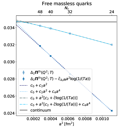
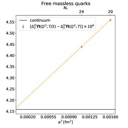
Figure 8: Left: continuum extrapolation of the thermal observable $\Delta_{2}^{\mathrm{th}}\mathbf{\Pi}(Q^{2};T)$, with $T=246.25$ MeV and $Q=8\pi T\simeq 6.2$ GeV. The $O(a^{2}\log(1/a))$ lattice artifact is either included in the fit ansatz or explicitly subtracted by using the known prefactor $\tilde{c}_{\Delta_{2}\mathbf{\Pi}}$ (101). The accuracy of the resulting continuum estimates is reported in Table 6. Right: continuum extrapolation of the bias correction $[\Delta_{2}^{\mathrm{th}}\mathbf{\Pi}(Q^{2};T/2)-\Delta_{2}^{\mathrm{th}}\mathbf{\Pi}(Q^{2};T)]$, together with its known continuum value. The fit ansatz is linear in $a^{2}$.

To conclude, the free-theory analysis indicates that the strategy outlined in Section V to compute the hadronic contribution to the running of $\alpha_{\mathrm{em}}$ up to large energy scales (compared to the hadronic scales easily accessible on the lattice) is feasible with the setup and lattice sizes suggested there. The idea is to study the difference of hadronic vacuum polarizations $\Delta_{2}\Pi(Q^{2})$ between the scales $Q$ and $Q/2$ making use of thermal lattices with temperatures $T\approx Q/(8\pi)$ and $T/2$. Having fixed $T=246.25$ MeV and $Q=8\pi T\simeq 6.2$ GeV, and having considered lattices with at the most 48 points in the Euclidean-time direction, we obtained a $0.1\%$-precise estimate of the thermal quantity $\Delta_{2}^{\mathrm{th}}\Pi(Q^{2};T)$. The bias correction $\Delta_{2}^{\mathrm{th}}\Pi(Q^{2};T/2)-\Delta_{2}^{\mathrm{th}}\Pi(Q^{2};T)$ has been obtained with a precision of $0.2\%$ by extrapolating two lattice points and of $7\%$ with a single lattice spacing.

References

- Burger et al. (2015) F. Burger, K. Jansen, M. Petschlies, and G. Pientka, JHEP 11, 215 (2015), eprint 1505.03283.
- Francis et al. (2015) A. Francis, V. Gülpers, G. Herdoíza, H. Horch, B. Jäger, H. B. Meyer, and H. Wittig, PoS LATTICE2015, 110 (2015), eprint 1511.04751.
- Gérardin et al. (2019) A. Gérardin, H. B. Meyer, and A. Nyffeler, Phys. Rev. D 100, 034520 (2019), eprint 1903.09471.
- Aoyama et al. (2020) T. Aoyama et al., Phys. Rept. 887, 1 (2020), eprint 2006.04822.
- Symanzik (1983) K. Symanzik, Nucl. Phys. B226, 187 (1983).
- Lüscher (1998) M. Lüscher (1998), eprint hep-lat/9802029.
- Weisz (2010) P. Weisz, in Les Houches Summer School: Session 93: Modern perspectives in lattice QCD: Quantum field theory and high performance computing (2010), eprint 1004.3462.
- Husung et al. (2020) N. Husung, P. Marquard, and R. Sommer, Eur. Phys. J. C 80, 200 (2020), eprint 1912.08498.
- Lüscher et al. (1991) M. Lüscher, P. Weisz, and U. Wolff, Nucl. Phys. B 359, 221 (1991).
- de Divitiis et al. (2003) G. M. de Divitiis, M. Guagnelli, R. Petronzio, N. Tantalo, and F. Palombi, Nucl. Phys. B 675, 309 (2003), eprint hep-lat/0305018.
- Bernecker and Meyer (2011) D. Bernecker and H. B. Meyer, Eur. Phys. J. A 47, 148 (2011), eprint 1107.4388.
- Della Morte et al. (2009) M. Della Morte, R. Sommer, and S. Takeda, Phys. Lett. B 672, 407 (2009), eprint 0807.1120.
- Sint and Weisz (1997) S. Sint and P. Weisz, Nucl.Phys. B502, 251 (1997), eprint hep-lat/9704001.
- Engel et al. (2015) G. P. Engel, L. Giusti, S. Lottini, and R. Sommer, Phys. Rev. Lett. 114, 112001 (2015), eprint 1406.4987.
- Cè et al. (2020) M. Cè, T. Harris, H. B. Meyer, A. Steinberg, and A. Toniato, Phys. Rev. D 102, 091501 (2020), eprint 2001.03368.
- Fritzsch et al. (2012) P. Fritzsch, F. Knechtli, B. Leder, M. Marinkovic, S. Schaefer, R. Sommer, and F. Virotta, Nucl. Phys. B 865, 397 (2012), eprint 1205.5380.
- Dalla Brida et al. (2020) M. Dalla Brida, L. Giusti, and M. Pepe, JHEP 04, 043 (2020), eprint 2002.06897.
- Brandt et al. (2018) B. B. Brandt, A. Francis, T. Harris, H. B. Meyer, and A. Steinberg, EPJ Web Conf. 175, 07044 (2018), eprint 1710.07050.
- Steinberg (2021) A. Steinberg, Ph.D. thesis, Mainz U. (2021).
- Della Morte et al. (2005) M. Della Morte, R. Frezzotti, J. Heitger, J. Rolf, R. Sommer, and U. Wolff (ALPHA), Nucl. Phys. B 713, 378 (2005), eprint hep-lat/0411025.
- Burnier and Laine (2012) Y. Burnier and M. Laine, Eur. Phys. J. C 72, 1902 (2012), eprint 1201.1994.
- Baikov et al. (2008) P. A. Baikov, K. G. Chetyrkin, and J. H. Kuhn, Phys. Rev. Lett. 101, 012002 (2008), eprint 0801.1821.
- Aoki et al. (2020) S. Aoki et al. (Flavour Lattice Averaging Group), Eur. Phys. J. C 80, 113 (2020), eprint 1902.08191.
- Borsanyi et al. (2021) S. Borsanyi et al., Nature 593, 51 (2021), eprint 2002.12347.
- Lüscher and Schaefer (2011) M. Lüscher and S. Schaefer, JHEP 07, 036 (2011), eprint 1105.4749.
- Florio et al. (2019) A. Florio, O. Kaczmarek, and L. Mazur, Eur. Phys. J. C 79, 1039 (2019), eprint 1903.02894.
- Cè et al. (2021) M. Cè, T. Harris, H. B. Meyer, and A. Toniato, JHEP 03, 035 (2021), eprint 2012.07522.
- Chetyrkin and Maier (2011) K. G. Chetyrkin and A. Maier, Nucl. Phys. B 844, 266 (2011), eprint 1010.1145.
- Brandt et al. (2014) B. Brandt, A. Francis, M. Laine, and H. Meyer, JHEP 1405, 117 (2014), eprint 1404.2404.
- Wong and Lin (1978) R. Wong and J. F. Lin, J. Math. Anal. Appl. 64, 173 (1978).