Porter-Thomas fluctuations in complex quantum systems

Abstract

The Gaussian Orthogonal Ensemble (GOE) of random matrices has been widely employed to describe diverse phenomena in strongly coupled quantum systems. An important prediction is that the decay rates of the GOE eigenstates fluctuate according to the distribution for one degree of freedom, as derived by Brink and by Porter and Thomas. However, we find that the coupling to the decay channels can change the effective number of degrees of freedom from $\nu=1$ to $\nu=2$. Our conclusions are based on a configuration-interaction Hamiltonian originally constructed to test the validity of transition-state theory, also known as Rice-Ramsperger-Kassel-Marcus (RRKM) theory in chemistry. The internal Hamiltonian consists of two sets of GOE reservoirs connected by an internal channel. We find that the effective number of degrees of freedom $\nu$ can vary from one to two depending on the control parameter $\rho\Gamma$, where $\rho$ is the level density in the first reservoir and $\Gamma$ is the level decay width. The $\nu=2$ distribution is a well-known property of the Gaussian Unitary ensemble (GUE); our model demonstrates that the GUE fluctuations can be present under much milder conditions. Our treatment of the model permits an analytic derivation for $\rho\Gamma\gtrsim 1$.

Introduction. Random matrix theory was proposed by Wigner wi55 and extended by Dyson dy62 to model generic features of complex quantum systems. The main idea is to consider an ensemble of Hamiltonians whose matrix elements are randomly generated to model the statistical properties of the systems. The theory has been widely employed to discuss properties in a variety of systems gu98 including nuclear spectra ze96 ; WM09 , atomic spectra na18 , electrons in mesoscopic systems be97 ; al00 , unimolecular chemical reactions mi98 , quantum chromodynamics ve00 and microwave cavity resonances alt1998 ; di15 . See also Ref. ji21 for a recent development of random state technology, in which properties of random states are exploited to carry out numerical simulations for many-body systems.

Prominent in the random matrix theory is the Gaussian Orthogonal Ensemble (GOE) which is used to simulate Hamiltonians that obey time-reversal symmetry. It is well known that the eigenvalues and the eigenfunctions of GOE follow Wigner’s semi-circular distribution for the average level density and Dyson’s metrics for level spacings. Also, the wave-function amplitudes in the GOE follow a Gaussian distribution. This leads to a distribution of decay widths that follow the $\nu=1$ Porter-Thomas (PT) distribution th56

$$P_{\nu}(x)=\frac{\nu}{2x_{0}\Gamma(\nu/2)}\left(\frac{\nu x}{2x_{0}}\right)^{\nu/2-1}\,e^{-\nu x/2x_{0}}$$ (1)

where $x_{0}$ is the mean value of the widths. This distribution and the one for $\nu=2$ were originally proposed by Brink br55 . The index $\nu$ has the values $\nu=1$ for the GOE and $\nu=2$ for the Gaussian Unitary Ensemble (GUE) composed of complex Hermitian matrices. Since the Hamiltonian matrices governing the quantum systems are often real, it is commonly assumed that the distribution of decay rates can be derived from the GOE.

In reality, the $\nu=1$ PT distribution can be violated for several reasons, most obviously when the Hamiltonian violates time-reversal invariance as in electron dynamics in a magnetic field. In nuclear physics, the $\nu=1$ distribution has recently become controversial koehler2010 ; koehler2011 ; shriner2000 and other mechanisms have been suggested to explain deviations volya2015 ; bogomolny2017 ; CAIZ2011 ; volya2011 ; weidenmuller2010 ; fy15 .

In this paper, we revisit this problem using a random matrix model we developed in Ref. verA . The model was constructed to assess the validity of transition state theoryBW39 ; tgk96 ; thh83 ; MJ94 ; M74 ; LK83 ; MR51 ; M52 . The internal states of the system are represented by two GOE Hamiltonians connecting with each other via bridge states. Each GOE Hamiltonian is augmented by an imaginary energy $-i\Gamma/2$ on the diagonal associated with direct decays from the states. Hamiltonians based on two interacting GOE reservoirs have been studied previously harney1986 ; alt1998 , but limited to purely real Hamiltonians. In our reaction model, the Hamiltonian also contains an explicit entrance channel that is coupled to the first GOE reservoir. Those reservoir states can decay directly or pass to the second reservoir through the bridge channel. We will show below that the decay rate from the second GOE Hamiltonian follows the $\nu=1$ distribution when $\Gamma_{a}$ for the first GOE matrix is small, changing gradually to the $\nu=2$ distribution as $\Gamma_{a}$ increases. Note that the internal Hamiltonian is real, but becomes effectively complex due to the boundary conditions imposed by the coupling to the entrance and decay channels.

Model. The Hamiltonian in our model is a matrix acting on states in a discrete-basis representation. The bridge channel consists of two states that are connected to each other and to the sets of GOE reservoir states. The Hamiltonian is defined as

$${\mathbf{H}}=\left[\begin{matrix}0&t_{1}&0&0&0&0\cr t_{1}&0&{\mbox{\boldmath$v$}}_{2}^{T}&0&0&0\cr 0&{\mbox{\boldmath$v$}}_{2}&H^{\rm goe}_{a}-i\Gamma_{a}/2&{\mbox{\boldmath$v$}}_{3}&0&0\cr 0&0&{\mbox{\boldmath$v$}}_{3}^{T}&0&t_{2}&0\cr 0&0&0&t_{2}&0&{\mbox{\boldmath$v$}}_{4}^{T}\cr 0&0&0&0&\mbox{\boldmath$v$}_{4}&H^{\rm goe}_{b}-i\Gamma_{b}/2\cr\end{matrix}\right].$$ (2)

The first two entries in the vector space are associated with states in the entrance channel; the parameter $t_{1}$ is a hopping matrix element connecting adjacent states in the channel. The entries in the fourth and fifth rows and columns apply to the bridge states. The third and sixth rows and columns represent $N_{g}\times N_{g}$ subblocks containing the GOE Hamiltonians with $g=a$ or $b$. The matrix elements in the $H^{\rm goe}_{g}$ submatrices are taken from the GOE ensemble WM09 ,

$$\langle i|H^{\rm goe}_{g}|j\rangle=\langle j|H^{\rm goe}_{g}|i\rangle=r_{ij}v_{g}(1+\delta_{i,j})^{1/2}.$$ (3)

Here $r_{ij}$ is a random number from a Gaussian distribution of unit dispersion, $\langle r_{ij}^{2}\rangle=1$, and $v_{g}$ is the root-mean-square value of the matrix elements. The vectors $\mbox{\boldmath$v$}_{k}$ connect the channels to the GOE states, and we assume that their matrix elements are given as $\mbox{\boldmath$v$}_{k}(i)=r_{i}v_{k}$, where $r_{i}$ is random with $\langle r_{i}^{2}\rangle=1$ and $v_{k}$ is an overall scaling factor. It will be convenient to parameterize the derived analytic formulas in terms of the GOE level density $\rho_{0g}=N_{g}^{1/2}/\pi v_{g}$ at the center of the spectrum and the limiting eigenvalues $E_{mg}=\pm 2N_{g}^{1/2}v_{g}$.

As described in Ref. verA and in the Supplementary Material, the GOE states can be treated implicitly in a reduced Hamiltonian, leaving only the four channel amplitudes explicit:

$$H_{\rm red}=\left[\begin{matrix}0&t_{1}&0&0\cr t_{1}&w_{22}&w_{23}&0\cr 0&w_{23}&w_{33}&t_{2}\cr 0&0&t_{2}&w_{44}\cr\end{matrix}\right].$$ (4)

Here the $w_{kk^{\prime}}$ are self-energies associated with the states in the channels. They are given by

$$w_{kk^{\prime}}=\mbox{\boldmath$v$}_{k}\cdot(E-H_{g}^{\rm goe}+i\Gamma_{g}/2)^{-1}\cdot\mbox{\boldmath$v$}_{k^{\prime}}$$ (5)

where $E$ is the total energy of the reaction. These are evaluated with $(H_{g}^{\rm goe},\Gamma_{g})=(H_{a}^{\rm goe},\Gamma_{a})$ for $w_{22},w_{23}$, and $w_{33}$, and with $(H_{g}^{\rm goe},\Gamma_{g})=(H_{b}^{\rm goe},\Gamma_{b})$ for $w_{44}$. Since the spectrum of $H_{g}^{\rm goe}$ is purely real, the inverse matrix expression (5) always exists. The reaction cross section $\sigma_{k\ell}$ associated with an entrance channel $k$ leading to an exit channel $\ell$ can be computed as a kinematic cross section for channel $k$ multiplied by a transmission factor $T_{k\ell}$,

$$\sigma_{k\ell}=\sigma_{k}T_{k\ell}.$$ (6)

Our model has only one entrance channel and we drop the index $k$ in the formulas below. There are many exit channels associated with the imaginary decay widths; we add together all the contributions passing through states in reservoir $a$ to define $T_{a}$ and similarly for reservoir $b$. The total inelastic transmission factor $T$ is then given by $T=T_{a}+T_{b}$. Notice that $T$ and $T_{b}$ are proportional to $\Phi_{12}$ and $\Phi_{34}$, respectively, where $\Phi_{ij}$ expresses the probability flux from channel site $i$ to $j$. Formulas for $T$ and $T_{a}$ expressing their dependence on the Hamiltonian parameters are derived in the Supplementary Material.

A particularly interesting physical observable is the probability $P_{b}$ of a reaction whose decay products out of the $b$ reservoir in competition with other decay modes,

$$P_{b}=\frac{T_{b}}{T}.$$ (7)

This is closely related to the branching ratio $B_{r}=T_{b}/T_{a}$ discussed in Ref. verA . As derived in the Supplementary Material, $P_{b}$ can be expressed in terms of the Hamiltonian parameters as

$$P_{b}=\frac{t_{2}^{2}|w_{23}|^{2}{\rm Im}(w_{44})}{{\rm Im}(w_{22})|s|^{2}-{\rm Im}(w_{23}^{2}w_{44}s^{*})},$$ (8)

where $s=w_{33}w_{44}-t_{2}^{2}$.

Fluctuation statistics. We derived the transition-state formula in Ref. verA by estimating the mean value of $B_{r}$ from the statistical properties of the self-energies. For that estimate we evaluated the expectation values of the diagonal self-energies and their off-diagonal squares $|w_{23}|^{2}$ and $w^{2}_{23}$. The results are shown in Table 1, together with additional statistical properties needed in the present context. See Refs. lo00 ; fe20 and the Supplementary Material for their derivation.

$x$	$\langle{\rm Re}\,x\rangle$	$\langle{\rm Im}\,x\rangle$	SD(${\rm Re}\,x$)	SD(${\rm Im}\,x$)
$w_{kk}$	0	$-\pi v_{k}^{2}\rho_{0g}$	$\left(\frac{2\pi v_{k}^{4}\rho_{0g}}{\Gamma_{g}}\right)^{1/2}$	$\left(\frac{2\pi v_{k}^{4}\rho_{0g}}{\Gamma_{g}}\right)^{1/2}$
$w_{kk^{\prime}}$	0	0	$\left(\frac{\pi v_{k}^{2}v_{k^{\prime}}^{2}\rho_{0g}}{\Gamma_{g}}\right)^{1/2}$	$\left(\frac{\pi v_{k}^{2}v_{k^{\prime}}^{2}\rho_{0g}}{\Gamma_{g}}\right)^{1/2}$
$|w_{kk^{\prime}}|^{2}$	$\frac{2\pi v_{k}^{2}v_{k^{\prime}}^{2}\rho_{0g}}{\Gamma_{g}}$		$\frac{2\pi v_{k}^{2}v_{k^{\prime}}^{2}\rho_{0g}}{\Gamma_{g}}$
$w_{kk^{\prime}}^{2}$	$-\frac{\pi v_{k}^{2}v_{k^{\prime}}^{2}\rho_{0g}}{E_{mg}}$	0	$\frac{2\pi v_{k}^{2}v_{k^{\prime}}^{2}\rho_{0g}}{\Gamma_{g}}$	$\frac{2\pi v_{k}^{2}v_{k^{\prime}}^{2}\rho_{0g}}{\Gamma_{g}}$

Table 1: Expectation values and standard deviations SD$(x)=\sqrt{\langle x^{2}\rangle-\langle x\rangle^{2}}$ of self-energy expressions appearing in Eq. (8). The statistical properties have been evaluated at $E=0$ in the limits of large $N_{g}$ and $(\rho_{0g})^{-1}\ll\Gamma_{g}\ll E_{mg}$ . It is assumed that $k\neq k^{\prime}$ in the entries with subscript $kk^{\prime}$.

In assessing how the statistical properties of the self-energies affect $P_{b}$, we first note that $w_{23}^{2}$ is small compared to the other terms in the denominator of Eq. (8). This is due to its inverse dependence on $E_{mg}$, since that energy is large compared to all other energy scales. Also, the fluctuation in the diagonal self-energy can be neglected for large GOE spaces since it varies as $N_{g}^{-1/4}$ times its expectation value. Thus, the entire fluctuation in $P_{b}$ can be attributed to its dependence on $|w_{23}|^{2}$ in the numerator. From Table I we see that its standard deviation is equal to its expectation value. In the Porter-Thomas family of distributions (1), the $\nu=1$ standard deviation is twice its expectation value while the $\nu=2$ distribution is equal to the expectation value. One can also infer that the fluctuations in $w_{kk^{\prime}}$ have two independent degrees of freedom by noting that the cross-correlator $\langle({\rm Re}\,w_{kk^{\prime}})({\rm Im}\,w_{kk^{\prime}})\rangle$ vanishes in the limit considered above. Thus the real and imaginary parts can be considered separate degrees of freedom. This is our analytic evidence that the fluctuations in transition-state theory follow the $\nu=2$ distribution in the overlapping resonance region, $\rho_{0a}\Gamma_{a}\gtrsim 1$.

For the remainder of the article we explore numerically the distribution for a range of $\rho_{0a}\Gamma_{a}$ extending well into the isolated resonance region, $\rho_{0a}\Gamma_{a}\ll 1$. Fig. 1 shows the distribution of $P_{b}$ for the Hamiltonian parameters given in the caption. One can see that the numerically sampled distribution agrees well with the Porter-Thomas for $\nu=2$ degrees of freedom.

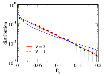
Figure 1: Distribution of numerically sampled decay probabilities $P_{b}$ (black circles) compared with the Porter-Thomas distributions for $\nu=1$ (dashed line) and $\nu=2$ (solid line). The dimension of the two GOE spaces are $N_{g}=100$ and their Hamiltonian parameters $v_{g},v_{k},v_{k^{\prime}},\Gamma_{g}$ are set to 0.1. The hopping matrix elements in the channel spaces are taken as $t_{i}=1$. The mean values and the root-mean-square (rms) deviations for the numerical sampling are calculated for 50 histogrammed runs, each of which is constructed for 500 samples.

To understand the deviation from the $\nu=1$ Porter-Thomas distribution, Fig. 2 shows the distribution of the probability $P_{b}$ for several values of $\Gamma_{a}$, setting $t_{2}=-(10\Gamma_{a})^{1/2}$ and keeping the other parameters the same as in Fig. 1. We wish to keep the expectation value $\langle P_{b}\rangle$ constant as $\Gamma_{a}$ is varied. This is achieved in the transition-state formula Eq. (38) of Ref. verA by changing $t_{2}$ as described. The two curves in each panel show the fits to the PT distribution with $\nu=1$ and $\nu=2$. When $\Gamma_{a}$ is much smaller than $v_{g}$ and $\Gamma_{b}$, as in Fig. 2(a), the distribution is consistent with the $\nu=1$ PT distribution. As $\Gamma_{a}$ increases, it gradually deviates from that, and eventually comes close to the $\nu=2$ PT distribution. We have checked that the distribution is insensitive to the decay widths in the second reservoir over a broad range of the parameter $\rho_{0b}\Gamma_{b}$.

We also carried out a least-squared fit of $\nu$ in the PT distribution to the histogrammed data with results shown in Fig. 3. It comes out close to $\nu=1$ for small control parameter $\rho_{0a}\Gamma_{a}$ and to $\nu=2$ for moderate and large $\rho_{0a}\Gamma_{a}$. We have also plotted on the Figure the function $\nu(y)=(1+8.28y^{2})/(1+3.81y^{2})$ with $y=\rho_{0a}\Gamma_{a}$ as a purely phenomenological description of fitted $\nu$ parameters.

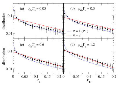
Figure 2: The distribution of the transmission probability for the second reservoir, $P_{b}$, for several values of $\Gamma_{a}$ and $t_{2}=-(10\Gamma_{a})^{1/2}$ as explained in the text. The dots with error bars were calculated with 50 histogrammed samplings as in Fig. 1. The dashed and the solid curves denote the $\nu=1$ and 2 PT distributions, respectively.

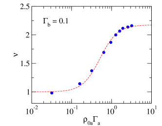
Figure 3: Fitted values to the number of degrees of freedom $\nu$ as a function of the control parameter $\Gamma_{a}\rho_{0a}$. The Hamiltonians are defined in the same way as in Fig. 2. The dashed line shows an empirical fit, $\nu(y)=(1+8.28y^{2})/(1+3.81y^{2})$ with $y=\rho_{0a}\Gamma_{a}$. Note that the $\nu$ exceeds 2 in the asymptotic region $\rho_{0a}\Gamma_{a}\gg 1$. This may be a finite size effect, but we have not examined this possibility.

Summary. Making use of random matrixx theory, we have applied a Hamiltonian to fluctuations in reactions of complex quantum systems. The model had been previously proposed to find the limits of validity of the transition-state theory of averaged reaction quantities. It is common wisdom that fluctuations in decay rates associated with a transition state in a time-reversal-invariant Hamiltonian follow the PT distribution for one degree of freedom. However, the effective Hamiltonian is complex when boundary conditions arising from other channels are taken into account. When those decay widths are comparable or larger than the average level spacing, the fluctuations approach the PT distribution for $\nu$ = 2. In the model, the key quantity responsible for fluctuations is the quantity $w_{23}$ which depends on Green’s function for the Hamiltonian of the first reservoir. For real Green’s functions the fluctuations are also real, corresponding to a single degree of freedom. However, if the states in the reservoir can decay directly into continuum channels, the Green’s function is complex and the fluctuations approach those of a complex quantity with independent variations in the real and imaginary parts. This behavior leads to reaction rates that follow the $\nu=2$ PT distribution. The model shows the crossover from one distribution to the other, with the control parameter identified as $\rho_{0a}\Gamma_{a}$.

A crossover from $\nu=1$ to $\nu=2$ has also been studied in random matrix models al98 ; al00 , interpolating between the GOE and the GUE ensembles. However, it is not clear from such studies how to relate the complex matrix elements to physical quantities when the underlying Hamiltonian is purely real.

The present model might be useful in the methodology for determining the effective number of channels in transition-state theory. In Ref. po90 the effective number of channels in a unimolecular reaction was estimated from a formula based on the $\nu=1$ PT distribution mi90 ,

$$\nu_{\rm eff}=2\langle\Gamma\rangle^{2}/(\langle\Gamma^{2}\rangle-\langle\Gamma\rangle^{2}).$$ (9)

The authors found that their theoretical calculations were a factor of two off. Depending on the direct decay widths of the initial molecule, the explanation might be the factor of two difference from the $\nu=1$ and $\nu=2$ PT distributions.

Previously, it has been shown in nuclear physics that a coupling to continuum state narrows the distribution, leading to $\nu$ which is smaller than one if the distribution is fitted with Eq. (1) CAIZ2011 . This was not realized in our model, as the value of $\nu$ was found to be between 1 and 2. In any case, it would be interesting if the deviation from the Porter-Thomas distribution discussed in that paper could be observed experimentally.

We thank Yoram Alhassid for linking the $\nu=2$ distribution to the fluctuations of $w_{23}$ in the complex plane. We also thank him, Yan Fyodorov, and Hans Weidenmüller for additional comments on the manuscript. This work was supported in part by JSPS KAKENHI Grant Numbers JP19K03861 and JP21H00120.

I Supplementary Material

I.1 Decay probability $P_{b}$

For completeness and to make the paper self-contained, we here provide a short derivation of the effective Hamiltonian (4). Call the vector of states that the Hamiltonian acts on

$$\boldsymbol{\Psi}=(\phi_{1},\phi_{2},\Psi_{a},\phi_{3},\phi_{4},\Psi_{b}).$$ (10)

The amplitudes $\phi_{1},\phi_{2}$ are the nearest ones in the entrance channel and $\phi_{3},\phi_{3}$ are in the bridge channel. $\Psi_{a}$ and $\Psi_{b}$ are sets of amplitudes for states in the GOE reservoirs. For a fixed amplitude $\phi_{1}$ the Hamiltonian equation

$$({\mathbf{H}}-E)\left(\begin{matrix}\phi_{1}\\ \phi_{2}\\ \Psi_{a}\\ \phi_{3}\\ \phi_{4}\\ \Psi_{b}\end{matrix}\right)=\left(\begin{matrix}0\\ 0\\ 0\\ 0\\ 0\\ 0\\ \end{matrix}\right)$$ (11)

can be solved for the remaining amplitudes by simple matrix operations. This is carried out in two steps. In the first step the amplitudes $\Psi_{a}$ are expressed in terms of $\phi_{2}$ and $\phi_{3}$. Similarly the amplitudes in $\Psi_{b}$ are expressed in terms of $\phi_{4}$. This reduces the Hamiltonian equation to the form

$$\left[\begin{matrix}w_{22}-E&w_{23}&0\cr w_{23}&w_{33}-E&t_{2}\cr 0&t_{2}&w_{44}-E\cr\end{matrix}\right]\left(\begin{matrix}\phi_{2}\cr\phi_{3}\cr\phi_{4}\cr\end{matrix}\right)=-\left(\begin{matrix}t_{1}\phi_{1}\cr 0\cr 0\cr\end{matrix}\right).$$ (12)

We next derive formulas for the decay probabilities following the lines presented in Ref. verA . For simplicity we restrict the energy to $E=0$, which is in the middle of the spectrum distributions of the GOE matrices in the Hamiltonian (2). Eq. (12) is easily solved for amplitudes $\phi_{2},\phi_{3}$ and $\phi_{4}$ in terms of $\phi_{1}$; the solution is

$$\phi_{2} =-(w_{33}w_{44}-t_{2}^{2})t_{1}\phi_{1}/D$$ (13)

$$\phi_{3} =w_{23}w_{44}t_{1}\phi_{1}/D$$ (14)

$$\phi_{4} =-w_{23}t_{2}t_{1}\phi_{1}/D$$ (15)

where

$$D=w_{22}w_{33}w_{44}-w_{22}t_{2}^{2}-w_{23}^{2}w_{44}.$$ (16)

The probability we seek can be expressed in terms of the probabilities fluxes $\Phi_{ij}$ from channel site $i$ to neighboring channel site $j$ as

$$P_{b}=\frac{\Phi_{34}}{\Phi_{12}}.$$ (17)

The individual fluxes are computed by the standard quantum relation

$$\Phi_{ij}=\langle i|H|j\rangle{\rm Im}(\phi_{i}\phi_{j}^{*}),$$ (18)

where $\langle i|H|j\rangle$ is the hopping matrix element between the two sites, that is, $\langle 1|H|2\rangle=t_{1}$ and $\langle 3|H|4\rangle=t_{2}$. The results are

$$\Phi_{12}=-2t_{1}^{2}\left[{{\rm Im}(w_{22})|s|^{2}-{\rm Im}(w_{23}^{2}w_{44}s^{*})}\right]\frac{1}{|D|^{2}}|\phi_{1}|^{2}$$ (19)

where $s=w_{33}w_{44}-t^{2}_{2}$ and

$$\Phi_{34}=-2t_{1}^{2}t_{2}^{2}|w_{23}|^{2}{\rm Im}(w_{44})\frac{1}{|D|^{2}}|\phi_{1}|^{2}.$$ (20)

The transmission factors are easily expressed in terms of the fluxes; for our purposes here we only need the ratio of the two fluxes given in Eq. (8).

I.2 Variances of self-energy quantities

Statistical properties of the GOE Green’s function have been derived in Refs. lo00 and (fe20, , App. C) for the limits given in Table I. We follow the same method here to determine the quantities needed in Eq. (8). The derivations are based on an eigenfunction representation of the self-energies,

$$w_{kk^{\prime}}=\sum_{j}^{N_{g}}\frac{\langle\mbox{\boldmath$v$}_{k}|\phi_{j}\rangle\langle\phi_{j}|\mbox{\boldmath$v$}_{k^{\prime}}\rangle}{E-E_{j}+i\Gamma_{g}/2}$$ (21)

where $E_{j}$ and $\phi_{j}$ are the eigenvalues and eigenfunctions of a GOE Hamiltonian of dimension $N_{g}$. The overlap $\langle\mbox{\boldmath$v$}_{k}|\phi_{j}\rangle$ is given by $\langle\mbox{\boldmath$v$}_{k}|\phi_{j}\rangle=v_{k}r_{j}$, where $v_{k}$ is a Hamiltonian parameter and $r_{j}$ is a Gaussian variable satisfying $\langle r_{j}r_{j^{\prime}}\rangle=\delta_{jj^{\prime}}$. The $r$ variables associated with different $\mbox{\boldmath$v$}_{k}$ vectors are distinguished as $r$ and $r^{\prime}$. They satisfy $\langle r_{j}r^{\prime}_{j^{\prime}}\rangle=0$.

We first consider an ensemble average of the diagonal self-energy, $w_{kk}$, at $E=0$. Since the eigenvector components are uncorrelated with each other or with the eigenenergies, the ensemble average can be expressed as

$$\langle w_{kk}\rangle=\langle(v_{k}r_{j})^{2}\rangle\left\langle\sum_{j}^{Ng}\frac{1}{-\tilde{E}_{j}}\right\rangle=v_{k}^{2}\left\langle\sum_{j}^{Ng}\frac{1}{-\tilde{E}_{j}}\right\rangle$$ (22)

where $\tilde{E}_{j}=E_{j}-i\Gamma_{g}/2$. By replacing the sum over $j$ by the energy integral with the level density $\rho(E)=\rho_{0}\sqrt{1-(E/E_{mg})^{2}}$, one obtains verA

$$\langle w_{kk}\rangle\approx v_{k}^{2}\rho_{0}{\cal I}_{1}(i\Gamma_{g}/2E_{mg})\approx-i\pi v_{k}^{2}\rho_{0}\,\,\,{\rm for}\,\,\,\Gamma_{g}\ll E_{mg},$$ (23)

where

$${\cal I}_{1}(z)=\int^{+1}_{-1}dx\frac{\sqrt{1-x^{2}}}{z-x}=\pi\left(z-\sqrt{z+1}\sqrt{z-1}\right).$$ (24)

taking the principal value of the square root.

To derive the formula for the variance of ${\rm Im}(w_{kk})$, we start with the equation for its second moment,

$$\langle[{\rm Im}(w_{kk})]^{2}\rangle$$

$$=\left<\sum_{ii^{\prime}}^{N_{g}}(\mbox{\boldmath$v$}_{k}\cdot\mbox{\boldmath$\phi$}_{i})^{2}(\mbox{\boldmath$v$}_{k}\cdot\mbox{\boldmath$\phi$}_{i^{\prime}})^{2}{\rm Im}\left(\frac{1}{\tilde{E}_{i}}\right){\rm Im}\left(\frac{1}{\tilde{E}_{i^{\prime}}}\right)\right>.$$

The numerator factors are $v_{k}^{4}r_{i}^{2}r_{j}^{2}$ in the new notation. The expectation value of the product of variables is

$$\langle r^{2}_{i}r^{2}_{j}\rangle =\langle r^{2}\rangle^{2}(1-\delta_{ij})+\langle r^{4}\rangle\delta_{ij}$$ (26)

$$=1+2\delta_{ij}.$$ (27)

Neglecting the fluctuation in the $E_{i}$, the expectation value becomes

$$\langle[{\rm Im}(w_{kk})]^{2}\rangle=v_{k}^{4}\left({\rm Im}\sum_{i}\frac{1}{\tilde{E}_{i}}\right)^{2}+2v_{k}^{4}\,\sum_{i}\left({\rm Im}\frac{1}{\tilde{E}_{i}}\right)^{2}.$$ (28)

The first term is just the square of $\langle{\rm Im}(w_{kk})\rangle$ and the second term is the variance.

As before, we replace the sums by an integral. In dimensionless form the required integral is ${\cal I}_{2}$ given by

$${\cal I}_{2}(y)=\int_{-1}^{+1}dx\frac{(1-x^{2})^{1/2}}{(x^{2}+y^{2})^{2}}=\frac{\pi}{2y^{3}\sqrt{1+y^{2}}}\approx\frac{\pi}{2y^{3}}.$$ (29)

Evaluating the integral at $y=\Gamma_{g}/2E_{m}$, one obtains for the variance

$$\langle[{\rm Im}(w_{kk})]^{2}\rangle-\langle{\rm Im}(w_{kk})\rangle^{2}=2\pi v_{k}^{4}\rho_{0}/\Gamma_{g}.$$ (30)

The variance for the real part of $w_{kk}$ can be evaluated in a similar way. Using the integral

$${\cal I}_{3}(y)=\int_{-1}^{+1}dx\frac{x^{2}(1-x^{2})^{1/2}}{(x^{2}+y^{2})^{2}}\approx\pi/2y,$$ (31)

one obtains

$$\langle[{\rm Re}(w_{kk})]^{2}\rangle-\langle{\rm Re}(w_{kk})\rangle^{2}=2\pi v_{k}^{4}\rho_{0}/\Gamma_{g},$$ (32)

which coincides with the variance of the imaginary part of $w_{kk}$.

Let us next consider the square of the absolute value of off-diagonal self-energies $w_{kk^{\prime}}$ at $E=0$ with $k\neq k^{\prime}$. To determine the expectation value of this quantity, we first express it as

$$\langle|w_{kk^{\prime}}|^{2}\rangle=v_{k}^{2}v_{k^{\prime}}^{2}\langle r_{i}r_{j}r_{i}^{\prime}r_{j}^{\prime}\rangle\left\langle\sum_{i,i^{\prime}}^{N_{g}}\frac{1}{\tilde{E}_{i}\tilde{E}_{i^{\prime}}^{*}}\right\rangle.$$ (33)

Using

$$\langle r_{i}r_{j}r_{i}^{\prime}r_{j}^{\prime}\rangle=\langle r_{i}r_{j}\rangle^{2}=\delta_{i,j},$$ (34)

one obtains

$$\langle|w_{kk^{\prime}}|^{2}\rangle=v_{k}^{2}v_{k^{\prime}}^{2}\frac{\rho_{0}}{E_{m}}{\cal I}_{4}(c)\approx 2\pi v_{k}^{2}v_{k^{\prime}}^{2}\frac{\rho_{0}}{\Gamma_{g}},$$ (35)

where $c=\Gamma_{g}/2E_{m}$, and ${\cal I}_{4}$ is given by

$${\cal I}_{4}(y)=\int_{-1}^{+1}dx\frac{(1-x^{2})^{1/2}}{(x^{2}+y^{2})}=\frac{\pi}{y}\left(\sqrt{1+y^{2}}-y\right)\approx\frac{\pi}{y}.$$ (36)

The separate variance of the real and imaginary parts of $w_{kk^{\prime}}$ can be evaluated in the same way using integrals ${\cal I}_{4}$ and ${\cal I}_{4}-y^{2}{\cal I}_{2}$ (see Eq. (41) below). Note that the integral required for the correlation $\langle({\rm Re}\,w_{kk^{\prime}})({\rm Im}\,w_{kk^{\prime}})\rangle$ vanishes identically.

The variance of $|w_{23}|^{2}$ is given by a product of four sums over eigenstates with 8 Gaussian variables in the numerator. The expectation value of the product is

$$\langle r_{i}r_{j}r_{k}r_{l}r^{\prime}_{i}r^{\prime}_{j}r^{\prime}_{k}r^{\prime}_{l}\rangle=\langle r_{i}r_{j}r_{k}r_{l}\rangle^{2}$$ (37)

$$=\langle r^{2}\rangle^{4}(\delta_{ij}\delta_{kl}+\delta_{ik}\delta_{jl}+\delta_{il}\delta_{jk})(1-\delta_{ijkl})$$

$$~{}~{}~{}~{}+\langle r^{4}\rangle^{2}\delta_{ijkl})$$ (38)

$$=(\delta_{ij}\delta_{kl}+\delta_{ik}\delta_{jl}+\delta_{il}\delta_{jk})+6\delta_{ijkl}.$$ (39)

Here $\delta_{ijkl}=\delta_{ij}\delta_{ik}\delta_{il}$. We next insert these restrictions into the sums over eigenstates. Two of the first three terms in Eq. (39) reduce the sums to $\langle{\rm Im}(w_{kk^{\prime}})\rangle^{2}$. The third term gives $\langle w_{kk^{\prime}}\rangle^{2}$ which we have seen can be neglected for physical parameter sets. For parameters sets such that the last term is also small, the variance is

$$\langle|w_{kk^{\prime}}|^{4}\rangle-\langle|w_{kk^{\prime}}|^{2}\rangle^{2}=\langle|w_{kk^{\prime}}|^{2}\rangle^{2}.$$ (40)

In a similar way, one finds

$$\langle{\rm Re}(w_{kk^{\prime}})^{2}\rangle-\langle{\rm Re}(w_{kk^{\prime}})\rangle^{2}$$

$$=\langle{\rm Im}(w_{kk^{\prime}})^{2}\rangle-\langle{\rm Im}(w_{kk^{\prime}})\rangle^{2}=\pi\rho_{0}\frac{v_{k}^{2}v_{k^{\prime}}^{2}}{\Gamma_{g}}$$ (41)

and

$$\langle[{\rm Re}(w_{kk^{\prime}}^{2})]^{2}\rangle-\langle{\rm Re}(w_{kk^{\prime}}^{2})\rangle^{2}$$

$$=\langle[{\rm Im}(w_{kk^{\prime}}^{2})]^{2}\rangle-\langle{\rm Im}(w_{kk^{\prime}}^{2})\rangle^{2}=4\left(\frac{\rho_{0}\pi}{\Gamma_{g}}\right)^{2}v_{k}^{4}v_{k^{\prime}}^{4}.$$

To check these estimates, we have compared them with a numerical sampling of the ensembles. The results for a few parameter sets are shown in Table 2; the agreement is quite satisfactory.

Notice that the integrals ${\cal I}_{1}$, ${\cal I}_{2}$, ${\cal I}_{3}$, and ${\cal I}_{4}$ correspond to the integrals $I_{1}$, $I_{4}$, $I_{5}$, and $I_{3}$ in Ref. verA , respectively.

$N_{g}$	Type	sampled	analytic
100	$w_{kk}$	$-(0.02\pm 0.48)-(1.02\pm 0.47)i$	$(0\pm 0.45)-(1\pm 0.45)i$
	$|w_{kk^{\prime}}|^{2}$	$0.23\pm 0.27$	$0.2\pm 0.2$
400	$w_{kk}$	$-(0.00025\pm 0.61)-(1.95\pm 0.55)i$	$(0\pm 0.63)-(2\pm 0.63)i$
	$|w_{kk^{\prime}}|^{2}$	$0.41\pm 0.41$	$0.4\pm 0.4$
900	$w_{kk}$	$-(0.083\pm 0.80)-(3.06\pm 0.77)i$	$(0\pm 0.77)-(3\pm 0.77)i$
	$|w_{kk^{\prime}}|^{2}$	$0.60\pm 0.66$	$0.6\pm 0.6$
1600	$w_{kk}$	$-(0.030\pm 0.91)-(4.06\pm 0.96)i$	$(0\pm 0.89)-(4\pm 0.89)i$
	$|w_{kk^{\prime}}|^{2}$	$0.83\pm 0.96$	$0.8\pm 0.8$

Table 2: Expectation values and statistical fluctuations of diagonal and off-diagonal self-energies associated with the coupling of channels to GOE ensembles. The GOE Hamiltonian parameters $v_{g},v_{k},v_{k^{\prime}},\Gamma_{g}$ are set to 0.1 and the hopping matrix elements $t_{i}$ are set to one. The entries labeled “analytic” were calculated with these parameters in the statistical formulas (30,32,40). The entries labeled “sampled” were obtained with 100 numerically calculated samples.

References

(1) E. Wigner, Ann. Math. 52, 548 (1955).
(2) F.J. Dyson, J. Math. Phys. 3, 140 (1962).
(3) T. Guhr, A. Müller-Groeling and H.A. Weidenmüller,
Phys. Rep. 299, 189 (1998).