C symbol=C, format=0 \newconstantfamilyM symbol=M, format=0 \newconstantfamilyB symbol=B, format=0 \newconstantfamilyb symbol=b, format=0 \newconstantfamilyS symbol=S, format=0
Multiphase modelling of glioma pseudopalisading under acidosis
Abstract
We propose a multiphase modeling approach to describe glioma pseudopalisade patterning under the influence of acidosis. The phases considered at the model onset are glioma, normal tissue, necrotic matter, and interstitial fluid in a void-free volume with acidity represented by proton concentration. We start from mass and momentum balance to characterize the respective volume fractions and deduce reaction-cross diffusion equations for the space-time evolution of glioma, normal tissue, and necrosis. These are supplemented with a reaction-diffusion equation for the acidity dynamics and lead to formation of patterns which are typical for high grade gliomas. Unlike previous works, our deduction also works in higher dimensions and involves less restrictions. We also investigate the existence of weak solutions to the obtained system of equations and perform numerical simulations to illustrate the solution behavior and the pattern occurrence.
Keywords: glioma pseudopalisade patterns, multiphase model, reaction-cross diffusion equations
MSC 2020: 92C15, 92C50, 35Q92, 35K55, 35K20.
1 Introduction
Glioblastoma is the most common type of primary brain tumors in adults, with a dismal prognosis. The histological features include characteristic patterns called pseudopalisades, which exhibit garland-like structures made of aggregates of glioma cells stacked in rows at the periphery of regions with low pH and high necrosis surrounding the occlusion site(s) of one or several capillaries [39]. Such patterns are used to grade the tumor and are essential for diagnosis [6, 23].
The few continuous mathematical models proposed for the description of pseudopalisade patterns [1, 27, 26, 30], involve systems of ODEs and PDEs which were set up in a heuristic manner or obtained from lower scale dynamics. They account for various aspects like phenotypic switch between proliferating and migrating glioma as a consequence of vasoocclusion and nutrient suppression associated therewith [1], interplay between normoxic/hypoxic glioma, necrotic matter, and oxygen supply [30], or tissue anisotropy and repellent pH-taxis, with [27] or without [26] vascularisation. The latter two works deduced effective equations for glioma dynamics from models set on the lower, microscopic and mesoscopic scales in the kinetic theory of active particles (KTAP) framework explained e.g., in [4]. Those deductions are in line with previous works concerning glioma invasion in anisotropic tissue [9, 10, 11, 14, 15, 16, 18, 31], which use parabolic scaling to obtain the equations for glioma evolution on the macroscale from descriptions of subcellular and mesoscopic dynamics. Here we propose yet another approach, relying on the interpretation of the relevant components (glioma, normal tissue, necrotic matter, and acidity) as phases in a mixture - with the exception of acidity, which is characterised by proton concentration in the volume occupied by the phases.
Multiphase models in the framework of mixture theory [2, 12] have been considered in connection with cancer growth and invasion, (arguably) starting with [7, 8] and followed by many others, involving different mathematical and biological aspects; see e.g. [17, 19, 32, 33, 34, 36, 37, 40] and references therein. Particularly [34] provides a comprehensive discussion of the classes of multiphase models, along with their strengths and drawbacks. Such models employ a population level description with conservation laws analogous to balance equations for single cells, with supplementary terms accounting for interphase effects. Thereby, the living cells and tissues are most often seen as viscous fluids, while the interstitial fluid is inviscid. Few of the existing models (e.g., [17, 34, 40]) are explicitly handling necrosis, which is, however, an important component of advanced tumors. Likewise, there are relatively few models accounting for chemoattracting or chemorepellent agents (e.g., [17, 37]), which are known to bias in a decisive way the expansion of the neoplasm and therewith associated dynamics of tumor cells and surrounding tissue. To our knowledge there are no multiphase models for glioma pseudopalisade development. In this context we propose such a model comprising necrotic matter as one of the phases in the mixture (although there are a few issues related to this approach, as mentioned, e.g. in [34]). As our main aim is to describe glioma behavior in an acidic environment fastly leading to extensive necrosis, we explicitly include these influences in our model. From the mass and momentum balance equations written for the phases composing the neoplasm and supplemented with appropriate constitutive relations, we then deduce, under some simplifying assumptions, a system of reaction-cross diffusion equations with repellent pH-taxis for the glioma cells and normal and necrotic tissues, also including a solenoidality constraint on the total flux. Our deduction has some similarities with that in [19], however is done in N dimensions instead of 1D, it accounts explicitly for the evolution of necrotic matter and the effects of acidity, and does not require the drag coefficients between the phases to be equal. The obtained equations are able to reproduce qualitatively the typical pseudopalisade patterns with all their aspects related to the glioma aggregates, acidity, necrotic inner region, normal tissue dynamics.
The rest of this paper is organized as follows: Section 2 contains some notations and conventions. Section 3.1 contains the model setup with the considered phases (glioma cells, normal tissue, necrotic matter, and interstitial fluid) and the corresponding mass and momentum balance equations, along with their associated constitutive relations. That description is used to deduce the announced reaction-cross diffusion equations. Thereby, we investigate a model with an immovable component and observe that enforcing one of the phases to be fixed prevents the simultaneous validity of all basic conservation laws needed in the setting. Then we neglect the interstitial fluid, thus reducing the number of phases, and obtain the PDEs with reaction, nonlinear diffusion and taxis terms, while still ensuring all balance equations. The total flux needs to be given, satisfying a solenoidality constraint. Section 4 is dedicated to the existence of weak solutions to the obtained cross diffusion system coupled with the reaction-diffusion equation for acidity dynamics in the volume of interest. Finally, in Section 5 we provide numerical simulations for that system, studying several parameter scenarios in order to put in evidence the effect of acidity and of different drag coefficients on the obtained patterns exhibiting pseudopalisade formation.
2 Preliminaries
We will use the following notation throughout this paper:
Notation 2.1.
-
1.
By vector we always mean a column vector.
-
2.
We denote by the vector of length and all components equal to one. As usual, stands for the identity matrix of size .
-
3.
For two vectors and of the same length we denote by the vector with elements . Similarly, for a vector with nonzero elements we write meaning the vector with coordinates .
-
4.
For a vector we denote by the diagonal matrix with .
-
5.
As usual, denotes the scalar product.
-
6.
As usual, refers to the gradient with respect to the spatial variable .
Notation 2.2.
Throughout the paper we often skip the arguments of coefficient functions.
3 Modelling
3.1 Model setup
Model variables
Motivated by the multiphase approach developed in [19] we view the tumour and its environment as a saturated mixture of several components. We assume these components to be: tumour cells, normal tissue (mainly the extracellular matrix, but also normal cells), necrotic tissue (was not included in [19]), and interstitial fluid. The latter, in turn, has several constituents, among which are protons. Depending on their concentration, the environment can be more or less acidic. pH levels drop due to enhanced glycolytic activity of neoplastic cells. We assume that neither cells nor living tissue are produced due to an already very acidic, and hence very unfavourable, environment. Thus we assume that the total volume of the mixture is preserved, the phases only transferring from one into another. The main variables in our models, all depending on time and position in space , a domain, are:
-
•
vector of volume fractions of
-
–
tumour cells, ,
-
–
normal tissue, ,
-
–
necrotic tissue, ,
-
–
interstitial fluid, .
-
–
-
•
acidity (concentration of protons), .
Unlike [19] we do not require the space dimension, , to be one. The main goal of this Section is to derive equations for the volume fractions based primarily on the conservation laws for mass and momentum as well as additional assumptions on some of the phases. To write down the physical laws, we introduce additional variables that are subsequently eliminated. These are:
-
•
fluxes of the components, , ,
-
•
common pressure, .
Model parameters
The equations we develop below involve the following set of parameters:
-
•
matrix of drag coefficients associated with each pair of components, ;
-
•
additional, isotropic pressures by the components, , ;
-
•
reaction terms, , ;
-
•
diffusion coefficient of the protons, .
Assumptions on .
We assume throughout that
Assumptions on ’s.
In order to ensure that the sum of all volume fractions in the mixture is always one, we require
| (3.1) |
Since ’s and should be nonnegative, we require further that
Possible choices for the reaction terms are:
Example 3.1.
, , , . This accounts for the fact that the amount of both tissue and viable cancer cells (the latter being in interaction with the necrotic matter embedded in the acidic environment) decreases when the proton concentration exceeds a certain maximum threshold, leading to acidosis and hypoxia. The tissue infers degradation due to causes other than direct influence of acidity or tumor cells, and, on the other hand, it experiences a certain amount of self-regeneration, which is limited by the already available tissue and low pH. Thereby, are constant rates; they could, however, also include further dependencies. For the reaction term in the acidity equation we choose e.g., , with () constants. This choice ensures proton uptake by the interstitial fluid (with saturation), production by glioma cells, and decay with rate .
Assumptions on ’s.
We assume that the non-living components (necrotic matter and extracellular fluid) acquire a tendency to reach equilibrium, so that only living matter exerts additional pressure, thus
| (3.2) |
The mechanical properties of living matter (tumour cells and normal tissue) are different; among others, they are able to generate both intra- and interphase forces in response to changes in the local environment. The influences include variations in the volume fraction of the cell phase and the presence of chemical cues, of which we account for the local acidity (via proton concentration). The corresponding forces manifest themselves as an additional intraphase pressure. It is assumed that the pressure in the tumour and normal tissue phases increases with their respective densities; moreover, glioma cells exert supplementary (isotropic) pressure on the normal tissue. Taking these effects into account, we choose for the additional pressure terms
| (3.3) | |||
| (3.4) |
where are constants. In 3.3 we combine the influence of local cell mass and acidity, both adding to cancer cell pressure which, in turn, enhances glioma motility. Cell stress increases with growing cell mass, pushing the cells away from overcrowded regions. Stress due to acidity saturates for large acidity levels. Indeed, in highly acidic regions cell ion channels and pH-sensing receptors are mostly occupied, thus making cells insensitive to the presence of protons in their environment. As in [11, 24, 26, 27], we call this a repellent pH-tactic behaviour. Similarly, the choice in (3.4) means that there is some intraspecific tissue stress (compression) further accentuated by the interaction between glioma cells and their fibrous environment. The forms proposed in (3.3), (3.4) are reminiscent of those chosen in [19].
Main equations
To derive our models we will rely on a set of equations describing physical laws. They are as follows.
-
•
Since the the components of are volume fractions, we have
(3.5) This is the so-called ’no void’ condition.
-
•
Mass conservation for th component is given by
(3.6) It would be reasonable to assume that this equation should hold for all phases. However, this may come into conflict with additional assumptions, see subsequent Subsection 3.2.
-
•
Conservation of momentum for th component is given by
(3.7) where
(3.8) is the stress tensor involving the common pressure and the additional pressure . It is assumed that the response of the tumour to stress is elastic and isotropic, which implies that the deformation induced by the applied force on each of the considered cellular and tissue components is limited. An unlimited deformation would correspond to a viscoelastic material [20], which is not considered here. The forms of the stress tensors depend on the material properties of each phase and their response to mechanical and chemical cues in the environment. As in [19, 28] the interstitial fluid is considered to be inert and isotropic and viscous effects within each phase are neglected.
The right hand side in (3.7) represents the force acting on the th phase and, neglecting any inertial effects and exterior body forces, it takes the following form:
(3.9) The first term on the right hand side in (3.9) accounts as usual (see, e.g. [7, 19, 28]) for the pressure distribution at the interface between phases. The remaining term represents viscous drag between the phases, with drag coefficients .
-
•
The proton concentration satisfies the reaction-diffusion equation
(3.11)
In the remainder of this section we derive two models based on these laws. To begin with, we simplify equation 3.10. Given that and are scalar functions, we have for all
| (3.12) |
Since is symmetric, adding together the left-hand sides of 3.12 for all , we find that
| (3.13) |
Combining 3.12 with 3.5 and 3.13, we obtain
so that
| (3.14) |
Plugging 3.14 into 3.12 we arrive at a system which no longer involves :
| (3.15) |
and it holds that
| (3.16) |
Next, we introduce a matrix function
| (3.17) |
The symmetry of once again implies that
| (3.18) |
System 3.15 can now be written in the form
| (3.19) |
where we denote by the vector made up of the th coordinates of each . Due to 3.16 and 3.18 for each (at least) one equation is redundant. We exploit this in more detail in the next Subsections.
3.2 A model with an immovable component
Recall that and correspond to normal and necrotic tissues, respectively. A standard modelling assumption is that any tissue is completely immovable. This means that its flux is a zero function, turning the mass conservation law 3.6 into an ODE. However, as we show in this Section, already presupposing, e.g.
| (3.20) |
is problematic.
Singling out the th phase, we use the following convenient notation.
Notation 3.2.
For a vector with components corresponding to the four phases we denote by the vector which is obtained by removing the component which corresponds to th phase. Similarly, for a matrix we denote by the submatrix which results from removing the row and column of corresponding to that phase.
Recall that fluxes , , satisfy system 3.19 which is underdetermined. We notice that the submatrix is diagonal-dominant due to 3.18 and the nonnegativity of ’s and ’s. Using the Gershgorin circle theorem, we infer that the real parts of the eigenvalues of do not exceed , where
| (3.21) |
Therefore, for the submatrix of is invertible. Consequently, system 3.19-3.20 is uniquely solvable.
To simplify the calculations, let us now assume that the following technical assumption holds:
| (3.22) |
In other words, the symmetric matrix has rank one. One readily verifies the following formulas:
Lemma 3.3.
Using 3.25 we can resolve system 3.19-3.20 with respect to the components of the fluxes. For and we obtain
| (3.26) |
We used 3.5 and 3.2 in the third and fourth equalities, respectively. Plugging 3.26 into 3.6 and using 3.2, we obtain
| (3.27a) | |||
| (3.27b) | |||
For variable we have due to 3.6 and 3.20 that it satisfies an ODE:
| (3.28) |
However, the structure of the fluxes in 3.27 would ensure 3.5 only if
This condition fails to hold in general, unless for and such that
| (3.29) |
It is not fulfilled by the coefficients we have in mind, see Subsection 3.1.
Let us assume that 3.27 holds only for . Assume further that
| (3.30) |
i.e. that the liquid phase is negligible. In this case we obtain a haptotaxis model:
| (3.31a) | |||
| (3.31b) | |||
| (3.31c) | |||
| (3.31d) | |||
Unless is zero for , this model cannot ensure .
Altogether we see that trying to explicitly enforce an immovable phase leads to a situation where not all basic conservation laws can hold at the same time.
3.3 A model with total flux control
Let us now assume that the number of components in the mixture is three since
thus, unlike previous multiphase models in a related context (see e.g. [19, 37]), but compare also [36], we neglect the interstitial fluid and only take into account the more ’solid’ components, namely cancer cells, necrotic matter, and normal tissue, all of which are assumed to be more or less heterogeneously interspersed within the volume of interest. In this Subsection we assume all physical laws from Subsection 3.1 to hold in full, so that, in particular, the mass conservation law 3.6 holds for each . Due to 3.1 and 3.5 we can replace 3.6 for by
| (3.32) |
where
As we have seen previously, system 3.19 is underdetermined. However, if is given, then the system is equivalent to the following matrix equation:
| (3.33) |
where
| (3.34) |
and
One can readily verify that
where
| (3.35) |
Using 3.5, we can rewrite (3.3) as
| (3.36) |
where
| (3.37) |
| (3.38) |
Resolving 3.33 with respect to ’s and using 3.36, we get
| (3.39) |
Combining 3.37, 3.38, and 3.39, we obtain
| (3.40) |
and
| (3.41) |
Recalling that due to 3.2, we conclude from 3.40-3.41 that
| (3.42) |
and, similarly,
| (3.43) |
Set
| (3.44) | |||
| (3.45) | |||
| (3.46) | |||
| (3.47) |
Then 3.42 and 3.43 take the form
| (3.48) | |||
| (3.49) |
Finally, combining 3.5, 3.6, 3.48, 3.49, 3.32, 3.2, 3.3, and 3.4 we arrive at the system
| (3.50a) | |||
| (3.50b) | |||
| (3.50c) | |||
| (3.50d) | |||
Our construction guarantees that satisfies an equation similar to 3.50a and 3.50b:
| (3.51) |
where
and
This a priori ensures that is satisfied if the solution components are smooth.
Remark 3.4.
Remark 3.5.
Our allowing the tissues to be displaced (thus giving up the hypothesis of their immovability) led to nonlinear diffusion and drift in (3.50b) (or, for that matter, in (3.51)). This might seem unusual, as most reaction-difusion-transport systems describing cell motility in tissues assume the latter fixed and use ODEs for their evolution. We emphasize that the obtained terms do not state a self-driven motion of these components, but rather the effect of population- and biochemical pressure exerted thereon.
Remark 3.6.
To close model 3.50, one needs to choose some divergence-free . In dimension one and for no-flux boundary conditions is the only option. In higher dimensions can be a curl field (in ) or, more generally in dimensions (cf. [3]), an exterior product of gradients: . In the physically relevant case this means that , thus there exist some scalar quantities (e.g., densities/volume fractions/concentrations) such that the total flux is orthogonal to each of their gradients, or, put in another way, is tangential to a curve which lies in the intersection of the surfaces described by and . This would mean that the total flux is following a direction which is equally biased by those two species. The solenoidality of is a reasonable assumption in view of our previous requirement that there were no sources or sinks of material, either.
Diffusion matrix
Without loss of generality we assume that
| (3.52) |
One readily verifies that
| (3.53) |
where
| (3.54) | |||
| (3.55) | |||
| (3.56) |
Due to assumptions 3.52 we have for that
| (3.57) | |||
| (3.58) |
In particular, for small matrix 3.53 can be regarded as a perturbation of matrix
corresponding to
i.e. to
This case was addressed in [22]. Further, we compute
| (3.59) |
Overall, the diffusion matrix of equations 3.50a and 3.50b takes the form
| (3.60) |
The complete diffusion matrix of 3.50a, 3.50b, and 3.11 includes the third line
| (3.61) |
4 Existence of weak solutions to 3.50a-3.50c, 3.11
In this Section we use the method that was presented in [21] in order to establish an existence result for our cross diffusion system 3.50a-3.50c, 3.11. The key to applying the method is finding a suitable so-called entropy density. Motivated by the study in [22], where the case of equal ’s and no acidity was treated, we consider the following entropy density:
| (4.1a) | |||
| (4.1b) | |||
| (4.1c) | |||
| (4.1d) | |||
Here is the well-known logarithmic entropy and is a sufficiently large constant yet to be fixed. For the subsequent computations we need the matrix of second-order partial derivatives of :
| (4.2) |
In order to be able to apply the method from [21], we need to ensure positive (semi-)definiteness of matrix in where is the diffusion matrix of 3.50a, 3.50b, and 3.11. In this Subsection we verify this property for the parameter values satisfying the following conditions:
| (4.3) |
and
| (4.4) |
where and are constants defined in 3.54.
Remark 4.1.
Lemma 4.2 (Uniform ellipticity).
Proof.
To begin with, we compute
| (4.6) |
where
so that
| (4.7) |
Combining 4.2, 4.6, 3.60, and 3.61, we obtain (arguments of functions are omitted)
| (4.8) |
We introduce the symmetric matrix
where
| (4.9) |
Next, we study in . We compute
Observe that is quadratic with respect to , and the coefficient of is negative. Consequently, cannot attain its minimum inside . It remains to ensure that is positive on the sets and . This the case if
| (4.10) |
and
| (4.11) |
By Sylvester’s criterion, is positive definite if and only if is positive definite and . Due to 3.57-3.58, 4.7, and Lipschitz all functions involved in 4.9 are bounded and functions have positive lower bounds in . In particular, , so that is positive definite if and only if . Further, we have
where is a bounded function (recall that is Lipschitz). Thus, for sufficiently large , holds provided that . Altogether, we conclude that conditions 4.10 and 4.11 imply that matrix is positive for all triples in . Assuming these conditions to be satisfied, let denote an eigenvalue of . Then
In , functions and are bounded from above and from below, respectively, by some positive constants. Hence, we have positive lower and upper bounds for the eigenvalues of . ∎
Now we are ready to state our existence result.
Theorem 4.3.
Let and be some constants which satisfy 4.3, 4.4, and 3.54. Let coefficients and be as defined in 3.3 and 3.4 and let Lipschitz functions , with domain as in 4.1a, be such that
| (4.12a) | ||||
| (4.12b) | ||||
| (4.12c) | ||||
Then for every given and such that for a.a. there exists a weak solution to system 3.50a-3.50c, 3.11 under no-flux boundary conditions. This means that:
| (4.13) |
| (4.14a) | ||||
| (4.14b) | ||||
| (4.14c) | ||||
a.e. in for all , and the initial conditions for each variable are satisfied in -sense.
Remark 4.4.
Proof of Theorem 4.3 (sketch). We rely on the theory of weak solvability for cross diffusion systems which was developed in [21]. We recall that the main tool of the method in [21] is a suitable entropy density. Here we use function previously defined in 4.1. This function is the sum of the standard logarithmic entropy for variables and and the quadratic . Combining the corresponding properties of the logarithmic entropy and our previous calculations in this Section, we obtain:
-
H1:
and is convex and bounded below by
The derivative
(4.15) is invertible, the inverse being
-
H2’:
For sufficiently large , left multiplying the diffusion matrix by yields a uniformly positive definite matrix (see Lemma 4.2).
- H2”:
-
H3:
and , , are continuous mappings and there exists a constant such that
(4.16)
Estimate 4.16 is a standard consequence of the assumptions 4.12. Indeed, since is negative and bounded below in , the part originating from the logarithmic entropy satisfies
| (4.17) |
for some constant . Further, since is Lipschitz, we also have
| (4.18) |
for some constant . Adding 4.17 and 4.18 together, we obtain
since obviously . The main result of [21], Theorem 2 on existence of bounded weak solutions, cannot be directly applied in our case for two reasons: firstly, apart from diffusion and reaction, equations for and also involve transport in the direction of a given vector-valued function ; secondly, the domain is not bounded. Were it not for these differences, the above properties H1-H3 would correspond to the hypotheses H1-H3 in [21]. Still, the proof of existence of weak solutions can be carried out very similar to the proofs presented in [21]. The latter go through the following steps: approximation of the time derivative using the implicit Euler scheme, regularisation of the diffusion operator by adding a higher order differential operator such as for and small , solving the linearised approximation problem using the Lax-Milgram lemma, solving the nonlinear approximation problem using the Leray-Schauder theorem, establishing uniform estimates, and, finally, using the compactness method in order to pass to the limit and solve the original problem. Our case can be handled in the very same way. Indeed, on the one hand the linear transport along is subordinate to diffusion, so that it, e.g. does not hinder the derivation of estimates. On the other hand even though is not bounded, we actually know that for bounded the -component of a solution is a priori bounded on all finite time cylinders. This is a consequence of the standard theory of semilinear parabolic PDEs. General can be regularised and a corresponding solution obtained by means of yet one more limit procedure. We omit further details and refer the interested reader to [21] where the complete proofs for very similar cases can be found. ∎
5 Numerical study
We perform numerical simulations of the system (3.50) supplemented with the PDE (3.11) for the evolution of proton concentration , endowed with no-flux boundary conditions. For simplicity we choose . We also perform a nondimensionalisation of the model and use it in our simulations (for its concrete form and for the employed parameters refer to the Appendix). The initial conditions are as follows:
| (5.1a) | ||||
| (5.1b) | ||||
| (5.1c) | ||||
| (5.1d) | ||||
These are illustrated in Figure 1. The problem is set in a square (in ), corresponding to the size of large pseudopalisades [5]. For the discretisation we use a method of lines approach. Thereby, the diffusion terms in all involved PDEs are computed by using a standard central difference scheme, while a first order upwind scheme is employed for the advection terms occurring in the equations for glioma and normal tissue. For the acidity equation we discretise time upon using an implicit-explicit (IMEX) method, with forward and backward Euler schemes for the diffusion and reaction terms, respectively. The glioma and normal tissue PDEs are discretised in time by an explicit Euler method.
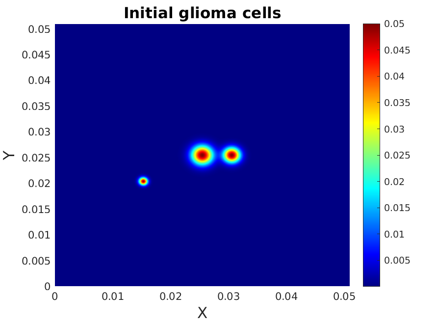
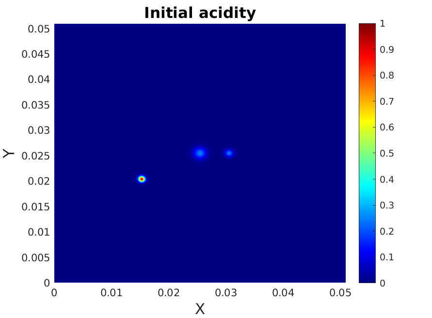
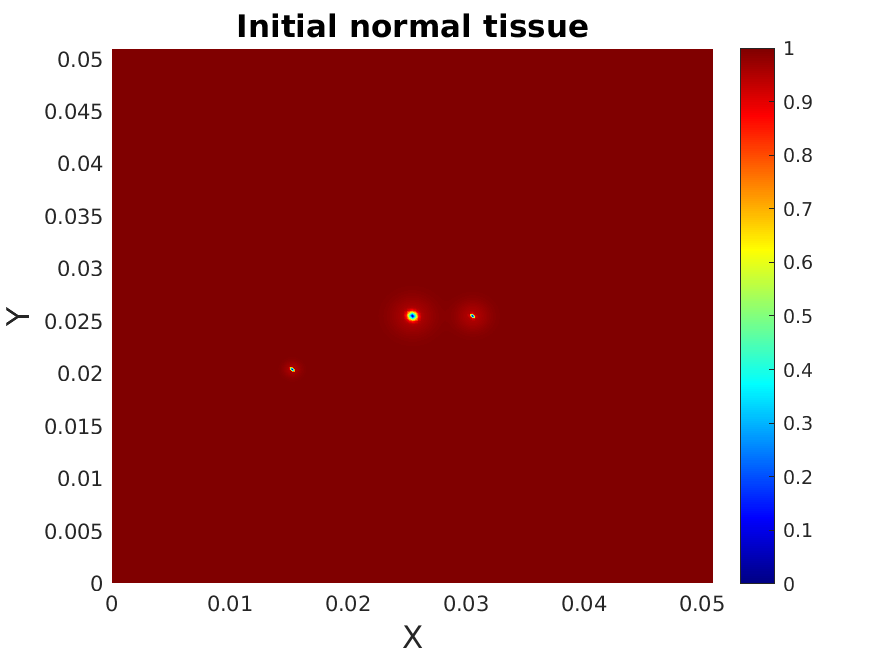
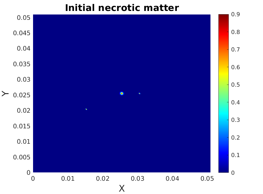
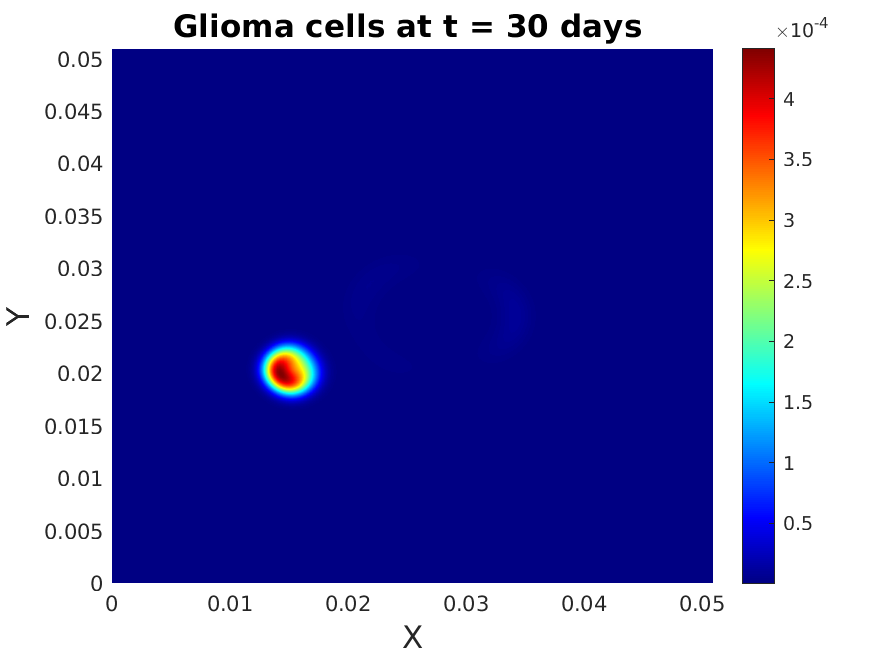
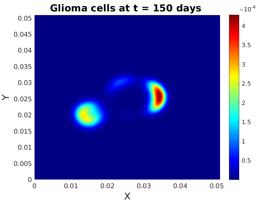
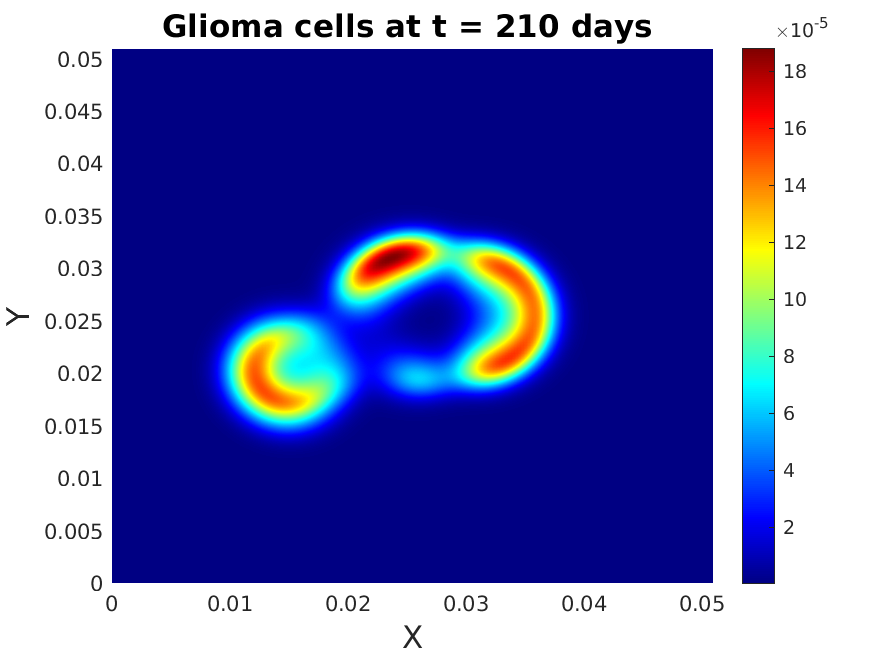
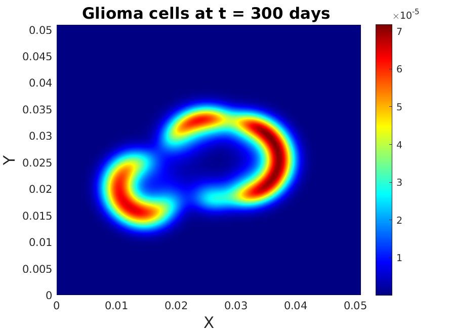
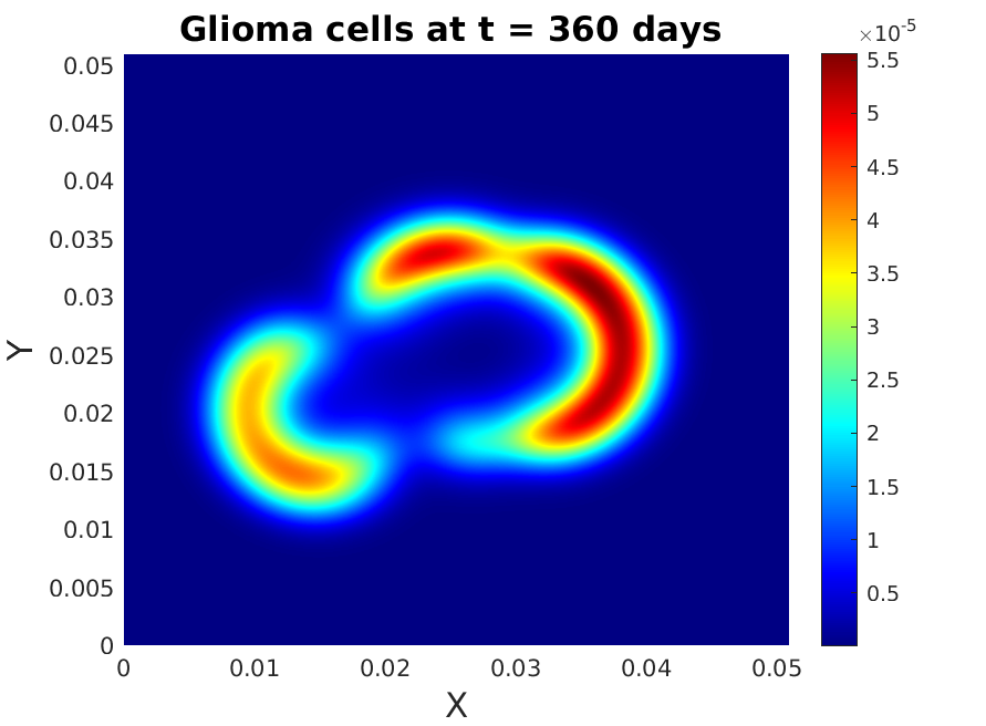
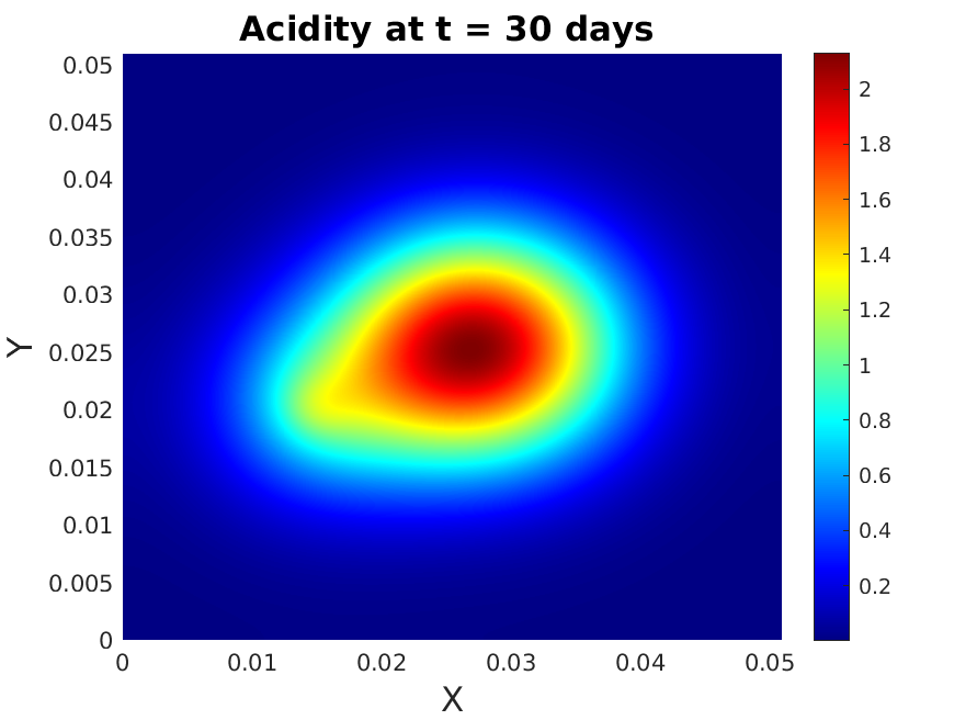
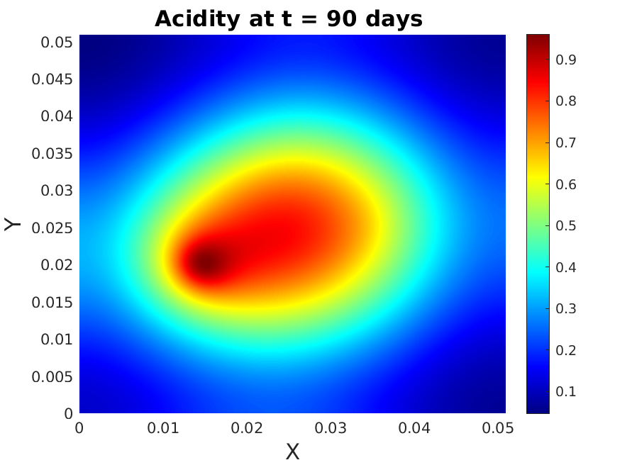
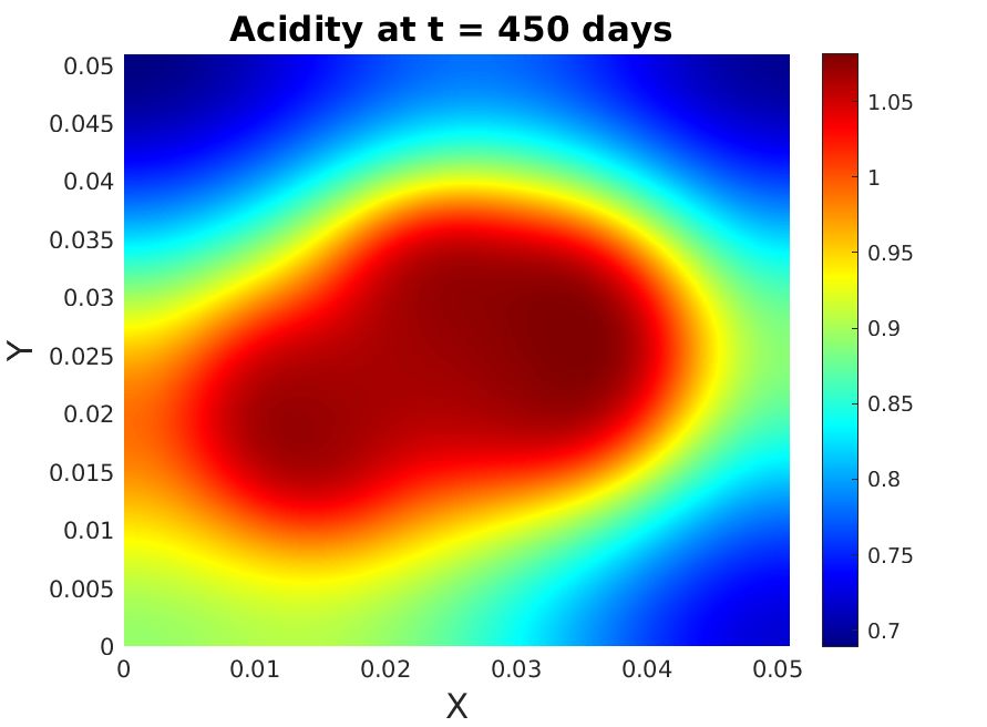
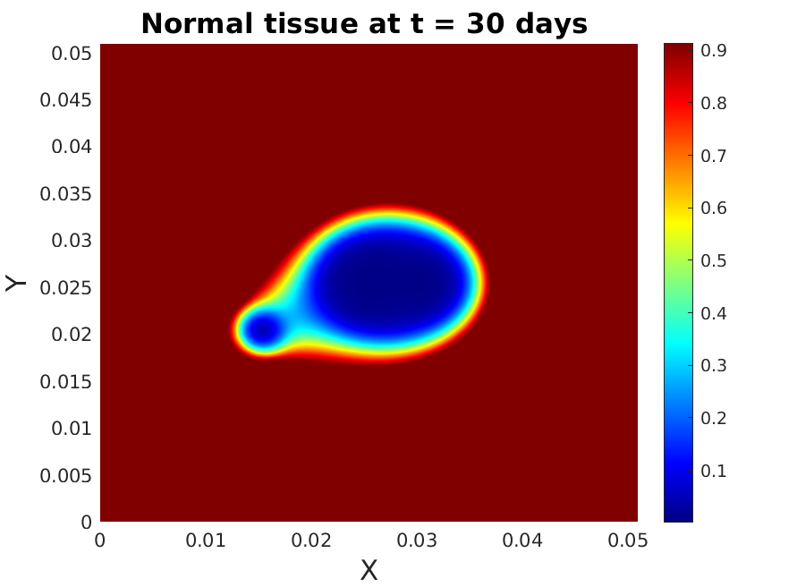
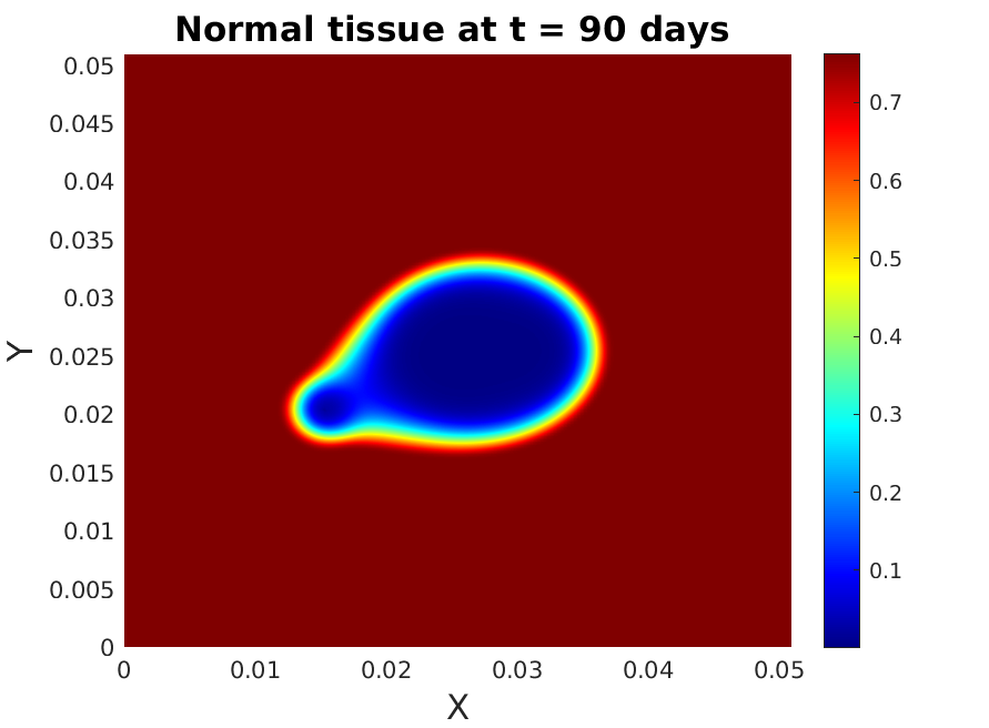
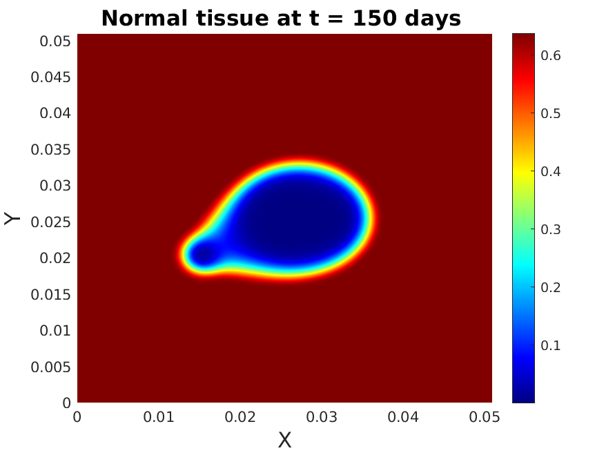
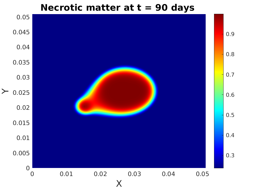
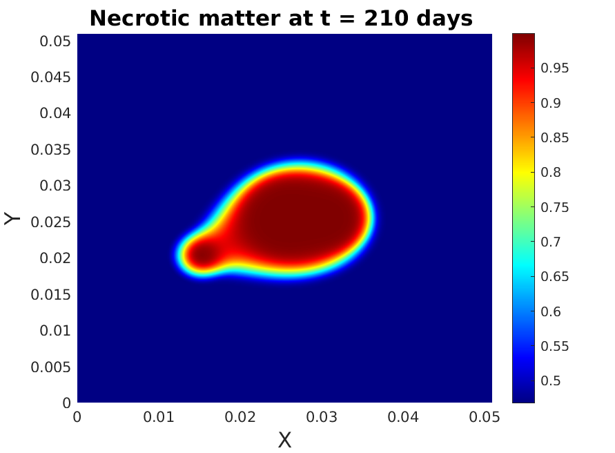
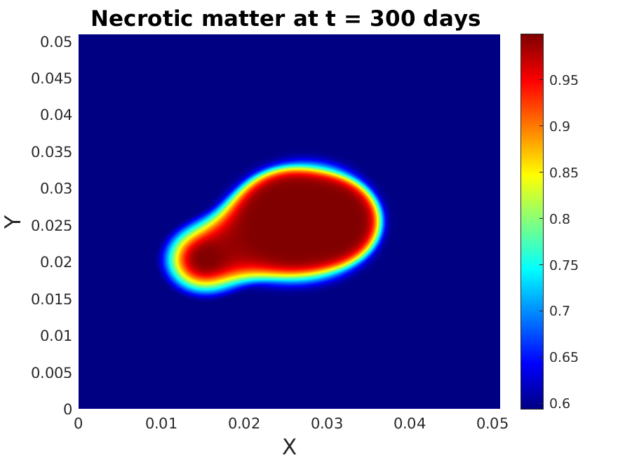
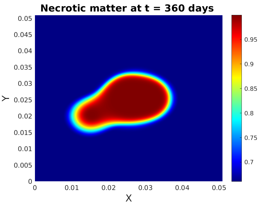
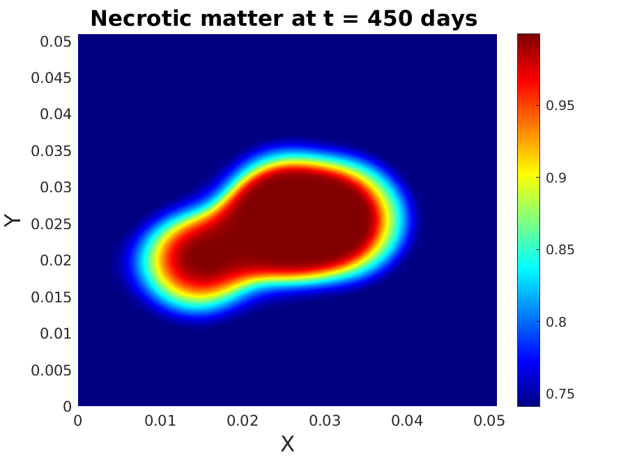
Figure 2 shows the computed volume fractions of glioma (first column), normal tissue (3rd column), necrotic matter (last column), and acidity concentration (second column) at several times, in a total time span which is relevant for pseudopalisade formation. The typical garland-like structure of glioma pseudopalisades is clearly visible. The tumor cells encircle a highly acidic and necrotic region, while outwards, beyond the glioma ring, the normal tissue remains non-depleted and the acidity decreases.
30 days
90 days

150 days
210 days
300 days
360days
450 days
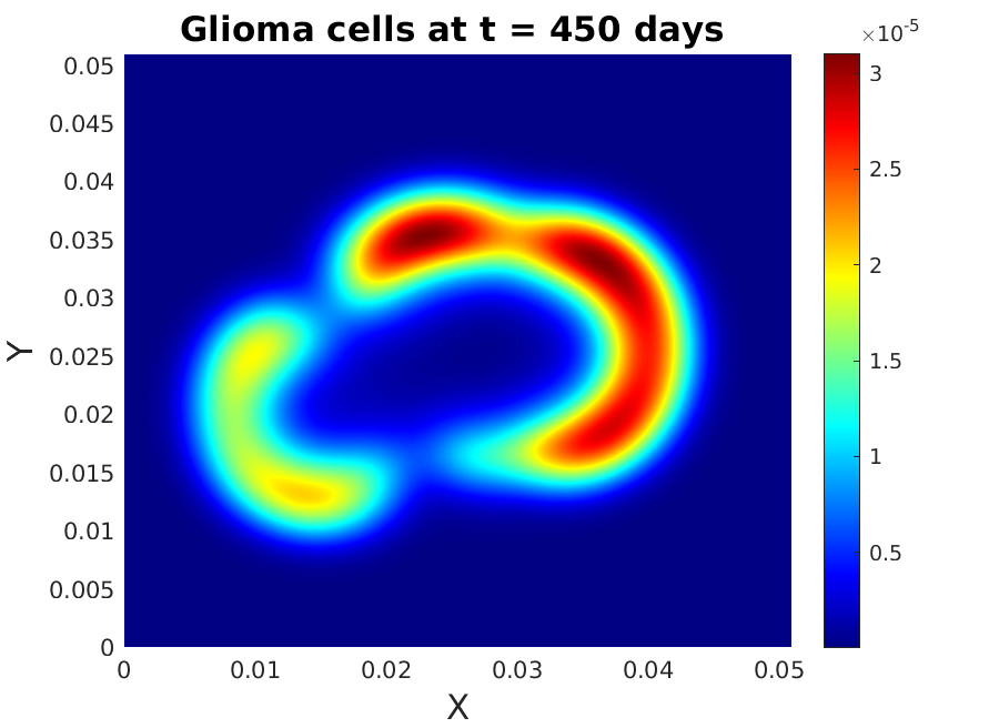
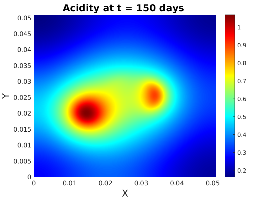
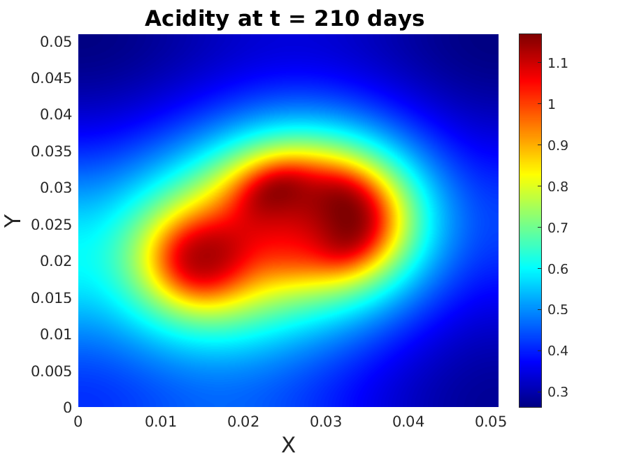
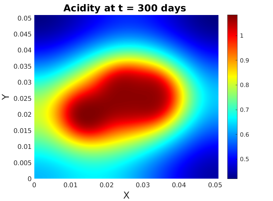
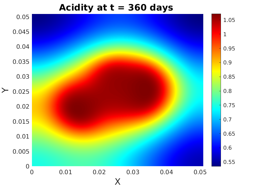
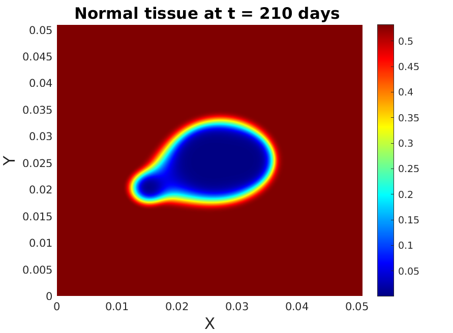

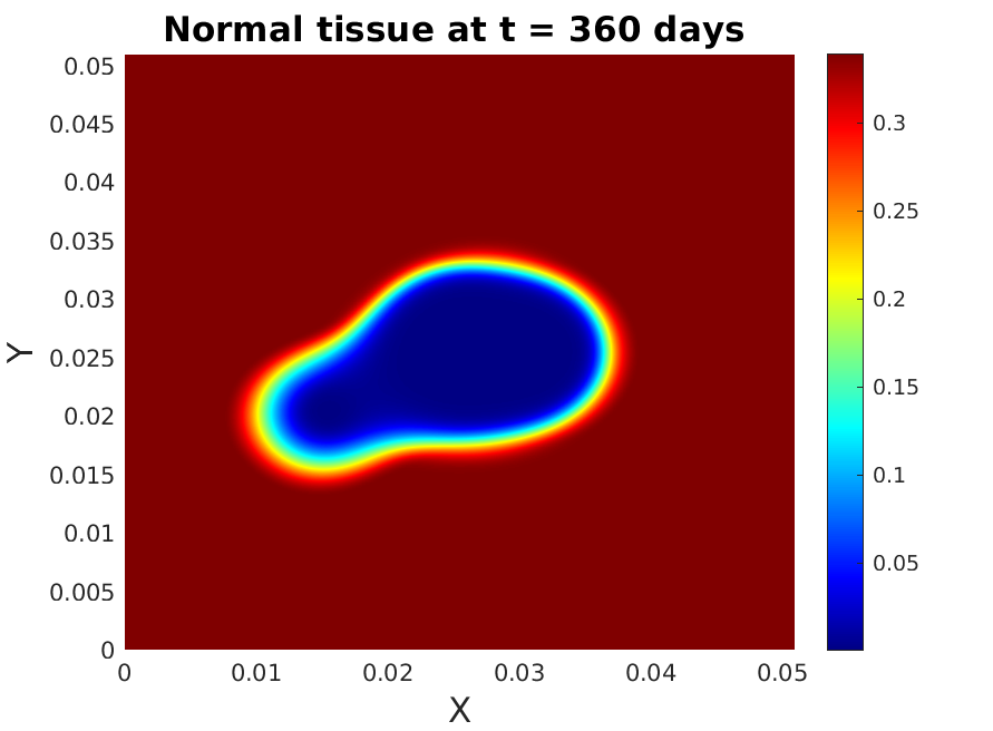
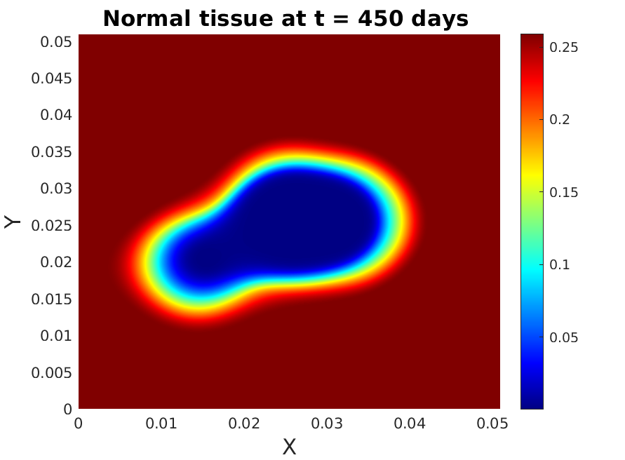
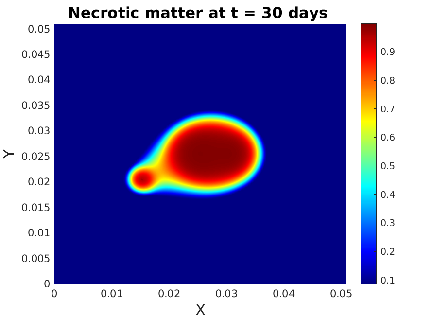

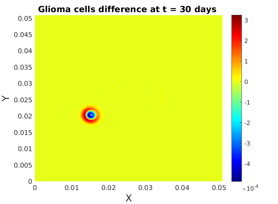
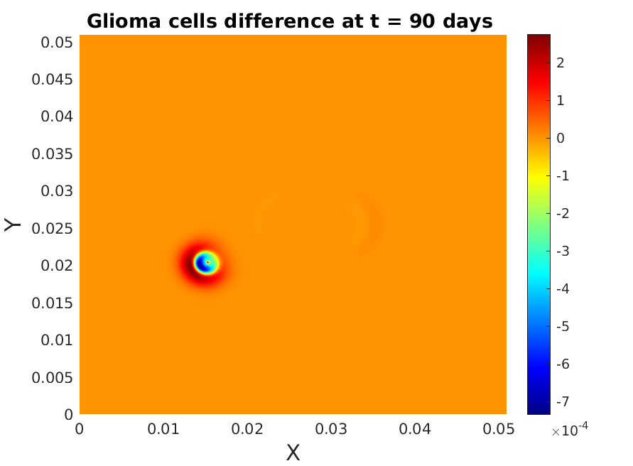
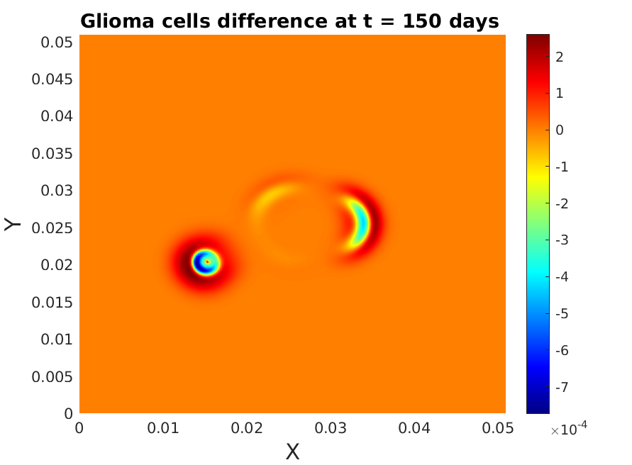
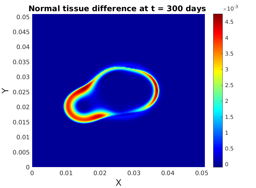
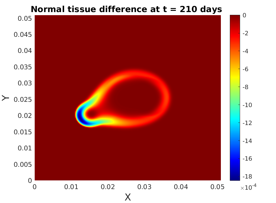
To investigate the effect of acidity we compare the previous results with those obtained for , i.e. in the absence of additional pressure on glioma cells due to acidosis, recall (3.3). The corresponding plots are shown in Figure 3. The effect of repellent pH-taxis can be seen in the difference between the solution components in two situations (with , with pH-taxis and acid-influenced motility, respectively with ). The pseudopalisades develop faster and get thicker and more extensive in the former case, accompanied by enhanced acidity in the proximity of higher cancer cell densities and enhanced normal tissue depletion inside the ring-shaped structures and around the glioma aggregates, which also triggers a higher volume fraction for the necrotic matter. These observations are in line with those obtained in [26] by another modeling approach: the repellent pH-taxis is not the driving factor of pseudopalisade formation, but it leads to wider such structures.
30 days
90 days
150 days
210 days
300 days
360 days
450 days
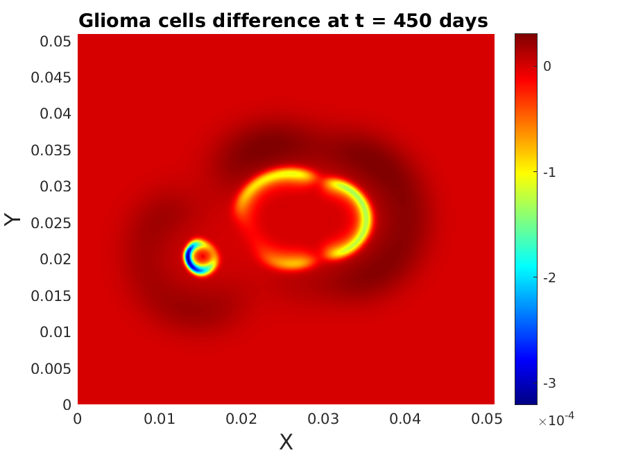
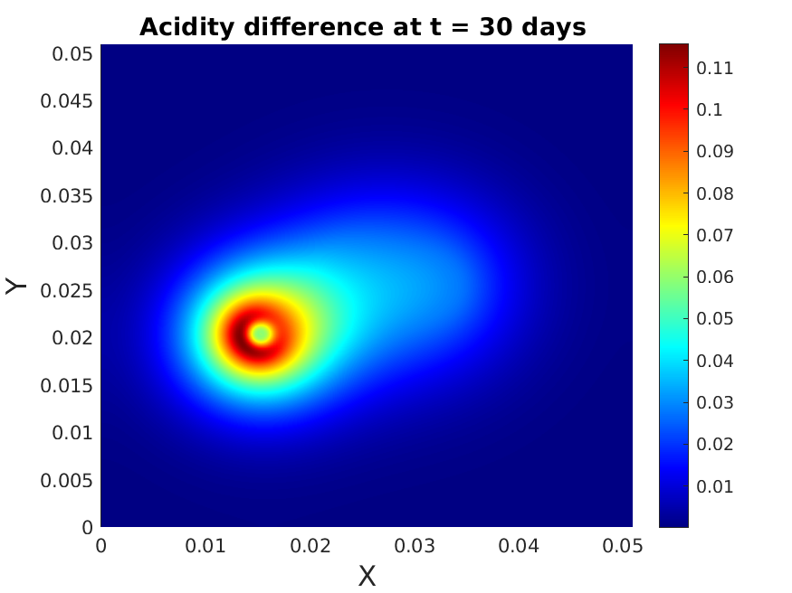
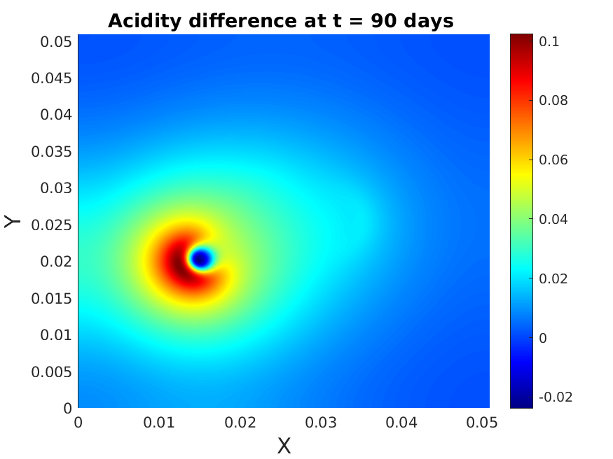
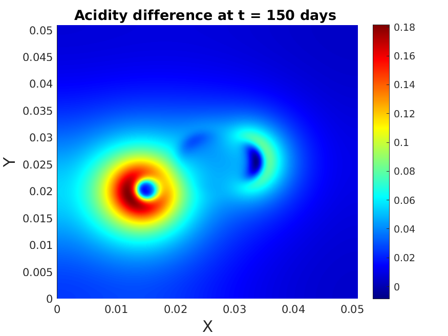
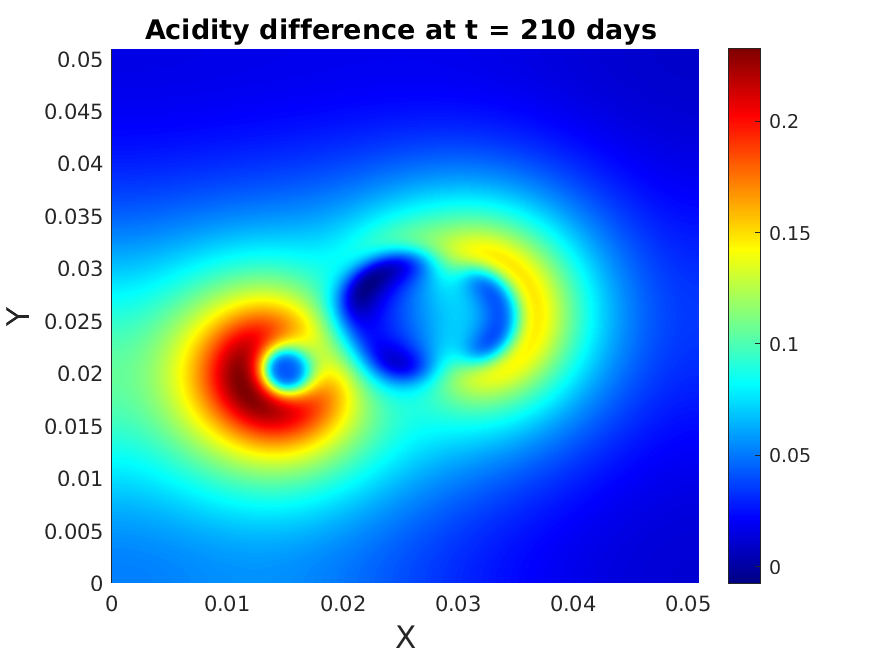
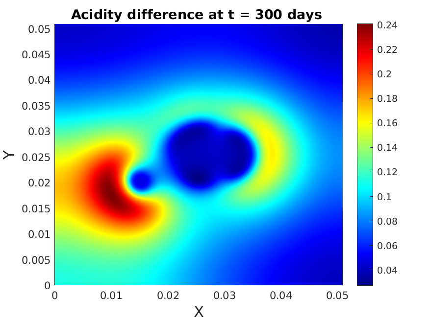
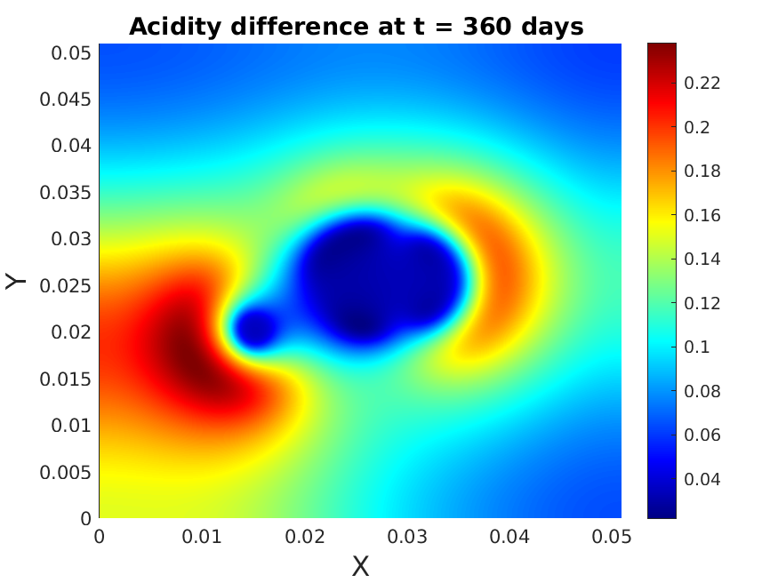
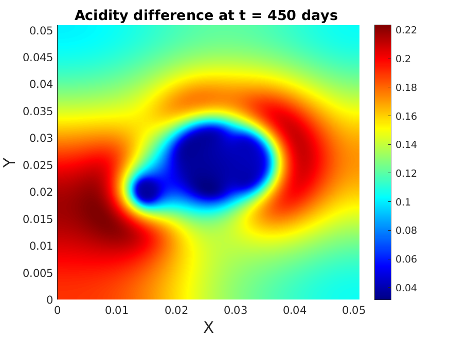

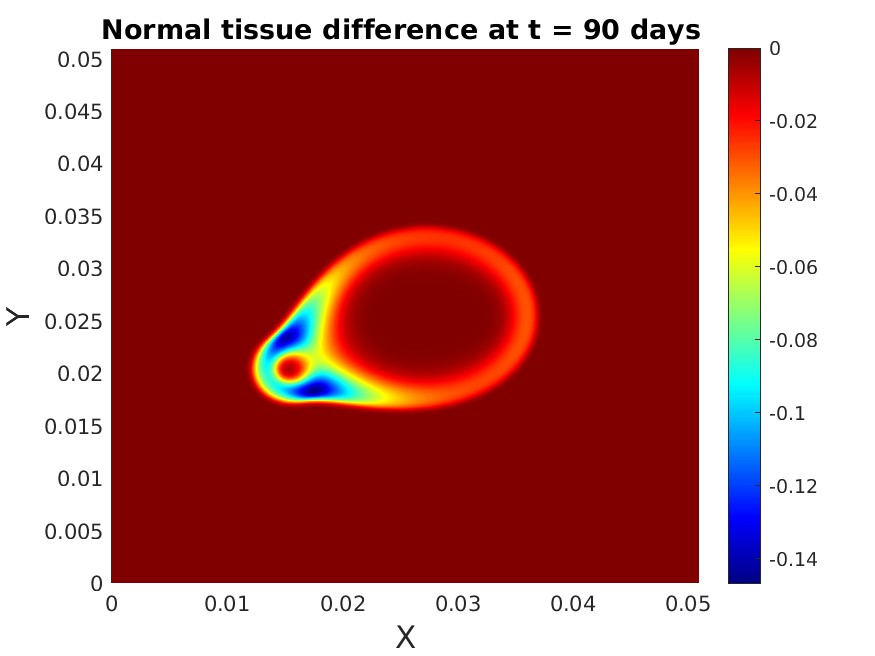
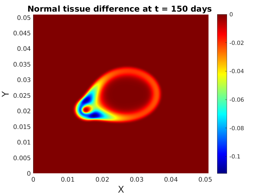
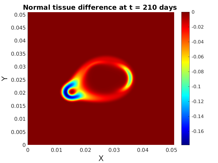
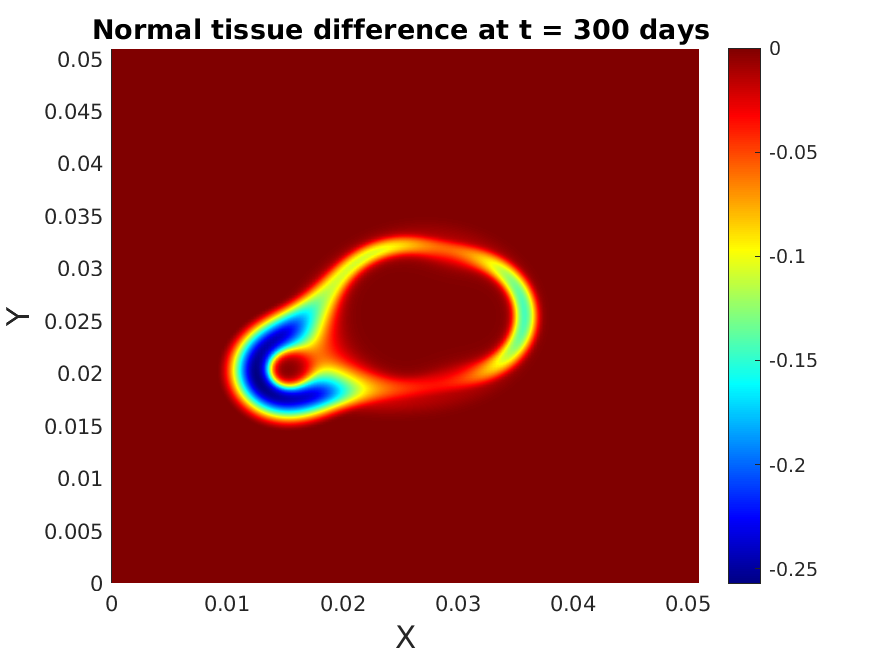
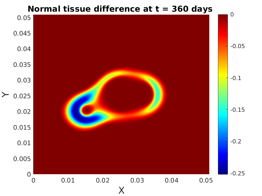
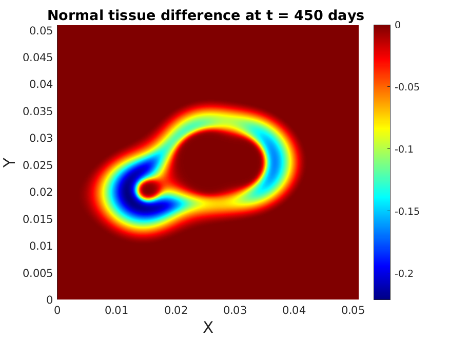

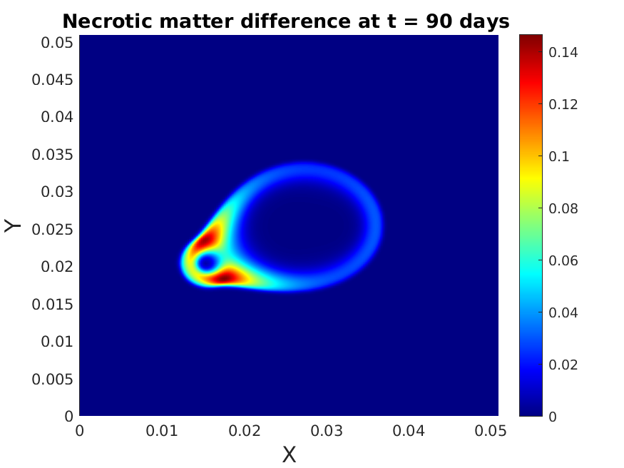

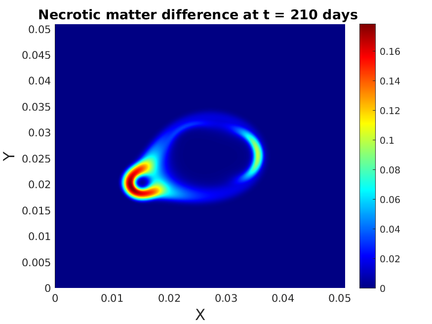
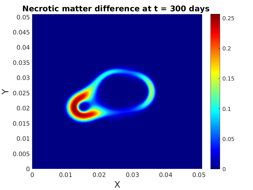
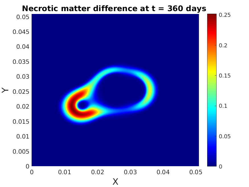
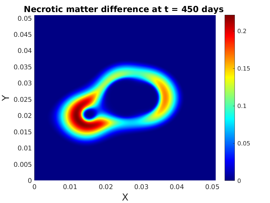
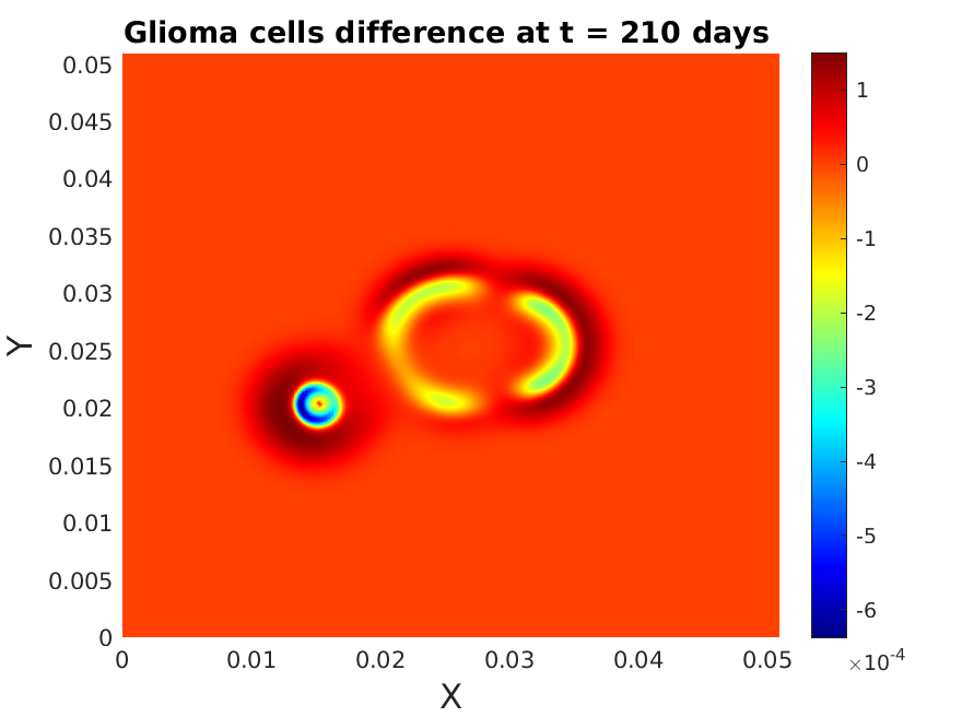
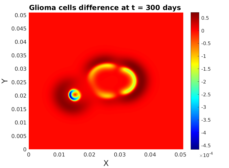
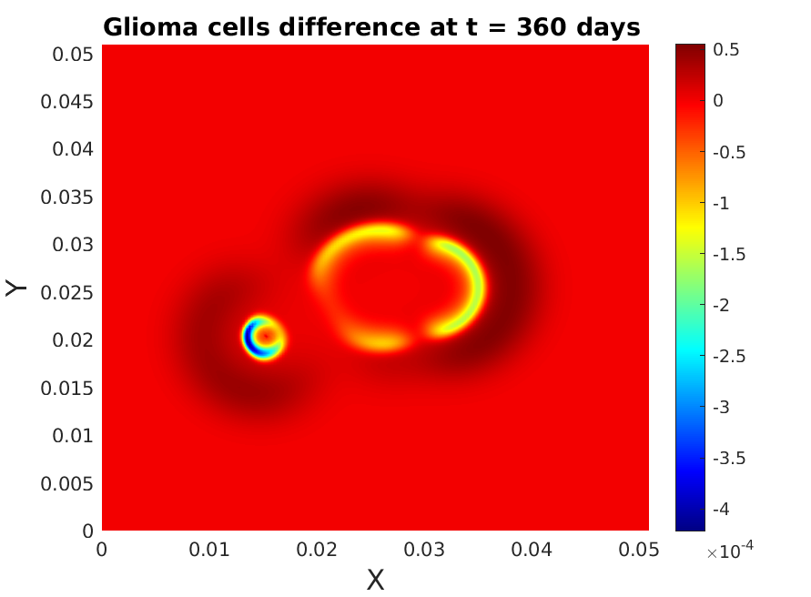
Finally, we also study the effect of drag coefficients in (3.9). Recall that they represent the resistance inferred by the phases in contact when passing over each other. They are contained in the diffusion and drift coefficients of system (3.50). In the computations for Figure 2 we had considered them to be different, more precisely . This ensured a relatively easy movement of glioma through normal tissue when compared to the shift over necrotic matter of both normal tissue and cancer cells. Now let all these drag coefficients be equal (as was assumed in [19]) and take the previously lowermost value , thus reducing the drag between necrotic matter and the other two phases. The differences between the two cases are plotted in Figure 4 and show in the second case an enhanced outward migration of glioma cells, away from the highly acidic area at the core of the pseudopalisade and with a pronounced suppression of normal cells, and emergence of larger necrotic matter. An opposite effect is noticed when letting , all at the previously highest value ; we do not show here those results (we refer for them to [25]), but rather illustrate in Figure 5 the situation when all drag coefficients equal the previously intermediate value . This means that the drag between cancer cells and normal tissue is increased, while they can easier shift over the necrotic matter. As a consequence, the extent of the pseudopalisades is reduced, but the glioma aggregates in the garland-like structures are larger. This is due not only to the higher drag between cancer cells and normal tissue, but also to the lower value, which ensures that the glioma cells can leave faster than previously the acidic area inside the ’ring’. Around the site where the cancer cells were initially more concentrated the necrosis is reduced and the normal tissue is better preserved.
Acknowledgement
P.K. acknowledges funding by the German Academic Exchange Service (DAAD) in form of a PhD scholarship.
30 days

90 days

150 days

210 days

300 days

360 days

450 days


30 days

90 days

150 days

210 days

300 days

360 days

450 days


Appendix
Non-dimensionalisation
Parameters
The following table summarises the parameters used in the simulations of Section 5.
| Parameter | Meaning | Value | Reference |
|---|---|---|---|
| acidity threshold for cancer cell death | mol/L | [38] | |
| proton production rate | mol /(Ls) | [27], [29] | |
| proton removal rate | /s | [26] | |
| acidity diffusion coefficient | m2/s | [27], [26] | |
| glioma growth/decay rate | /s | [35, 13] | |
| normal cells decay rate | /s | this work | |
| normal cells decay rate | /s | this work | |
| drag force coefficient between glioma and normal cells | N m-4s | this work | |
| drag force coefficient between normal and necrotic cells | N m-4s | this work | |
| drag force coefficient between glioma and normal cells | N m-4s | this work | |
| coefficient in the additional pressure on glioma due to acidity interaction | N m-2 L/mol | this work | |
| dimensionless coefficient in the additional pressure on normal cells due to glioma | 1 | this work | |
| coefficient in the additional pressure on normal cells due to glioma | N m-2 | this work | |
| coefficient in the additional pressure on glioma due to their crowding | N m-2 | this work |
References
- [1] J.C.L. Alfonso et al. “Why one-size-fits-all vaso-modulatory interventions fail to control glioma invasion: in silico insights” In Scientific Reports 6, 2016, pp. 37283
- [2] R. J. Atkin and R. E. Craine “Continuum theories of mixtures: basic theory and historical development” In The Quarterly Journal of Mechanics and Applied Mathematics 29.2, 1976, pp. 209–244 DOI: 10.1093/qjmam/29.2.209
- [3] C. Barbarosie “Representation of divergence-free vector fields” In Quarterly of Applied Mathematics 69.2 Brown University, 2011, pp. 309–316 URL: http://www.jstor.org/stable/43638978
- [4] Nicola Bellomo “Modeling Complex Living Systems” Birkhäuser Boston, 2008 DOI: 10.1007/978-0-8176-4600-4
- [5] Daniel J. Brat et al. “Pseudopalisades in Glioblastoma Are Hypoxic, Express Extracellular Matrix Proteases, and Are Formed by an Actively Migrating Cell Population” In Cancer Research 64.3 American Association for Cancer Research (AACR), 2004, pp. 920–927 DOI: 10.1158/0008-5472.can-03-2073
- [6] Daniel J. Brat and Timothy B. Mapstone “Malignant Glioma Physiology: Cellular Response to Hypoxia and Its Role in Tumor Progression” In Annals of Internal Medicine 138.8 American College of Physicians, 2003, pp. 659 DOI: 10.7326/0003-4819-138-8-200304150-00014
- [7] C.J.W. Breward, H.M. Byrne and C.E. Lewis “The role of cell-cell interactions in a two-phase model for avascular tumour growth” In Journal of Mathematical Biology 45.2 Springer ScienceBusiness Media LLC, 2002, pp. 125–152 DOI: 10.1007/s002850200149
- [8] H.M. Byrne, J.R. King, D.L.S. McElwain and L. Preziosi “A two-phase model of solid tumour growth” In Applied Mathematics Letters 16.4, 2003, pp. 567–573 DOI: https://doi.org/10.1016/S0893-9659(03)00038-7
- [9] Martina Conte and Christina Surulescu “Mathematical modeling of glioma invasion: acid- and vasculature mediated go-or-grow dichotomy and the influence of tissue anisotropy” In Applied Mathematics and Computation 407, 2021, pp. 126305 DOI: https://doi.org/10.1016/j.amc.2021.126305
- [10] G. Corbin et al. “Modeling glioma invasion with anisotropy- and hypoxia-triggered motility enhancement: From subcellular dynamics to macroscopic PDEs with multiple taxis” In Mathematical Models and Methods in Applied Sciences 31.01, 2021, pp. 177–222 DOI: 10.1142/S0218202521500056
- [11] Anne Dietrich, Niklas Kolbe, N. Sfakianakis and C. Surulescu “Multiscale modeling of glioma invasion: from receptor binding to flux-limited macroscopic PDEs” In arXiv: Tissues and Organs, 2020
- [12] Donald A. Drew and Stephen L. Passman “Theory of Multicomponent Fluids” In Applied Mathematical Sciences 135, Applied Mathematical Sciences New York, NY: Springer New York, 1999, pp. 324 DOI: 10.1007/b97678
- [13] S.E. Eikenberry et al. “Virtual glioblastoma: growth, migration and treatment in a three-dimensional mathematical model” In Cell Proliferation 42.4 Wiley Online Library, 2009, pp. 511–528
- [14] C. Engwer, T. Hillen, M. Knappitsch and C. Surulescu “Glioma follow white matter tracts: a multiscale DTI-based model” In Journal of Mathematical Biology 71.3 Springer, 2015, pp. 551–582
- [15] C. Engwer, A. Hunt and C. Surulescu “Effective equations for anisotropic glioma spread with proliferation: a multiscale approach and comparisons with previous settings” In Mathematical Medicine and Biology: an IMA Journal 33.4 Oxford University Press, 2015, pp. 435–459
- [16] C. Engwer, M. Knappitsch and C. Surulescu “A multiscale model for glioma spread including cell-tissue interactions and proliferation” In J. Math. Biosc. Eng. 13, 2016, pp. 443–460
- [17] Harald Garcke, Kei Fong Lam, Robert Nürnberg and Emanuel Sitka “A multiphase Cahn-Hilliard-Darcy model for tumour growth with necrosis” In Mathematical Models and Methods in Applied Sciences 28.03, 2018, pp. 525–577 DOI: 10.1142/S0218202518500148
- [18] A. Hunt and C. Surulescu “A Multiscale Modeling Approach to Glioma Invasion with Therapy” In Vietnam Journal of Mathematics 45.1-2 Springer ScienceBusiness Media LLC, 2016, pp. 221–240 DOI: 10.1007/s10013-016-0223-x
- [19] Trachette L. Jackson and Helen M. Byrne “A mechanical model of tumor encapsulation and transcapsular spread” In Mathematical Biosciences 180.1, 2002, pp. 307–328 DOI: https://doi.org/10.1016/S0025-5564(02)00118-9
- [20] A.F. Jones, H.M. Byrne, J.S. Gibson and J.W. Dold “A mathematical model of the stress induced during avascular tumour growth” In Journal of Mathematical Biology 40.6, 2000, pp. 473–499 DOI: 10.1007/s002850000033
- [21] Ansgar Jüngel “The boundedness-by-entropy method for cross-diffusion systems” In Nonlinearity 28.6, 2015, pp. 1963–2001 DOI: 10.1088/0951-7715/28/6/1963
- [22] Ansgar Jüngel and Ines Viktoria Stelzer “Entropy structure of a cross-diffusion tumor-growth model” In Math. Models Methods Appl. Sci. 22.7, 2012, pp. 1250009, 26 DOI: 10.1142/S0218202512500091
- [23] Paul Kleihues et al. “Histopathology, classification, and grading of gliomas” In Glia 15.3 Wiley, 1995, pp. 211–221 DOI: 10.1002/glia.440150303
- [24] Niklas Kolbe et al. “Modeling multiple taxis: Tumor invasion with phenotypic heterogeneity, haptotaxis, and unilateral interspecies repellence” In Discrete and Continuous Dynamical Systems - B 26.1, 2021, pp. 443–481
- [25] Pawan Kumar “Mathematical modeling of glioma patterns as a consequence of acidosis and hypoxia”, 2021
- [26] Pawan Kumar, Jing Li and Christina Surulescu “Multiscale modeling of glioma pseudopalisades: contributions from the tumor microenvironment” In J. Math. Biol. 82:49, 2021
- [27] Pawan Kumar and Christina Surulescu “A flux-limited model for glioma patterning with hypoxia-induced angiogenesis” In Symmetry 12.11 Multidisciplinary Digital Publishing Institute, 2020, pp. 1870
- [28] G Lemon and JR King “Multiphase modelling of cell behaviour on artificial scaffolds: effects of nutrient depletion and spatially nonuniform porosity” In Mathematical Medicine and Biology 24.1 Oxford University Press, 2007, pp. 57–83
- [29] G.R. Martin and R.K. Jain “Noninvasive Measurement of Interstitial pH Profiles in Normal and Neoplastic Tissue Using Fluorescence Ratio Imaging Microscopy” In Cancer Research 54.21 American Association for Cancer Research, 1994, pp. 5670–5674 URL: https://cancerres.aacrjournals.org/content/54/21/5670
- [30] A. Martínez-González, G.F. Calvo, L.A. Pérez Romasanta and V.M. Pérez-García “Hypoxic cell waves around necrotic cores in glioblastoma: a biomathematical model and its therapeutic implications” In Bulletin of Mathematical Biology 74.12 Springer, 2012, pp. 2875–2896
- [31] K. Painter and T. Hillen “Mathematical modelling of glioma growth: the use of diffusion tensor imaging (DTI) data to predict the anisotropic pathways of cancer invasion” In J. Theor. Biol. 323, 2013, pp. pp. 25–39
- [32] Luigi Preziosi and Andrea Tosin “Multiphase modelling of tumour growth and extracellular matrix interaction: mathematical tools and applications” In Journal of Mathematical Biology 58.4-5 Springer ScienceBusiness Media LLC, 2008, pp. 625–656 DOI: 10.1007/s00285-008-0218-7
- [33] Luigi Preziosi and Guido Vitale “A multiphase model of tumor and tissue growth including cell adhesion and plastic reorganization” In Mathematical Models and Methods in Applied Sciences 21.09, 2011, pp. 1901–1932 DOI: 10.1142/S0218202511005593
- [34] G Sciumè et al. “A multiphase model for three-dimensional tumor growth” In New Journal of Physics 15.1 IOP Publishing, 2013, pp. 015005 DOI: 10.1088/1367-2630/15/1/015005
- [35] A.M. Stein et al. “A mathematical model of glioblastoma tumor spheroid invasion in a three-dimensional in vitro experiment” In Biophysical Journal 92.1 Elsevier, 2007, pp. 356–365
- [36] Andrea Tosin and Luigi Preziosi “Multiphase modeling of tumor growth with matrix remodeling and fibrosis” In Mathematical and Computer Modelling 52.7, 2010, pp. 969–976 DOI: https://doi.org/10.1016/j.mcm.2010.01.015
- [37] Jahn O. Waldeland and Steinar Evje “A multiphase model for exploring tumor cell migration driven by autologous chemotaxis” In Chemical Engineering Science 191, 2018, pp. 268–287 DOI: https://doi.org/10.1016/j.ces.2018.06.076
- [38] B.A. Webb, M. Chimenti, M.P. Jacobson and D.L. Barber “Dysregulated pH: a perfect storm for cancer progression” In Nature Reviews Cancer 11.9 Springer ScienceBusiness Media LLC, 2011, pp. 671–677 DOI: 10.1038/nrc3110
- [39] F.J. Wippold et al. “Neuropathology for the Neuroradiologist: Palisades and Pseudopalisades” In American Journal of Neuroradiology 27.10 American Journal of Neuroradiology, 2006, pp. 2037–2041 URL: http://www.ajnr.org/content/27/10/2037
- [40] S.M. Wise, J.S. Lowengrub, H.B. Frieboes and V. Cristini “Three-dimensional multispecies nonlinear tumor growth—I” In Journal of Theoretical Biology 253.3 Elsevier BV, 2008, pp. 524–543 DOI: 10.1016/j.jtbi.2008.03.027