Leveraging Static Models for Link Prediction in Temporal Knowledge Graphs

Abstract

The inclusion of temporal scopes of facts in knowledge graph embedding (KGE) presents significant opportunities for improving the resulting embeddings, and consequently for increased performance in downstream applications. Yet, little research effort has focussed on this area and much of the carried out research reports only marginally improved results compared to models trained without temporal scopes (static models). Furthermore, rather than leveraging existing work on static models, they introduce new models specific to temporal knowledge graphs. We propose a novel perspective that takes advantage of the power of existing static embedding models by focussing effort on manipulating the data instead. Our method, SpliMe, draws inspiration from the field of signal processing and early work in graph embedding. We show that SpliMe competes with or outperforms the current state of the art in temporal KGE. Additionally, we uncover issues with the procedure currently used to assess the performance of static models on temporal graphs and introduce two ways to counteract them.

1 Introduction

A knowledge graph (KG) is a graph used for representing structured information about the world, which can then be utilized in tasks such as question answering [11], relation extraction [3] and recommender systems [10]. Information is stored in the form of (subject, predicate, object) triples, e.g., (Obama, presidentOf, USA), also called facts. The subject and object are also referred to as entities. In the graph representation, the entities are nodes and predicates are the labelled directed edges between them.

Knowledge graph completion is the problem of inferring missing facts in a KG. This is often achieved through KG embedding where the entities and predicates making up the KG are embedded into a low-dimensional vector space. The embedding models implement scoring functions to calibrate the positions of entities and predicates in the vector space. A number of different scoring functions have been proposed in order to successfully capture the underlying structure of a static KG. Surveys of these models can be found in [12, 21].

A largely unexplored component of KG embedding is the inclusion of the temporal scopes of facts–the time at which a fact occurred or held true. Referring back to our earlier example: Obama was only president of the USA from 2009 to 2017. Alternatively, there exist event KGs where each event is associated with a timestamp (e.g. (Obama, awarded, noble-peace-prize, 2015)). Both are collectively referred to as temporal knowledge graphs (TKG).

It is known that including temporal scopes of facts in a KG embedding would result in improved performance [6, 9, 27]. However, comparatively little research has been performed in this area. The performance results of which are only marginally better than that reported by models without temporal scopes. Furthermore, these approaches focus on introducing new models specific to temporal graphs rather than finding ways to leverage the impressive performance of existing static models. We believe that the option of transforming the data (e.g., through splitting) to achieve this has been overlooked.

We propose a new method called SpliMe  which operates on the graph in order to leverage the power of static embedding models. Specifically, SpliMe uses the valid times (temporal scopes) of facts to embed predicates in three different ways: (i) timestamping, (ii) splitting (leverages change point detection [2]), and (iii) merging. Similarly to [9], SpliMe is model agnostic, meaning it can be used with any existing static embedding model and therefore take advantage of further development in this area. The core of SpliMe is a transformation function which maps a TKG into a new representation where the temporal scope is included at the level of entities and/or predicates. The resulting KGs can subsequently be embedded using models for static KGs. We carried out several experiments and compared SpliMe with state-of-the-art TKG embedding models. Despite only performing experiments with TransE, a conceptually simple model, results show that SpliMe outperforms most of these models. We believe that the results can be increased by using more expressive static embedding models such as ComplEx [24] or SimplE [15].

Additionally, we uncover issues with the procedure used to evaluate static models on temporal knowledge graphs. Specifically, the current procedure causes test-leakage, i.e., elements from the test set appear in the training set. Due to this, the performance of static models in this scenario is sometimes overestimated. Consequently, the relative increase in performance that temporal models provide is underestimated. We provide two procedures that fix this error and show even with this fix, SpliMe still matches or outperforms its competitors.

2 Preliminaries

Given an entity set $\mathcal{E}=\{e_{1},e_{2},\dots,e_{n}\}$ and a predicate set $\mathcal{P}=\{r_{1},r_{2},\dots,r_{m}\}$, a knowledge graph $G$ is a set of observed triples, i.e., $G=\{(s,p,o)\ |\ s\in\mathcal{E},\ p\in\mathcal{P},\ o\in\mathcal{E}\}$. In the graph representation, entities are nodes and predicates are labelled directed edges between them. Temporal knowledge graphs (TKGs) also include a temporal scope for (a subset of)) facts. Time in this case is modeled as a set of discrete, linearly ordered timestamps: $\mathcal{T}=\{t_{1},t_{2},\dots,t_{l}\}$. TKGs come in two varieties: the first is as a set of quadruples, i.e. $\mathit{T}=\{(s,p,o,h)|h\in\mathcal{T}\}$ where $h$ is a timestamp to denote when the fact happened. This method is useful for modelling the occurrences of events. A TKG defined in this manner is also called an event TKG. The second variety is as a set of quintuples, i.e., $T=\{(s,p,o,b,e)\ |\ b,e\in\mathcal{T},b\leq e\}$. This formulation models the time period temporal scope during which facts held true, also known as valid time TKG.

We introduce some notations that will be used throughout the paper. We consider the subgraph $T^{p=r}$ to denote all facts in a TKG containing the predicate $r\in\mathcal{P}$, i.e., $T^{p=r}=\{(s,p,o,b,e)\in T\ |\ p=r\}$. Analogously, we define $T^{s=z}$ as all facts containing entity $z\in\mathcal{E}$, $T^{b=t}$ as all facts with start time $t\in\mathcal{T}$ and so on. This indexation can be chained: $T^{p=r,e=t}$ is the TKG containing all facts which contain predicate $r$ and end at timestamp $t$.

Knowledge graph embedding

is the representation of a KG in a continuous, low-dimensional vector space by learning a vector representation for each entity and predicate. The vectors represent the latent features of entities and relationships: the underlying parameters that determine their interactions. For a triple ($s,p,o$), let ($e_{s},e_{p},e_{o}$) denote its embedding vectors. Taking a KG and a random initialization of the vectors as an input, a vector representation of the KG is gradually learned using a scoring function $\phi(s,p,o)$. The scoring function should reflect how well the embedding captures the semantics of the KG. For instance, the scoring function of TransE, as explained in further detail in Section 0.E.1, is written as $\phi(s,p,o)=||e_{s}+e_{p}-e_{o}||_{1,2}$. The learned embeddings can be used in tasks such as classification, clustering, and link prediction. In this work, we are focussed on the last.

Link prediction

is the task of predicting the most likely element given a tuple where one element is missing, e.g., given a triple (s,p,?), to predict the most likely $o\in\mathcal{E}$. With SpliMe we introduce a novel approach that facilitates temporally aware link prediction using static embedding methods. That is, we take the temporal scope of facts into account when performing link prediction. To achieve this, SpliMe transforms every (s,p,o,h) tuple into an approximately equivalent ($s,p\text{(}h\text{)},o$) triple, where the specific predicate used is a function of time.

Network proximity measures

capture the proximity or similarity between a pair of nodes in a graph. In order to do this, two sources of information can be used: the structure of the graph itself or the attributes of the nodes. As KGs do not have node or predicate attributes, we use methods based solely on the structure of the graph. This approach has the advantage that it works for any type of KG. In contrast, an attribute based approach requires a similarity function to be defined for each attribute type. To be precise, we utilize measures based on node-neighborhoods. The node-neighborhood of a node, or entity $s\in\mathcal{E}$, denoted $\Gamma(s)$, is the set of nodes that are direct neighbors of $s$. The idea is that two nodes are more likely to form a link if they have many overlapping neighbors. We experiment with three network proximity measures. Jaccard, Adamic/Adar, and Preferential attachment. Their formulations are written as a function $sim(s,o)$ of the entity pair being evaluated as shown below:

Jaccard	Adamic/Adar	Pref. attachment
$sim(s,o)=\frac{|\Gamma(s)\cap\Gamma(o)|}{|\Gamma(s)\cup\Gamma(o)|}$	$\sum\limits_{z\in\Gamma(s)\cap\Gamma(o)}\ \frac{1}{\log|\Gamma(z)|}$	$|\Gamma(s)|*|\Gamma(o)|$

The first measure is the well known Jaccard set similarity metric. The second measure Adamic/Adar was introduced in [1] based on the notion that common features (nodes) should be weighted less heavily than uncommon ones. Lastly, preferential (pref.) attachment argues that the probability that a node obtains a new edge is proportional to its current number of edges. In this paper, we use the proximity scores over time as a measure of graph evolution. By considering the proximity scores between entities over time as time series data, we can evaluate when their semantics change significantly. This is done through change point detection.

Change point detection (CPD)

is the problem of finding (abrupt) variations (change points) in time series data [2]. Recall that the timestamp set $\mathcal{T}$ contains $l$ elements. CPD considers a time series $S$, i.e., $S=\{x_{1},x_{2},\dots,x_{l}\}$, where $x_{i}$ is a data vector designating the value of the time series at timestamp $i$ with $1\leq i\leq l$. In our case, we create a time series for every predicate $r$, i.e., we create $S_{r}\ \forall r\in\mathcal{P}$. For a given $S_{r}$, each entry $x_{i}$ represents a vector containing similarity scores between nodes that are connected via edges labeled with $r$ at some timestamp $i$.

Truong et al. [25] define CPD as a model selection problem which consists of selecting the best possible segmentation of $S$ such that an associated cost function is minimized. In this definition a CPD algorithm consists of three components: a cost function, a search method and a constraint (on the number of change points). The cost function is a measure of homogeneity, i.e., how similar data points in a given segment are. The search method concerns locating possible segment boundaries, i.e., it locates parts of the signal that should be grouped together. When the number of change points is not known a priori a complexity penalty is applied to prevent overfitting to the data. The larger the number of change points, the higher the induced penalty. In addition, let $c(\cdot)$ denote a cost function which measures how good a fit is for a sub-signal of the signal $S$. Commonly used cost functions are the $\ell_{1}$ and $\ell_{2}$ norms. However, these can only be used when the data exists in a euclidean space. In other cases, one prefers a kernel function [8]. Since we apply CPD to the output of network proximity measures, whose outputs do not necessarily occupy a euclidean space, SpliMe uses the well-known radial basis kernel function instead. For a further explanation of CPD and how it relates to SpliMe, including a full explanation of the cost function used, we refer to Section 0.D in the Appendix.

More formally, CPD is defined as finding an optimal segmentation $L=\{k_{1},\ldots,k_{K}\}$, $0\leq K\leq l\in\mathbb{N}^{+}$ for $S$, i.e., $L$ is a set of indices of elements of $S$ at which change points occur. In turn, $\textit{pen}(L)$ measures the complexity associated with the segmentation. Let $S_{a,b}$ denote the sub-signal of $S$ between indices $a,b\in\mathcal{T},a\leq b$. The CPD problem for an unknown number of change points can be written as

$\leavevmode\nobreak\ \leavevmode\nobreak\ \leavevmode\nobreak\ \leavevmode\nobreak\ \leavevmode\nobreak\ \leavevmode\nobreak\ \leavevmode\nobreak\ \leavevmode\nobreak\ \leavevmode\nobreak\ \leavevmode\nobreak\ \leavevmode\nobreak\ \leavevmode\nobreak\ \leavevmode\nobreak\ \leavevmode\nobreak\ \leavevmode\nobreak\ \leavevmode\nobreak\ \leavevmode\nobreak\ \leavevmode\nobreak\ \leavevmode\nobreak\ \leavevmode\nobreak\ \leavevmode\nobreak\ \leavevmode\nobreak\ \leavevmode\nobreak\ \leavevmode\nobreak\ \leavevmode\nobreak\ \leavevmode\nobreak\ \leavevmode\nobreak\ \leavevmode\nobreak\ \leavevmode\nobreak\ \leavevmode\nobreak\ \min\limits_{L}\sum_{k=1}^{K-1}c(S_{k,k+1})+\textit{pen}(L).$

In our experiments, we use the bottom-up search function. This procedure starts with many change points and then deletes those that are less significant. This method has two parameters. The first is minimum size, which specifies the minimum length of a segment. The second is jump, which specifies how many samples apart the initial change points should be distributed.

3 SpliMe

We propose SpliMe as a way to include the temporal scope of facts at the level of entities and/or predicates. At the core of SpliMe is a transformation function $f\ :\mathit{T}\mapsto\mathit{T}^{\prime}$, which takes a TKG and returns a new TKG where temporal scope is (partially) included at the level of entities and/or predicates. $f$ is then applied repeatedly until a stopping criterion is met. While SpliMe can be applied to both entities and predicates, preliminary research showed that it works best when applied to the latter. Therefore, we will focus on the results on predicates for this paper. We have developed several different implementations for $f$ categorized into timestamping, splitting and merging approaches. In the coming sections we will provide an in-depth explanation of each approach. Additionally, we provide an algorithm for each method. Due to space constraints, only the algorithm for the CPD-based efficient splitting method is given here, the others are available in the Appendix 0.B.

3.1 Timestamping

Conceptually the simplest approach, timestamping converts each temporal fact in the TKG into a set of facts, one for each timestamp for which the fact was true. A variant of this approach was previously defined in [18] under the name Naive-TTransE. Formally, given an injective function $u(\mathcal{P},\mathcal{T})\mapsto\mathcal{P}^{\prime}$ which creates a new predicate for every (predicate, timestamp) combination, timestamping creates a set of facts for a given quintuple, i.e. $f(s,p,o,b,e)=\{(s,u(p,t),o)\ |\ \forall t\in\mathcal{T}\ s.t.\ b\leq t\leq e\}$. To obtain a fully timestamped KG, this process must be applied to every fact in a TKG.

3.2 Splitting

Timestamping serves mostly as a baseline method for including the temporal scope of facts to which we can compare our other implementations. The creation of a large number of triples and predicates may cause the resulting KG to become too sparse. As an alternative, we introduce two different approaches: splitting and merging. In this section we firstly discuss the common splitting framework, before displaying our two different splitting approaches. In the next section we will discuss the merging approach. Given a predicate $r\in\mathcal{P}$ and a timestamp $t\in\mathcal{T}$, splitting adds two new predicates, $r_{1}$ and $r_{2}$, to the predicate set $\mathcal{P}^{\prime}=\{r_{1},r_{2}\}\cup\mathcal{P}$. Each quintuple $(s,p,o,b,e)\in T^{p=r}$ is then updated to contain either $r_{1}$ if $e\leq t$, or $r_{2}$ if $b\geq t$. Otherwise, the fact is split into two: $\{(s,r_{1},o,b,t),(s,r_{2},o,t,e)\}$. As a result, splitting does not necessarily increase the size of the dataset. Instead, splitting reduces the number of facts associated with each predicate.

Parameterized splitting

Formally, parameterized splitting is done via a function $f:(\mathit{T},c_{p},c_{t})\mapsto\mathit{T}^{\prime}$, which given a TKG $\mathit{T}$, splitting criteria $c_{p}$ which selects a predicate, and criteria $c_{t}$ which selects a timestamp, maps to a new TKG $\mathit{T}^{\prime}$. The challenge here lies in defining an effective $c_{p}$ and $c_{t}$. For $c_{p}$, a general approach that produced a good performance in our experimental evaluation is selecting the predicate that occurs the most, i.e.,

$$c_{p}=\arg\max_{r\in\mathcal{P}}|\mathit{T}^{p=r}|.$$

Intuitively, this is the predicate that benefits the most by making it more specific. We propose two methods for $c_{t}$: time and count. Let $t_{f}^{r}$ and $t_{l}^{r}$ denote the first and last timestamps associated with a predicate $r\in\mathcal{P}$ in a TKG. The time method splits a fact that contains $r$ at $t=(t_{f}^{r}+t_{l}^{r})/2$. The count method selects a point in time that results in the most balanced number of triples on both sides of the split. This is done by counting how many facts end before, or end after a specific timestamp. Formally, the count function can be written as

$$c_{t}(r)=\arg\min_{t\in\mathcal{T}}abs(|\mathit{T}^{p=r,e\leq t}|-|T^{p=r,b\geq t}|),$$

where abs denotes the absolute value function. Furthermore, we require that $T^{p=r,e\leq t}\neq\emptyset$ and $\mathit{T}^{p=r,b\geq t}\neq\emptyset$ in order to prevent the consideration of non-existing (predicate, timestamp) combinations. We have performed experiments with both methods and found that both achieve similar results. Which one performs best depends on the dataset used. Regarding stop condition, we continue splitting until the number of predicates in the KG has grown by a factor $Grow$.

CPD-based efficient splitting

The parameterized splitting method described above uses relatively simple measures to decide where, and when, to apply splits. However, there is much more information present in the structure of the KG that could be used to inform the splitting procedure. Thus, we introduce CPD-based efficient splitting: a two-step process to determine how to place split points.

In the first step, network proximity measures are applied to a TKG to calculate a signature vector for every predicate, at every timestamp, i.e., we create a time series $S_{r}$, $\ \forall r\in\mathcal{P}$. For any $S_{r}$, each entry represents a vector of proximity scores between pairs of nodes that are connected by $r$ in the graph. The sequence of entries then represents how the predicate has evolved over time. The second step is to input these vectors to a CPD algorithm. Split points are placed at the timestamps where CPD algorithm has identified change points.

To overcome sparsity of information, a TKG is considered as an undirected graph, i.e., we do not take into account whether entities occur as subjects or objects. Signatures are created by slicing the TKG into subgraphs representing the different (predicate, timestamp) combinations, i.e., a subgraph $s_{r,t}=\mathit{T}^{p=r,b\leq t\leq e}$ is created for every $(r,t)$ pair.

Let $f_{score}:(\mathcal{E},\mathcal{E},\mathit{T})\mapsto$ denote a proximity function (e.g. preferential attachment) that calculates the proximity score for a given entity pair on the given subgraph $s_{r,t}$. Additionally, let $\textit{pairs}_{r}$ denote the set of entity pairs for predicate $r$, i.e., $\textit{pairs}_{r}=\{(e_{1},e_{2})\ |\ e_{1},e_{2}\in\mathcal{E}\wedge((e_{1},p,e_{2})\lor(e_{2},p,e_{1})\in\mathit{T}^{p=r})\}$. Now, for every predicate $r$ we calculate the proximity score of each pair in $\textit{pairs}_{r}$ for every timestamp and add the result to the signature vector. That is, we calculate $f_{score}(e_{1},e_{2},s_{r,t})\ \forall(e_{1},e_{2})\in pair_{r}$ and $\ \forall t\in\mathcal{T}$.

Next, we discuss how CPD is applied to the signature vectors. As the number of change points for a given predicate is unknown, a complexity penalty or residual value has to be used to determine the optimal number of split/change points. In our experimental evaluation, we utilize a bottom-up segmentation algorithm in combination with a residual $\epsilon$ in the range [1, 100] depending on the data being transformed. A high $\epsilon$ residual allows for more leeway in reconstructing the data, necessitating less change points. Vice-versa, a low value for $\epsilon$ implies more change points. To ensure that the found change points do not depend on the magnitude of the signatures, we normalize all signatures before passing them into the CPD algorithm.

1:function cpd_split($\mathit{T}$, $\mathcal{P}$, $f_{score}$)

2:     split_points $\leftarrow$ {} $\triangleright$ Stores a list of splits for every predicate.

3:     for all $r\in\mathcal{P}$ do

4:         $\mathit{T}^{\prime}$ $\leftarrow$ $\mathit{T}^{p=r}$

5:         signatures $\leftarrow$ $\textsc{calc\_signatures}(\mathit{T}^{\prime},f_{score})$

6:         $\textit{split\_points}_{p}$ $\leftarrow$ $\textit{apply\_cpd}(\textit{signatures})$

7:     end for

8:     $\mathcal{T}^{\prime\prime},\mathcal{P}^{\prime}$ $\leftarrow$ $\textit{apply\_split}(\mathit{T},\mathcal{P},\textit{split\_points})$ $\triangleright$ Each split point can be applied using the logic explained in Section 3.2.

9:return $\mathcal{T}^{\prime\prime},\mathcal{P}^{\prime}$

10:

11:function calc_signatures($\mathit{T}$, $f_{score}$)

12:     signatures $\leftarrow$ {} $\triangleright$ Stores a signature for every timestamp

13:     for all $t\in\mathcal{T}$ do

14:         $\mathit{T}^{\prime}$ $\leftarrow$ $\mathit{T}^{b\leq t,e\geq t}$ $\triangleright$ Slice the TKG to contain just the facts that are valid at $t$

15:         for all $(s,p,o,b,e)\in\mathit{T}^{\prime}$ do

16:              score $\leftarrow$ $f_{score}(s,o,\mathit{T}^{\prime})$

17:              $\textit{signatures}_{t_{s,o}}$ $\leftarrow$ score $\triangleright$ Store the score in the signature

18:         end for

19:     end for

20:return signatures

Algorithm 1 : SpliMe: CPD-based efficient splitting

Pseudocode for this approach is given in Algorithm 1. We have included two functions: one to calculate the signature vectors for a given predicate, and one which uses these signatures to calculate the split points and apply them. The main entry point for the procedure is the cpd_split function defined on line 1. The apply_cpd and apply_split procedures are not included for legibility. Firstly, a dictionary or hash set is created which will keep track of all the split points of a given predicate, for every timestamp (on line 2). Between lines 3 and 7 we loop over all predicates, slice the KG (line 4) calculate the signatures using $f_{score}$ (line 5). In the last line of the loop we perform CPD (line 6). Once all the predicates have been processed, we apply the found split points to the TKG and the predicate set (line 8). A new TKG and predicate set are returned on line 9.

Signature creation is done as follows. On line 13 we loop over all timestamps in the KG. In every loop we select only the facts that are valid at the given timestamp (line 14). We then loop over all these facts, calculate the proximity score of the entities it is composed of (line 16) and add that score to the signature vector (line 17). Because we model the evolution of node proximity over time, the location of each entry in the signature vector must be consistent. Therefore, we assume that adding to the signature always places an (s,o) pair at the same index.

3.3 Merging

The splitting methods described above refine the temporal scope of the the predicates in the knowledge graph at every iteration by making them more specific. They can therefore be considered top-down approaches. As an alternative we envision a bottom-up approach where, starting with a large selection of possible (predicate, timestamp) combinations, refinement is performed by selectively combining pairs. We will now describe such a method called merging.

Merging starts with a timestamped TKG (consisting of $(s,p,o,h)$ quadruples) and selectively merges predicates which belong to the same original predicate and are subsequent (or contiguous) in time. Given a predicate pair $(r_{a},r_{b})$ to merge, a new predicate $r_{c}$ is generated, and every $(s,p,o,h)\in\{\mathit{T}^{p=r_{a}}\cup\mathit{T}^{p=r_{b}}\}$ is then updated to contain $r_{c}$; lowering the number of unique predicates. By iteratively applying the merging procedure until no more merging candidates exist, one could regenerate the original graph. However, experimental results show that the performance declines when too many predicates are removed.

To select the predicates and timestamps that can be merged, we define two functions. A function $l_{p}:\mathcal{P}^{\prime}\mapsto\mathcal{P}$ which given a predicate of the timestamped TKG returns the source predicate in the original TKG, and a function $l_{t}:\mathcal{P}^{\prime}\mapsto\mathcal{T}$ which given a predicate of the timestamped TKG returns the time associated with that predicate. A predicate pair $(r_{a},r_{b})$ is only valid as a merge candidate if i) the source predicates are the same: $l_{p}(r_{a})=l_{p}(r_{b})$, and if ii) there exists no predicate whose timestamp is in between those associated with $r_{a}$ and $r_{b}$: $\nexists r_{c}\in\mathcal{P}^{\prime}\ s.t.\ l_{t}(r_{a})\leq l_{t}(r_{c})\leq l_{t}(r_{b})$. We continue this procedure until the number of predicates in the KG has shrunk by a factor $shrink$ compared to that in the timestamped KG.

4 Empirical Evaluation

In order to evaluate the effectiveness of SpliMe we have implemented the aforementioned methods and executed them on three TKGs commonly used for the evaluation of TKG embedding methods. In addition to this quantitative analysis, we have performed a qualitative analysis of SpliMe  which is available in the Appendix 0.C. All SpliMe methods were implemented in the Python programming language. Additionally, we use the Ruptures library [25] for change point detection. All models were trained using the Ampligraph framework, a suite of machine learning tools used for supervised learning [5].

4.1 Datasets

Experiments were performed on 3 datasets commonly used in TKG embedding literature. An overview of their characteristics is displayed in Table 1. We maintain the original train/test/validation splits for all datasets.

Wikidata12k & YAGO11k

are valid-time TKGs used in [6]. The temporal scopes are set to year-level granularity. For many facts in the data either the beginning or end time is missing. Here, the missing time is set to the first or last timestamp in the TKG respectively. Additionally, there are facts whose temporal scope is invalid either because they cannot be parsed correctly or because the end time is before the start time. These facts are removed. Both of these modifications are default procedure for handling these data sets.

ICEWS14

is an event-based TKG consisting of timestamped political events. It contains all events that occurred in 2014 and was extracted from the complete ICEWS KG by [7]. Because SpliMe operates on quintuples rather than quadruples, ICEWS14 is first converted into the valid-time format by setting $b=e=h$ for every fact.

Table 1: Overview of the characteristics of the used datasets.

Dataset	$|\mathcal{E}|$	$|\mathcal{P}|$	$|\mathcal{T}|$	$|\textit{train}|$	$|\textit{valid}|$	$|\textit{test}|$
YAGO11k	10,526	10	59	16,408	2,050	2,051
Wikidata12k	12,554	24	70	32,497	4,062	4,062
ICEWS14	7,128	230	365	72,826	8,941	8,963

4.2 Baselines

We compare the results of our methods with two baselines. The first is the Vanilla baseline as discussed in Section 5. This method strips out all temporal scopes from the TKG, turning it into a static KG. The second is the Random baseline which works by applying splits randomly across predicates and timestamps in a uniform manner. Specifically, at every split step, a predicate is chosen from the currently existing predicates. Then, a timestamp between that predicates first and last occurrence in the dataset is chosen. This is repeated until the desired number of predicates have been created. For the valid time TKGs we report the average of 7 runs. For ICEWS14 the results are averaged over 5 runs. Additionally, we compare SpliMe to the current state of the art: ATiSE [27], HyTE [6], TTransE [13], and TDG2E [23] for the valid-time TKGs, and ATiSE, DE-SimplE [9], HyTE, TA-DistMult [7] and TNT-ComplEx [17] for the event-based TKGs.

4.3 Hyperparameters

While SpliMe is model-agnostic and can be combined with any KG embedding method, we use TransE in our experiments and compare with TKG embedding models that are mostly built on top of the TransE family. Our model hyperparameters are adapted from [7]. We use the same model hyperparameters for all experiments. Specifically, we train for 200 epochs with embedding size = 100 and learning rate = $10^{-3}$. We set the batch size to 500 and generate 500 negative samples per batch. Optimization was done using the ADAM optimizer in combination with a self-adversarial loss function [16]. For CPD-based splitting, we use a kernelized mean change cost function with bottom-up search where jump size and minimal section length are both set to 1.

Because SpliMe  applies transformations to TKGs, we also have data hyperparameters. For both the time and count splitting methods we experimented with $Grow\in\{5,10,15,20,25,30\}$ for all data sets. Regarding merging, we tested $Shrink\in\{1.5,2,4,6,8,10\}$. Lastly, CPD-based splitting was evaluated using the Jaccard, Adamic/Adar (Adar) and Preferential attachment (Pref) proximity measures, with $\epsilon$ (residuals) $\in\{1.25,2.5,5,10,15,20\}$ for Wikidata12k and YAGO11k, and $\epsilon\in\{5,12.5,25,50,100,150,200\}$ for ICEWS14.

4.4 Evaluation Procedure

KG embeddings are evaluated on the link prediction task as described in [4]. For a triple in the test set (s,p,o) either the subject or object is replaced with all $e\in\mathcal{E}$. That is, subject and object evaluation is combined. In line with the filtered setting, we remove any resulting triples which occur in the train, test or validation sets. All created triples are then scored by the model and the result is sorted. The rank of the original triple is recorded. This process is repeated for all triples, giving us a set of ranks $R$. From this set we calculate two metrics. These are mean reciprocal rank (MRR) and hits@k for $k\in\{1,3,10\}$. These are defined as:

MRR	Hits@k
$\frac{1}{|R|}\sum_{h\in R}\frac{1}{h}$	$\frac{1}{|R|}\sum_{h\in R}\begin{cases}1\ \text{if}\ h\leq k\\ 0\ \text{otherwise}\end{cases}$

Finally, all results are obtained using the inter filter setting as described in Section 5.

4.5 Results

Table 2: Overview of the optimal result obtained for each method. The best results are highlighted in bold.

(a) Wikidata12k

Method	Setting	MRR	Hits@1	Hits@3	Hits@10	# Preds
Vanilla	-	0.209	12.4%	22.7%	37.9%	24
Random	-	0.289	17.9%	33.3%	50.7%	423
Timestamp	-	0.340	21.1%	40.8%	58.1%	1622
Split (time)	$\textit{Grow}=10$	0.320	20.1%	37.2%	54.9%	240
Split (count)	$\textit{Grow}=25$	0.300	18.3%	34.5%	53.8%	600
Split (CPD)	Pref, $\epsilon=2.5$	0.328	20.9%	38.1%	56.0%	726
Merge	$\textit{Shrink}=4$	0.358	22.2%	43.3%	61.0%	423

(b) YAGO11k

Method	Setting	MRR	Hits@1	Hits@3	Hits@10	# Preds
Vanilla	-	0.188	8.2%	23.8%	35.6%	10
Random	-	0.197	7.8%	25.2%	39.9%	200
Timestamp	-	0.197	6.9%	26.0%	41.2%	570
Split (time)	$\textit{Grow}=20$	0.213	9.0%	27.0%	43.2%	200
Split (count)	$\textit{Grow}=25$	0.196	8.1%	24.1%	40.3%	250
Split (CPD)	Pref, $\epsilon=5$	0.214	6.5%	29.9%	45.8%	177
Merge	$\textit{Shrink}=2$	0.195	6.2%	26.3%	42.0%	290

(c) ICEWS14

Method	Setting	MRR	Hits@1	Hits@3	Hits@10	# Preds
Vanilla	-	0.141	0.1%	18.9%	42.2%	230
Random	-	0.172	2.0%	23.4%	48.1%	3500
Timestamp	-	0.213	4.7%	29.4%	54.4%	17061
Split (time)	$\textit{Grow}=20$	0.190	3.0%	26.3%	51.6%	4600
Split (count)	$\textit{Grow}=25$	0.191	3.0%	26.2%	52.2%	5750
Split (CPD)	Adar, $\epsilon=25$	0.196	2.9%	27.3%	53.0%	5866
Merge	$\textit{Shrink}=1.5$	0.207	4.1%	28.7%	53.9%	11449

The best results displayed in Table 2 show that all methods, even the random baseline, provide an increase in performance on all metrics compared to the vanilla baseline. Therefore, we can say that incorporating time at the level of predicates improves the link prediction capabilities of static KGE models. Furthermore, all SpliMe methods have improved performance compared to the random baseline, suggesting that they indeed capture the temporal scope of facts in a more efficient manner.

On Wikidata12k the best result is achieved using the merge method creating a version of the dataset with 423 predicates (17.6 times increase). Here, merging outperforms all other approaches on every recorded metric. It outperforms Vanilla/TransE and the random baseline by approximately 23% and 10% on the hits@10 respectively. This represents a 60% and 20% increase in performance respectively.

On YAGO11k the best result is achieved using CPD in combination with preferential attachment as a proximity function. Notably, this method produces 177 predicates (17.7 times increase), which are 113 and 23 fewer than the best merge and split approaches respectively. CPD-based splitting outperforms the vanilla baseline by more than 10% on the hits@10, which is a 28% increase in performance.

Lastly, on ICEWS14 the best result is achieved with the timestamping approach, which achieves the highest scores on all metrics. Timestamping outperforms the random baseline by 6% (13% increase) on the hits@10. On the hits@1 metric, the difference is 2.7%, representing a 135% increase. Compared to our vanilla TransE baseline the results are better, especially on hits@1 as the vanilla baseline scores just 0.1%.

Table 3: Comparison of the best SpliMe approach, for each dataset, and the current state of the art. Best results are highlighted in bold. The method column contains the model name along with the paper that result was reported in.

(a) On Wikidata12k, the best SpliMe result was achieved with the merge method. On YAGO11k, the best SpliMe result was achieved using CPD-based splitting.

	Wikidata12k				YAGO11k
Method	MRR	Hits@1	Hits@3	Hits@10	MRR	Hits@1	Hits@3	Hits@10
SpliMe	0.358	22.2%	43.3%	61.0%	0.214	6.5%	29.9%	45.8%
ATiSE [27]	0.252	14.8%	28.8%	46.2%	0.185	12.6%	18.9%	30.1%
HyTE [27]	0.180	9.8%	19.7%	33.3%	0.105	1.5%	14.3%	27.2%
TTransE [27]	0.172	9.6%	18.4%	32.9%	0.108	2.0%	15.0%	25.1%
TDG2E [23]	-	-	-	40.2%	-	-	-	31.1%

(b) On ICEWS14, the best SpliMe result was achieved with the timestamp method.

Method	MRR	Hits@1	Hits@3	Hits@10
SpliMe	0.213	4.7%	29.4%	54.4%
ATiSE [27]	0.545	42.3%	63.2%	75.7%
DE-SimplE [9]	0.526	41.8%	59.2%	72.5%
HyTE [27]	0.297	10.8%	41.6%	60.1%
TA-DistMult [7]	0.477	36.3%	-	68.6%
TNTComplEx [17]	0.56	46%	61%	74%

In Table 3 we compare the best SpliMe results with the current state-of-the-art models. The results show that SpliMe outperforms these models on the valid time datasets. In fact, SpliMe performs 15 percentage points better than the second-best model (ATiSE) on the hits@10 metric for both Wikidata12k and YAGO11k. Only on the hits@1 metric on the YAGO11k dataset it is outperformed by ATiSE. Yet, it still outperforms the other models. The ICEWS14 results are not as good. Here, SpliMe is outperformed by the other models. However, we still observe a noteworthy increase in performance compared to our vanilla baseline. This shows that SpliMe works best with valid time TKG, where it is possible to split and merge the temporal facts by leveraging their temporal scopes.

5 Test Leakage in Current Literature

We found that the results reported in the state of the art did not remove duplicates when stripping temporal scopes from KG facts [9, 14]. To elaborate, when temporal KGs are embedded using static methods, the temporal scope is simply discarded. However, we note that this leads to duplicate information which distorts the evaluation result. To give an example, consider the following two facts: (Obama, visited, the Netherlands, 2014) and (Obama, visited, the Netherlands, 2018). When temporal scope is stripped these both result in (Obama, visited, the Netherlands). This causes two issues. Firstly, there may exist duplicate triples inside any given train/test/test split (intra-set). In the train split this causes the model to fit to multiple instances of the same triple. In the test split the model’s performance will be abnormally determined by such triples. Secondly, examples may be duplicated between splits (inter-set), causing test-leakage.

Table 4: Overview of the number of inter and intra set duplicates after stripping temporal scopes for each of the used datasets. YAGO is unaffected.

	Wikidata12k	YAGO11k	ICEWS14
# duplicates in train (%)	4720 (14.53%)	0 (0%)	30136 (41.38%)
# duplicates in test (%)	214 (5.27%)	0 (0%)	1544 (17.23%)
# duplicates in valid (%)	193 (4.75%)	0 (0%)	1610 (18.01%)
# test triples in train (%)	1042 (27.10%)	0 (0%)	3499 (47.16%)
# valid triples in train (%)	1027 (26.54%)	0 (0%)	3527 (48.11%)

Table 4 contains an overview of the number of duplicate triples in 3 datasets commonly used for evaluating TKG embedding models. Our analysis shows that YAGO11k is unaffected by this duplication issue. However, Wikidata12k and ICEWS14 are affected, with the latter having almost half of its test triples appear in the training set. We hypothesize that this is due to its comparatively large number of timestamps. To counteract this issue we introduce two new filtering methods. Intra-set filtering which filters out any duplicate triples inside a given split, and inter-set filtering which removes any triples from the test/validation split if they occur in the train set. Additionally, the both option applies both filtering methods. We investigate the effect of these measures on the performance of the TransE model in Table 5.

Specifically, we have evaluated the performance of TransE on 2 datasets using 3 different implementations: HyTE [6], RotatE [22], and Ampligraph [5]. Hyperparameters for the different implementations are given in the Appendix 0.A.

Table 5: Results on 3 different TransE implementations, combined with 4 different filter settings, on both affected datasets.

		Hits@10 performance
Dataset	Implementation	No Filter	Inter	Intra	Both
Wikidata12k	HyTE (TransE)	10.1%	3.8%	5.3%	3.5%
	RotatE (TransE)	53.8%	36.4%	52.4%	33.9%
	Ampligraph (TransE)	52.7%	37.7%	52.8%	37.9%
ICEWS14	HyTE (TransE)	54.1%	25.7%	40.6%	23.7%
	RotatE (TransE)	70.3%	38.4%	65.1%	37.9%
	Ampligraph (TransE)	56.1%	42.2%	56.1%	42.2%

On Wikidata12k and ICEWS14 the performance on the link prediction task drops significantly. This effect occurs regardless of the implementation used, although the size of the effect does differ between the implementations. On ICEWS14 the performance of the HyTE and RotatE TransE implementations almost halve between no filter and both filtering methods applied, whereas Ampligraph reaches 75% of the original result. On Wikidata12k the effect is slightly less due to the fact that it has fewer duplicate triples.

6 Related Work

In this section, we will provide a brief overview of related work in the area of TKG embedding. For an overview of static embedding methods we refer to the Appendix 0.E and/or survey [12]. TA-TransE [7] uses a recurrent neural network (LSTM) to learn time-aware representations of predicates. (Temporal) predicates are strings, concatenated with sequence of temporal tokens. Valid time is modelled as two predicates, each combined with either the token ‘occursSince’ or ‘occursUntil’. Like SpliMe  TA-TransE is model-agnostic. However, where SpliMe can be said to use an adaptive granularity, TA-TransE represents facts at their original granularity. HyTE [6] is an extension of TransH. It considers a TKG as a series of static KG snapshots, where each snapshot represents a point in time containing only the set of facts that were valid at that time. Instead of projecting embeddings on a predicate specific hyperplane, it projects them on a timestamp-specific hyperplane. Unlike SpliMe  the number of static KG snapshots is fixed over all predicates. ATiSE [27] represents entities and predicates as a multi-dimensional Gaussian distribution. An embedding at a specific timestamp is represented as the mean of the distribution and its uncertainty is represented as the covariance of the distribution. Evolution of entities and predicates is modeled through additive time series decomposition. Diachronic Embeddings [9] include temporal scopes directly in the embedding vector by applying a time-dependent function to a subset of each vector. In effect, the first $k$ parameters in the vector are reserved as representing temporal scopes, where $k$ is a hyperparameter. However, their model can only be applied to event-based KGs, whereas SpliMe can be applied to both event-based and valid-time knowledge graphs. TDG2E [23] utilizes a Gated Recurrent Unit (GRU) to model the dependencies between subsequent temporal slices of the TKG. This gate also models the length of the timespan between two subgraphs. Specifically, this timespan aware temporal evolution model is added to the HyTE model, resulting in a model that can encode temporal scopes and the evolution of that scope over time. TNTComplEx [17] is the extension of ComplEx [24] to temporal KGE. TNTComplEx considers a TKG as a 4-order tensor, i.e., a new dimension is added to the tensor where every entry represents a timestamp. Embeddings are learned through tensor decomposition.

7 Conclusion

In this paper we have introduced SpliMe, a model-agnostic method that uses static KGE models to embed TKGs. SpliMe operates through selectively splitting and merging predicates. We have shown that even incorporating temporal scope by randomly applying splits improves the link prediction performance of TransE, indicating the viability of the inclusion of temporal scopes and the power of our approach.

All our methods achieve results above the vanilla TransE and random baselines. Our experiments show that SpliMe achieves state-of-the-art results in the link prediction task on two datasets commonly used for TKG embedding model evaluation (Wikidata12 and YAGO11k). In addition, it outperforms our baselines on the ICEWS14 dataset. We have further shown the strength of our results through various qualitative analyses. Additionally, we introduced two explicit filtering methods to deal with the issue we uncovered in the procedure used for evaluating static KGE models on TKGs. As a future work, we focus on two directions: (i) we carry out experiments on larger subsets of Wikidata and YAGO datasets as well as (ii) we use one of the best performing static KGE models (e.g. ComplEx) to see if our results can be improved.

Appendix 0.A Framework Hyperparameters

In the following table, we provide an overview of the applied hyperparameters used for the three different models. Note that RotatE uses steps instead of epochs as a stopping condition.

Parameter	HyTE	RotatE	Ampligraph
Dimension	100	100	100
Margin	1	24	1
Neg samples	5	500	500
Norm	$l_{2}$	$l_{1}$	$l_{1}$
Batch size	50,000	512	500
Learning rate	$10^{-4}$	$10^{-3}$	$10^{-3}$
Loss	Pairwise	Self-adversarial	Self-adversarial
Sampling temperature	-	1.0	0.5
Initializer	Xavier	Uniform	Xavier
Steps/Epochs	500	150k	200

Appendix 0.B Algorithms

In this section, we present the algorithms for the three methods (timestamping, parameterized splitting and merging) that are used by SpliMe for TKG transformation.

1:function Timestamp($\mathit{T}$, $\mathcal{P}$ $u$)

2:     $\mathit{T}^{\prime}$ $\leftarrow$ $\{\}$

3:     $\mathcal{P}^{\prime}$ $\leftarrow$ $\{\}$

4:     for all $(s,p,o,b,e)\in\mathit{T}$ do

5:         for $t$ = $b$; $t\leq e$ ; $t\texttt{++}$ do

6:              r $\leftarrow$ $u(p,t)$ $\triangleright$ Lookup/create new a predicate for this (predicate, timestamp) combination

7:              $\mathcal{P}^{\prime}$ $\leftarrow$ $\mathcal{P}^{\prime}\cup r$

8:              $\mathit{T}^{\prime}$ $\leftarrow$ $\mathit{T}^{\prime}\cup(s,r,o,t)$

9:         end for

10:     end for

11:return $\mathit{T}^{\prime},\mathcal{P}^{\prime}$

Algorithm 2 : SpliMe: timestamping 

The pseudocode for the timestamping algorithm is given in Algorithm 2. We start off by initializing an empty predicate set and temporal knowledge graph in lines 2 and 3. Then, for every quintuple in the knowledge graph, we iterate over all all timestamps in its valid time (line 4). For each such timestamp we create and add a new predicate (to the predicate set), and then add the modified fact to the TKG (lines 7, 8).

1:function Split($\mathit{T}$, $\mathcal{P}$, $c_{t}$)

2:     while not stop condition met do

3:         r $\leftarrow$ $\arg\max_{r\in\mathcal{P}}|T^{p=r}|$

4:         t $\leftarrow$ $c_{t}(|T^{p=r}|)$ $\triangleright$ Using either Time or Count method

5:         $\mathcal{P}$ $\leftarrow$ $\mathcal{P}\cup\{r_{1},r_{2}\}$

6:         for all $(s,p,o,b,e)\in\mathit{T}^{p=r}$ do

7:              $\mathit{T}$ $\leftarrow$ $\mathit{T}\setminus\{(s,p,o,b,e)\}$ $\triangleright$ Remove the original fact from the TKG

8:              if $b\leq t\leq e$ then $\triangleright$ If fact spans the split time

9:                  $\mathit{T}$ $\leftarrow$ $\mathit{T}\cup(s,r_{1},o,b,t)$

10:                  $\mathit{T}$ $\leftarrow$ $\mathit{T}\cup(s,r_{2},o,t,e)$

11:              else if $e\leq t$ then $\triangleright$ Fact ends before split

12:                  $\mathit{T}$ $\leftarrow$ $\mathit{T}\cup(s,r_{1},o,b,e)$

13:              else$\triangleright$ Fact begins after split

14:                  $\mathit{T}$ $\leftarrow$ $\mathit{T}\cup(s,r_{2},o,b,e)$

15:              end if

16:         end for

17:         $\mathcal{P}$ $\leftarrow$ $\mathcal{P}\setminus\{r\}$ $\triangleright$ Remove the original predicate

18:     end while

19:return $\mathit{T},\mathcal{P}$

Algorithm 3 : SpliMe: Parameterized splitting 

Pseudocode for the splitting approach is given in Algorithm 3. Continuing until the stop condition is met, each iteration of the algorithm starts by finding the most common predicate in the TKG (line 3) and selecting a timestamp based on the either the time or count method (line 4). On line 5, two new predicates are created: the first represent the predicate until the split timestamp $t$, the second represents it from that point forward. Then for every fact in the TKG which contains the original predicate, we remove that fact in favour of the new ’split’ facts. Which predicate ($r_{1}$, $r_{2}$) is used depends on the valid time of the quintuple. Finally, we remove the original predicate from the predicate set (line 17).

1:function Merge($\mathit{T}$, $\mathcal{P}$)

2:     $\mathit{T}^{\prime},\mathcal{P}^{\prime}$ $\leftarrow$ $\textsc{timestamp(}\mathit{T}\textsc{)}$ $\triangleright$ Apply timestamping procedure in Algorithm 1

3:     while not stop condition met do

4:         $\mathcal{O}$ $\leftarrow$ all possible merge options

5:         $(r_{1},r_{2})$ $\leftarrow$ $\arg\min_{(r_{1},r_{2})\in\mathcal{O}}|\mathit{T}^{\prime\ p=r_{1}}\cup\mathit{T}^{\prime\ p=r_{2}}|$ $\triangleright$ Select the least occuring pair

6:         $r_{n}$ $\leftarrow$ generate new predicate

7:         for all $(s,p,o,h)\in\mathit{T}^{\prime\ p=r_{1}}\cup\mathit{T}^{\prime\ p=r_{2}}$ do

8:              $\mathit{T}^{\prime}$ $\leftarrow$ $\mathit{T}^{\prime}\setminus\{(s,p,o,h)\}$

9:              $\mathit{T}^{\prime}$ $\leftarrow$ $\mathit{T}^{\prime}\cup\{(s,r_{n},o,h)\}$ $\triangleright$ Replace all occurrences of the predicates

10:         end for

11:         $\mathcal{P}^{\prime}$ $\leftarrow$ $\mathcal{P}^{\prime}\cup\{r_{n}\}$ $\triangleright$ Add the new predicate

12:         $\mathcal{P}^{\prime}$ $\leftarrow$ $\mathcal{P}^{\prime}\setminus\{r_{1},r_{2}\}$ $\triangleright$ Remove the old predicates

13:     end while

14:return $\mathit{T}^{\prime},\mathcal{P}^{\prime}$

Algorithm 4 : SpliMe: merging  

Pseudocode for the merging approach is given in Algorithm 4. The first step is to apply the SpliMe timestamping method (line 2). The following procedure is performed until the stop condition is met. On line 4 we generate all possible merge options according to the constraints laid out above. From this, we select the pair that occurs the least (line 6). Next, we find all facts in the TKG containing either predicate selected to merge, and iterate over them on line 9. Each of these we remove from the TKG (line 8) and then re-add it (line 9) with the predicate replaced for the merged predicate we created on line 5. Once we have iterated over all predicates we exit the loop. Then we update the predicate set by adding the new, and removing the old predicate (lines 11, 12)

Appendix 0.C Qualitative Analysis

To strengthen the claim that SpliMe improves embeddings, we perform a qualitative analysis of the result. We investigate this through two avenues. The first is link prediction. Specifically we perform predicate prediction and compare the results from a vanilla TransE model and a SpliMe TransE model. The second avenue is through a t-SNE plot, which allows visualization of the embeddings learned by a model. Each method will be explained in further detail in the relevant section.

0.C.1 Link Prediction

In this section we perform qualitative analysis with regards to the predicate prediction task. (Temporal) predicate prediction is defined analogously to entity prediction. Instead of replacing the subject and object with every entity, the predicate is replaced with every other predicate. That is, given an (s,?,o,b,e) quintuple we are tasked with predicting the most likely predicate. Since SpliMe  operates on triples, we cannot directly pass (s,p,o,b,e) quintuples or (s,p,o,h) quadruples to the model. However, we can include the temporal aspect by filtering any answers which are not of the correct temporal scope. Specifically, we feed the model with a head and tail entity and ask for the 25 most likely predicates. From this list of predicates we then remove any predicate whose time span does not at least partially overlap with the time span of the original quintuple.

A selection of such queries is shown in Table 6. Here, the top two results are shown for every query. The correct answer is highlighted in bold. These queries were performed on a vanilla dataset and on a dataset transformed with the split (time) method with growth set to 20. The first four questions are the same as in the original HyTE paper. From these results, it appears that the vanilla TransE model and SpliMe seems to achieve equal results. However, we do note that our TransE vanilla model also performs better than the one used in the original HyTE paper.

Examples where SpliMe works best are those where similar predicates are queried, but at different timestamps. For example, when a person has both the ‘wasBornIn‘ and ‘diedIn‘ predicates, but at (significantly) different timestamps. Unfortunately, the YAGO11k test set contains just one such example. Instead, the few people for which both the ‘wasBornIn‘ and ‘diedIn‘ relation are present in the test set have them occur in (almost) the same internal timestamp. Therefore, we believe that this qualitative analysis does not paint the full picture, and SpliMe will outperform TransE in a more exhaustive test.

Original quintuple (s,?,o,b,e) TransE SpliMe G. Carroll, wasBornIn, Baltimore, 1928, 1928 wasBornIn, DiedIn wasBornIn, diedIn S.A. Laubenthal, diedIn, Washington., 2002, 2002 diedIn, BornIn diedIn, isMarriedTo E. G. Sander, graduatedFrom, Cornell Univ., 1959, 1965 worksAt, graduatedFrom worksAt, graduatedFrom E. Maceda, isAffiliatedTo, Nacionalista Party, 1971, 1987 isAffiliatedTo, isMarriedTo isAffiliatedTo, isMarriedTo A.Rothschild, isMarriedTo, E.J. Rothschild, 1877, 2020 isMarriedTo, wasBornIn isMarriedTo, owns A.Rothschild, diedIn, Paris, 1935, 1935 diedIn, wasBornIn diedIn, wasBornIn E.J. Rothschild, wasBornIn, Boulogne-Bi., 1845 , 1845 wasBornIn, diedIn wasBornIn, diedIn E.J. Rothschild, diedIn, Boulogne-Bi., 1934, 1934 wasBornIn, diedIn diedIn, wasBornIn Vilhelm Aubert, worksAt, University of Oslo, 1954, 1988 worksAt, graduatedFrom worksAt, graduatedFrom Marie Curie, isMarriedTo, Pierre Curie, 1859, 1906 isMarriedTo, created isMarriedTo, created Marie Curie, hasWonPrize, W.G. Award, 1921, 1921 hasWonPrize, wasBornIn hasWonPrize, isMarriedTo Marie Curie, wasBornIn, Warsaw, 1867, 1867 wasBornIn, diedIn wasBornIn, diedIn Pierre Curie, wasBornIn, Paris, 1859, 1859 diedIn, wasBornIn wasBornIn, diedIn Pierre Curie, diedIn, Paris, 1906, 1906 diedIn, wasBornIn wasBornIn, diedIn King-Sun Fu, worksAt, MIT, 1961, 2020 worksAt, graduatedFrom worksAt, graduatedFrom King-Sun Fu, graduatedFrom, Univ. of Toronto, 1955, 2020 worksAt, graduatedFrom worksAt, graduatedFrom Table 6: A comparison between link prediction results generated by a vanilla TransE model, and the best SpliMe model on the YAGO11k dataset. Some entities have had their names shortened for readability. Queries above the horizontal line equal to those in [6]. Below the horizontal line are original. All examples were taken from the test set to ensure that the model has not seen them before.

0.C.2 t-SNE plots

t-distributed stochastic neighborhood embedding (t-SNE) is a non-parametric high-dimensional data visualization technique. Each high-dimensional data point is mapped to a location on a two or three dimensional map [20]. We will use t-SNE to provide a legible visualization of the high-dimensional predicate embeddings learned by our model.

Specifically, we use the embeddings of a model learned on the Wikidata12k dataset transformed with the SpliMe merge method with a shrink factor of 4. The accompanying t-SNE plot is displayed in Figure 1. We observe that predicates of the same type are mostly clustered together in the embedding space. While we create the t-SNE plot for all predicates, only the ten most common predicates are plotted for legibility. Otherwise, there would be some predicates scattered throughout. This is most true for the predicates to which few splits have been applied, for example winner of an event (P1346), which was only split once.

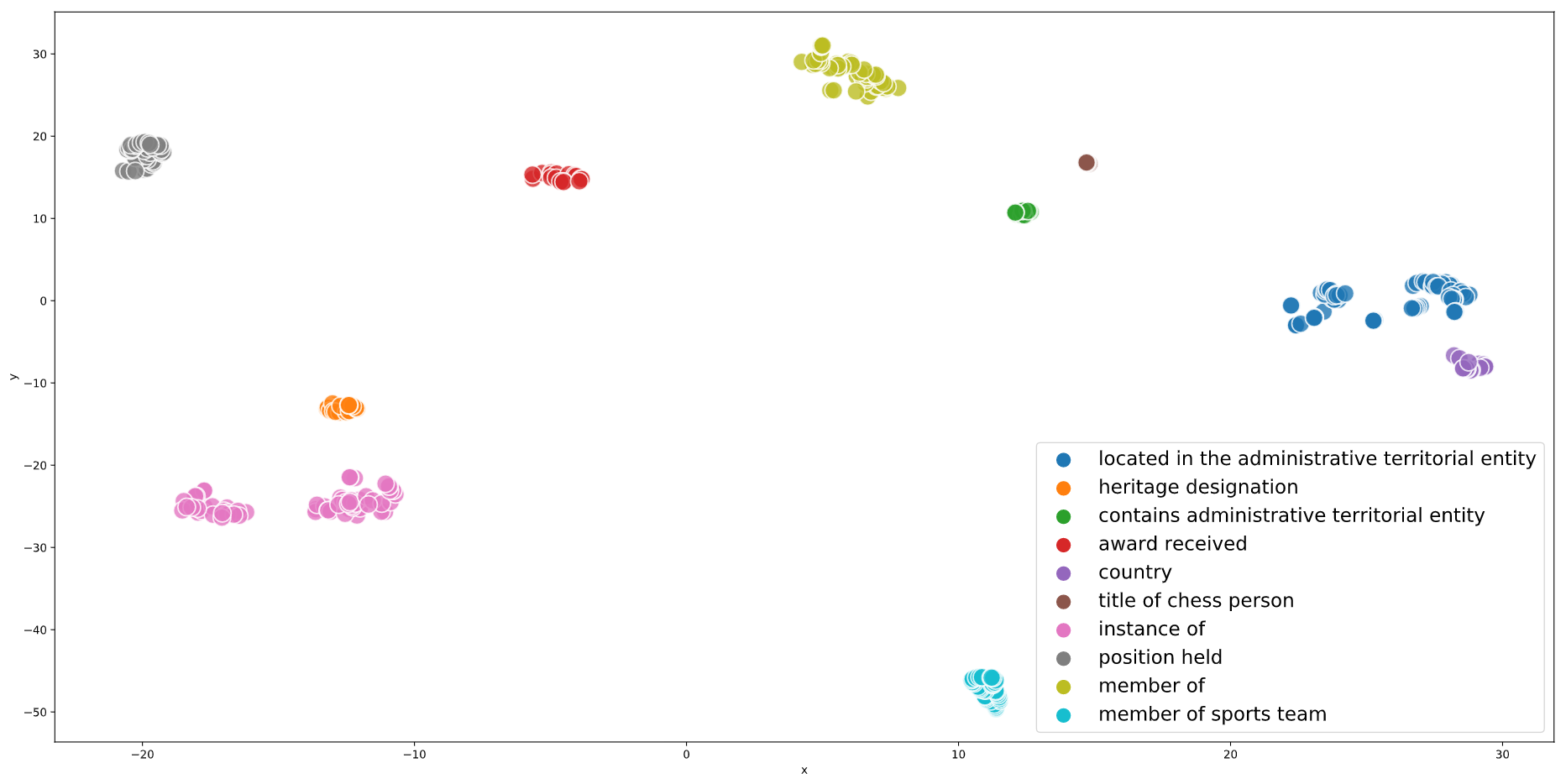
Figure 1: Two-dimensional t-SNE projection of the embedding learned by the model. For legibility, only the ten most common predicates are plotted.

Additionally, we note that predicates with many points seem to form lines or circles in the reduced dimensionality plot. To investigate this, we took the same t-SNE embeddings and created a plot containing just the predicate member of sports team (P54). This plot is displayed in Figure 2(b). It shows that the model has successfully learned a somewhat smooth temporal evolution of the embedding: each step in time moves the embedding in a similar direction, and the different points in time are well separated.

To evaluate how much of this is due to SpliMe, we also plot a baseline dataset obtained by applying random splits, as described in Section 4.2, for a predicate that had an approximately equal number of splits. The original could not be used as none of our random baseline models had the required number of splits for that predicate. Figure 2(a) shows that here the temporal evolution of the embedding is completely erratic. This implies that SpliMe includes temporal scopes in an intelligent manner.

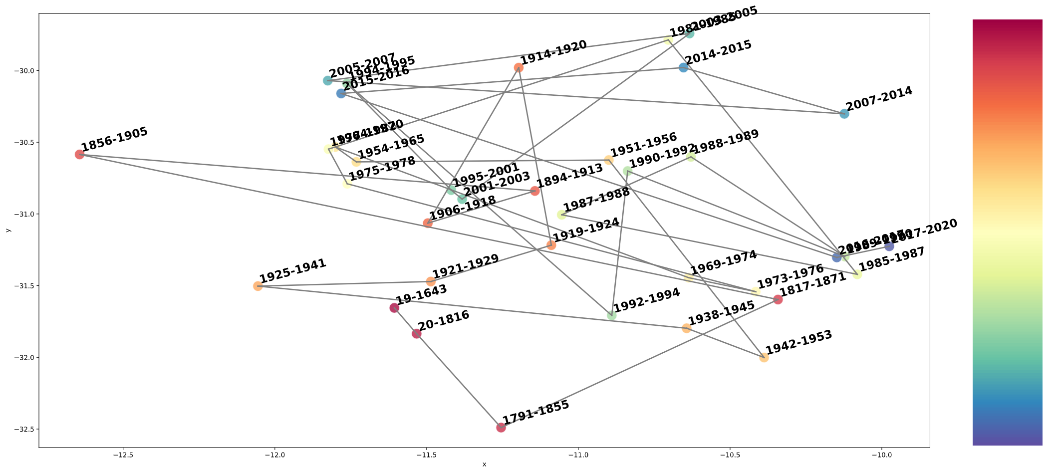
(a) t-SNE plot of a dataset created by applying splits randomly. Only the residence (P551) predicate is drawn.

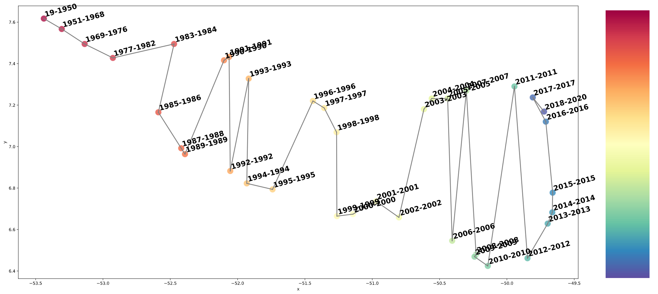
(b) t-SNE plot of a dataset created using the SpliMe merge method. Only the member of sports team (P54) predicate is drawn.

Figure 2: Two t-SNE projections. The colors are based on the end-time of the predicate, ranging from red (long ago) to blue (recent). The lines between the points illustrate how the embedding moves through the vector space, and the labels denote the time period during which the predicate is valid.

Appendix 0.D Change Point Detection in SpliMe

In this section we give a more detailed explanation of CPD and how it relates to SpliMe. Specifically, we will discuss the cost function and kernel method as used by SpliMe during change point detection. For a complete overview of kernel functions in CPD we also refer to [8].

Broadly speaking, CPD algorithms can be divided into two categories: online and offline. Online CPD analyses a time series of unknown (possibly infinite) length. The decision on whether a change point has occurred is made every time a new data point arrives. In contrast, offline CPD considers the entire data set at once and can thus look back in time to see when a change occurred. For SpliMe, the length of the time series is already known. Therefore, we are only interested in offline CPD. A survey of offline CPD algorithms can be found in [25].

As noted earlier, we employ the typology defined in [25]. That is, CPD is a model selection problem which consists of selecting the ”best” possible segmentation of a time series. A CPD algorithm has three components a cost function, a search method and a constraint (on the number of change points). The cost function is a measure of homogeneity, i.e., how similar data points in a given segment are. The search method concerns locating possible segment boundaries, i.e., it locates parts of the signal that should be grouped together. The best possible segmentation is the one that minimizes the associated cost function.

Let $S=\{x_{1},x_{2},\dots,x_{l}\}$ denote a time series, and $L=\{k_{1},\ldots,k_{K}\}$, $0\leq K\leq l\in\mathbb{N}^{+}$ denote a possible segmentation of that time series. As explained in Section 3.2, SpliMe creates a time series for every predicate in the graph. For each such time series $S_{r}\ r\in\mathcal{P}$, its entries $x_{i},\ldots,x_{l}$ are vectors containing the proximity scores between pairs of nodes in the graph. These scores are calculated using only edges consisting of the predicate $r$ which exist at the given timestamp.

Because these vectors signify proximity scores, the data does not necessarily occupy a euclidean space. As a result, we cannot use tradition distance metrics such as the $\ell_{1}$ and $\ell_{2}$ norms to calculate the distance between two samples. Instead, a kernel function is used instead to map the data to a different space in which a comparison can be made. To do this, SpliMe uses the well known radial basis function kernel, defined as

$$\mathit{rbf}(x_{1},x_{2})=\exp(-\gamma||x_{1}-x_{2}||^{2})$$

Here, $x_{1}$ and $x_{2}$ are the two samples from $S_{r}$ being evaluated. $||\cdot||^{2}$ is the $\ell_{2}$-norm and $\gamma>0$ is the bandwidth parameter determined according to the median heuristic.

As a cost function SpliMe uses kernelized mean change. Like the well known sum of squares metric, kernelized mean change calculates how far each sample lies from the (empirical) mean and sums the result. However, each sample is first translated with the $rbf$. Formally, the cost function for a subsection of the signal can be written as

$$c(S_{a,b})=\sum_{a\leq i<b}=||\mathit{rbf}(S_{i})-\overline{\mu}_{a,b}||^{2}$$

where $\overline{\mu}_{a,b}$ denotes the empirical mean of the subsection in the transformed space. The total cost $cost(\cdot)$ for a segmentation $L$ then is the summation of the costs of each segment, i.e.,

$$cost(L)=\sum_{i=1}^{K-1}c(S_{L_{i},L_{i+1}})$$

Appendix 0.E Extended Related Work

In this section we will provide an overview of several related static knowledge graph embedding works. A thorough list of static KG embedding models can be found in [12, 21]. Firstly, as one of the earliest link prediction methods, Liben-Nowell et al. [19] apply network proximity measures to the problem of link prediction in homogenous graphs (e.g. social networks). Explained in detail in Section 2, network proximity measures calculate the proximity between a pair of nodes in a graph based on the graphs structure. Specifically, their measures calculate proximity scores for (a selection of) pairs of nodes in a graph. The pairs with the highest scores are the most similar and are intuitively the most likely to form a new link.

0.E.1 Representation Learning

Current state-of-the-art KG embedding methods perform representation learning. I.e., they learn a vector representation of the entities and predicates making up a KG. These vectors represent the latent features of entities and relationships: the underlying parameters that determine their interactions.

Roughly speaking, KG embedding approaches using latent features can be defined in two groups, translational approaches and tensor-factorization approaches. Models of the first type apply meaning to latent representation: entities that are similar must be close together according to some distance measure. Models of the second type do not apply any meaning to the embedding themselves, but capture the underlying interactions directly. We will now give an overview of several important KG embedding models, including an overview of some temporal KG embedding models.

0.E.1.1 Translational Models

One of the most well known embedding models is TransE [4]. It is based on the intuition that summing the subject and predicate embedding vectors should result in a vector approximately equal to the object embedding vector. Scores are assigned based on the $\ell_{1}$ or $\ell_{2}$ norms between the expected and actual object embedding.

TransH [26] further increases the expressiveness of TransE by enabling each entity to have a unique representation for each predicate. This is achieved by modelling each predicate with two vectors. The first defines a hyperplane, the second defines the translation on that hyperplane. When calculating distance, the entity vectors are first projected on the predicate-specific hyperplane using the dot product.

0.E.1.2 Factorization models

One of the oldest factorization models is Canonical Polyadic (CP) decomposition. CP was long thought to be unsuitable for KGE because it learns separate representations for subject and object occurrences of an entity. However, [15] propose a simple enhancement to CP that addresses this independence, called SimplE. Specifically, they learn an additional inverse embedding for each predicate. The score of a triple is then calculated by taking the average between its normal score and its inverse score.

ComplEx [24] observe that while the representation of an entity should be equal regardless of whether it occurs as a subject or as an object in a triple, its behavior should not be. Noting that the definition of the dot product on complex numbers is not symmetric, they suggest combining complex vectors with a dot product based scoring function. Now, the representation of an entity is the same, but its behavior depends on whether it is used as object or subject.

RotatE [22] models entities and predicates with complex vectors, and then views relations as rotations from the subject to the object entity in the complex space. The authors go on to define several relationship patterns and prove that RotatE can, unlike its competitors, model all of these.

References

- [1] Adamic, L.A., Adar, E.: Friends and neighbors on the web. Soc. Networks 25(3), 211–230 (2003)
- [2] Aminikhanghahi, S., Cook, D.J.: A survey of methods for time series change point detection. Knowl. Inf. Syst. 51(2), 339–367 (2017)
- [3] Bastos, A., Nadgeri, A., Singh, K., Mulang, I.O., Shekarpour, S., Hoffart, J.: RECON: relation extraction using knowledge graph context in a graph neural network. CoRR abs/2009.08694 (2020)
- [4] Bordes, A., Usunier, N., García-Durán, A., Weston, J., Yakhnenko, O.: Translating embeddings for modeling multi-relational data. In: 27th Annual Conference on Neural Information Processing Systems 2013. pp. 2787–2795 (2013)
- [5] Costabello, L., Pai, S., Van, C.L., McGrath, R., McCarthy, N., Tabacof, P.: AmpliGraph: a Library for Representation Learning on Knowledge Graphs (Mar 2019)
- [6] Dasgupta, S.S., Ray, S.N., Talukdar, P.P.: Hyte: Hyperplane-based temporally aware knowledge graph embedding. In: Proceedings of the 2018 Conference on Empirical Methods in Natural Language Processing. pp. 2001–2011. ACL (2018)
- [7] García-Durán, A., Dumancic, S., Niepert, M.: Learning sequence encoders for temporal knowledge graph completion. In: Proceedings of the 2018 Conference on Empirical Methods in Natural Language Processing. pp. 4816–4821. ACL (2018)
- [8] Garreau, D.: Change-point detection and kernel methods. Theses, Université Paris sciences et lettres (Oct 2017)
- [9] Goel, R., Kazemi, S.M., Brubaker, M., Poupart, P.: Diachronic embedding for temporal knowledge graph completion. In: Proeceedings of the Thirty-Fourth Conference on Artificial Intelligence, AAAI. pp. 3988–3995. AAAI Press (2020)
- [10] Guo, Q., Zhuang, F., Qin, C., Zhu, H., Xie, X., Xiong, H., He, Q.: A survey on knowledge graph-based recommender systems. CoRR abs/2003.00911 (2020)
- [11] Huang, X., Zhang, J., Li, D., Li, P.: Knowledge graph embedding based question answering. In: Proceedings of the Twelfth ACM International Conference on Web Search and Data Mining, WSDM. pp. 105–113. ACM (2019)
- [12] Ji, S., Pan, S., Cambria, E., Marttinen, P., Yu, P.S.: A survey on knowledge graphs: Representation, acquisition and applications. CoRR abs/2002.00388 (2020)
- [13] Jiang, T., Liu, T., Ge, T., Sha, L., Li, S., Chang, B., Sui, Z.: Encoding temporal information for time-aware link prediction. In: Proceedings of the 2016 Conference on Empirical Methods in Natural Language Processing, EMNLP, 2016. pp. 2350–2354. ACL (2016)
- [14] Jin, W., Qu, M., Jin, X., Ren, X.: Recurrent event network: Autoregressive structure inferenceover temporal knowledge graphs. In: Proceedings of the 2020 Conference on Empirical Methods in Natural Language Processing, EMNLP. pp. 6669–6683. ACL (2020)
- [15] Kazemi, S.M., Poole, D.: Simple embedding for link prediction in knowledge graphs. In: Advances in Neural Information Processing Systems 31, NeurIPS 2018. pp. 4289–4300 (2018)
- [16] Kingma, D.P., Ba, J.: Adam: A method for stochastic optimization. In: 3rd International Conference on Learning Representations, ICLR 2015 (2015)
- [17] Lacroix, T., Obozinski, G., Usunier, N.: Tensor decompositions for temporal knowledge base completion. In: 8th International Conference on Learning Representations, ICLR 2020. OpenReview.net (2020)
- [18] Leblay, J., Chekol, M.W.: Deriving validity time in knowledge graph. In: Companion of the The Web Conference 2018 on The Web Conference 2018, WWW. pp. 1771–1776. ACM (2018)
- [19] Liben-Nowell, D., Kleinberg, J.M.: The link-prediction problem for social networks. J. Assoc. Inf. Sci. Technol. 58(7), 1019–1031 (2007)
- [20] van der Maaten, L., Hinton, G.: Visualizing data using t-sne. Journal of Machine Learning Research 9(86), 2579–2605 (2008)
- [21] Nickel, M., Murphy, K., Tresp, V., Gabrilovich, E.: A review of relational machine learning for knowledge graphs. Proc. IEEE 104(1), 11–33 (2016)
- [22] Sun, Z., Deng, Z., Nie, J., Tang, J.: Rotate: Knowledge graph embedding by relational rotation in complex space. In: 7th International Conference on Learning Representations, ICLR 2019. OpenReview.net (2019)
- [23] Tang, X., Yuan, R., Li, Q., Wang, T., Yang, H., Cai, Y., Song, H.: Timespan-aware dynamic knowledge graph embedding by incorporating temporal evolution. IEEE Access 8, 6849–6860 (2020)
- [24] Trouillon, T., Welbl, J., Riedel, S., Gaussier, É., Bouchard, G.: Complex embeddings for simple link prediction. In: Proceedings of the 33nd International Conference on Machine Learning, ICML 2016. JMLR Workshop and Conference Proceedings, vol. 48, pp. 2071–2080. JMLR.org (2016)
- [25] Truong, C., Oudre, L., Vayatis, N.: Selective review of offline change point detection methods. Signal Process. 167 (2020)
- [26] Wang, Z., Zhang, J., Feng, J., Chen, Z.: Knowledge graph embedding by translating on hyperplanes. In: Proceedings of the Twenty-Eighth Conference on Artificial Intelligence, AAAI 2014. pp. 1112–1119. AAAI Press (2014)
- [27] Xu, C., Nayyeri, M., Alkhoury, F., Lehmann, J., Yazdi, H.S.: Temporal knowledge graph embedding model based on additive time series decomposition. CoRR abs/1911.07893 (2019)