Joint Majorization-Minimization for Nonnegative Matrix Factorization with the $\beta$-divergence

Abstract

This article proposes new multiplicative updates for nonnegative matrix factorization (NMF) with the $\beta$-divergence objective function. Our new updates are derived from a joint majorization-minimization (MM) scheme, in which an auxiliary function (a tight upper bound of the objective function) is built for the two factors jointly and minimized at each iteration. This is in contrast with the classic approach in which a majorizer is derived for each factor separately. Like that classic approach, our joint MM algorithm also results in multiplicative updates that are simple to implement. They however yield a significant drop of computation time (for equally good solutions), in particular for some $\beta$-divergences of important applicative interest, such as the quadratic loss and the Kullback-Leibler or Itakura-Saito divergences. We report experimental results using diverse datasets: face images, an audio spectrogram, hyperspectral data and song play counts. Depending on the value of $\beta$ and on the dataset, our joint MM approach can yield CPU time reductions from about $13\%$ to $86\%$ in comparison to the classic alternating scheme.

This work is supported by the European Research Council (ERC FACTORY-CoG-6681839), the French Agence Nationale de la Recherche (ANITI, ANR-19-P3IA-0004) and the National Research Foundation, Prime Minister’s Office, Singapore under its Campus for Research Excellence and Technological Enterprise (CREATE) programme.

1 Introduction

Nonnegative matrix factorization (NMF) aims at factorizing a matrix with nonnegative entries into the product of two nonnegative matrices. It has found many applications in various domains which include feature extraction in image processing and text mining [1], audio source separation [2], blind unmixing in hyperspectral imaging [3, 4], and user recommendation [5]. See [6, 7, 8] for overview papers and books about NMF.

Each application gives different interpretations to the factor matrices but the first factor is often considered as a dictionary of recurring patterns while the second one describes how the data samples are expanded onto the dictionary (activation matrix). The nonnegativity constraint only allows additive combination of the dictionary elements, yielding meaningful additive and sparse representations of the data.

Computing an NMF generally consists in minimizing a well-chosen objective function under nonnegativity constraints. A popular choice of objective function is the $\beta$-divergence, which is a continuous family of measures of fit parameterized by a single parameter $\beta$ that encompasses the Kullback-Leibler (KL) or Itakura-Saito (IS) divergences as well as the common squared Euclidean distance [9]. In the latter cases, the $\beta$-divergence is a log-likelihood in disguise for Poisson, multiplicative Gamma and additive Gaussian noise models, respectively.

The classic approach to NMF, and to NMF with the $\beta$-divergence in particular, consists in optimizing the two factors alternately, i.e., using two-block coordinate descent. Each of the two factors is then updated using Majorization-Minimization (MM), as described in [10, 11, 12, 13, 14]: given one of the factors, a tight upper bound of the objective function is constructed and minimized with respect to (w.r.t) the other factor. This results in multiplicative updates that are simple to implement (with no hyperparameter to tune), have linear complexity per iteration, and that automatically preserve nonnegativity given positive initializations. By construction, MM ensures monotonicity of the objective function (non-increasing values), see [15, 16] for tutorials about MM.

Thanks to its simplicity, the block-descent approach is dominant in matrix factorization and dictionary learning (using sometimes other block partitions such as columns or rows [6, 8]) and very few works have addressed joint (“all-at-once”) optimization of the factors, though the latter approach may be more efficient. A notable exception in dictionary learning (real-valued factors, sparse activations, quadratic loss) is [17]. In this work, the author employs an elegant non-convex proximal splitting strategy and shows that the joint approach is significantly faster than alternating methods without altering the quality of the obtained solution. In a similar spirit to [17], [18] leverages the theoretical framework of [19] to address matrix factorization (including NMF) with non-alternating updates. Their work relies on the generalization of Lipschitz-continuity of the gradient (which does not hold jointly for both factors) to adaptive smoothness [19]. Yet, their results only apply to the quadratic loss and Newton-like acceleration is crucial to obtain competitive results. Using tools from dynamical systems, the authors in [20] have derived a novel form of multiplicative updates which can run concurrently for each factor matrix at a given iteration. They have the additional benefit of ensuring the convergence to a local minimum instead of a mere critical point. However, their results are again limited to the quadratic loss. This also applies to [21] where a Levenberg-Marquardt joint optimization method is described for NMF with the quadratic loss. In [22], the authors propose a joint second-order Newton-like algorithm for nonnegative canonical tensor decomposition with the $\beta$-divergence, which takes NMF as a special case. Their approach relies on approximations of the Hessian matrix, sometimes based on heuristics, and fails to provide an algorithm that universally works for every value of $\beta$.

Inspired by these works, we propose a joint MM approach to $\beta$-NMF and compare it to the classic block MM strategy. Our joint MM relies on a tight majorization of the objective function with respect to all its variables instead of using blocks of fixed variables. Iterative minimization of this joint upper bound results in new multiplicative updates that are simple but potentially more efficient variants of the classical multiplicative updates. This is particularly true when considering the quadratic loss and the KL or IS divergences for which further simplifications occur. We show in these cases that our update rules decrease the computation cost per iteration. It turns out that our joint upper bound coincides with the one derived in [23]. The latter is however employed for a different purpose, namely the convergence analysis of classic block MM for NMF, and not to design a new algorithm like we do (more details will be given in Section 3.3).

Our methodological results are supported by extensive simulations using datasets with different sizes arising from various applications in which NMF had a significant impact (face images, audio spectrogram, hyperspectral images, song play-counts). In most scenarii, the proposed joint MM approach leads to a reduction of the computing time ranging from $13\%$ to $86\%$ without incurring any loss in the precision of the approximation.

The article is organized as follows: Section 2 states the NMF optimization problem and summarizes the classic block MM approach. Section 3 first presents our proposed joint MM method for NMF and derives the new multiplicative updates. It then compares the joint and the block MM methods in term of computational complexity, and discusses the benefit of the joint approach. Comparative numerical simulations are presented in Section 4 and validate the efficiency of our approach. Finally, Section 5 draws conclusions.

Notation

$\mathbb{R}_{+}$ is the set of nonnegative real numbers, and $\llbracket 1,N\rrbracket$ is the set of integers from $1$ to $N$. Bold upper case letters denote matrices, bold lower case letters denote vectors, and lower case letters denote scalars. The notation ${[\mathbf{M}]}_{ij}$ and $m_{ij}$ both stand for the element of $\mathbf{M}$ located at the $i^{\text{th}}$ row and the $j^{\text{th}}$ column. For a matrix $\mathbf{M}$, the notation $\mathbf{M}\geq 0$ denotes entry-wise nonnegativity.

2 Preliminaries

2.1 Nonnegative matrix factorization

We aim at factorizing a $F\times N$ nonnegative matrix $\mathbf{V}$ into the product $\mathbf{W}\mathbf{H}$ of two nonnegative factor matrices of sizes $F\times K$ and $K\times N$, respectively. The rank value $K$ is often chosen such that $FK+KN\ll FN$, leading to a low-rank approximation of $\mathbf{V}$. Given a desired value for the rank $K$, the factor matrices are obtained by solving the following optimization problem

$$\min_{\mathbf{W},\mathbf{H}\geq 0}D_{\beta}(\mathbf{V}\mid\mathbf{W}\mathbf{H})\,,$$ (1)

where $D_{\beta}$ is a separable objective function defined by

$$D_{\beta}(\mathbf{V}\mid\mathbf{W}\mathbf{H})=\sum_{f=1}^{F}\sum_{n=1}^{N}d_{\beta}(v_{fn}\mid{[\mathbf{W}\mathbf{H}]}_{fn})\,.$$ (2)

Our measure of fit $d_{\beta}$ is the $\beta$-divergence [9] given by

$$d_{\beta}(x\mid y)=\begin{cases*}x\log\frac{x}{y}-x+y&if $\beta=1$\\ \frac{x}{y}-\log\frac{x}{y}-1&if $\beta=0$\\ \frac{x^{\beta}}{\beta(\beta-1)}+\frac{y^{\beta}}{\beta}-\frac{xy^{\beta-1}}{\beta-1}&otherwise.\end{cases*}$$ (3)

The value of $\beta$ is chosen according to the application context and the noise assumptions on $\mathbf{V}$ [13]. The IS divergence, KL divergence and quadratic loss are obtained for $\beta=0,1,2$, respectively.

2.2 Classic multiplicative updates

The classic method to solve Problem (1) consists in a two-block coordinate descent approach where each block is handled with MM. Namely, it alternately minimizes $(\mathbf{W},\mathbf{H})\mapsto D_{\beta}(\mathbf{V}|\mathbf{W}\mathbf{H})$ in $\mathbf{W}$ and in $\mathbf{H}$ using MM. The MM method is a two-step iterative optimization scheme [15, 16]. At each iteration, the first step consists in building a local auxiliary function $G$ that is minimized in the second step. The auxiliary function has to be a tight majorizer of the original objective function $\phi:\mathbb{E}\mapsto\mathbb{R}$ at the current iterate $\tilde{\mathbf{x}}$, where $\mathbb{E}$ is the domain of $G$ and $\phi$. More precisely, it has to satisfy the following two properties:

$$\left(\forall\mathbf{x}\in\mathbb{E}\right)\quad G(\mathbf{x}\mid\tilde{\mathbf{x}}) \geq\phi(\mathbf{x})$$

$$G(\tilde{\mathbf{x}}\mid\tilde{\mathbf{x}}) =\phi(\tilde{\mathbf{x}})\,.$$

These properties ensure that any iterate $\mathbf{x}$ that decreases the value of $G$ also decreases the value of $\phi$. Indeed, for a given $\tilde{\mathbf{x}}$, if we find $\mathbf{x}$ such that $G(\mathbf{x}|\tilde{\mathbf{x}})\leq G(\tilde{\mathbf{x}}|\tilde{\mathbf{x}})$, then the tight majorization properties induce the following descent lemma

$$\phi(\mathbf{x})\leq G(\mathbf{x}\mid\tilde{\mathbf{x}})\leq G(\tilde{\mathbf{x}}\mid\tilde{\mathbf{x}})=\phi(\tilde{\mathbf{x}})\,.$$ (4)

Note that even if $G$ is not minimized but only decreased in value, the descent property still holds.

The previous MM scheme can be applied alternately to the minimization of the two functions $\mathbf{W}\mapsto D_{\beta}(\mathbf{V}|\mathbf{W}\mathbf{H})$ and $\mathbf{H}\mapsto D_{\beta}(\mathbf{V}|\mathbf{W}\mathbf{H})$. These two functions are the sum of concave, convex, and constant terms. A convex auxiliary function can then be easily derived by using Jensen’s inequality for the convex term and the tangent inequality for the concave term, see [13] and the next section. This yields the following multiplicative updates

$$\mathbf{W} \;\longleftarrow\;\mathbf{W}.{\left(\frac{\left({(\mathbf{W}\mathbf{H})}^{.(\beta-2)}.\mathbf{V}\right)\mathbf{H}^{\top}}{\left({(\mathbf{W}\mathbf{H})}^{.(\beta-1)}\right)\mathbf{H}^{\top}}\right)}^{.\gamma(\beta)}$$ (5)

$$\mathbf{H} \;\longleftarrow\;\mathbf{H}.{\left(\frac{\mathbf{W}^{\top}\left({(\mathbf{W}\mathbf{H})}^{.(\beta-2)}.\mathbf{V}\right)}{\mathbf{W}^{\top}\left({(\mathbf{W}\mathbf{H})}^{.(\beta-1)}\right)}\right)}^{.\gamma(\beta)}\,,$$

where . and $/$ are the entry-wise multiplication and division, respectively, and $\gamma(\beta)$ is a scalar defined as

$$\gamma(\beta)=\begin{cases*}\frac{1}{2-\beta}&if $\beta\in]-\infty,1[$\\ 1&if $\beta\in[1,2]$\\ \frac{1}{\beta-1}&if $\beta\in]2,+\infty[$\end{cases*}\,.$$ (6)

Note that by construction, the matrices $\mathbf{W}$ and $\mathbf{H}$ resulting from the update (5) contain only positive coefficients if the input matrices $\mathbf{V}$, $\mathbf{W}$, and $\mathbf{H}$ are all positive. The nonnegativity of the iterates is thus preserved by the multiplicative structure of the updates given positive initializations.

Note that strict MM dictates that the individual updates of $\mathbf{W}$ and $\mathbf{H}$ given in (5) shall be applied several times to fully minimize the partial functions $\mathbf{W}\mapsto D_{\beta}(\mathbf{V}|\mathbf{W}\mathbf{H})$ and $\mathbf{H}\mapsto D_{\beta}(\mathbf{V}|\mathbf{W}\mathbf{H})$. This leads to Algorithm 1, that we refer to as Block MM (BMM). Note that in common NMF practice, only one sub-iteration is used ($L_{W}=L_{H}=1$), which still results in a descent algorithm thanks to the descent lemma (4).

0:  Nonnegative matrix $\mathbf{V}$ and initialization $(\mathbf{W}_{\text{init}},\mathbf{H}_{\text{init}})$

0:  Nonnegative matrices $\mathbf{W}$ and $\mathbf{H}$ such that $\mathbf{V}\approx\mathbf{W}\mathbf{H}$

1:  Initialize $i$ to $1$

2:  Initialize $(\bm{\check{\mathbf{W}}}_{i},\bm{\check{\mathbf{H}}}_{i})$ to $(\mathbf{W}_{\text{init}},\mathbf{H}_{\text{init}})$

3:  repeat

4:     Initialize $\mathbf{W}_{1}$ to $\bm{\check{\mathbf{W}}}_{i}$

5:     for $l=1\dots L_{W}$ do

6:        Update $\mathbf{W}$ using (5)

$$\mathbf{W}_{l+1}\longleftarrow\mathbf{W}_{l}.{\left(\frac{\left({(\mathbf{W}_{l}\bm{\check{\mathbf{H}}}_{i})}^{.(\beta-2)}.\mathbf{V}\right)\bm{\check{\mathbf{H}}}_{i}^{\top}}{\left({(\mathbf{W}_{l}\bm{\check{\mathbf{H}}}_{i})}^{.(\beta-1)}\right)\bm{\check{\mathbf{H}}}_{i}^{\top}}\right)}^{.\gamma(\beta)}$$

7:     end for

8:     $\bm{\check{\mathbf{W}}}_{i+1}\leftarrow\mathbf{W}_{L_{W}+1}$

9:     Initialize $\mathbf{H}_{1}$ to $\bm{\check{\mathbf{H}}}_{i}$

10:     for $l=1\dots L_{H}$ do

11:        Update $\mathbf{H}$ using (5)

$$\mathbf{H}_{l+1}\longleftarrow\mathbf{H}_{l}.{\left(\frac{\bm{\check{\mathbf{W}}}_{i+1}^{\top}\left({(\bm{\check{\mathbf{W}}}_{i+1}\mathbf{H}_{l})}^{.(\beta-2)}.\mathbf{V}\right)}{\bm{\check{\mathbf{W}}}_{i+1}^{\top}\left({(\bm{\check{\mathbf{W}}}_{i+1}\mathbf{H}_{l})}^{.(\beta-1)}\right)}\right)}^{.\gamma(\beta)}$$

12:     end for

13:     $\bm{\check{\mathbf{H}}}_{i+1}\leftarrow\mathbf{H}_{L_{H}+1}$

14:     Increment $i$

15:  until Convergence

16:  return  $(\bm{\check{\mathbf{W}}}_{i},\bm{\check{\mathbf{H}}}_{i})$

Algorithm 1 BMM 

3 Joint Majorization-Minimization

In contrast with the classic alternating scheme presented in Section 2.2, we develop in this section a joint MM (JMM) approach for solving Problem (1).

3.1 Construction of the auxiliary function

In order to apply the MM scheme, we start by looking for a suitable auxiliary function $G:\mathbb{R}_{+}^{F\times K}\times\mathbb{R}_{+}^{K\times N}\rightarrow\mathbb{R}_{+}$ for the function $(\mathbf{W},\mathbf{H})\mapsto D_{\beta}(\mathbf{V}|\mathbf{W}\mathbf{H})$. We observe in (2) that $D_{\beta}$ is a sum of $FN$ $\beta$-divergences between scalars. Our approach is to construct an auxiliary function for each summand. Following [13], the $\beta$-divergence $d_{\beta}$, taken as a function of its second argument, can be decomposed into the sum of a convex term $\smash{\overset{\scriptscriptstyle\smile}{d}}_{\beta}$, a concave term $\smash{\overset{\scriptscriptstyle\frown}{d}}_{\beta}$, and a constant term $\bar{d}_{\beta}$. The definitions of these three terms for the different values of $\beta$ are given in Table 1.

Table 1: Decomposition of $d_{\beta}$ for the different values of $\beta$.

$\beta$	$\smash{\overset{\scriptscriptstyle\smile}{d}}_{\beta}(v_{fn}\mid{[\mathbf{W}\mathbf{H}]}_{fn})$	$\smash{\overset{\scriptscriptstyle\frown}{d}}_{\beta}(v_{fn}\mid{[\mathbf{W}\mathbf{H}]}_{fn})$	$\bar{d}_{\beta}(v_{fn})$
$]-\infty,1[\setminus\{0\}$	$\frac{-v_{fn}}{\beta-1}{[\mathbf{W}\mathbf{H}]}_{fn}^{\beta-1}$	$\frac{{[\mathbf{W}\mathbf{H}]}_{fn}^{\beta}}{\beta}$	$\frac{v_{fn}^{\beta}}{\beta(\beta-1)}$
$0$	$\frac{v_{fn}}{{[\mathbf{W}\mathbf{H}]}_{fn}}$	$\log{[\mathbf{W}\mathbf{H}]}_{fn}$	$-(\log v_{fn}+1)$
$[1,2]$	$d_{\beta}(v_{fn}\mid{[\mathbf{W}\mathbf{H}]}_{fn})$	$0$	$0$
$]2,+\infty[$	$\frac{{[\mathbf{W}\mathbf{H}]}_{fn}^{\beta}}{\beta}$	$\frac{-v_{fn}}{\beta-1}{[\mathbf{W}\mathbf{H}]}_{fn}^{\beta-1}$	$\frac{v_{fn}^{\beta}}{\beta(\beta-1)}$

Next, we majorize the convex and concave terms of $d_{\beta}$ separately. The methodology follows [13], except that none of the two factors $\mathbf{W}$ or $\mathbf{H}$ is treated as a fixed variable. The convex term $\smash{\overset{\scriptscriptstyle\smile}{d}}_{\beta}$ is majorized using Jensen’s inequality

$$\smash{\overset{\scriptscriptstyle\smile}{d}}_{\beta}(v_{fn}\mid{[\mathbf{W}\mathbf{H}]}_{fn}) =\smash{\overset{\scriptscriptstyle\smile}{d}}_{\beta}\left(v_{fn}\;\middle|\;\sum_{k=1}^{K}w_{fk}h_{kn}\right)$$

$$=\smash{\overset{\scriptscriptstyle\smile}{d}}_{\beta}\left(v_{fn}\;\middle|\;\sum_{k=1}^{K}\tilde{\lambda}_{fnk}\frac{w_{fk}h_{kn}}{\tilde{\lambda}_{fnk}}\right)$$

$$\leq\sum_{k=1}^{K}\tilde{\lambda}_{fnk}\smash{\overset{\scriptscriptstyle\smile}{d}}_{\beta}\left(v_{fn}\;\middle|\;\frac{w_{fk}h_{kn}}{\tilde{\lambda}_{fnk}}\right)$$ (7)

$$\stackrel{{\scriptstyle\mbox{\footnotesize def}}}{{=}}\smash{\overset{\scriptscriptstyle\smile}{G}}_{fn}(\mathbf{W},\mathbf{H}\mid\bm{\tilde{\mathbf{W}}},\bm{\tilde{\mathbf{H}}})\,,$$

where the coefficient $\tilde{\lambda}_{fnk}$ is defined as $\tilde{\lambda}_{fnk}=\frac{\tilde{w}_{fk}\tilde{h}_{kn}}{\tilde{v}_{fn}}$ and we denote $\bm{\tilde{\mathbf{V}}}=\bm{\tilde{\mathbf{W}}}\bm{\tilde{\mathbf{H}}}$ with coefficients $\tilde{v}_{fn}$. The concave term $\smash{\overset{\scriptscriptstyle\frown}{d}}_{\beta}$ is majorized using the tangent inequality

$$\smash{\overset{\scriptscriptstyle\frown}{d}}_{\beta} (v_{fn}\mid{[\mathbf{W}\mathbf{H}]}_{fn})$$

$$\leq\smash{\overset{\scriptscriptstyle\frown}{d}}_{\beta}(v_{fn}\mid\tilde{v}_{fn})+\smash{\overset{\scriptscriptstyle\frown}{d^{\prime}}}_{\beta}(v_{fn}\mid\tilde{v}_{fn})\left({[\mathbf{W}\mathbf{H}]}_{fn}-\tilde{v}_{fn}\right)$$

$$\stackrel{{\scriptstyle\mbox{\footnotesize def}}}{{=}}\smash{\overset{\scriptscriptstyle\frown}{G}}_{fn}(\mathbf{W},\mathbf{H}|\bm{\tilde{\mathbf{W}}},\bm{\tilde{\mathbf{H}}})\,.$$

Finally the overall auxiliary function $G$ is given by

$$G=\sum_{f=1}^{F}\sum_{n=1}^{N}\left[\smash{\overset{\scriptscriptstyle\smile}{G}}_{fn}+\smash{\overset{\scriptscriptstyle\frown}{G}}_{fn}+\bar{d}_{\beta}\right]\,.$$ (8)

By construction, it satisfies the tight majorization properties

$$G(\mathbf{W},\mathbf{H}\mid\bm{\tilde{\mathbf{W}}},\bm{\tilde{\mathbf{H}}})\geq D_{\beta}(\mathbf{V}\mid\bm{\tilde{\mathbf{W}}}\bm{\tilde{\mathbf{H}}})$$

$$G(\bm{\tilde{\mathbf{W}}},\bm{\tilde{\mathbf{H}}}\mid\bm{\tilde{\mathbf{W}}},\bm{\tilde{\mathbf{H}}})=D_{\beta}(\mathbf{V}\mid\bm{\tilde{\mathbf{W}}}\bm{\tilde{\mathbf{H}}})\,,$$

which ensure the descent property in (4). The expression of $G$ coincides with the joint auxiliary function derived in [23, Table 2 in Section 4 and Appendix A] for a different purpose (see Section 3.3.4).

We stress out that the auxiliary function $G$ is a tight joint majorization of $D_{\beta}$. This is in contrast with the BMM approach of Section 2.2 where two separate auxiliary functions $G_{\mathbf{W}}$ and $G_{\mathbf{H}}$ are built for $\mathbf{W}\mapsto D_{\beta}(\mathbf{V}|\mathbf{W}\mathbf{H})$ and $\mathbf{H}\mapsto D_{\beta}(\mathbf{V}|\mathbf{W}\mathbf{H})$, respectively. A central difference in our JMM approach is the definition of the coefficients $\{\tilde{\lambda}_{fnk}\}$ which depend on both current iterates $\bm{\tilde{\mathbf{W}}}$ and $\bm{\tilde{\mathbf{H}}}$ and do not lead to a simplification of the term $w_{fk}h_{kn}/\tilde{\lambda}_{fnk}$ in (7). This is in contrast with BMM, where, say, $\mathbf{W}$ would be treated as a fixed variable and the term $w_{fk}h_{kn}/\tilde{\lambda}_{fnk}$ simplifies to $\tilde{v}_{fn}h_{kn}/\tilde{h}_{kn}$, allowing for closed-form minimization of $G$. Furthermore, the auxiliary function $G$ is not jointly convex, due to the bilinear terms $w_{fk}h_{kn}$. It is however bi-convex, i.e., convex w.r.t $\mathbf{W}$ (resp., $\mathbf{H}$) given $\mathbf{H}$ (resp., $\mathbf{W}$).

3.2 Minimization step

The auxiliary function $G$ does not appear to have a closed-form minimizer in $\mathbf{W}$ and $\mathbf{H}$. Neither is it convex, which makes it difficult to minimize globally. While minimizing $G$ jointly in $\mathbf{W}$ and $\mathbf{H}$ is hard, we can still perform an alternating minimization on the matrices $\mathbf{W}$ and $\mathbf{H}$ which results in the following updates

$$\mathbf{W} \;\longleftarrow\;\bm{\tilde{\mathbf{W}}}.{\left(\frac{\frac{\mathbf{V}}{{(\bm{\tilde{\mathbf{W}}}\bm{\tilde{\mathbf{H}}})}^{.(2-\beta)}}{[\chi_{1,\beta}(\mathbf{H},\bm{\tilde{\mathbf{H}}})]}^{\top}}{{(\bm{\tilde{\mathbf{W}}}\bm{\tilde{\mathbf{H}}})}^{.(\beta-1)}{[\chi_{2,\beta}(\mathbf{H},\bm{\tilde{\mathbf{H}}})]}^{\top}}\right)}^{.\gamma(\beta)}$$ (9)

$$\mathbf{H} \;\longleftarrow\;\bm{\tilde{\mathbf{H}}}.{\left(\frac{{[\chi_{1,\beta}(\mathbf{W},\bm{\tilde{\mathbf{W}}})]}^{\top}\frac{\mathbf{V}}{{(\bm{\tilde{\mathbf{W}}}\bm{\tilde{\mathbf{H}}})}^{.(2-\beta)}}}{{[\chi_{2,\beta}(\mathbf{W},\bm{\tilde{\mathbf{W}}})]}^{\top}{(\bm{\tilde{\mathbf{W}}}\bm{\tilde{\mathbf{H}}})}^{.(\beta-1)}}\right)}^{.\gamma(\beta)}\,,$$

where $\gamma(\beta)$ is defined as in (6) and

$$\chi_{1,\beta}(\mathbf{H},\bm{\tilde{\mathbf{H}}}) =\begin{cases*}\frac{\bm{\tilde{\mathbf{H}}}^{.(2-\beta)}}{\mathbf{H}^{.(1-\beta)}}&if $\beta\leq 2$\\ \mathbf{H}&if $\beta>2$ ,\end{cases*}$$

$$\chi_{2,\beta}(\mathbf{H},\bm{\tilde{\mathbf{H}}}) =\begin{cases*}\mathbf{H}&if $\beta<1$\\ \frac{\mathbf{H}^{.\beta}}{\bm{\tilde{\mathbf{H}}}^{.(\beta-1)}}&if $\beta\geq 1$ .\end{cases*}$$

The updates (9) are obtained by cancelling the partial gradients of $G$. Since $G$ is not convex, the alternating minimization may only lead to a critical point instead of a global minimum. Nevertheless, in order to decrease the loss function $D_{\beta}$, it is enough to decrease $G$ thanks to the descent lemma (4). This is easily achieved by initializing the updates (9) with $(\bm{\tilde{\mathbf{W}}},\bm{\tilde{\mathbf{H}}})$, leading to Algorithm 2.

Note that, despite yielding a multiplicative update, the JMM updates given in (9) are conceptually different from the BMM ones: the JMM updates aim at minimizing $G$ given $\bm{\tilde{\mathbf{W}}},\bm{\tilde{\mathbf{H}}}$ while the BMM updates aim at minimizing $D_{\beta}(\mathbf{V}|\mathbf{W}\mathbf{H})$ w.r.t $\mathbf{H}$ given $\mathbf{W}$, or w.r.t $\mathbf{W}$ given $\mathbf{H}$. Further comments and discussion are given in the next section.

0:  Nonnegative matrix $\mathbf{V}$ and initialization $(\mathbf{W}_{\text{init}},\mathbf{H}_{\text{init}})$

0:  Nonnegative matrices $\mathbf{W}$ and $\mathbf{H}$ such that $\mathbf{V}\approx\mathbf{W}\mathbf{H}$

1:  Initialize $i$ to $1$

2:  Initialize $(\bm{\tilde{\mathbf{W}}}_{i},\bm{\tilde{\mathbf{H}}}_{i})$ to $(\mathbf{W}_{\text{init}},\mathbf{H}_{\text{init}})$

3:  repeat

4:     $\bm{\tilde{\mathbf{V}}}_{i}\leftarrow\bm{\tilde{\mathbf{W}}}_{i}\bm{\tilde{\mathbf{H}}}_{i}$

5:     Initialize $(\mathbf{W}_{1},\mathbf{H}_{1})$ to $(\bm{\tilde{\mathbf{W}}}_{i},\bm{\tilde{\mathbf{H}}}_{i})$

6:     for $l=1\dots L$ do

7:        Update $\mathbf{W}$ using (9)

$$\mathbf{W}_{l+1}\leftarrow\bm{\tilde{\mathbf{W}}}_{i}.{\left(\frac{\frac{\mathbf{V}}{{\bm{\tilde{\mathbf{V}}}_{i}}^{.(2-\beta)}}{[\chi_{1,\beta}(\mathbf{H}_{l},\bm{\tilde{\mathbf{H}}}_{i})]}^{\top}}{{\bm{\tilde{\mathbf{V}}}_{i}}^{.(\beta-1)}{[\chi_{2,\beta}(\mathbf{H}_{l},\bm{\tilde{\mathbf{H}}}_{i})]}^{\top}}\right)}^{.\gamma(\beta)}$$

8:        Update $\mathbf{H}$ using (9)

$$\mathbf{H}_{l+1}\leftarrow\bm{\tilde{\mathbf{H}}}_{i}.{\left(\frac{{[\chi_{1,\beta}(\mathbf{W}_{l+1},\bm{\tilde{\mathbf{W}}}_{i})]}^{\top}\frac{\mathbf{V}}{{\bm{\tilde{\mathbf{V}}}_{i}}^{.(2-\beta)}}}{{[\chi_{2,\beta}(\mathbf{W}_{l+1},\bm{\tilde{\mathbf{W}}}_{i})]}^{\top}{\bm{\tilde{\mathbf{V}}}_{i}}^{.(\beta-1)}}\right)}^{.\gamma(\beta)}$$

9:     end for

10:     $(\bm{\tilde{\mathbf{W}}}_{i+1},\bm{\tilde{\mathbf{H}}}_{i+1})\leftarrow(\mathbf{W}_{L+1},\mathbf{H}_{L+1})$

11:     Increment $i$

12:  until Convergence

13:  return  $(\bm{\tilde{\mathbf{W}}}_{i},\bm{\tilde{\mathbf{H}}}_{i})$

Algorithm 2 JMM 

3.3 Discussion

3.3.1 Special cases

For the values of notorious importance $0$, $1$ and $2$ of $\beta$, the multiplicative updates (9) can be written in a simpler form as some of the exponents cancel out and make the corresponding terms vanish. Similar simplified updates are also available for the classic update rules (5). These simplified formulae are shown in Table 2 for the factor matrix $\mathbf{H}$, where the matrix $\mathbf{1}$ represents the matrix of dimension $F\times N$ whose all entries equal $1$.

Table 2: Simplified updates of $\mathbf{H}$ for $\beta=0,1,2$.

$\beta$	BMM	JMM
$0$	$\mathbf{H}\;\leftarrow\;\mathbf{H}.{\left(\frac{\mathbf{W}^{\top}\frac{\mathbf{V}}{{(\mathbf{W}\mathbf{H})}^{.2}}}{\mathbf{W}^{\top}\frac{1}{\mathbf{W}\mathbf{H}}}\right)}^{.\frac{1}{2}}$	$\mathbf{H}\;\leftarrow\;\bm{\tilde{\mathbf{H}}}.{\left(\frac{{\left(\frac{\bm{\tilde{\mathbf{W}}}^{.2}}{\mathbf{W}}\right)}^{\top}\frac{\mathbf{V}}{{(\bm{\tilde{\mathbf{W}}}\bm{\tilde{\mathbf{H}}})}^{.2}}}{\mathbf{W}^{\top}\frac{1}{\bm{\tilde{\mathbf{W}}}\bm{\tilde{\mathbf{H}}}}}\right)}^{.\frac{1}{2}}$
$1$	$\mathbf{H}\;\leftarrow\;\mathbf{H}.\left(\frac{\mathbf{W}^{\top}\frac{\mathbf{V}}{\mathbf{W}\mathbf{H}}}{\mathbf{W}^{\top}\mathbf{1}}\right)$	$\mathbf{H}\;\leftarrow\;\bm{\tilde{\mathbf{H}}}.\left(\frac{\bm{\tilde{\mathbf{W}}}^{\top}\frac{\mathbf{V}}{\bm{\tilde{\mathbf{W}}}\bm{\tilde{\mathbf{H}}}}}{\mathbf{W}^{\top}\mathbf{1}}\right)$
$2$	$\mathbf{H}\;\leftarrow\;\mathbf{H}.\left(\frac{\mathbf{W}^{\top}\mathbf{V}}{\mathbf{W}^{\top}\mathbf{W}\mathbf{H}}\right)$	$\mathbf{H}\;\leftarrow\;\bm{\tilde{\mathbf{H}}}.\left(\frac{\mathbf{W}^{\top}\mathbf{V}}{{\left(\frac{\mathbf{W}^{.2}}{\bm{\tilde{\mathbf{W}}}}\right)}^{\top}\bm{\tilde{\mathbf{W}}}\bm{\tilde{\mathbf{H}}}}\right)$

3.3.2 Computational advantages of JMM

The new update rules (9) have a similar structure to the classic multiplicative updates (5) with a notable difference regarding the matrices $\bm{\tilde{\mathbf{W}}}$ and $\bm{\tilde{\mathbf{H}}}$. These matrices, named $\bm{\tilde{\mathbf{W}}}_{i}$ and $\bm{\tilde{\mathbf{H}}}_{i}$ in Algorithm 2, remain constant in the sub-iterations and allow for some computational savings w.r.t BMM when updating $\mathbf{W}_{l}$ and $\mathbf{H}_{l}$. For instance, the computation of $\bm{\tilde{\mathbf{V}}}_{i}=\bm{\tilde{\mathbf{W}}}_{i}\bm{\tilde{\mathbf{H}}}_{i}$ is performed only once per outer iteration in step 5 of Algorithm 2 whereas in Algorithm 1 the product $\mathbf{W}\mathbf{H}$ has to be computed at each update of $\mathbf{W}_{l}$ (product $\mathbf{W}_{l}\bm{\check{\mathbf{H}}}_{i}$ at step 6) and at each update of $\mathbf{W}_{l}$ (product $\bm{\check{\mathbf{W}}}_{i+1}\mathbf{H}_{l}$ at step 11). Our proposed update hence saves here a matrix product per sub-iteration. Similar computational savings can be obtained by storing for example, the entry-wise ratio of $\mathbf{V}$ and $\bm{\tilde{\mathbf{V}}}$ in the update of JMM for $\beta=1$.

Table 3 summarizes the computational savings (and extra divisions) of JMM w.r.t BMM for the different values of $\beta$ at each iteration, i.e., for one update of $\bm{\tilde{\mathbf{W}}}_{i}$/$\bm{\check{\mathbf{W}}}_{i}$ and one update of $\bm{\tilde{\mathbf{H}}}_{i}$/$\bm{\check{\mathbf{H}}}_{i}$. For a fair comparison, we pick $L_{W}$ and $L_{H}$ equal to $L$. The part multiplied by $L$ in the expressions in Table 3 corresponds to the computational savings obtained at each sub-iteration for $\mathbf{W}_{l}$ and $\mathbf{H}_{l}$ while the remaining part corresponds to the extra cost of computing matrices that are constant through the $L$ sub-iterations. We especially emphasize the values $0$, $1$, and $2$ of $\beta$, which enjoy even larger computational savings thanks to the simplifications shown in Table 2. Since these three cases are the most common in practice, the update (9) brings a very welcome speedup compared with (5). It turns out that the largest saving is in the case where $\beta$ is equal to $0$ or $1$, i.e., the IS and the KL divergences. For other general values of $\beta$, the JMM updates incur extra divisions in (9), especially for $\beta$ in $]1,2[$, which mitigate the computational savings.

Table 3: Computational savings and extra divisions brought by JMM compared to BMM. The table reports the difference between the number of operations required by JMM and BMM per iteration of the outer loop, using $L_{W}=L_{H}=L$. Benefits of JMM are highlighted in bold font.

	Multiplications	Divisions	Additions
$\beta=0$	$(2L-1)FNK+2LFN$	$2(L-1)FN-L(FK+KN)$	$(2L-1)FN(K-1)$
$\beta=1$	$(4L-3)FNK$	$(2L-1)FN$	$(4L-3)FNK-(L-1)(FN+FK+KN)$
$\beta=2$	$(2L-1)FNK$	$-L(FK+KN)$	$(2L-1)FN(K-1)$
$\beta\in]1,2[$	$(2L-1)FNK-L(FK+KN)$	$-L(2FN-FK-KN)$	$(2L-1)FN(K-1)$
$\beta>2$	$(2L-1)(FNK+FN)$	$-L(FK+KN)$	$(2L-1)FN(K-1)$
$\beta<1$	$(2L-1)FNK$	$-LK(FK+KN)-FN$	$(2L-1)FN(K-1)$

3.3.3 Failure of heuristic updates

A common heuristic in BMM consists in setting $\gamma(\beta)$ to $1$ in the update (5), even for values of $\beta$ outside $[1,2]$. Indeed, it has been empirically observed that this leads to an equally good factorization while decreasing the number of iterations to reach convergence. For values of $\beta$ in $[0,1]$, the authors in [13] have proved that this heuristic corresponds to a Majorization-Equalization scheme which produces larger steps than the MM method. Nevertheless, deriving theoretical support for this heuristic for other values of $\beta$ is still an open problem. Setting $\gamma(\beta)=1$ for all $\beta$ did not lead to similar findings for JMM. While we did observe that the objective function decreases at every iteration under the heuristic, worse solutions were obtained (i.e., corresponding to higher values of the objective function in general). This might be due to the non-convexity of the JMM auxiliary function $G$, in which case the Majorization-Equalization principle makes less sense.

3.3.4 Convergence of the iterates of JMM

In standard NMF practice, BMM is used with $L_{W}=L_{H}=1$ sub-iterations. The convergence of the iterates of BMM in this setting can be proven for slightly modified NMF problems that essentially ensure the coercivity of the objective function on its domain (loosely speaking, $f({\bm{\theta}})\rightarrow\infty$ whenever $\|{\bm{\theta}}\|\rightarrow\infty$). In [24] this is ensured by augmenting the objective function with an $\ell_{1}$ regularization term on $\mathbf{W}$ and $\mathbf{H}$. Then the convergence of the iterates can be invoked using the Block Successive Upper-bound Minimization (BSUM) framework of [25]. In [23], coercivity is ensured by replacing the nonnegativity constraint with a strict positivity constraint $\mathbf{W},\mathbf{H}\geq\varepsilon$. Then the convergence of the iterates can be invoked using Zangwill’s convergence theorem by astutely reformulating BMM (with $L_{W}=L_{H}=1$) as follows: $\forall l\geq 1$,

$$\mathbf{W}_{l+1} =\operatorname*{arg\,min}_{\mathbf{W}\geq\varepsilon}\ G(\mathbf{W},\mathbf{H}_{l}\mid\mathbf{W}_{l},\mathbf{H}_{l})$$ (10)

$$\mathbf{H}_{l+1} =\operatorname*{arg\,min}_{\mathbf{H}\geq\varepsilon}\ G(\mathbf{W}_{l+1},\mathbf{H}\mid{\mathbf{W}_{l+1}},\mathbf{H}_{l}).$$ (11)

This is how the joint auxiliary function $G$ given by (8) is introduced in [23], namely as a convenient way to derive BMM from a unique function of four variables, rather than using separate auxiliary functions (of two variables) for each sub-problem. The fundamental difference between BMM and our novel JMM approach is that the second occurrence of $\mathbf{W}_{l+1}$ in (11) is left unchanged in JMM (i.e., it remains $\mathbf{W}_{l}$). This seemingly trivial change has significant computational implications in practice (and can only be justified by the joint MM framework that we introduced).

The proofs of convergence in [24, 23] heavily rely on the block-structure of BMM and the strict convexity of the auxiliary functions (10) w.r.t. $\mathbf{W}$ and (11) w.r.t. $\mathbf{H}$. Single-block MM algorithm also requires being able to find a global minimizer of the auxiliary function [26]. Without this requirement, it is not possible to determine in general whether the limit points of the sequence of iterates are critical points of the initial objective function. Unfortunately, the auxiliary function $G$, which lies at the heart of JMM, is not jointly convex w.r.t. its first two variables. With $L$ sufficiently large, the alternating minimization steps 7 and 8 in Algorithm 2 only guarantee that we find a critical point of $G$ at every iteration, which is not necessarily a global minimum. Hence, proving the convergence of the iterates of our JMM method (or more generally of MM algorithms with non-convex auxiliary functions) is a difficult problem that is left for future work. Remember however that the convergence of the objective function is guaranteed by design (for any value of $L$).

4 Experimental Results

We provide in this section extensive numerical comparisons of BMM and JMM using various datasets (face images, audio spectrograms, song play-counts, hyperspectral images) with diverse dimensions.

4.1 Set-up

Our implementation for JMM follows Algorithm 2 while the one for BMM follows Algorithm 1. Some additional practical considerations are detailed below.

4.1.1 Influence of the number of sub-iterations

Algorithm 2 dictates that we update $\mathbf{W}$ and $\mathbf{H}$ several times in the inner loop to fully minimize $(\mathbf{W},\mathbf{H})\mapsto G(\mathbf{W},\mathbf{H}|\bm{\tilde{\mathbf{W}}},\bm{\tilde{\mathbf{H}}})$ (without updating or recomputing the tilde matrices). Nevertheless, this does not turn out particularly advantageous in practice. Indeed, in all our simulations, we observe that only the first iteration of (9) results in a significant decrease of $G$ and that the additional sub-iterations yield only negligible improvement. This is illustrated in Figure 1 which displays the objective function values obtained with JMM and BMM (as a function of the outer iterations) for different numbers of sub-iterations $L$, $L_{W}$, and $L_{H}$, using the Olivetti face dataset (see Section 4.2) and $\beta=1$. Figure 1 shows that the plots for JMM with $L=1$ and $L=10$ sub-iterations are nearly overlapping.

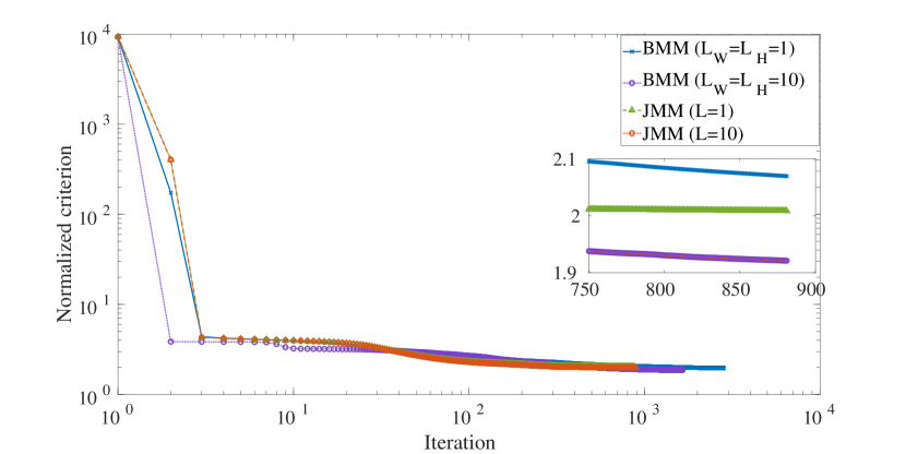
Figure 1: Impact of the number of sub-iterations in the minimization step of Algorithm 2. The box is a zoom-in on iterations $750$ to $881$. In the latter, BMM ($L_{W}=L_{H}=10$) and JMM ($L=10$) are overlapping.

As such, like in traditional NMF practice, in the following we only use one sub-iteration of $\mathbf{W}$ and $\mathbf{H}$ in our implementations of JMM and BMM. This means we set $L=1$ in Algorithm 2 and $L_{W}=L_{H}=1$ in Algorithm 1. By doing so, the BMM and JMM updates of $\mathbf{W}$ coincide and only the update of $\mathbf{H}$ changes (with still a significant gain in performance). Note that we have observed empirically that inverting the order of the updates in (9) does not have any impact on the number of iterations before convergence nor on the quality of the obtained solutions.

4.1.2 Initialization and stopping criterion

The initializations $(\mathbf{W}_{\text{init}},\mathbf{H}_{\text{init}})$ for BMM and JMM are drawn randomly according to a half-normal distribution. Our stopping criterion for both algorithms is based on the relative decrease in the objective function $D_{\beta}$. More precisely, the algorithms are stopped when

$$\frac{D_{\beta}(\mathbf{V}\mid\bar{\mathbf{W}}\bar{\mathbf{H}})-D_{\beta}(\mathbf{V}\mid\mathbf{W}\mathbf{H})}{D_{\beta}(\mathbf{V}\mid\mathbf{W}\mathbf{H})}\leq\epsilon\;,$$

where $\epsilon$ is a tolerance set to $10^{-5}$, $\mathbf{W}$ and $\mathbf{H}$ are the current outer-loop iterates while $\bar{\mathbf{W}}$ and $\bar{\mathbf{H}}$ are the previous ones (either $\bm{\check{\mathbf{W}}}$ and $\bm{\check{\mathbf{H}}}$ for BMM or $\bm{\tilde{\mathbf{W}}}$ and $\bm{\tilde{\mathbf{H}}}$ for JMM). Furthermore, in order to remove the scaling ambiguity inherent to NMF, we normalize $\mathbf{W}$ and $\mathbf{H}$ at the end of each outer-loop iteration for both BMM and JMM. The normalization consists in dividing each column of $\mathbf{W}$ by its $\ell_{2}$ norm and scaling the rows of $\mathbf{H}$ accordingly.

4.1.3 Handling zero values and numerical stability

The $\beta$-divergence $D_{\beta}(x|y)$ may not be defined when either $x$ or $y$ takes zero values. This is for instance the case when $\beta$ is set to $0$ or $1$ due to the quotient and the logarithm that appear. As such, we recommend minimizing $D_{\beta}(\mathbf{V}+\kappa\mathbf{1}|\mathbf{W}\mathbf{H}+\kappa\mathbf{1})$ with a small constant $\kappa$ instead of $D_{\beta}(\mathbf{V}|\mathbf{W}\mathbf{H})$ for numerical stability. This first simply amounts to replacing $\mathbf{V}$ by $\mathbf{V}+\kappa\mathbf{1}$ in the previous derivations. Then, by treating $\kappa$ as a ${(K+1)}^{\text{th}}$ constant component like in [27], we may simply replace the product $\bm{\tilde{\mathbf{W}}}\bm{\tilde{\mathbf{H}}}$ (resp. $\mathbf{W}\mathbf{H}$) by $\bm{\tilde{\mathbf{W}}}\bm{\tilde{\mathbf{H}}}+\kappa\mathbf{1}$ (resp. $\mathbf{W}\mathbf{H}+\kappa\mathbf{1}$) in (9) (resp. (5)).

4.1.4 Simulation environment

All the simulations have been conducted in Matlab 2020a running on an Intel i7-8650U CPU with a clock cycle of 1.90GHz shipped with 16GB of memory. In each of the following experimental scenarii, we compare the factorization obtained by JMM and BMM from $25$ different initializations $(\mathbf{W}_{\text{init}},\mathbf{H}_{\text{init}})$.

4.1.5 Performance evaluation

We compare BMM and JMM both in terms of computational efficiency (CPU time) and quality of the returned solutions. To assess the latter, we use the value of the normalized objective function $\frac{D_{\beta}(\mathbf{V}|\widehat{\mathbf{W}}\widehat{\mathbf{H}})}{FN}$ at the solution $(\widehat{\mathbf{W}},\widehat{\mathbf{H}})$ returned by the NMF algorithms. We also consider the KKT residuals [13] to measure the distance to the first order optimality conditions and attest whether the algorithms reached a critical point of the criterion $D_{\beta}$. The KKT residuals are expressed by

$$\text{res}(\mathbf{W}) =\frac{\left\lVert\min\{\mathbf{W},[{(\mathbf{W}\mathbf{H})}^{.(\beta-2)}.(\mathbf{W}\mathbf{H}-\mathbf{V})]\mathbf{H}^{\top}\}\right\rVert_{1}}{FK}$$

$$\text{res}(\mathbf{H}) =\frac{\left\lVert\min\{\mathbf{H},\mathbf{W}^{\top}[{(\mathbf{W}\mathbf{H})}^{.(\beta-2)}.(\mathbf{W}\mathbf{H}-\mathbf{V})]\}\right\rVert_{1}}{KN}\,.$$

4.2 Factorization of face images

In the context of image processing, NMF can be used to learn part-based features from a collection of images [1]. The columns of the matrix $\mathbf{V}$ correspond to the vectorization of the different images. Besides, the factor $\mathbf{W}$ represents the dictionary of image features, and the matrix $\mathbf{H}$ contains the activation encodings.

We compare the BMM and JMM methods on a face images dataset, the Olivetti dataset from AT&T Laboratories Cambridge [28], which contains $400$ greyscale images of faces with dimensions $64\times 64$. The corresponding matrix $\mathbf{V}$ thereby has dimensions $4096\times 400$. We set $K$ to $10$. We consider the values $0$, $1$, and $2$ for the parameter $\beta$, which correspond respectively to IS divergence, KL divergence, and squared Euclidean distance (the latter two being the most common in image processing).

Figure 2 shows the computation times for $\beta=2$ and $\beta=1$, as well as the values of the normalized objective function produced by both BMM and JMM, for the $25$ runs. The same random initialization is used by both methods. Note that we use a logarithmic scale for the CPU time and that the y-axis for the objective function does not start at zero. We observe that JMM is always faster than BMM while yielding solutions with a similar quality in terms of the objective $D_{\beta}$. The corresponding average CPU time as well as the resulting acceleration ratios are given in Table 4. We notice that the computational saving is higher when using the IS divergence, which confirms our analysis from Section 3.3.2. Remark that we measure here the global CPU time and not the time per iteration: since the auxiliary function is different for BMM and JMM, the trajectory in the parameter space is also different and thus the two algorithms do not require the same number of iterations before convergence. Nevertheless, we observe that the number of iterations for both algorithms has a similar order of magnitude. Since the iterations of JMM are cheaper, its global CPU time is lower. This remark also holds for higher dimensional dataset such as the one in Section 4.4.

Note that while MM algorithms are prevalent for $\beta$-NMF in general, many other algorithms have been designed for the specific case $\beta=2$ (quadratic loss) [8]. In that case, some algorithms are notoriously more efficient than BMM, see, e.g., [8, Chapter 8.2]. Though JMM improves on BMM, it may not compete with these other algorithms. Still, JMM, like BMM, is free of hyper-parameters and very easy to use, and remains a very convenient option for the general practitioner.

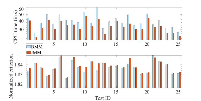
(a) Using KL divergence ($\beta=1$).

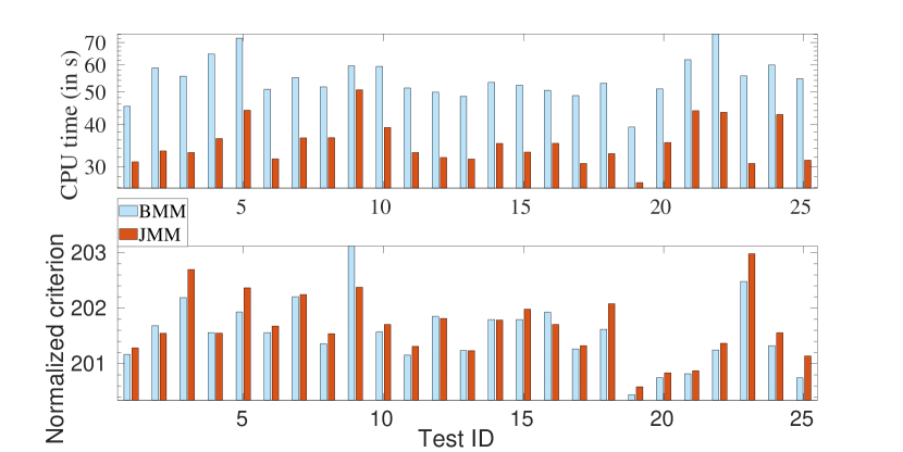
(b) Using quadratic loss ($\beta=2$).

Figure 2: Comparative performance using the Olivetti dataset ($K=10$).

Finally, we computed the KKT residuals for $\widehat{\mathbf{W}}$ and $\widehat{\mathbf{H}}$ returned by JMM and BMM, for all runs and considered values of $\beta$. We observed that they range from $1.10^{-5}$ to $1.10^{-1}$, indicating that both methods converge to a critical point of $D_{\beta}$. As a matter of fact, an additional significant observation is that in all cases here, both JMM and BMM return the same solution $(\hat{\mathbf{W}},\hat{\mathbf{H}})$ up to permutation of their columns and up to some round-off errors. Nevertheless, the trajectory of the iterates may differ.

4.3 Factorization of a spectrogram

We now consider NMF of audio magnitude spectrograms. In this context the factor $\mathbf{W}$ contains elementary audio spectra with temporal activations given by $\mathbf{H}$ [2].

We generate the spectrogram of an excerpt from the original recording of the song “Four on Six” by Wes Montgomery. The signal is $50$-seconds long with a sampling rate of $44.1\text{\,}\mathrm{kHz}$. The spectrogram is computed with a Hamming window of length $2048$ (46ms) and an overlap of $50\%$. This results in a data matrix $\mathbf{V}$ of dimensions $1025\times 2152$.

In this section, we set $\beta=0$, which is a common value in audio signal processing [29], and set $K$ to $10$. The results obtained with BMM and JMM are shown on Figure 3. The average computation time for BMM is 291s while the one for JMM is 41s, which yields an average acceleration of $86\%$. We observe a very substantial benefit of JMM over BMM in terms of CPU time in this case. This confirms our conclusion from Section 3.3.2 that JMM reaches its highest potential with NMF based on the IS divergence. We observe here again that JMM and BMM return the same solution $(\hat{\mathbf{W}},\hat{\mathbf{H}})$ up to permutation of their columns.

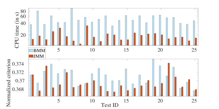
Figure 3: Comparative performance with a spectrogram
                                                                                                                                                 ($K=10,\beta=0$).

4.4 Factorization of song play-counts

NMF may be used in recommendation systems based on implicit user data. In this case, the matrix $\mathbf{V}$ contains information about the interactions of users with a collection of items. The factor $\mathbf{W}$ may extract user preferences while $\mathbf{H}$ represents item attributes, see, e.g., [5].

We here consider the TasteProfile dataset [30] which contains counts of songs played by users (e.g., of a music streaming service). Similarly to [31] and many other papers using this dataset, we apply a preprocessing to the original data to keep only users and songs with more than a given number of interactions (here set to 20). This results in a large and sparse data matrix $\mathbf{V}$ of dimensions $16\,301\times 12\,118$ with about $0.6\%$ nonzero values. We set $\beta$ to $1$ (a common choice in recommender systems, because its corresponds to the log-likelihood of a Poisson model that is natural for count data), and $K=50$.

Comparative results are displayed in Figure 4. We observe that on average, JMM is $13\%$ faster with an average CPU time of 1 hour 38 minutes whereas BMM’s average time is equal to 1 hour 58 minutes. Finally, like in previous scenarii, JMM and BMM return the same solution $(\hat{\mathbf{W}},\hat{\mathbf{H}})$ up to a permutation of their columns.

Similarly to our observations of Section 4.2, we observe that, while BMM has generally a shorter trajectory than BMM, the number of iterations of both methods has the same order of magnitude. Since the cost of BMM per iteration is higher than JMM, this results in a higher overall CPU time.

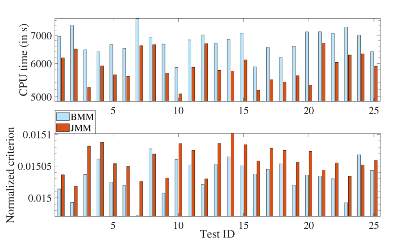
Figure 4: Comparative performance with TasteProfile
                                                                                                                                                 ($K=50,\beta=1$).

4.5 Factorization of hyperspectral images

A hyperspectral image is a multi-band image that can be represented by a nonnegative matrix: each row represents a spectral band while each column represents a pixel of the image. Applying NMF to such matrix data allows extracting a collection of individual spectra representing the different materials arranged in the matrix $\mathbf{W}$, as well as their relative proportions given by the matrix $\mathbf{H}$, see, e.g., [4].

We consider a hyperspectral image acquired over Moffett Field in 1997 by the Airborne Visible Infrared Imaging Spectrometer [32]. The image contains $50\times 50$ pixels over $189$ spectral bands, which leads to a matrix $\mathbf{V}$ of dimensions $189\times 2500$. We consider $\beta=2$ and $\beta=1.5$. The latter value in particular was shown to be an interesting trade-off between Poisson ($\beta=1$) and additive Gaussian ($\beta=2$) assumptions for predicting missing values in incomplete versions of this dataset, see [27]. The factorization rank $K$ is set to $3$, a standard choice with this dataset (extraction of vegetation, soil and water).

Comparative results are given in Figure 5. On the top figure corresponding to $\beta=2$, we observe that JMM is faster than BMM with an acceleration of $31\%$ on average. On the other hand, for $\beta=1.5$, we observe that BMM is faster in general (though not always). This confirms again our analysis in Section 3.3.2: when $\beta$ is different from $0$, $1$, and $2$, the benefit of JMM may be counterbalanced by the additional divisions in the general formulae (9).

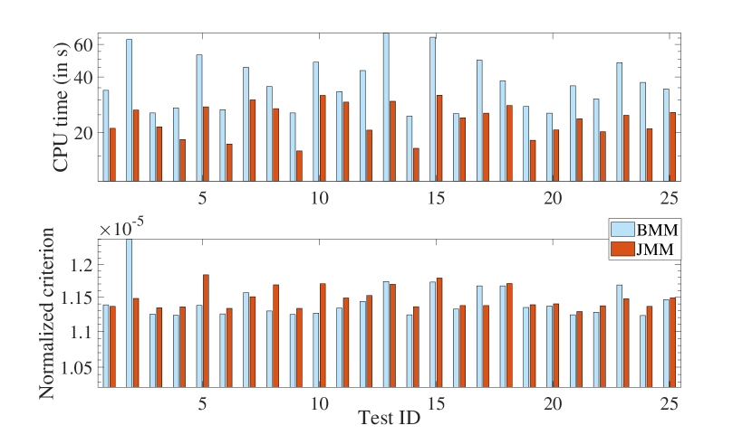
(a) $\beta=2$.

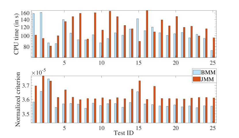
(b) $\beta=1.5$.

Figure 5: Comparative performance with Moffet hyperspectral image ($K=3$).

4.6 Summary of the experiments

Table 4 summarizes the average and the standard deviation of the CPU times for all the datasets considered. It can be observed that JMM yields a significant speed-up for the widely used settings when $\beta$ equals to $0$, $1$, or $2$. This acceleration is observed on small, medium and large size datasets. The corresponding $95\%$ confidence intervals are given in Table 5.

Table 4: Summary for the statistics on CPU times and the acceleration in all the tested dataset. The displayed values are the averages while the standard deviations are indicated within parenthesis.

	BMM	JMM	Acc.
Olivetti ($\beta=2$)	55s (8s)	36s (6s)	35%
Olivetti ($\beta=1$)	40s (9s)	34s (6s)	16%
Olivetti ($\beta=0$)	229s (32s)	63s (8s)	72%
Spectrogram ($\beta=0$)	291s (90s)	41s (8s)	86%
TasteProfile ($\beta=1$)	6776s (439s)	5909s (492s)	13%
Moffet ($\beta=2$)	39s (13s)	24s (5s)	35%
Moffet ($\beta=1.5$)	107s (22s)	123s (26s)	-18%

Table 5: The $95\%$ confidence intervals for the CPU times of BMM and JMM (in seconds).

	BMM	JMM
Olivetti ($\beta=2$)	$[52,58]$	$[34,38]$
Olivetti ($\beta=1$)	$[36,44]$	$[32,36]$
Olivetti ($\beta=0$)	$[216,242]$	$[60,66]$
Spectrogram ($\beta=0$)	$[254,328]$	$[38,43]$
TasteProfile ($\beta=1$)	$[6595,6957]$	$[5706,6112]$
Moffet ($\beta=2$)	$[34,44]$	$[22,26]$
Moffet ($\beta=1.5$)	$[98,116]$	$[112,133]$

5 Conclusion

In this paper, we have presented a joint MM method for NMF with the $\beta$-divergence. Our algorithm relies on the alternating minimization of a non-convex auxiliary function and leads to new multiplicative updates of the factor matrices. These new updates are variants of the classic multiplicative updates and are equally simple to implement. They can lead to a significant computational speedup, especially for the Itakura-Saito and Kullback Leibler divergences, and the quadratic loss. Fortunately, the three later cases are the three most common cases of NMF with the $\beta$-divergence. The new updates guarantee the descent property for the objective function. Moreover, we have observed experimentally that the estimated factors are of the same quality as the ones returned by the classic block MM scheme. As a matter of fact, we have noted that both algorithms usually return the same solutions up to column permutation. The computational efficiency of the proposed updates has been demonstrated on datasets with diverse characteristics. In future work, we intend to study the convergence of the iterates of JMM. This is a challenging topic because of the non-convexity of the majorizer which underpins our approach. Such a difficulty explains the scarcity of results in the literature on the convergence of MM algorithms with non-convex auxiliary functions. Another promising topic would consist in designing stochastic versions of JMM for the factorization of massive datasets [33, 34].

References

- [1] D. D. Lee, H. S. Seung, Learning the parts of objects by non-negative matrix factorization, Nature 401 (6755) (1999) 788–791. doi:10.1038/44565.
- [2] P. Smaragdis, C. Févotte, G. J. Mysore, N. Mohammadiha, M. Hoffman, Static and dynamic source separation using nonnegative factorizations: A unified view, IEEE Signal Process. Mag. 31 (3) (2014) 66–75. doi:10.1109/msp.2013.2297715.
- [3] M. W. Berry, M. Browne, A. N. Langville, V. P. Pauca, R. J. Plemmons, Algorithms and applications for approximate nonnegative matrix factorization, Comput. Stat. Data Anal. 52 (1) (2007) 155–173. doi:10.1016/j.csda.2006.11.006.
- [4] J. M. Bioucas-Dias, A. Plaza, N. Dobigeon, M. Parente, Q. Du, P. Gader, J. Chanussot, Hyperspectral unmixing overview: Geometrical, statistical, and sparse regression-based approaches, IEEE J. Sel. Top. Appl. Earth Obs. Remote Sens. 5 (2) (2012) 354–379. doi:10.1109/jstars.2012.2194696.
- [5] Y. Hu, Y. Koren, C. Volinsky, Collaborative filtering for implicit feedback datasets, in: Proc. IEEE Int. Conf. Data Mining, IEEE, 2008. doi:10.1109/icdm.2008.22.
- [6] A. Cichocki, R. Zdunek, A. H. Phan, Nonnegative Matrix and Tensor Factorizations: Applications to Exploratory Multi-Way Data Analysis and Blind Source Separation, John Wiley & Sons Inc, 2009. doi:10.1002/9780470747278.
- [7] X. Fu, K. Huang, N. D. Sidiropoulos, W.-K. Ma, Nonnegative matrix factorization for signal and data analytics: Identifiability, algorithms, and applications, IEEE Signal Process. Mag. 36 (2) (2019) 59–80. doi:10.1109/msp.2018.2877582.
- [8] N. Gillis, Nonnegative Matrix Factorization, Society for Industrial and Applied Mathematics, 2020. doi:10.1137/1.9781611976410.
- [9] A. Cichocki, S. Cruces, S. ichi Amari, Generalized Alpha-Beta divergences and their application to robust nonnegative matrix factorization, Entropy 13 (1) (2011) 134–170. doi:10.3390/e13010134.
- [10] D. D. Lee, H. S. Seung, Algorithms for non-negative matrix factorization, in: Adv. Neural and Inform. Process. Syst., Vol. 13, 2001, pp. 556–562.
- [11] R. Kompass, A generalized divergence measure for nonnegative matrix factorization, Neural Comput. 19 (3) (2007) 780–791. doi:10.1162/neco.2007.19.3.780.
- [12] M. Nakano, H. Kameoka, J. L. Roux, Y. Kitano, N. Ono, S. Sagayama, Convergence-guaranteed multiplicative algorithms for nonnegative matrix factorization with -divergence, in: IEEE Int. Workshop Mach. Learn. Signal Process., IEEE, 2010. doi:10.1109/mlsp.2010.5589233.
- [13] C. Févotte, J. Idier, Algorithms for nonnegative matrix factorization with the -divergence, Neural Comput. 23 (9) (2011) 2421–2456. doi:10.1162/neco\_a\_00168.
- [14] Z. Yang, E. Oja, Unified development of multiplicative algorithms for linear and quadratic nonnegative matrix factorization, IEEE Trans. Neural Netw. 22 (12) (2011) 1878–1891. doi:10.1109/tnn.2011.2170094.
- [15] K. Lange, MM Optimization Algorithms, Society for Industrial and Applied Mathematics, 2016. doi:10.1137/1.9781611974409.
- [16] Y. Sun, P. Babu, D. P. Palomar, Majorization-minimization algorithms in signal processing, communications, and machine learning, IEEE Trans. Signal Process. 65 (3) (2017) 794–816. doi:10.1109/tsp.2016.2601299.
- [17] A. Rakotomamonjy, Direct optimization of the dictionary learning problem, IEEE Trans. Signal Process. 61 (22) (2013) 5495–5506. doi:10.1109/tsp.2013.2278158.
- [18] M. C. Mukkamala, P. Ochs, Beyond alternating updates for matrix factorization with inertial Bregman proximal gradient algorithms, in: H. Wallach, H. Larochelle, A. Beygelzimer, F. d'Alché-Buc, E. Fox, R. Garnett (Eds.), Proc. Ann. Conf. Neur. Inform. Proc. Syst., Vol. 32, Curran Associates, Inc., 2019.
- [19] J. Bolte, S. Sabach, M. Teboulle, Y. Vaisbourd, First order methods beyond convexity and Lipschitz gradient continuity with applications to quadratic inverse problems, SIAM J. Optim. 28 (3) (2018) 2131–2151. doi:10.1137/17M1138558.
- [20] I. Panageas, S. Skoulakis, A. Varvitsiotis, X. Wang, Convergence to second-order stationarity for non-negative matrix factorization: Provably and concurrently, arXiv preprint: arxiv.org/abs/2002.11323 (2020). arXiv:2002.11323.
- [21] N. Marumo, T. Okuno, A. Takeda, Majorization-minimization-based Levenberg-Marquardt method for constrained nonlinear least squares, Comput. Optim. Appl. 84 (3) (2023) 833–874. doi:10.1007/s10589-022-00447-y.
- [22] M. Vandecappelle, N. Vervliet, L. D. Lathauwer, A second-order method for fitting the canonical polyadic decomposition with non-least-squares cost, IEEE Trans. Signal Process. 68 (2020) 4454–4465. doi:10.1109/tsp.2020.3010719.
- [23] N. Takahashi, J. Katayama, M. Seki, J. Takeuchi, A unified global convergence analysis of multiplicative update rules for nonnegative matrix factorization, Comput. Optim. Appl. 71 (1) (2018) 221–250. doi:10.1007/s10589-018-9997-y.
- [24] R. Zhao, V. Y. F. Tan, A unified convergence analysis of the multiplicative update algorithm for regularized nonnegative matrix factorization, IEEE Trans. Signal Process. 66 (1) (2018) 129–138. doi:10.1109/tsp.2017.2757914.
- [25] M. Razaviyayn, M. Hong, Z.-Q. Luo, A unified convergence analysis of block successive minimization methods for nonsmooth optimization, SIAM J. Optim. 23 (2) (2013) 1126–1153. doi:10.1137/120891009.
- [26] K. Lange, Optimization, Springer New York, 2013. doi:10.1007/978-1-4614-5838-8.
- [27] C. Févotte, N. Dobigeon, Nonlinear hyperspectral unmixing with robust nonnegative matrix factorization, IEEE Trans. Image Process. 24 (12) (2015) 4810–4819. doi:10.1109/tip.2015.2468177.
- [28] F. S. Samaria, A. Harter, Parameterisation of a stochastic model for human face identification, in: Proc. Workshop on Applications of Computer Vision, IEEE Comput. Soc. Press, 1994. doi:10.1109/acv.1994.341300.
- [29] C. Févotte, N. Bertin, J.-L. Durrieu, Nonnegative matrix factorization with the Itakura-Saito divergence: With application to music analysis, Neural Comput. 21 (3) (2009) 793–830. doi:10.1162/neco.2008.04-08-771.
- [30] T. Bertin-Mahieux, D. P. Ellis, B. Whitman, P. Lamere, The million song dataset, in: Proc. Int. Conf. Music Inform. Retrieval (ISMIR), 2011.
- [31] O. Gouvert, T. Oberlin, C. Févotte, Ordinal non-negative matrix factorization for recommendation, in: Proc. Int. Conf. Mach. Learn., 2020, pp. 3680–3689.
-
[32]
Jet Propulsion Lab (JPL),
Aviris free
data, california Inst. Technol., Pasadena, CA (2006).
URL http://aviris.jpl.nasa.gov/html/aviris.freedata.html - [33] A. Mensch, J. Mairal, B. Thirion, G. Varoquaux, Stochastic subsampling for factorizing huge matrices, IEEE Trans. Signal Process. 66 (1) (2018) 113–128. doi:10.1109/tsp.2017.2752697.
- [34] W. Pu, S. Ibrahim, X. Fu, M. Hong, Stochastic mirror descent for low-rank tensor decomposition under non-Euclidean losses, IEEE Trans. Signal Process. 70 (2022) 1803–1818. doi:10.1109/tsp.2022.3163896.