Asymptotic Log-Det Sum-of-Ranks Minimization via Tensor (Alternating) Iteratively Reweighted Least Squares

Abstract.

Affine sum-of-ranks minimization (ASRM) generalizes the affine rank minimization (ARM) problem from matrices to tensors. Here, the interest lies in the ranks of a family $\mathcal{K}$ of different matricizations. Transferring our priorly discussed results on asymptotic log-det rank minimization, we show that iteratively reweighted least squares with weight strength $p=0$ remains a, theoretically and practically, particularly viable method denoted as IRLS-$0\mathcal{K}$. As in the matrix case, we prove global convergence of asymptotic minimizers of the log-det sum-of-ranks function to desired solutions. Further, we show local convergence of IRLS-$0\mathcal{K}$ in dependence of the rate of decline of the therein appearing regularization parameter $\gamma\searrow 0$. For hierarchical families $\mathcal{K}$, we show how an alternating version (AIRLS-$0\mathcal{K}$, related to prior work under the name SALSA) can be evaluated solely through tensor tree network based operations. The method can thereby be applied to high dimensions through the avoidance of exponential computational complexity. Further, the otherwise crucial rank adaption process becomes essentially superfluous even for completion problems. In numerical experiments, we show that the therefor required subspace restrictions and relaxation of the affine constraint cause only a marginal loss of approximation quality. On the other hand, we demonstrate that IRLS-$0\mathcal{K}$ allows to observe the theoretical phase transition also for generic tensor recoverability in practice. Concludingly, we apply AIRLS-$0\mathcal{K}$ to larger scale problems.

Key words. affine rank minimization, iteratively reweighted least square, matrix recovery, matrix completion, log-det function

AMS subject classifications. 15A03, 15A29, 65J20, 90C31, 90C26

1. Introduction

The setting of affine sum-of-ranks minimization (ASRM) is a generalization of the affine rank minimization (ARM) problem for matrices to tensors. While the tensor rank refers to the minimal number of elementary tensors required for a decomposition into a sum, we are here interested in the ranks of so called matricizations. Let $[d]=\{1,\ldots,d\}$, $d\in\mathbb{N}$, as well as $n_{\mu}\in\mathbb{N}$, $\mu=1,\ldots,d$. For $\emptyset\neq J\subsetneq[d]$ and $J^{\mathsf{c}}:=[d]\setminus J$, we define such matricizations (cf. [15])

$$(\cdot)^{[J]}:\mathbb{R}^{n_{1}}\otimes\ldots\otimes\mathbb{R}^{n_{d}}\rightarrow\mathbb{R}^{n_{J}\times n_{J^{\mathsf{c}}}},\quad n_{S}:=\prod_{\mu\in S}n_{\mu},$$

as the simple reshaping isomorphisms induced via

$$(v_{1}\otimes\ldots\otimes v_{d})^{[J]}:=\mathrm{vec}(\bigotimes_{j\in J}v_{j})\cdot\mathrm{vec}(\bigotimes_{j\in J^{\mathsf{c}}}v_{j})^{T},\quad v_{i}\in\mathbb{R}^{n_{i}},\ i=1,\ldots,d,$$

where $\mathrm{vec}(\cdot):\mathbb{R}^{\bigtimes_{\mu\in S}n_{\mu}}\rightarrow\mathbb{R}^{n_{S}}$ denotes the vectorization in co-lexicographic (column-wise) order. As usual, we identify $\mathbb{R}^{n_{1}}\otimes\ldots\otimes\mathbb{R}^{n_{d}}\cong\mathbb{R}^{n_{1}\times\ldots\times n_{d}}$. For a (not necessarily hierarchical) family of subsets $\mathcal{K}\subseteq\{J\subsetneq[d]\mid J\neq\emptyset\}$ and a surjective linear operator $\mathcal{L}:\mathbb{R}^{n_{1}\times\ldots\times n_{d}}\rightarrow\mathbb{R}^{\ell}$, $\ell<n_{[d]}$, as well as measurements $y\in\mathrm{image}(\mathcal{L})$, we then define ASRM to refer to the problem of finding

(1.1) $$\underset{X\in\mathbb{R}^{n_{1}\times\ldots\times n_{d}}}{\mathrm{argmin}}\sum_{J\in\mathcal{K}}\mathrm{rank}(X^{[J]})\quad\mbox{subject to }\mathcal{L}(X)=y.$$

This setting is not only of particular interest due to its regularizing properties, but its close relation to so called hierarchical (or tensor tree) decompositions (cf. [15, 25]). We are here however mainly interested in the problem itself, and only secondarily in the possibility to recover an eventual ground truth tensor from its measurements. As large parts of this work rely on our preceding article [26], which in turn is based on [29, 11, 5, 7], we strongly recommend to take notice of such.

1.1. Approaches to ASRM and tensor recovery

Affine rank minimization (ARM), as theoretical origin of ASRM, is included as such for the dimension $d=2$ and $\mathcal{K}=\{\{1\}\}$ [26], and consequently defined as the problem to find a matrix

$$X^{\ast}\in\underset{X\in\mathbb{R}^{n\times m}}{\mathrm{argmin}}\ \mathrm{rank}(X)\quad\mbox{subject to }\mathcal{L}(X)=y.$$

This setting in turn is based on the affine cardinality minimization problem (ACM), that is to find a vector

$$x^{\ast}\in\underset{x\in\mathbb{R}^{n}}{\mathrm{argmin}}\ \mathrm{card}(x)\quad\mbox{subject to}\quad\mathcal{L}(x)=y.$$

A short overview over recovery methods as well as the role of iteratively reweighted least squares (IRLS, cf. [29, 11] for ARM and [5, 7] for ACM) for these two problems can be found in our preceding article [26]. To the best of our knowledge, IRLS has only priorly been considered with regard to the ASRM problem for tensors in the thesis [25], from which also the related, so called stable ALS approximation algorithm [16] stems. Relaxations of ASRM itself however have been considered before, including the minimization of the sum of nuclear norms [12, 28, 35]. The tensor rank as outlined in the introduction, Section 1, however, is hard to calculate, and usually not the direct target of minimization. Though [38, 37] utilize the canonical polyadic decomposition to a certain fiber completion problem. Other algorithm rely on the explicit, separate adaption of unknown ranks such as low rank manifold [39, 27, 36] or a-priorly representation or subspace based optimization [19, 18, 34]. However, non-intrusive rank adaption schemes, even if elaborate, tend to be problematic [16]. The AIRLS related method presented therein, as well as [13, 2, 14] based thereon, contrarily consider an intrusive regularization related to reweighting that circumvents the instability and overfitting problems otherwise caused. Another class of algorithm requires to choose specific sampling points, prominently cross approximation based methods [1, 31, 22]. Though such are preferable in that setting, we here however assume the affine measurement operator to be a priorly given.

1.2. Contributions and organization of this paper

The novel aspects of this paper are organized as follows.

• In Sections 1.3 and 1.4, we generalize the optimization as well as reweighting process from the matrix to the tensor case in an introductory manner. Section 1.5 contains a preliminary description of hierarchical decompositions and the thereto related data sparse optimization.

• In Section 2, we interpret the tensor log-det approach as successive minimization scheme and thereby prove the convergence of global optima to the desired solution, as analogously done for the matrix case [26].

• Section 3 provides global convergence results for the adjusted tensor IRLS-$0\mathcal{K}$ algorithm with respect to sequences of complementary weights, under consideration of the rate of decline of the regularization parameter $\gamma$.

• In Section 4, we discuss the relaxation of the affine constraint together with the restriction to iteratively defined sequences of admissible subspaces.

• Section 5 concisely reintroduces hierarchical formats as non-rooted tree tensor networks with an emphasis on its graph theoretical foundation. It contains several fundamental statements required for the subsequently introduced A(lternating)IRLS-$0\mathcal{K}$ algorithm.

• In Section 6, we utilize tree tensor networks to derive the AIRLS-$0\mathcal{K}$ algorithm which allows a non-exponentially scaling realization of the relaxed IRLS-$0\mathcal{K}$ method introduced in Section 4 through an evaluation within given low rank representations.

• Section 7 contains a comprehensive series of numerical experiments. Firstly, we demonstrate that IRLS-$0\mathcal{K}$ allows to observe the theoretical phase transition [4] regarding the required number of measurements for recoveries. Secondly, we follow the relaxations laid out in this work made from IRLS-$0\mathcal{K}$ up to the AIRLS-$0\mathcal{K}$ approach. We demonstrate the improvement, but likewise common ground towards our priorly introduced, so called SALSA algorithm [16], as well as superiority over conventional ALS. We conclude with an application of AIRLS-$0\mathcal{K}$ to large scale problems in higher dimensions.

• Appendix A contains a postponed proof. The supplementary Appendix SM1 includes a further numerical experiment. Appendix SM3 contains extended visualization of results as explained in Appendix SM2. Technical proofs concerning branch evaluations and therefor partially necessary notation can be found in Appendices SM4 and SM5. The AIRLS-$0\mathcal{K}$ method is summarized in Section SM5.4, whereas Appendix SM6 discusses viable heuristics.

1.3. Asymptotic minimization

We have priorly discussed in [26] as based on [29, 11, 5, 7] in which way the ARM problem for matrices can be approached via the asymptotic minimization (cf. Definition 1.1) of the family

(1.2) $$f_{\gamma}(A):=\log\prod_{i=1}^{k_{1}}(\sigma_{i}^{2}(A)+\gamma)=\log\det(AA^{T}+\gamma I),\quad\gamma\searrow 0,$$

for which $\sigma_{i}(A)$, $i=1,\ldots,r$, are defined as the singular values of $A\in\mathbb{R}^{k_{1}\times k_{2}}$ and $\sigma_{i}(A)=0$, $i>r$, $r=\mathrm{rank}(A)$. Plainly analogous, its tensor version for the minimization of a sum of ranks is defined as (see Section 2)

(1.3) $$f^{\mathcal{K}}_{\gamma}(X):=\sum_{J\in\mathcal{K}}f_{\gamma}(X^{[J]})=\log\prod_{J\in\mathcal{K}}\prod_{i=1}^{n_{J}}(\sigma_{i}^{(J)}(X)^{2}+\gamma),$$

where $\sigma_{i}^{(J)}(X)=\sigma_{i}(X^{[J]})$ is the $i$-th singular value of the matrix $X^{[J]}\in\mathbb{R}^{n_{J}\times n_{J^{\mathsf{c}}}}$. Thus the matrix version corresponds to $\mathcal{K}=\{\{1\}\}$, whereas for the alternating IRLS method, we have also considered the complementary $\mathcal{K}=\{\{2\}\}$. In [26], we have already reasoned the choice $p=0$ of the therein appearing weight strength parameter $p\in[0,1]$. Thus, we here only regard the thereto corresponding log-det approach laid out above, as opposed to the other extreme $p=1$ associated to nuclear norm minimization. This leads us to the following, potential solutions to the ASRM problem.

Definition 1.1.

We define

$$\mathcal{X}^{\ast}:=\{X^{\ast}\mid\exists(X_{\gamma})_{\gamma>0}\subset\mathcal{L}^{-1}(y),\ X^{\ast}=\lim_{\gamma\searrow 0}X_{\gamma},\ f^{\mathcal{K}}_{\gamma}(X_{\gamma})=\min_{X\in\mathcal{L}^{-1}(y)}f^{\mathcal{K}}_{\gamma}(X)\}.$$

This set of asymptotic, global minimizers indeed yields the desired solutions as we prove in Theorem 2.4. The decline of the parameter $\gamma$ is no less important here as more detailly remarked on in the predecessor [26]. It should further be noted that neither the ranks $r^{(J)}:=\mathrm{rank}(X^{[J]})$ (cf. Section 2), nor the families of singular values $\sigma^{(J)}$, $J\in\mathcal{K}$, are independent of each other [24], though not prohibitively so in regard of aboves approach.

1.4. Iteratively reweighted least squares (IRLS)

In line with the overall generalization, also iteratively reweighted least squares (IRLS) allows to be applied to the minimization of a sum of ranks of a tensor. For the matrix case, one version (cf. [26, 29]) defines ($\|\cdot\|_{F}$ being the Frobenius norm)

$$X^{(i)}:=\underset{X\in\mathcal{L}^{-1}(y)}{\mathrm{argmin}}\ \|W_{\gamma^{(i-1)},X^{(i-1)}}^{1/2}X\|_{F},\quad W_{\gamma,X}:=(XX^{T}+\gamma I)^{-1},$$

for a monotonically decreasing sequence $\{\gamma^{(i)}\}_{i\geq 0}\subset\mathbb{R}_{>0}$. The tensor variant straightforwardly is given by (see Section 3)

(1.4) $$X^{(i)} :=\underset{X\in\mathcal{L}^{-1}(y)}{\mathrm{argmin}}\sum_{J\in\mathcal{K}}\big{\|}(W^{(J)}_{\gamma^{(i-1)},X^{(i-1)}})^{1/2}(X^{(i)})^{[J]}\big{\|}_{F}^{2},$$

where the weight matrices follow the same generalization with

$$W^{(J)}_{\gamma,X} :=W_{\gamma,X^{[J]}}=\big{(}X^{[J]}(X^{[J]})^{T}+\gamma I\big{)}^{-1},\quad J\in\mathcal{K}.$$

Continued from the vector as well as matrix case, it also here holds true that for a sequence $X_{\gamma}\rightarrow\overline{X}$ with sufficiently fast declining singular values

$$\sum_{J\in\mathcal{K}}\big{\|}W^{(J)}_{\gamma,X_{\gamma}}X^{[J]}_{\gamma}\big{\|}^{2}_{F}=\sum_{J\in\mathcal{K}}\sum_{i=1}^{n_{J}}\frac{\sigma^{(J)}_{i}(X_{\gamma})^{2}}{\sigma^{(J)}_{i}(X_{\gamma})^{2}+\gamma}\underset{\gamma\searrow 0}{\longrightarrow}\sum_{J\in\mathcal{K}}\mathrm{rank}(\overline{X}^{[J]}).$$

Though largely similar to the matrix case, there is however at least one difference as we discuss in Section 2. Due to its dependence on $p=0$ and the family $\mathcal{K}$, we abbreviate aboves algorithm 1.4 as IRLS-$0\mathcal{K}$.

1.5. Data sparse optimization

With increasing dimensions $d$, the size of the space $\mathbb{R}^{n_{1}\times\ldots\times n_{d}}$ quickly becomes prohibitively large. While for smaller instances, IRLS-$0\mathcal{K}$ is by all means a viable algorithm, it otherwise remains a theoretical ideal. However, for hierarchical families $\mathcal{K}$, that is if

(1.5) $$(J\subset S\quad\vee\quad S\subset J\quad\vee\quad J\cap S=\emptyset)\quad\wedge\quad J\neq S^{\mathsf{c}},\qquad\forall J,S\in\mathcal{K},$$

so called hierarchical decompositions [15] or, basically synonymously, tensor tree networks (cf. [10, 25]) provide remedy in the same way the ordinary low rank matrix decomposition does (cf. [26]). In the latter case, the data space $\mathcal{D}_{r}:=\{(Y,Z)\mid Y\in\mathbb{R}^{k_{1}\times r},\ Z\in\mathbb{R}^{r\times k_{2}}\}$ represents the low rank variety

$$V^{k_{1},k_{2}}_{\leq r}:=\{A\in\mathbb{R}^{k_{1}\times k_{2}}\mid\mathrm{rank}(A)\leq r\}$$

via the surjective (but not injective) bilinear map

(1.6) $$\tau_{r}:\mathcal{D}_{r}\rightarrow V_{\leq r},\quad\tau_{r}(Y,Z):=YZ\in\mathbb{R}^{n_{1}\times n_{2}}.$$

The alternating method AIRLS then only requires to operate on $\mathcal{D}_{r}$, while directly minimizing $f_{\gamma}$ subject to relaxed affine constraints (see Section 4). In the tensor case, where the rank becomes $r=\{r^{(J)}\}_{J\in\mathcal{K}}\in\mathbb{N}^{\mathcal{K}}$, the variety

(1.7) $$V^{\mathcal{K}}_{\leq r}:=\{X\in\mathbb{R}^{n_{1}\times\ldots\times n_{d}}\mid X^{[J]}\in V^{n_{J},n_{J^{\mathsf{c}}}}_{\leq r^{(J)}},\ J\in\mathcal{K}\},$$

has a logarithmicly lower dimension and is likewise represented by a data space $\mathcal{D}_{r}$ together with a simple, surjective and multilinear contraction map $\tau_{r}:\mathcal{D}_{r}\rightarrow V^{\mathcal{K}}_{\leq r}$ (see Section 5). Thereby, a sparse optimization as for matrices is also possible in higher dimensions. Ultimately, also AIRLS-$0\mathcal{K}$ (see Section 6) distinguishes itself from well known unregularized alternating least squares (ALS) [20] only through an additional penalty term. However, it thereby not only becomes stable by means of [16], but it is derived from and directly minimizes the objective function $f^{\mathcal{K}}_{\gamma}$ restricted to $V^{\mathcal{K}}_{\leq r}$.

2. Underlying structure and global behavior

Phrased more generalized, we in principle desire to solve the problem (cf. [26]) of finding

(2.1) $$X^{\ast}\in\underset{X\in\mathcal{L}^{-1}(y)}{\mathrm{argmin}}\ \mathcal{C}_{\mathcal{V}}(X),\quad\mathcal{C}_{\mathcal{V}}(v):=\min_{V\in\mathcal{V}:\ X\in V}\mathrm{dim}(V),$$

where in this setting the family of varieties $\mathcal{V}$ is

$$\mathcal{V}_{d}^{\mathcal{K}}:=\{V^{\mathcal{K}}_{\leq r}\subset\mathbb{R}^{n_{1}\times\ldots\times n_{d}}\mid r=\{r^{(J)}\}_{J\in\mathcal{K}}\in\mathbb{N}_{0}^{\mathcal{K}}\},$$

for $V^{\mathcal{K}}_{\leq r}$ as defined in 1.7. In general however, the dimension of $V^{\mathcal{K}}_{\leq r}$ does not equal $\sum_{J\in\mathcal{K}}r^{(J)}$, and is thus not directly represented by the sum of ranks as in 1.1. While

$$V^{\mathcal{K}}_{\leq\widetilde{r}}\subsetneq V^{\mathcal{K}}_{\leq r}\quad\Rightarrow\quad\widetilde{r}^{(J)}\leq r^{(J)},\ J\in\mathcal{K},\ \widetilde{r}\neq r\quad\Rightarrow\quad\dim(\mathcal{V}^{\mathcal{K}}_{\leq\widetilde{r}})<\dim(\mathcal{V}^{\mathcal{K}}_{\leq r}),$$

neither of the converse implications holds true in general. Firstly, some differently indexed varieties are equal since some constellations $r\in\mathbb{N}_{0}^{\mathcal{K}}$ are unfeasible [25].

Definition 2.1.

The values $r=\{r^{(J)}\}_{J\in\mathcal{K}}$ are called (un)feasible (for $n\in\mathbb{N}^{d}$), if there exists (not) at least one tensor $X\in\mathbb{R}^{n_{1}\times\ldots\times n_{d}}$ with $\mathrm{rank}(X^{[J]})=r^{(J)}$, $J\in\mathcal{K}$.

For hierarchical sets $\mathcal{K}$, these bounds are (cf. [25]) $r^{(J_{\hat{e}})}\leq n_{v}\prod_{e\in E_{v}\setminus\{\hat{e}\}}r^{(J_{e})}$ for $\hat{e}\in E_{v}$, $v\in V$. This natural interrelation of ranks is somewhat beneficial to the simplified sum-of-ranks approach as it excludes some extremal cases. The sum-of-ranks minimization is itself a necessary relaxation of the (arguably) more desirable objective function $\mathcal{C}_{\mathcal{V}^{\mathcal{K}}_{d}}$, yet it is closer than it might first seem. What remains however is that, contrarily to the matrix case, the varieties are only partially nested.

2.1. Determinant expansion and convergence of (global) minimizers

Following from the matrix case, one can likewise expand the function $f_{\gamma}^{\mathcal{K}}$ into squared sums of minors defined as

$$\mathrm{det}^{2}_{k}(A) :=\sum_{I\in\mathcal{P}_{k}([n_{J}])}\sum_{J\in\mathcal{P}_{k}([n_{J^{\mathsf{c}}}])}\det(A_{I,J})^{2},\quad k=1,\ldots,n_{J},$$

for $A_{I,J}:=\{A_{i,j}\}_{i\in I,j\in J}\in\mathbb{R}^{|I|\times|J|}$ and $\mathcal{P}_{k}([\ell]):=\{I\subseteq\{1,\ldots,\ell\}\mid|I|=k\}$. For simplicity of notation, we further define $\mathrm{det}_{0}^{2}(A):=1$.

Corollary 2.2.

Let $X\in\mathbb{R}^{n_{1}\times\ldots\times n_{d}}$ and $\gamma\geq 0$. Then

$$\prod_{J\in\mathcal{K}}\prod_{i=1}^{n_{J}}(\sigma_{i}^{(J)}(X)^{2}+\gamma)=\prod_{J\in\mathcal{K}}\sum_{{k^{J}}=0}^{n_{J}}\gamma^{(n_{J}-{k^{J}})}\cdot\mathrm{det}_{{k^{J}}}^{2}(X^{[J]}) =\sum_{s=0}^{\sum_{J\in\mathcal{K}}n_{J}}\gamma^{\sum_{J\in\mathcal{K}}n_{J}-s}g_{s}(X)$$

with

(2.2) $$g_{s}(X):=\sum_{\{k^{J}\}_{J\in\mathcal{K}}\in\Xi_{s}}\prod_{J\in\mathcal{K}}\mathrm{det}_{k^{J}}^{2}(X^{[J]}),$$

for $\Xi_{s}:=\{\{k^{J}\}_{J\in\mathcal{K}}\mid\ 0\leq k^{J}\leq n_{J},\ J\in\mathcal{K},\ \sum_{J\in\mathcal{K}}k^{J}=s\}$.

Proof.

As $\prod_{i=1}^{n_{J}}(\sigma_{i}^{(J)}(X)^{2}+\gamma)=\det(X^{[J]}(X^{[J]})^{T}+\gamma I)$, the first equality follows by [26]. The third term is merely a restructured version. ∎

The minimizers of these functions are nested in the sense of the following Lemma.

Lemma 2.3.

For $g_{s}(X)$, $s=0,\ldots,\sum_{J\in\mathcal{K}}n_{J}$, as in Corollary 2.2, we have

$$g_{s}(X)=0\quad\Leftrightarrow\quad\sum_{J\in\mathcal{K}}\mathrm{rank}(X^{[J]})<s$$

for all $X\in\mathbb{R}^{n_{1}\times\ldots\times n_{d}}$.

Proof.

By definition of $g_{s}(X)$, we have

$$g_{s}(X)\neq 0\quad \Leftrightarrow\quad\exists\{k^{J}\}_{J\in\mathcal{K}}:\sum_{J\in\mathcal{K}}k^{J}=s\ \forall J\in\mathcal{K}:\mathrm{rank}(X^{[J]})\geq k^{J}$$

$$\Leftrightarrow\quad\sum_{J\in\mathcal{K}}\mathrm{rank}(X^{[J]})\geq s.$$

∎

By Lemma 2.3, it directly follows that each $g_{s}(X)=0$ implies $g_{s+1}(X)=0$. With this structure, we can apply the nested minimization scheme as in [26] to conclude the following Theorem 2.4.

Theorem 2.4.

Let

$$s^{\ast}=\min_{X\in\mathcal{L}^{-1}(y)}\sum_{J\in\mathcal{K}}\operatorname{rank}(X^{[J]}).$$

Then for any convergent sequence of (global) minimizers $X_{\gamma}$ of $f^{\mathcal{K}}_{\gamma}(X)$ subject to $\mathcal{L}(X)=y$, we have

$$X^{\ast}:=\lim_{\gamma\rightarrow 0}X_{\gamma}\in\underset{X\in\mathcal{L}^{-1}(y),\ \sum_{J\in\mathcal{K}}\operatorname{rank}(X^{[J]})=s^{\ast}}{\mathrm{argmin}}\ \prod_{J\in\mathcal{K}}\prod_{i=1}^{\mathrm{rank}(X^{[J]})}\sigma_{i}^{(J)}(X)$$

with

(2.3) $$\sigma^{(J)}_{\mathrm{rank}((X^{\ast})^{[J]})+1}(X_{\gamma})^{2}\in\mathcal{O}(\gamma),\quad J\in\mathcal{K}.$$

If there is only one $X_{s^{\ast}}\in\mathcal{L}^{-1}(y)$ with $\sum_{J\in\mathcal{K}}\mathrm{rank}(X_{s^{\ast}}^{[J]})=s^{\ast}$, then $X_{\gamma}\rightarrow X_{s^{\ast}}$.

Proof.

Since $\mathrm{argmin}_{X\in\mathcal{L}^{-1}}\ g_{s}(X)\subset\mathrm{argmin}_{X\in\mathcal{L}^{-1}}\ g_{s+1}(X)$ due to Lemma 2.3, the proof is analogous to the corresponding one in [26]. ∎

3. Log-det tensor iteratively reweighted least squares (IRLS-$0\mathcal{K}$)

Although the global minimizers of $f_{\gamma}^{\mathcal{K}}$ yield the sought solution, it is not practicable to directly minimize these functions or to find its extremal points. As in the matrix case, the map is augmented. While one here requires to introduce one weight for each $J\in\mathcal{K}$, most results for the matrix case transfer directly due to the similar structure.

3.1. Minimization of an augmented function

The augmented map analogous to $f_{\gamma}$ corresponding to the tensor function $f^{\mathcal{K}}_{\gamma}$ is

$$J^{\mathcal{K}}_{\gamma}(X,\{W^{(J)}\}_{J\in\mathcal{K}}):=\sum_{J\in\mathcal{K}}J_{\gamma,n_{J}}(X^{[J]},W^{(J)})$$

for

$$J_{\gamma,m}(A,H) =\mathrm{trace}(H(AA^{T}+\gamma I))-\log\det(H)-m$$

$$=\sum_{J\in\mathcal{K}}\|H^{1/2}A\|_{F}^{2}+\gamma\|H^{1/2}\|_{F}^{2}-\log\det(H)-m,$$

where each $W^{(J)}\in\mathbb{R}^{n_{J}\times n_{J}}$ ranges over $W^{(J)}=(W^{(J)})^{T}\succ 0$ (symmetric positive definite). Consequently, with the same argumentation as in [26, 11], it is

$$\frac{\partial}{\partial W^{(J)}}\ J^{\mathcal{K}}_{\gamma}(X,\{W^{(J)}\}_{J\in\mathcal{K}})=X^{[J]}(X^{[J]})^{T}+\gamma I-(W^{(J)})^{-1}$$

and thus

(3.1) $$W^{(J)}_{\gamma,X}:= \ \underset{W^{(J)}=(W^{(J)})^{T}\succ 0}{\mathrm{argmin}}J^{\mathcal{K}}_{\gamma}(X,\{W^{(J)}\}_{J\in\mathcal{K}})=(X^{[J]}(X^{[J]})^{T}+\gamma I)^{-1}.$$

It likewise holds true that

(3.2) $$f^{\mathcal{K}}_{\gamma}(X)=J^{\mathcal{K}}_{\gamma}(X,\{W^{(J)}_{\gamma,X}\}_{J\in\mathcal{K}}).$$

Further, the minimizer in $X$ is determined by an ordinary least squares problem. In order to derive the closed form solution for the minimizer, we note that each $W^{(J)}$, $J\in\mathcal{K}$, defines linear operations

$$(\mathcal{W}^{(J)})^{\alpha}:\mathbb{R}^{n_{1}\times\ldots\times n_{d}}\rightarrow\mathbb{R}^{n_{1}\times\ldots\times n_{d}},\quad((\mathcal{W}^{(J)})^{\alpha}(X))^{[J]}:=(W^{(J)})^{\alpha}X^{[J]},\quad\alpha>0.$$

We can thereby write

$$\sum_{J\in\mathcal{K}}\|(W^{(J)})^{1/2}X^{[J]}\|_{F}^{2} =\sum_{J\in\mathcal{K}}\|(\mathcal{W}^{(J)})^{1/2}(X)\|_{F}^{2}=\|\overline{\mathcal{W}}^{\mathcal{K}}(X)\|_{F}^{2},$$

where $\overline{\mathcal{W}}^{\mathcal{K}}(X):=\{(\mathcal{W}^{(J)})^{1/2}(X)\}_{J\in\mathcal{K}}\in\mathbb{R}^{n_{1}\times\ldots\times n_{d}\times|\mathcal{K}|}$. Based on the operator $\overline{\mathcal{W}}^{\mathcal{K}}$ (cf. [26]), the sought minimizer is given by

(3.3) $$X_{W}^{\mathcal{K}}:=\underset{X\in\mathcal{L}^{-1}(y)}{\mathrm{argmin}}J^{\mathcal{K}}_{\gamma}(X,\{W^{(J)}\}_{J\in\mathcal{K}})=\widehat{\mathcal{W}}^{-1}\circ\mathcal{L}^{\ast}\circ(\mathcal{L}\circ\widehat{\mathcal{W}}^{-1}\circ\mathcal{L}^{\ast})^{-1}(y)$$

for

(3.4) $$\widehat{\mathcal{W}}^{\mathcal{K}}(X):=(\overline{\mathcal{W}}^{\mathcal{K}})^{\ast}\circ\overline{\mathcal{W}}^{\mathcal{K}}(X)=\sum_{J\in\mathcal{K}}\mathcal{W}^{(J)}(X),$$

where $(\cdot)^{\ast}$ denotes adjoint operators. Further, following [26, 11, 29], we have

(3.5) $$\widehat{\mathcal{W}}^{\mathcal{K}}(X^{\mathcal{K}}_{W})\perp\mathrm{kernel}(\mathcal{L}).$$

Vice versa, $X^{\mathcal{K}}_{W}$ is the unique solution to 3.5 subject to $\mathcal{L}(X^{\mathcal{K}}_{W})=y$. A more stable update formula is provided by [26] through

(3.6) $$X^{\mathcal{K}}_{W}=X_{0}-\mathcal{K}\circ(\mathcal{K}^{\ast}\circ\widehat{\mathcal{W}}^{\mathcal{K}}\circ\mathcal{K})^{-1}\circ\mathcal{K}^{\ast}\circ\widehat{\mathcal{W}}^{\mathcal{K}}(X_{0}),$$

where $X_{0}$ is one arbitrary solution to $\mathcal{L}(X_{0})=y$ and $\mathcal{K}:\mathbb{R}^{\prod_{i=1}^{d}n_{i}-\ell}\rightarrow\mathbb{R}^{n_{1}\times\ldots\times n_{d}}$ is a kernel representation of $\mathcal{L}$, whereby $\mathrm{image}(\mathcal{K})=\mathrm{kernel}(\mathcal{L})$. Due to the sum structure, also the gradient properties generalize to the tensor case.

Corollary 3.1.

It is

(3.7) $$\nabla_{X}f^{\mathcal{K}}_{\gamma}(X)=\nabla_{X}J^{\mathcal{K}}_{\gamma}(X,\{W^{(J)}\}_{J\in\mathcal{K}})|_{W^{(J)}=W^{(J)}_{\gamma,X},\ J\in\mathcal{K}}.$$

Thus $X$ is a stationary point of $f^{\mathcal{K}}_{\gamma}$ if and only if $X=X^{\mathcal{K}}_{W}$ for $W^{(J)}=W^{(J)}_{\gamma,X},\ J\in\mathcal{K}$, which means that $(X,\{W^{(J)}_{\gamma,X}\}_{J\in\mathcal{K}})$ is a stationary point of $J^{\mathcal{K}}_{\gamma}$.

As in the matrix case, $\gamma\rightarrow\infty$ provides a unique, canonical starting value.

Corollary 3.2.

Independently of $X^{(0)}\in\mathcal{L}^{-1}(y)$, it holds

$$\lim_{\gamma\rightarrow\infty}\underset{X\in\mathcal{L}^{-1}(y)}{\mathrm{argmin}}f^{\mathcal{K}}_{\gamma}(X)=\lim_{\gamma\rightarrow\infty}X_{\{W^{(J)}_{\gamma,X^{(0)}}\}_{J\in\mathcal{K}}}=\underset{X\in\mathcal{L}^{-1}(y)}{\mathrm{argmin}}\|X\|_{F},$$

where the first limit is possibly a set convergence.

3.2. Complementary weights

In the matrix case [26], there is one more equitable choice $f^{(2)}(A)=\log\det(A^{T}A+\gamma I)$ as opposed to $f^{(1)}_{\gamma}(A)=f_{\gamma}(A)=\log\det(AA^{T}+\gamma I)$. For families $\mathcal{K}$ containing more subsets, each set $J\in\mathcal{K}$ may be replaced by its complement. For a subset $\mathcal{S}\subset\mathcal{K}$, let therefor

(3.8) $$\mathcal{K}^{\mathcal{S}}:=(\mathcal{K}\setminus\mathcal{S})\cup\{J^{\mathsf{c}}\mid J\in\mathcal{S}\},\quad J^{\mathsf{c}}:=[d]\setminus J,$$

for $W^{(J)}=W^{(J)}_{\gamma,X}$, $J\in\mathcal{K}^{\mathcal{S}}$. Although the updates $X_{W}^{(\mathcal{K})}$ and $X_{W}^{(\mathcal{K}^{\mathcal{S}})}$ in general differ, the overall properties outlined in Section 3 are not influenced as

$$f^{\mathcal{K}^{\mathcal{S}}}_{\gamma}(X) =\sum_{J\in\mathcal{S}}\sum_{i=1}^{n_{J^{\mathsf{c}}}}\log(\sigma_{i}^{(J^{\mathsf{c}})}(X)^{2}+\gamma)+\sum_{J\in\mathcal{K}\setminus\mathcal{S}}\sum_{i=1}^{n_{J}}\log(\sigma_{i}^{(J)}(X)^{2}+\gamma)$$

$$=f^{\mathcal{K}}_{\gamma}(X)+\sum_{J\in\mathcal{S}}(n_{J^{\mathsf{c}}}-n_{J})\log\gamma.$$

While the weights are in that sense interchangeable, switching between complementary weights becomes essential for AIRLS-$0\mathcal{K}$ as captured in Lemma 6.2.

3.3. Adjusted IRLS-$0\mathcal{K}$ algorithm

Based on a monotonically declining sequence $\{\gamma^{(i)}\}_{i\geq 0}\subset\mathbb{R}_{>0}$ (cf. Definition 1.1), and (optionally) a sequence $\mathcal{S}_{i}\subset\mathcal{K}$ (cf. Section 3.2), Algorithm 1 defines the sequence $\{(X^{(i)},\{W^{(i,J)}\}_{J\in\mathcal{K}})\}_{i\geq 0}$ with $\mathcal{L}(X^{(i)})=y$ and $(W^{(i,J)})^{T}=W^{(i,J)}\succ 0$, $J\in\mathcal{K}$, $i\geq 0$. These iterates behave largely analogously to the matrix version [26] (cf. [29, 11, 5, 7]). In particular, that case is included in Theorem 3.3 for $d=2$ and $\mathcal{K}=\{\{1\}\}$.

Algorithm 1 Iteratively reweighted least squares with switching weights

1:  set $X^{(0)}\in\mathcal{L}^{-1}(y)$, $\gamma^{(0)}>0$

2:  for $i=1,2,\ldots$ do

3:     set $\mathcal{S}_{i-1}\subset\mathcal{K}$ (cf. Section 3.2)

4:     $\{W^{(i-1,J)}\}_{J\in\mathcal{K}^{\mathcal{S}_{i-1}}}:=\{W^{(J)}_{\gamma^{(i-1)},X^{(i-1)}}\}_{J\in\mathcal{K}^{\mathcal{S}_{i-1}}}$ (cf. 3.1)

5:     $X^{(i)}:=X^{\mathcal{K}^{S_{i-1}}}_{W^{(i-1)}}$ (cf. 3.3)

6:     set $\gamma^{(i)}\leq\gamma^{(i-1)}$

7:  end for

Theorem 3.3.

Let $\{(X^{(i)})\}_{i\geq 0}$ be generated by Algorithm 1 for $\{\mathcal{S}_{i}\}_{i\in\mathbb{N}_{0}}$ and the weakly decreasing sequence $\{\gamma_{i}\}_{i\geq 0}\subset\mathbb{R}_{>0}$. Let further $\mathcal{S}^{\ast}_{\gamma}\subset\mathcal{L}^{-1}(y)$ be the stationary points of $f^{\mathcal{K}}_{\gamma}|_{\mathcal{L}^{-1}(y)}$ for $\gamma>0$, as well as $\gamma^{\ast}:=\lim_{i\rightarrow\infty}\gamma^{(i)}$.

1. For each $i\in\mathbb{N}$ and each $\mathcal{S}\subset\mathcal{K}$, it holds

   $$f^{\mathcal{K}^{\mathcal{S}}}_{\gamma^{(i)}}(X^{(i)})\leq f^{\mathcal{K}^{\mathcal{S}}}_{\gamma^{(i-1)}}(X^{(i-1)}).$$

2. If $\gamma^{\ast}>0$, then the sequences $X^{(i)}$ and $|f^{\mathcal{K}^{\mathcal{S}}}_{\gamma^{(i)}}(X^{(i)})|$, $\mathcal{S}\subset\mathcal{K}$, remain bounded.

3. Further, if $\gamma^{\ast}>0$, then

   (3.9) $$\lim_{i\rightarrow\infty}\|X^{(i)}-X^{(i-1)}\|_{F}=0$$

   and each accumulation point of $X^{(i)}$ is in $\mathcal{S}^{\ast}_{\gamma^{\ast}}$.

4. (See Remark 3.4) Let $\Theta\subset\mathbb{R}_{>0}$ be an arbitrary, infinite, bounded set with its only accumulation point at $\inf(\Theta)=0$, and let

   $$\delta_{i}:=\inf_{S\in\mathcal{S}_{\gamma^{(i)}}^{\ast}}\|X^{(i)}-S\|,\quad i\in\mathbb{N}.$$

   For an arbitrary, bounded sequence $A=\{\alpha_{i}\}_{i\in\mathbb{N}_{0}}$ with $\inf(A)>0$ (e.g. $\alpha_{i}=1$, $i\in\mathbb{N}_{0}$) and for $\gamma^{(0)}=\max(\Theta)$, we recursively define

   $$\gamma^{(i+1)}=\begin{cases}\theta_{i}&\mbox{ if }\alpha_{i}\delta_{i}<\theta_{i}\\ \gamma^{(i)}&\mbox{ otherwise }\end{cases},\quad\theta_{i}:=\max\{z\in\Theta\mid z<\gamma^{(i)}\},\quad i\in\mathbb{N}_{0}.$$

   Then $\lim_{i\rightarrow\infty}\delta_{i}=\gamma^{\ast}=0$ and for at least one subsequence $\{X^{(i_{\ell})}\}_{\ell\in\mathbb{N}}$, there exists a sequence of stationary points $\{S_{\ell}\}_{\ell\in\mathbb{N}}$, $S_{\ell}\in\mathcal{S}^{\ast}_{\gamma^{(i_{\ell})}}$, with $\|S_{\ell}-X^{(i_{\ell})}\|\rightarrow 0$.

Remark 3.4.

Part $(iv)$ of Theorem 3.3 as well as its proof are literally the same as in the matrix case [26]. Roughly, if the sequence $\{\gamma^{(i)}\}_{i\in\mathbb{N}}$ is decreased to $\gamma^{\ast}=0$ slowly enough, then $X^{(i)}$ can only converge to a limit of stationary points of $f_{\gamma}|_{\mathcal{L}^{-1}(y)}$ for $\gamma\searrow 0$. The contrary case of too fast decline has been covered in [26] as well.

Proof.

See Appendix A. ∎

4. Relaxed iteratively reweighted least squares

Too large mode sizes $n$ or high dimensions $d$ in practice prohibit to even operate on the spaces $\mathcal{L}^{-1}(y)$ or $\mathbb{R}^{n_{1}\times\ldots\times n_{d}}$ directly. As hinted on in Section 1.5, so called hierarchical decompositions can provide remedy in the same way low rank matrix decompositions do. This however first requires to relax the affine constraint $\mathcal{L}(X)=y$.

4.1. Relaxation of affine constraint

Let $a_{\gamma}(s):=s-\sum_{J\in\mathcal{K}}n_{J}\log(\gamma)$, $\gamma>0$. As each of these function is monotonically increasing, a composition with such does not change minimizers. We correspondingly define

(4.1) $$f^{a,\mathcal{K}}_{\gamma}(X):=a_{\gamma}\circ f^{\mathcal{K}}_{\gamma}(X)=\log\prod_{J\in\mathcal{K}}\prod_{i=1}^{\infty}(1+\frac{\sigma_{i}^{(J)}(X)^{2}}{\gamma}),$$

with $\sigma_{i}^{(J)}(X):=0$ for $i>n_{J}$, $J\in\mathcal{K}$. Likewise, let $J^{a,\mathcal{K}}_{\gamma}(X,\{W^{(J)}\}_{J\in\mathcal{K}}):=a_{\gamma}\circ J^{\mathcal{K}}_{\gamma}(X,\{W^{(J)}\}_{J\in\mathcal{K}})$. With the same reasoning as in [26], one then defines

$$F_{\gamma,\omega}^{a,\mathcal{K}}(X) :=\|\mathcal{L}(X)-y\|_{F}^{2}+c_{\mathcal{L}}\cdot\omega^{2}\cdot f_{\gamma}^{a,\mathcal{K}}(X),$$

(4.2) $$\mathcal{J}^{a,\mathcal{K}}_{\gamma,\omega}(X,W) :=\|\mathcal{L}(X)-y\|_{F}^{2}+c_{\mathcal{L}}\cdot\omega^{2}\cdot J^{a}_{\gamma,\mathcal{K}}(X,W).$$

for an appropriate scaling constant $c_{\mathcal{L}}$. As $\frac{\partial}{\partial\gamma}F_{\gamma,\sqrt{\gamma}}^{a,\mathcal{K}}(X)=c_{\mathcal{L}}\cdot\frac{\partial}{\partial\gamma}(\gamma\cdot f_{\gamma}^{a,\mathcal{K}}(X))\geq 0$, the choice $\omega=\sqrt{\gamma}$ seems suitable. In that case, we skip the index $\omega$.

4.2. Subspace dependent, relaxed optimization algorithm

To later incorporate the alternating optimization, we here also consider an additional sequence of subspaces $\{\mathcal{T}_{i}\}_{i\in\mathbb{N}_{0}}$ with $\mathcal{T}_{i}\subseteq\mathbb{R}^{n_{1}\times\ldots\times n_{d}}$, as well as $\mathcal{T}_{i}\cap\mathcal{T}_{i-1}\ni X^{(i)}$, $i\in\mathbb{N}_{0}$. The latter condition ensures that the previous iterate remains admissible. This then yields the modified Algorithm 2.

Algorithm 2 Subspace restricted IRLS with switching weights

1:  set $X^{(0)}\in\mathcal{L}^{-1}(y)$, $\gamma^{(0)}>0$

2:  for $i=1,2,\ldots$ do

3:     set $\mathcal{S}_{i-1}\subset\mathcal{K}$ (cf. Section 3.2)

4:     $\{W^{(i-1,J)}\}_{J\in\mathcal{K}^{(\mathcal{S}_{i-1})}}:=\{W^{(J)}_{\gamma^{(i-1)},X^{(i-1)}}\}_{J\in\mathcal{K}^{(\mathcal{S}_{i-1})}}$ (cf. 3.1)

5:     set a subspace $\mathcal{T}_{i-1}\subset\mathbb{R}^{n_{1}\times\ldots\times n_{d}}$ with $\mathcal{T}_{i-1}\ni X^{(i-1)}$

6:     $X^{(i)}:=\mathrm{argmin}_{X\in\mathcal{T}_{i-1}}\ \mathcal{J}^{a,\mathcal{K}^{(S_{i-1})}}_{\gamma^{(i-1)}}(X,\{W^{(i-1,J)}\}_{J\in\mathcal{K}^{(S_{i-1})}})$ (cf. 4.2)

7:     set $\gamma^{(i)}\leq\gamma^{(i-1)}$

8:  end for

While the objective function is still monotonically decreased as provided by Corollary 4.1, to show the remaining parts of Theorem 3.3 as far as possible for now remains subject to future research.

Corollary 4.1.

For $X^{(i)}$ as defined by Algorithm 2 it holds

$$F_{\gamma^{(i)}}^{a,\mathcal{K}^{\mathcal{S}}}(X^{(i)})\leq F_{\gamma^{(i-1)}}^{a,\mathcal{K}^{\mathcal{S}}}(X^{(i-1)}),$$

for all $i\in\mathbb{N}$ and all $\mathcal{S}\subset\mathcal{K}$.

Proof.

The argumentation is the same as in Theorem 3.3 part $(i)$ as steps $(a)$ to $(g)$ analogously hold true (cf. Section 4.1). ∎

5. Hierarchical decomposition

We briefly reintroduce hierarchical tensor decompositions [15] as tensor tree networks with reference to the introductory Section 1.5. For further reading, we recommend [17, 30, 10, 15, 23, 8, 25].

5.1. Notational deviation

In the following, $G=(V,E)$ denotes a tree graph with vertices $V\supseteq[d]$ and edges $E\subseteq\{\{v,w\}\mid v\neq w\in V\}$. Due to the complex description of general tensor (tree) networks, we require a certain minimum of notational deviation. That is, we dismiss the order of modes when indexing tensors. Instead, in order to avoid ambiguity, each specific object is consistently referenced with the same, distinctly assigned labels, based on the graph $G=(V,E)$. The first group is given by $\alpha_{S}=\{\alpha_{\mu}\}_{\mu\in S}$, for $\alpha_{S}\in[n_{S}]$, $n_{S}=\prod_{\mu\in S}n_{\mu}$, $S\subseteq V$. We set $n_{\mu}=1$ for $\mu>d$, but any such $\alpha_{\mu}$ is only denoted when required for notational simplicity. Further, the second group is given by $\beta=\{\beta^{e}\}_{e\in E}$ with $\beta^{e}\in[r^{(J_{e})}]$, $J_{e}\in\mathcal{K}$ (see Section 5.3), whereas the measurement index is denoted by $\zeta\in[\ell]$. For each such label, we correspondingly define the spaces

$$\mathfrak{H}_{\alpha_{\mu}}:=\mathbb{R}^{[n_{\mu}]},\ v\in V,\quad\mathfrak{H}_{\beta^{e}}:=\mathbb{R}^{[r^{(J_{e})}]},\ e\in E,\quad\mathfrak{H}_{\zeta}:=\mathbb{R}^{[\ell]}.$$

The entirety of labels is formally required to be ordered, but the exact ordering is irrelevant. To each collection $\Gamma$ of such labels, we consequently assign the space

(5.1) $$\mathfrak{H}_{\Gamma}:=\bigotimes_{\gamma\in\Gamma}\mathfrak{H}_{\gamma}.$$

Some, in particular labels corresponding to edges also appear as unequally treated, so called primed labels ${\beta^{e}}^{\prime}\neq\beta^{e}$, $e\in E$. Each is however still thought to refer to the same, implicitly declared positions of its unprimed twin. Throughout this section, it shall become apparent that it is in fact mostly redundant to explicitly denote these labels. While we nevertheless here hold on to indices, Appendix SM5 does make use of this fact to more compactly repeat some of following statements and lay out their proofs. What is here introduced as notation, is the basis to the formalized arithmetic introduced in [25]. For the Matlab toolbox that realizes the latter through automated contractions, on which the implementation of (A)IRLS-$0\mathcal{K}$ is based on, please contact the author.

5.2. Graph notation

We denote each the path from excluding $c\in V$ to excluding $v\in V\setminus\{v\}$ within a tree $G=(V,E)$ as the unique ordered set

(5.2) $$c\mathring{\rightharpoondown}v:=(p_{1},\ldots,p_{-1})=p\subset V,$$

for which $\{c,p_{1}\}\in E$, $\{p_{i},p_{i+1}\}\in E$, $i=1,\ldots,|p|-1$ as well as $\{p_{-1},v\}\in E$. We further define the neighbors of $v\in V$, as well as the predecessor and set of descendants of $v\in V\setminus\{c\}$ relative to $c\in V$ as

$$\mathrm{neigh}(v):=\{h\in V\mid\{h,v\}\in E\},\quad\mathrm{pred}_{c}(v):=p_{-1},\quad\mathrm{desc}_{c}(v):=\mathrm{neigh}(v)\setminus\{p_{-1}\}.$$

We define the branches relative to $c\in V$ as

$$\mathrm{branch}_{c}(v):=\{v\}\cup\{b\in V\setminus\{c,v\}\mid v\in c\mathring{\rightharpoondown}b\}.$$

Each root $c\in V$ splits the graph into the multiple connected components of $V\setminus\{c\}$,

$$\dot{\bigcup}_{h\in\mathrm{neigh}(c)}\mathrm{branch}_{c}(h)=V\setminus\{c\}.$$

For any $v\neq w\in V$, we further define the sets $J_{w}(v):=\mathrm{branch}_{w}(v)\cap[d]$. Thus if $e=\{v,w\}\in E$ is an edge, then $J_{w}(v)\ \dot{\cup}\ J_{v}(w)=[d]$.

5.3. Tree corresponding to hierarchical family

Without loss of generality, we from here on postulate that hierarchical families $\mathcal{K}$ (cf. Section 1.5) are by definition also dimension separating. That is, we assume that there does not exist a map $\pi:[d]\rightarrow[d-1]$, for which $\pi(J)\notin\{\pi(\hat{J}),\,[d-1]\setminus\pi(\hat{J})\}$ for all $J,\hat{J}\in\mathcal{K}$.

Lemma 5.1.

Each (dimension separating) hierarchical family $\mathcal{K}$ defines an, up to equivalence, unique tree $G_{\mathcal{K}}=(V,E)$, $V\supseteq[d]$ and root $c\in V$, for which $|E|=|V|-1=|\mathcal{K}|$ and $\mathcal{K}=\{J_{c}(v)\}_{v\in V\setminus\{c\}}$ — and vice versa.

Proof.

See for example [25, 15]. ∎

Definition 5.2.

Let $G_{\mathcal{K}}$ correspond to the hierarchical family $\mathcal{K}$. We define $J_{e}\in\{J_{w}(v),J_{v}(w)\}$, $e=\{v,w\}\in E$, as each the one set that is contained in $\mathcal{K}$.

This convention implies a bijection $\mathcal{K}=\{J_{e}\mid e\in E\}$ to $E$. The simple graph that corresponds to the matrix case $\mathcal{K}_{2}=\{\{1\}\}$ for $d=2$ is for instance given by the tree

$$G_{\mathcal{K}_{2}}=(V,E),\quad V=\{1,2\},\quad E=\{\{1,2\}\},$$

whereby $J_{\{1,2\}}=\{1\}$. For $\mathcal{K}_{\mathrm{Tucker}}=\{\{1\},\ldots,\{d\}\}$ (cf. Example 5.5), we have

(5.3) $$G_{\mathcal{K}_{\mathrm{Tucker}}}=(V,E),\quad V=\{1,\ldots,d+1\},\quad E=\{\{1,d+1\},\ldots,\{d,d+1\}\},$$

and $J_{\{\mu,d+1\}}=\{\mu\}$, $\mu\in[d]$. As required later, for subsets $S\subset V$, we further define

(5.4) $$E_{S} :=\{\{v,w\}\subset E\mid v\in S,\ w\in\mathrm{neigh}(v)\},$$

$$\mathring{E}_{S} :=\{\{v,w\}\subset E\mid v,w\in S\},\ \partial{E}_{S}:=E_{S}\setminus\mathring{E}_{S}.$$

For $S=\{v\}$, $v\in V$, we may skip set brackets. Thus, $E_{v}=\{\{v,h\}\}_{h\in\mathrm{neigh}(v)}$.

5.4. Representation map corresponding to tree

Whereas each hierarchical family $\mathcal{K}$ defines a tree $G_{\mathcal{K}}=(V,E)$, each such (not necessarily rooted) graph together with $r\in\mathbb{N}^{\mathcal{K}}$ in turn defines a certain data space $\mathcal{D}_{r}$ and a representation map $\tau_{r}:\mathcal{D}_{r}\rightarrow\mathbb{R}^{n_{1}\times\ldots\times n_{d}}$ for values $r\in\mathbb{N}^{\mathcal{K}}$.

Definition 5.3.

With reference to Section 5.1, let

$$\mathcal{D}_{r}:=\bigtimes_{v\in V}\mathfrak{H}_{\mathfrak{m}_{v}},\quad\mathfrak{m}_{v}:=\{\beta^{e}\}_{e\in E_{v}}\cup\begin{cases}\{\alpha_{v}\}&\mbox{if }v\in[d],\\ \emptyset&\mbox{otherwise}.\end{cases}$$

The dimension of each node $N_{v}\in\mathfrak{H}_{\mathfrak{m}_{v}}$, $\{N_{v}\}_{v\in V}\in\mathcal{D}_{r}$, is thus the degree of $v\in V$, plus one if $v\in[d]$. The representation map $\tau_{r}$ is now defined as the map that proceeds each a contraction over modes with common labels. With the notation declared in Section 5.1, we may write

(5.5) $$\tau_{r}(N)_{\alpha_{1},\ldots,\alpha_{d}}:=\sum_{\beta^{e}\in E}\prod_{\mu\in[d]}(N_{v})_{\alpha_{v},\{{\beta^{e}}\}_{e\in E_{v}}}\prod_{v\in V\setminus[d]}(N_{v})_{\{\beta^{e}\}_{e\in E_{v}}},$$

where $\alpha_{\mu}\in[n_{\mu}]$, $\mu\in[d]$.

Example 5.4.

In the matrix case with $r=r^{(J_{\{1,2\}})}\in\mathbb{N}$, we simply have an ordinary matrix multiplication (cf. Section 1.5) $\tau_{r}(Y,Z)_{\alpha_{1},\alpha_{2}}=\sum_{\beta=1}^{r}Y_{\alpha_{1},\beta}Z_{\beta,\alpha_{2}}$, where the summation ranges over $\alpha_{1}\in[n_{1}]$ and $\alpha_{2}\in[n_{2}]$. Here, $\beta=\beta^{\{1,2\}}\in[r]$ is the label assigned to the only edge.

Example 5.5.

For $d\in\mathbb{N}$, the Tucker format [40] or MLSVD [9] is defined through the graph $\mathcal{K}_{\mathrm{Tucker}}$ 5.3 and consists of the components $\{N_{\mu}\}_{\mu=1}^{d+1}\in\mathcal{D}_{r}$ of sizes $N_{\mu}\in\mathbb{R}^{n_{\mu}\times r^{(J_{\{\mu,d+1\}})}}$ and $N_{d+1}\in\mathbb{R}^{r^{(J_{\{1,d+1\}})}\times\ldots\times r^{(J_{\{d,d+1\}})}}$. The corresponding contraction map is given by (though less convenient when written out in particular cases)

$$X_{\alpha_{1},\ldots,\alpha_{d}}=\tau_{r}(N_{1},\ldots,N_{d},N_{d+1})_{\alpha_{1},\ldots,\alpha_{d}}\\ =\sum_{\beta^{\{1,d+1\}}=1}^{r^{(J_{\{1,d+1\}})}}\ldots\sum_{\beta^{\{d,d+1\}}=1}^{r^{(J_{\{d,d+1\}})}}(N_{1})_{\alpha_{1},\beta^{\{1,d+1\}}}\ldots(N_{d})_{\alpha_{d},\beta^{\{d,d+1\}}}(N_{d+1})_{\beta^{\{1,d+1\}},\ldots,\beta^{\{d,d+1\}}},$$

for $\alpha_{\mu}=1,\ldots,n_{\mu}$, $\mu=1,\ldots,d$ as visualized in Fig. 1.

Figure 1. [Left] The contraction diagram for the Tucker representation in Example 5.5 for $d=4$. The dotted line indicates the part which for $J=\{1\}$ yields $Z^{(J)}$, whereas $Y^{(J)}=N_{1}$ (cf. 5.7). [Right] A balanced binary hierarchical Tucker (HT) representation (cf. Section 5.6) for the exhaustive family $\mathcal{K}=\{\{1,2\},\{1\},\ldots,\{4\}\}$, $Y^{(\{1,2\})}=\tau_{r}(\{N_{1},N_{2},\widetilde{N}_{d+1}\})$ (cf. 5.6). In contrast to conventional literature (cf. [15]), the root node has been omitted as it is redundant here (cf. [25]).

While initially defined on the whole network, we can also extend the map $\tau_{r}$ to contract nodes over any subset $S\subset V$ via

(5.6) $$\tau_{r}(\{N_{s}\}_{s\in S})_{\{\alpha_{s}\}_{s\in S},\{\beta^{e}\}_{e\in\partial E_{S}}}:=\sum_{\beta^{e}\,:\,e\in\mathring{E}_{S}}\prod_{v\in S}(N_{v})_{\alpha_{v},\{{\beta^{e}}\}_{e\in E_{v}}},$$

for $\alpha_{s}\in[n_{s}],\ s\in S$, and $\partial E_{S}$ as well as $\mathring{E}_{S}$ as defined by 5.4. Here, some $\alpha_{v}$, that is for $v>d$, are redundant (cf. Section 5.1).

5.5. Decomposition theorem

The following theorem is fundamental to hierarchical tensor approximation theory.

Theorem 5.6 ([15]).

Let $G_{\mathcal{K}}$ be the tree corresponding to the hierarchical family $\mathcal{K}$ (cf. Lemma 5.1). Then for each $r=\{r^{(J)}\}_{J\in\mathcal{K}}\in\mathbb{N}^{\mathcal{K}}$, the according multilinear representation map $\tau_{r}:\mathcal{D}_{r}\rightarrow\mathbb{R}^{n_{1}\times\ldots\times n_{d}}$ is non-injective with $\mathrm{image}(\tau_{r})=V^{\mathcal{K}}_{\leq r}$.

In other words, for each tensor $X\in\mathbb{R}^{n_{1}\times\ldots\times n_{d}}$ with $\mathrm{rank}(X^{[J]})\leq r^{(J)}$, $J\in\mathcal{K}$, there exists a (non-unique) decomposition $N\in\mathcal{D}_{r}$ with $X=\tau_{r}(N)$. Each edge $e=\{v,w\}\in E$, assuming $J=J_{e}=J_{w}(v)\in\mathcal{K}$, splits the tree into two disconnected subgraphs and yields a corresponding matrix decomposition

(5.7) $$X^{[J]}=Y^{(J)}Z^{(J)},\quad Y^{(J)}\in\mathbb{R}^{[n_{J}]\times r^{(J)}},\quad Z^{(J)}\in\mathbb{R}^{r^{(J)}\times[n_{J^{\mathsf{c}}}]}.$$

The matrices $Y^{(J)}$ and $Z^{(J)}$ are obtained by contractions over each $(N_{h})_{h\in\mathrm{branch}_{w}(v)}$ and $(N_{h})_{h\in\mathrm{branch}_{v}(w)}$, respectively. In explicit, abbreviating $S=\mathrm{branch}_{w}(v)$, we have

$$Y^{(J)}_{\alpha_{J},\beta^{e}}=\tau_{r}(\{N_{s}\}_{s\in S})_{\{\alpha_{\mu}\}_{\mu\in J},\beta^{e}}=\sum_{\beta^{e}\,:\,e\in\mathring{E}_{S}}\prod_{v\in S}(N_{v})_{\alpha_{v},\{{\beta^{e}}\}_{e\in E_{v}}},$$

for $\mathring{E}_{S}$ as defined in Section 5.3. Given 5.7, it is easy to see that indeed $\mathrm{image}(\tau_{r})\subseteq V^{\mathcal{K}}_{\leq r}$, whereas the other direction requires some more work (cf. [15, 25]).

Lemma 5.7.

The dimension of the variety corresponding to a feasible $r\in\mathbb{N}^{\mathcal{K}}$ for a hierarchical family $\mathcal{K}$ is

$$\dim(V^{\mathcal{K}}_{\leq r})=\big{(}\sum_{\mu\in[d]}n_{v}\prod_{e\in E_{\mu}}r^{(J_{e})}\big{)}+\big{(}\sum_{v\in V\setminus[d]}\prod_{e\in E_{v}}r^{(J_{e})}\big{)}-\sum_{e\in E}(r^{(J_{e})})^{2},$$

where $G_{\mathcal{K}}=(V,E)$ is the corresponding graph. The set $V^{\mathcal{K}}_{=r}$ in turn is a manifold of equal dimension.

Proof.

Follows by a generalization of the argumentation in [21, 41]. ∎

5.6. Exhaustive hierarchical families

The larger the family $\mathcal{K}$, the more regularizing the IRLS approach. Thus, one may desire such to be exhaustive in the following sense.

Definition 5.8.

Let $\mathcal{K}$ be a hierarchical family. We say $\mathcal{K}$ is exhaustive if there does not exist another hierarchical family $\widetilde{\mathcal{K}}$ with $\widetilde{\mathcal{K}}\supsetneq\mathcal{K}$.

Exhaustive hierarchical families in a certain sense yield particularly data sparse formats as specified in the following Lemma 5.9. For any such family, it further holds $|\mathcal{K}|=2d-3=|E|$ and $|V|=2d-2$ (cf. Lemma 5.1).

Lemma 5.9.

Let $\mathcal{K}$ be an exhaustive hierarchical family. Then $G_{\mathcal{K}}$ consists only of inner vertices $v\in V\setminus[d]$ of degree $3$ and leafs $v\in[d]\subset V$ of degree $1$.

Proof.

See for instance [15, 25]. ∎

The Tucker family $\mathcal{K}_{\mathrm{Tucker}}$ for example is not exhaustive (for $d\geq 4$). The degree of the vertex $d+1\in V$ is $d$, whereby the dimension of the node $N_{d+1}$ is $d$ as well. For $d=4$, all exhaustive families are equivalent (up to permutation of modes) to $\mathcal{K}=\{\{1,2\},\{1\},\{2\},\{3\},\{4\}\}$ (see Fig. 1). In general, exhaustive hierarchical families correspond to so called binary hierarchical Tucker formats (cf. [15, 25]).

5.7. Rooted trees and orthonormalization

A root $c\in V$, if at all, may be chosen freely, leading us back to the choice of complementary weights in Section 3.2.

Lemma 5.10.

For each $c\in V$, there exists a unique subset $\mathcal{S}_{c}\subset\mathcal{K}$ for which $\mathcal{K}^{\mathcal{S}_{c}}=\{J_{c}(v)\mid v\in V\setminus\{c\}\}$ (cf. Section 5.2).

Proof.

Follows directly with $\mathcal{S}_{c}=\{J_{c}(v)^{\mathsf{c}}\mid J_{c}(v)\notin\mathcal{K},\ v\in V\setminus\{c\}\}\subseteq\mathcal{K}$. ∎

The set equality in Lemma 5.10 implies that for each $J\in\mathcal{K}^{\mathcal{S}_{c}}$, there is a unique vertex $v=:v_{c,J}\in V\setminus\{c\}$ with $J=J_{c}(v)$. Note that only the sets $\mathcal{S}_{c}$, $c\in V$, again lead to hierarchical families $\mathcal{K}^{\mathcal{S}_{c}}$ as opposed to the $2^{|\mathcal{K}|}$ generally possible subsets $\mathcal{S}\subset\mathcal{K}$. One can utilize the non-injectivity of the map $\tau_{r}$ to orthonormalize the representation in the sense of the following Theorem 5.11, yet without the need to calculate the represented, full tensor.

Theorem 5.11.

Let $r^{(J)}=\mathrm{rank}(X^{[J]})$, $J\in\mathcal{K}$. Then there exists a representation $X=\tau_{r}(N)$, $N\in\mathcal{D}_{r}$, such that $Y^{(J)}\in\mathbb{R}^{[n_{J}]\times r^{(J)}}$, $J\in\mathcal{K}^{\mathcal{S}_{c}}$, as defined in 5.7, are orthonormal matrices.

Proof.

Can for example be found in [25]. ∎

Note that the matrices $Y^{(J)}$ in Theorem 5.11 are defined via the representation $N$. If may further be achieved that these matrices each consist of the left singular vectors, $Y^{(J)}=U^{(J)}$, of the compact matrix SVDs $X^{[J]}=U^{(J)}\Sigma^{(J)}(V^{(J)})^{T}$, $J\in\mathcal{K}^{\mathcal{S}_{c}}$. Thereby, the decomposition in fact becomes essentially unique [15, 25]. However, mere orthonormality is in general sufficient and can be ensured with significantly less effort in an alternating optimization. In case of the Tucker format (Example 5.5), if indeed $Y^{(J)}=U^{(J)}$, this canonical form is specifically known as MLSVD [9], while for the tensor train format [32], it is known as canonical MPS [42]. General canonical forms of tensor tree networks and their properties are further discussed in [25].

6. Alternating iteratively reweighted least squares (AIRLS-$0\mathcal{K}$)

In this section, let $\mathcal{K}$ be a hierarchical family, $G_{\mathcal{K}}=(V,E)$ the corresponding tree as well as $\tau_{r}:\mathcal{D}_{r}\rightarrow V^{\mathcal{K}}_{\leq r}$, with $\mathcal{D}_{r}=\bigtimes_{v\in V}\mathfrak{H}_{\mathfrak{m}_{v}}$, the representation map for $r\in\mathbb{N}^{\mathcal{K}}$ as described in Section 5. The idea of alternating least squares (ALS) is to in each step fixate $N=\{N_{v}\}_{v\in V}\in\mathcal{D}_{r}$ but the one component $N_{c}$, where the root $c\in V$ iteratively cycles through all vertices. We therefor define the linear map

$$\mathcal{N}_{\neq c}:\mathfrak{H}_{\mathfrak{m}_{c}}\rightarrow V^{\mathcal{K}}_{\leq r},\quad\mathcal{N}_{\neq c}(\hat{N}_{c})=\tau_{r}(\{N_{v}\}_{v\in V\setminus\{c\}}\cup\{\hat{N}_{c}\}).$$

As the image of that map is independent of the specific, chosen representation, we obtain the (well defined) subspace (cf. Section 4.2)

(6.1) $$\mathcal{T}_{c}(\tau_{r}(N)):=\mathrm{image}(\mathcal{N}_{\neq c}).$$

Though one avoids to ever calculate the full tensor $X=\tau_{r}(\{N_{v}\}_{v\in V})\in\mathbb{R}^{n_{1}\times\ldots\times n_{d}}$, we define the resulting update as

(6.2) $$X_{\gamma,\omega,W}^{N,c} :=\mathrm{argmin}_{X\in\mathcal{T}_{c}(N)}\ \mathcal{J}^{a,\mathcal{K}^{\mathcal{S}_{c}}}_{\gamma,\omega}(X,\{W^{(J)}\}_{J\in\mathcal{K}^{\mathcal{S}_{c}}}),$$

as well as $(N_{c})_{\gamma,\omega,W}^{N,c}\in\mathfrak{H}_{\mathfrak{m}_{c}}$ via $\mathcal{N}_{\neq c}((N_{c})_{\gamma,\omega,W}^{N,c}):=X_{\gamma,\omega,W}^{N,c}$. The subset $\mathcal{S}_{c}\in\mathcal{K}$ is defined as by Lemma 5.10, the objective functions in 4.2. The subsequent sections are summarized in Section SM5.4, though it generates the same iterates $X^{(i)}=\tau_{r}(N^{(i)})$, $i\in\mathbb{N}_{0}$, as Algorithm 2 when the subspaces are chosen according to 6.1.

6.1. Sweeps, micro steps and stability

The update $X_{\gamma,\omega,W}^{N,c}$ (cf. 6.2) is independent of the specific, chosen representation $N$ of the previous iterate $X$ (cf. Theorem 5.6). Thus, for each $c\in V$, the updating maps

$$\mathcal{M}^{(c)}_{r}:\mathcal{D}_{r}\rightarrow\mathcal{D}_{r},\quad\mathcal{M}^{(c)}_{r}(N):=\{N_{v}\}_{v\in V\setminus\{c\}}\cup\{(N_{c})_{\gamma,\omega,W}^{N,c}\},\quad W=W_{\gamma,\tau_{r}(N)},$$

operating on the data space, as well as the one operating on the full tensor space,

$$\zeta_{\mathcal{M}^{(c)}}:\mathbb{R}^{n_{1}\times\ldots\times n_{d}}\rightarrow\mathbb{R}^{n_{1}\times\ldots\times n_{d}},\quad\zeta_{\mathcal{M}^{(c)}}(X):=\tau_{r(X)}\circ\mathcal{M}^{(c)}_{\tau_{r(X)}}\circ\tau_{r(X)}^{-1}(X),$$

are well defined. Here, $r(X)\in\mathbb{N}^{\mathcal{K}}$ denotes the ranks of each $X$ and $N=\tau_{r}^{-1}(X)$ is each an arbitrary representation. A whole sweep (for fixed $\gamma$ and $\omega$) is defined as

$$\mathcal{M}_{r}:=\bigcirc_{c\in V}\ \mathcal{M}_{r}^{(c)},\quad\zeta_{\mathcal{M}}:=\bigcirc_{c\in V}\ \zeta_{\mathcal{M}^{(c)}},$$

where the order of composition may be chosen as most suitable. Issues around these functions in particular concerning stable rank adaptivity have been discussed in [16].

6.2. Representation based evaluation

In order to obtain a practically viable algorithm, it remains to show that each next iterate $X_{\gamma,\omega,W}^{N,c}$ (cf. 6.2) given $W=W_{\gamma,\tau_{r}(N)}$ and $\omega=\sqrt{\gamma}>0$ (cf. Section 4.1) can indeed be calculated through its representation, that is, without the need to construct full tensors in $\mathbb{R}^{n_{1}\times\ldots\times n_{d}}$. The updated node $(N_{c})_{\gamma,\omega,W}^{N,c}\in\mathfrak{H}_{\mathfrak{m}_{c}}$, for which $X_{\gamma,\omega,W}^{N,c}=\mathcal{N}_{\neq c}((N_{c})_{\gamma,\omega,W}^{N,c})$, is given by the lineare least squares problem (cf. Sections 3.1, 3.2 and 4.1)

$$(N_{c})_{\gamma,\omega,W}^{N,c}=\underset{\widetilde{N}_{c}\in\mathfrak{H}_{\mathfrak{m}_{c}}}{\mathrm{argmin}}\ \|\mathcal{L}\circ\mathcal{N}_{\neq c}(\widetilde{N}_{c})-y\|^{2}+c_{\mathcal{L}}\gamma\sum_{J\in\mathcal{K}^{\mathcal{S}_{c}}}\|(\mathcal{W}^{(J)})^{1/2}\mathcal{N}_{\neq c}(\widetilde{N}_{c})\|_{F}^{2},$$

for $\mathcal{W}^{(J)}$ as in 3.4. The minimizer is thus given as solution $(N_{c})_{\gamma,\omega,W}^{N,c}:=\widetilde{N}_{c}$ to

(6.3) $$\mathcal{N}_{\neq c}^{\ast}\circ\mathcal{L}^{\ast}\circ\mathcal{L}\circ\mathcal{N}_{\neq c}(\widetilde{N}_{c})+c_{\mathcal{L}}\gamma\sum_{J\in\mathcal{K}^{\mathcal{S}_{c}}}\mathcal{N}_{\neq c}^{\ast}\circ\mathcal{W}^{(J)}\circ\mathcal{N}_{\neq c}(\widetilde{N}_{c})=\mathcal{N}_{\neq c}^{\ast}\circ\mathcal{L}^{\ast}(y).$$

Following are two aspects that are required for a representation based evaluation. The first one in Section 6.3 depends on the operator $\mathcal{L}$ itself and can in that sense not be influenced. The second one in Section 6.4 in turn merely asks for the right choices of $\mathcal{S}_{c}$, namely the one in Lemma 5.10, and can thus always be achieved.

6.3. Decomposition of measurement operator

Like each linear operator, $\mathcal{L}:\mathbb{R}^{n_{1}\times\ldots\times n_{d}}\rightarrow\mathbb{R}^{\ell}$ has a tensor description $L\in\mathbb{R}^{\ell\times n_{1}\times\ldots\times n_{d}}$ in terms of

(6.4) $$\mathcal{L}(X)_{\zeta}=\sum_{\alpha_{1}=1}^{n_{1}}\ldots\sum_{\alpha_{d}=1}^{n_{d}}L_{\zeta,\alpha_{1},\ldots,\alpha_{d}}X_{\alpha_{1},\ldots,\alpha_{d}}.$$

This tensor $L$ must itself somehow allow for an efficient handling. Similar to Theorem 5.6, each $L\in\mathbb{R}^{\ell\times n_{1}\times\ldots\times n_{d}}$ can for some $r_{L}\in\mathbb{N}^{\mathcal{K}}$ (assumed to be low) be decomposed into lower dimensional components. We therefor define

$$\mathcal{D}_{r_{L}}^{L}:=\bigtimes_{v\in V}\mathfrak{H}_{\mathfrak{m}^{L}_{v}},\quad\mathfrak{m}^{L}_{v}:=\{\varepsilon^{e}\}_{e\in E_{v}}\cup\begin{cases}\{\zeta,\alpha_{v}\}&\mbox{if }v\in[d],\\ \emptyset&\mbox{otherwise}.\end{cases}$$

The symbols $\varepsilon^{e}$, $e\in E$, are additional labels with range $\varepsilon^{e}\in[r^{(J_{e})}_{L}]$, whereas $\zeta\in[\ell]$. The assigned multilinear representation map is

$$\rho_{r_{L}}(L)_{\zeta,\alpha_{1},\ldots,\alpha_{d}}:=\sum_{\varepsilon^{e}\,:\,e\in E}\prod_{\mu\in[d]}(L_{\mu})_{\zeta,\alpha_{\mu},\{\varepsilon^{e}\}_{e\in E_{\mu}}}\prod_{v\in V\setminus[d]}(L_{v})_{\{\varepsilon^{e}\}_{e\in E_{v}}},$$

For simplicity of notation, as with the representation $N$, we will also denote indices $\zeta$ and $\alpha_{v}$ in nodes $L_{v}$ with $v>d$. While this is formally compatible as long as $(L_{v})_{\zeta,\alpha_{v},\{\varepsilon^{e}\}_{e\in E_{v}}}$, $v>d$, is constant in $\zeta$, these indices can likewise be omitted. Sampling operators for instance can be decomposed for $r_{L}^{(J)}\equiv 1$, $J\in\mathcal{K}$.

Example 6.1.

For $d\in\mathbb{N}$, the operator decomposition corresponding to the Tucker graph $\mathcal{K}_{\mathrm{Tucker}}$ 5.3 consists of the components $\{L_{v}\}_{v\in V}$ of sizes $L_{\mu}\in\mathbb{R}^{\ell\times n_{\mu}\times r^{(\{\mu\})}}$ and $L_{d+1}\in\mathbb{R}^{r^{(J_{\{1,d+1\}})}\times\ldots\times r^{(J_{\{d,d+1\}})}}$. The corresponding contraction map $\rho_{r_{L}}$ is

$$L_{\zeta,\alpha_{1},\ldots,\alpha_{d}}=\rho_{r_{L}}(L_{1},\ldots,L_{d},L_{d+1})_{\zeta,\alpha_{1},\ldots,\alpha_{d}}\\ =\sum_{\beta^{\{1,d+1\}}=1}^{r^{(J_{\{1,d+1\}})}_{L}}\ldots\sum_{\beta^{\{d,d+1\}}=1}^{r^{(J_{\{d,d+1\}})}_{L}}(L_{1})_{\zeta,\alpha_{1},\beta^{\{1,d+1\}}}\ldots(L_{d})_{\zeta,\alpha_{d},\beta^{\{d,d+1\}}}(L_{d+1})_{\{\beta^{\{\mu,d+1\}}\}_{\mu\in[d]}},$$

for $\alpha_{\mu}=1,\ldots,n_{\mu}$, $\mu=1,\ldots,d$ and $\zeta=1,\ldots,\ell$ as visualized in Fig. 2.

Figure 2. The contraction diagram for the Tucker-like decomposition of $L$ as in Example 6.1 for $d=4$ (cf. Example 5.5).

In general, when all summations over $\alpha_{v}$, $v\in[d]$, are proceeded first, then $\mathcal{L}(X)$ can be efficiently evaluated by means of the tree structure of (cf. Proposition 6.5)

(6.5) $$\mathcal{L}(X)_{\zeta}=\sum_{\varepsilon^{e},\beta^{e}\,:\,e\in E}\prod_{v\in V}\big{(}\sum_{\alpha_{v}}(L_{v})_{\zeta,\alpha_{v},\{\beta^{e}\}_{e\in E_{v}}}(N_{v})_{\alpha_{v},\{{\beta^{e}}\}_{e\in E_{v}}}\big{)},\quad\zeta\in[\ell].$$

Note that we have here again made use of the redundant additional indices $\zeta$ and $\alpha_{v}$ for $v>d$. Likewise, the composition of $\mathcal{L}$ and $\mathcal{N}_{\neq c}$ can be proceeded efficiently.

6.4. Equivalent low rank weights

The switching between each complementary weights introduced in Section 3.2 has the following motivation.

Lemma 6.2.

Let $c\in V$ and $\mathcal{S}_{c}$ be as in Lemma 5.10, and let $N$ be a representation for which $Y^{(J)}$, $J\in\mathcal{K}^{\mathcal{S}_{c}}$, are orthonormal (cf. Theorem 5.11). Then the update $X_{\gamma,\omega,W}^{N,c}$ as defined in 6.2 for the rank $n_{J}$ matrices $W^{(J)}=W^{(J)}_{\gamma,X}=(X^{[J]}(X^{[J]})^{T}+\gamma I)^{-1}$, $J\in\mathcal{K}^{\mathcal{S}_{c}}$, $X=\tau_{r}(N)$, is the same as for the rank $r^{(J)}$ matrices

$$W^{(J)}=W^{(J)}_{\gamma,N,c}:=Y^{(J)}(H^{(J)}+\gamma I)^{-1}(Y^{(J)})^{T},\quad H^{(J)}:=Z^{(J)}(Z^{(J)})^{T},\quad J\in\mathcal{K}^{\mathcal{S}_{c}}.$$

Proof.

It suffices to show that for every $\widetilde{N}_{c}\in\mathfrak{H}_{\mathfrak{m}_{c}}$, we have

$$(W^{(J)}_{\gamma,X})^{1/2}\mathcal{N}_{\neq c}(\widetilde{N}_{c})^{[J]}=(W^{(J)}_{\gamma,N,c})^{1/2}\mathcal{N}_{\neq c}(\widetilde{N}_{c})^{[J]},\quad J\in\mathcal{K}^{\mathcal{S}_{c}}.$$

Let the orthonormal matrix $U^{J,\perp}\in\mathbb{R}^{n_{J}\times n_{J}-r^{(J)}}$ span the orthogonal complement of the $r^{(J)}$ dimensional space $\mathrm{range}(Y^{(J)})$. Then

$$(W^{(J)}_{\gamma,X})^{1/2}=(W^{(J)}_{\gamma,N,c}+\gamma^{-1}U^{J,\perp}(U^{J,\perp})^{T})^{1/2}=(W^{(J)}_{\gamma,N,c})^{1/2}+\gamma^{-1/2}U^{J,\perp}(U^{J,\perp})^{T}.$$

It thus remains to show that $\mathrm{range}(\mathcal{N}_{\neq c}(\widetilde{N}_{c})^{[J]})\perp\mathrm{range}(U^{J,\perp})$ for all $\widetilde{N}_{c}$. As by construction of $\mathcal{S}_{c}$, the matrix $Y^{(J)}$ does not depend on the vertex $c\in V$, we have

$$\mathrm{range}(\mathcal{N}_{\neq c}(\widetilde{N}_{c})^{[J]})\subseteq\mathrm{range}(Y^{(J)}).$$

∎

6.5. Path evaluations

Lemma 6.2 allows for a further, significant simplification in the evaluation of $(N_{c})_{\gamma,\omega,W}^{N,c}$ as defined in 6.3. Let in the following $c\in V$ and ${\hat{J}}\in\mathcal{K}^{\mathcal{S}_{c}}$ be fixed. Further, let $v_{c,{\hat{J}}}\in V\setminus\{c\}$ be the uniquely determined vertex with $J_{c}(v_{c,{\hat{J}}})\cap[d]={\hat{J}}$ (cf. Section 5.2), as in Section 5.7. Without explicit indication of the dependence on the above, we denote (cf. 5.2 and 5.4)

$$p:=c\mathring{\rightharpoondown}v_{c,{\hat{J}}}\subseteq V\setminus\{c,v_{c,{\hat{J}}}\},\quad E_{Y} :=\partial{E}_{\{c\}\cup p}=E_{c}\setminus\{e_{1}\}\cup\partial{E}_{p}.$$

For empty $p$, we set $p_{1}=v_{c,{\hat{J}}}$ and $p_{-1}=c$ for convenience. We further define the edges $e_{1}=\{c,p_{1}\}\notin E_{Y}$ and $\hat{e}=\{p_{-1},v_{c,\hat{J}}\}\in E_{Y}$, such that ${\hat{J}}=J_{\hat{e}}$.

Theorem 6.3 (cf. Section SM5.2).

Let $c\in V$ and $\mathcal{S}_{c}$ be as in Lemma 5.10, and let $N$ be a representation for which $Y^{(J)}$, $J\in\mathcal{K}^{\mathcal{S}_{c}}$, are orthonormal (as in Theorem 5.11). Further, let the operator $\mathcal{N}_{\neq c}^{\ast}\circ\mathcal{W}^{({\hat{J}})}\circ\mathcal{N}_{\neq c}:\mathfrak{H}_{\mathfrak{m}_{c}}\rightarrow\mathfrak{H}_{\mathfrak{m}_{c}}$ be described by the matrix $A^{({\hat{J}})}\in\mathfrak{H}_{\mathfrak{m}_{c}}\otimes\mathfrak{H}_{\mathfrak{m}_{c}}$. Then (cf. Section 6.5)

(6.6) $$A^{({\hat{J}})}_{\alpha_{c}^{\prime},\{{\beta^{e}}^{\prime}\}_{e\in E_{c}};\,\alpha_{c},\{\beta^{e}\}_{e\in E_{c}}}=\delta_{\alpha_{c}^{\prime},\alpha_{c}}\big{(}\prod_{e\in E_{c}\setminus\{e_{1}\}}\delta_{{\beta^{e}}^{\prime},\beta^{e}}\big{)}\ M^{(\hat{J})}_{{\beta^{e_{1}}}^{\prime},\beta^{e_{1}}},$$

where each $\delta_{\gamma^{\prime},\gamma}\in\{0,1\}$ is a Kronecker delta, as well as

(6.7) $$M^{(\hat{J})}_{{\beta^{e_{1}}}^{\prime},\beta^{e_{1}}}=\sum_{\begin{array}[]{c}\scriptstyle{\beta^{e}}^{\prime},\beta^{e}\,:\,e\in E_{p}\setminus\{e_{1}\},\\ \scriptstyle\alpha_{v}\,:\,v\in p\end{array}}\big{(}\prod_{e\in\partial{E}_{p}\setminus\{e_{1},\hat{e}\}}\delta_{{\beta^{e}}^{\prime},\beta^{e}}\big{)}\\ \left(\prod_{v\in p}(N_{v})_{\alpha_{v},\{{\beta^{e}}^{\prime}\}_{e\in E_{v}}}(N_{v})_{\alpha_{v},\{{\beta^{e}}\}_{e\in E_{v}}}\right)(H^{(\hat{J})}+\gamma I)^{-1}_{{\beta^{\hat{e}}}^{\prime},\beta^{\hat{e}}},$$

and further (cf. Section 6.5)

(6.8) $$H^{(\hat{J})}_{{\beta^{\hat{e}}}^{\prime},\beta^{\hat{e}}}=\\ \sum_{\begin{array}[]{c}\scriptstyle{\beta^{e}}^{\prime},\beta^{e}\,:\,e\in E_{\{c\}\cup p}\setminus\{\hat{e}\},\\ \scriptstyle\alpha_{v}\,:\,v\in\{c\}\cup p\end{array}}\big{(}\prod_{e\in E_{Y}\setminus\{\hat{e}\}}\delta_{{\beta^{e}}^{\prime},\beta^{e}}\big{)}\prod_{v\in\{c\}\cup p}\left((N_{v})_{\alpha_{v},\{{\beta^{e}}^{\prime}\}_{e\in E_{v}}}(N_{v})_{\alpha_{v},\{{\beta^{e}}\}_{e\in E_{v}}}\right),$$

for each $\alpha_{v}\in[n_{v}]$, $v\in V$, and ${\beta^{e}}^{\prime},\beta^{e}\in[r^{(J_{e})}]$, $e\in E$.

Proof.

See Sections 6.5 and 6.5. For the rigorous, though exceedingly technical proof, see Appendix SM4. A more elegant version can be found in Section SM5.2. ∎

$$\begin{minipage}{13.33331pt} \begin{center} { } \end{center} \end{minipage}=$$

Figure 3. Network diagram for $A^{(\hat{J})}$ representing $\mathcal{N}_{\neq c}^{\ast}\circ\mathcal{W}^{({\hat{J}})}\circ\mathcal{N}_{\neq c}$ (cf. 6.6 and 6.7) for a particular case of a certain $\mathcal{K}$, network $N$ and a path $p=(p_{1},p_{-1})$ of length $|p|=2$. Contractions over labels $\alpha_{S}$, $S\subset[d]$, are in gray, whereas uncontracted modes are visualized via dashed lines. Here, it is $c,p_{-1}\notin[d]$, but $p_{1}\in[d]$. We recommend to view the digital version for better readability. [Lefthand] Emphasized are the segments $G^{(\hat{J})}$ ($\mathcal{N}_{\neq c}^{\ast}$ at south-west and $\mathcal{N}_{\neq c}$ south-east) and $W^{(\hat{J})}_{\gamma,N,c}$ (north) as in Theorem 6.3. The lighter shaded nodes are the partial contractions $Y^{(J_{e})}$ for $e\in E_{Y}$, the orthogonality constraints of which are indicated with corresponding arrows. [Righthand] The contracted version in which only the nodes $\{N_{v}\}_{v\in p}$ and their copies (as encircled) as well as the matrix $(H^{(\hat{J})}+\gamma I)^{-1}=(Z^{(\hat{J})}(Z^{(\hat{J})})^{T}+\gamma I)^{-1}$ remain as well as some delta tensors.

$$\begin{minipage}{13.33331pt} \begin{center} { } \end{center} \end{minipage}=$$

Figure 4. Network diagram for $H^{(\hat{J})}=Z^{(\hat{J})}(Z^{(\hat{J})})^{T}$ (cf. 6.8) for the same particular case as in Section 6.5. [Lefthand] The lighter shaded nodes are the partial contractions $Y^{(J_{e})}$ for $e\in E_{Y}$, the orthogonality constraints of which are indicated with corresponding arrows. [Righthand] The contracted version in which only the nodes $\{N_{v}\}_{v\in\{c\}\cup p}$ and their copies (as encircled) remain.

The formula for $A^{(\hat{J})}$ simplifies whenever $\hat{e}\in E_{c}$ as follows.

Corollary 6.4.

In Theorem 6.3, if $\hat{e}=e_{1}=\{c,v\}$ for $v\in\mathrm{neigh}(c)$, then $p=\emptyset$. Thus, we have $M^{(\hat{J})}=(H^{(\hat{J})}+\gamma I)^{-1}$ and $\displaystyle H^{(\hat{J})}_{{\beta^{\hat{e}}}^{\prime},\beta^{\hat{e}}}=\sum_{\begin{array}[]{c}\scriptstyle\beta^{e}\,:\,e\in E_{c}\setminus\{\hat{e}\},\\ \scriptstyle\alpha_{c}\end{array}}(N_{c})_{\alpha_{c},\{\beta^{e}\}_{e\in E_{c}\setminus\{\hat{e}\}},{\beta^{\hat{e}}}^{\prime}}\cdot(N_{c})_{\alpha_{c},\{{\beta^{e}}\}_{e\in E_{c}}},$ for $\alpha_{v}\in[n_{v}]$, and ${\beta^{e}}^{\prime},\beta^{e}\in[r^{(J_{e})}]$, $e\in E_{c}$.

6.6. Branch evaluations

As described in the following, each expression in the update formula of $(N_{c})_{\gamma,\omega,W}^{N,c}$ (cf. 6.3) can be rewritten, such that reevaluations of identical terms are avoided. This is particularly useful (Proposition 6.5) for the first measurement related summand $(\mathcal{L}\circ\mathcal{N}_{\neq c})^{\ast}\circ\mathcal{L}\circ\mathcal{N}_{\neq c}:\mathfrak{H}_{\mathfrak{m}_{c}}\rightarrow\mathfrak{H}_{\mathfrak{m}_{c}}$ and the righthand side $(\mathcal{L}\circ\mathcal{N}_{\neq c})^{\ast}:\mathbb{R}^{\ell}\rightarrow\mathfrak{H}_{\mathfrak{m}_{c}}$ since only few branch-wise evaluations change after each micro-step during a sweep. While this is not true for the weight related terms or the sum of such, the computational complexity may (depending on $c\in V$, $\mathcal{K}$ and $d$) still be reduced through the recursive, branch-wise evaluation of the entire term $\sum_{J\in\mathcal{K}^{\mathcal{S}_{c}}}\mathcal{N}_{\neq c}^{\ast}\circ\mathcal{W}^{(J)}\circ\mathcal{N}_{\neq c}$ (Propositions 6.6 and 6.7).

Proposition 6.5.

Let $c\in V$ and each $J_{e}\in\mathcal{K}^{\mathcal{S}_{c}}$, $e\in E$. Further, let $\mathcal{L}\circ\mathcal{N}_{\neq c}:\mathfrak{H}_{\mathfrak{m}_{c}}\rightarrow\mathbb{R}^{\ell}$ be represented by the tensor $F_{c}\in\mathbb{R}^{[\ell]}\otimes\mathfrak{H}_{\mathfrak{m}_{c}}$. Then

$$(F_{c})_{\zeta,\alpha_{c},\{\beta^{e}\}_{e\in E_{c}}}=\sum_{\varepsilon^{e}\,:\,e\in E_{c}}(L_{c})_{\zeta,\alpha_{c},\{\varepsilon^{e}\}_{e\in E_{c}}}\prod_{v\in\mathrm{neigh}(c)}S^{(J_{\{c,v\}})}_{\zeta,\beta^{\{c,v\}},\varepsilon^{\{c,v\}}},$$

for $\zeta\in[\ell]$ (not being contracted), as well as

$$S^{(J_{\hat{e}})}_{\zeta,\beta^{\hat{e}},\varepsilon^{\hat{e}}}=\sum_{\begin{array}[]{c}\scriptstyle\varepsilon^{e},\beta^{e}\,:\,e\in E_{v}\setminus\{\hat{e}\}\\ \scriptstyle\alpha_{v}\end{array}}(L_{v})_{\zeta,\alpha_{v},\{\varepsilon^{e}\}_{e\in E_{v}}}(N_{v})_{\alpha_{v},\{{\beta^{e}}\}_{e\in E_{v}}}\prod_{b\in\mathrm{desc}_{c}(v)}S^{(J_{\{v,b\}})}_{\zeta,\beta^{\{v,b\}},\varepsilon^{\{v,b\}}},$$

for $\hat{e}=\{\mathrm{pred}_{c}(v),v\}$, $v\in V\setminus\{c\}$ and $\zeta\in[\ell]$ (not being contracted).

Proof.

See Section SM5.3. ∎

The paths appearing in the evaluation of $A^{(\hat{J})}\in\mathfrak{H}_{\mathfrak{m}_{c}}\otimes\mathfrak{H}_{\mathfrak{m}_{c}}$ representing $\mathcal{N}_{\neq c}^{\ast}\circ\mathcal{W}^{({\hat{J}})}\circ\mathcal{N}_{\neq c}:\mathfrak{H}_{\mathfrak{m}_{c}}\rightarrow\mathfrak{H}_{\mathfrak{m}_{c}}$, $J\in\mathcal{K}^{\mathcal{S}_{c}}$ (cf. Theorem 6.3) naturally overlap. In the evaluation of $A:=\sum_{J\in\mathcal{K}}A^{(\hat{J})}$ (cf. 6.3), this can be utilized.

Proposition 6.6.

Let $c\in V$ and each $J_{e}\in\mathcal{K}^{\mathcal{S}_{c}}$, $e\in E$. It is

$$\sum_{\hat{J}\in\mathcal{K}}A^{({\hat{J}})}_{\alpha_{c}^{\prime},\{{\beta^{e}}^{\prime}\}_{e\in E_{c}};\,\alpha_{c},\{\beta^{e}\}_{e\in E_{c}}}=\delta_{\alpha_{c}^{\prime},\alpha_{c}}\sum_{v\in\mathrm{neigh}(c)}\big{(}\prod_{e\in E_{c}\setminus\{\{c,v\}\}}\delta_{{\beta^{e}}^{\prime},\beta^{e}}\big{)}B^{(J_{\{c,v\}})}_{{\beta^{\{c,v\}}}^{\prime},\beta^{\{c,v\}}}$$

with $B^{(J_{\hat{e}})}=(H^{(J_{\hat{e}})}+\gamma I)^{-1}+\sum_{b\in\mathrm{desc}_{c}(v)}\widetilde{B}^{(J_{\{v,b\}})}$, $\hat{e}=\{\mathrm{pred}_{c}(v),v\}$, $v\in V\setminus\{c\}$, as well as, for $b\in\mathrm{desc}_{c}(v)$,

$$\widetilde{B}^{(J_{\{v,b\}})}_{{\beta^{\hat{e}}}^{\prime},\beta^{\hat{e}}}=\\ \sum_{\begin{array}[]{c}\scriptstyle\beta^{e}\,:\,e\in E_{v}\setminus\{\hat{e}\},\\ \scriptstyle{\beta^{\{v,b\}}}^{\prime},\,\alpha_{v}\end{array}}(N_{v})_{\alpha_{v},{\beta^{\hat{e}}}^{\prime},\{\beta^{e}\}_{e\in E_{v}\setminus\{\{v,b\},\hat{e}\}},{\beta^{\{v,b\}}}^{\prime}}\cdot B^{(J_{\{v,b\}})}_{{\beta^{\{v,b\}}}^{\prime},\beta^{\{v,b\}}}\cdot(N_{v})_{\alpha_{v},\{{\beta^{e}}\}_{e\in E_{v}}}.$$

Proof.

See Section SM5.3. ∎

Due to the recursive structure in Proposition 6.6, the evaluation is to be proceeded in order leaves to root. In turn, also the matrices $H^{(J_{\hat{e}})}$, $\hat{e}\in E$, (cf. 6.8) can be simplified, but in the opposing root to leaves order. The starting points for this recursion are given by Corollary 6.4.

Proposition 6.7.

Let $c\in V$ and each $J_{e}\in\mathcal{K}^{\mathcal{S}_{c}}$, $e\in E$. For $\hat{e}=\{\mathrm{pred}_{c}(v),v\}$, $v\in V\setminus\{c\}$, and $b\in\mathrm{desc}_{c}(v)$, it is

$$H^{(J_{\{v,b\}})}_{{\beta^{\{v,b\}}}^{\prime},\beta^{\{v,b\}}}=\\ \sum_{\begin{array}[]{c}\scriptstyle\beta^{e}\,:\,e\in E_{v}\setminus\{\{v,b\}\}\\ \scriptstyle{\beta^{\hat{e}}}^{\prime},\,\alpha_{v}\end{array}}(N_{v})_{\alpha_{v},{\beta^{\{v,b\}}}^{\prime},\{\beta^{e}\}_{e\in E_{v}\setminus\{\{v,b\},\hat{e}\}},{\beta^{\hat{e}}}^{\prime}}\cdot H^{(J_{\hat{e}})}_{{\beta^{\hat{e}}}^{\prime},\beta^{\hat{e}}}\cdot(N_{v})_{\alpha_{v},\{{\beta^{e}}\}_{e\in E_{v}}}.$$

Proof.

See Section SM5.3. ∎

7. Numerical Experiments

The following Sections 7.1, 7.2, 7.3 and 7.4 specify terminology and configurations referred to in the subsequent experiments 7.1, 7.2, SM1, 7.3 and 7.4 in Sections 7.7, SM1 and 7.9. The presentation of results is further laid out in Section 7.5. For simplicity, the mode sizes $\{n_{\mu}\}_{\mu\in[d]}$ are chosen uniformly as $\overline{n}\in\mathbb{N}$ in all experiments. For the corresponding Matlab code, please contact the author.

7.1. Reference solutions, measurements vectors and family $\mathcal{K}$

Each measurement vector is constructed via a (not necessarily sought for) reference solution with ranks $r_{(\mathrm{rs})}\in\mathbb{N}^{\mathcal{K}}$, which in turn relies on a randomly generated representation,

$$y=\mathcal{L}(X^{(\mathrm{rs})})\in\mathbb{R}^{\ell},\quad X^{(\mathrm{rs})}=\tau_{r_{(\mathrm{rs})}}(N^{(\mathrm{rs})})\in\mathcal{L}^{-1}(y)\cap V_{\leq r_{(\mathrm{rs})}}^{\mathcal{K}}.$$

All entries of the components $\{N^{(\mathrm{rs})}_{v}\}_{v\in V^{(\mathrm{rs})}}$ are assigned independent, normally distributed entries. For simplicity and to limit the amount of randomness, we also choose the components $\{r_{(\mathrm{rs})}^{(J)}\}_{J\in\mathcal{K}}$ uniformly, as $\overline{r}_{(\mathrm{rs})}\in\mathbb{N}$. We distinguish between four different types.

Tucker format

With $\mathcal{K}=\mathcal{K}_{\mathrm{Tucker}}=\{\{1\},\ldots,\{d\}\}$, the components of the representation $\{N^{(\mathrm{rs})}\}_{v\in V^{(\mathrm{rs})}}$ follow the scheme in Example 5.5.

Balanced, binary hierarchical Tucker format (bbHT)

A balanced, binary hierarchical Tucker format can be defined by the property of $\mathcal{K}=\mathcal{K}_{\mathrm{bbHT}}$ to be exhaustive (cf. Section 5.6) and to minimize the maximal distance of any two vertices $v,w\in[d]$ within $G_{\mathcal{K}}$ (that is, the depth of the rooted tree, cf. [15]).

Exponentially declining singular values

Firstly, a bbHT representation as defined above is generated. As second step, all singular values $\sigma^{(J)}$, $J\in\mathcal{K}$, are manipulated such they decline exponentially. In explicit, for a constant $s_{(\mathrm{expfac})}\in(0,1)$, it is $\sigma^{(J)}_{i}\approx\max(\sigma_{\min},s_{(\mathrm{expfac})}^{x})$, $i=1,\ldots,\overline{r}_{(\mathrm{rs})}$, $J\in\mathcal{K}$, where each $x$ is an independent random, normally distributed value and $\sigma_{\min}>\varepsilon>0$ (cf. Section 7.4) is a lower bound. We denote such reference solutions by the abbreviated exp.dec.bbHT.

Canonical polyadic (CP) decomposition

For $\overline{r}_{(\mathrm{rs})}\in\mathbb{N}$, the reference solution does here not rely on $\mathcal{K}$, but is generated as sum of $\overline{r}_{(\mathrm{rs})}$ elementary tensors, $X^{(\mathrm{rs})}_{\alpha_{1},\ldots,\alpha_{d}}:=\tau_{\overline{r}_{(\mathrm{rs})}}(\phi^{(\mathrm{rs})})=\sum_{\gamma=1}^{\overline{r}_{(\mathrm{rs})}}(\phi^{(\mathrm{rs})}_{1})_{\alpha_{1},\gamma}\ldots(\phi^{(\mathrm{rs})}_{d})_{\alpha_{d},\gamma}$, where $(\phi^{(\mathrm{rs})}_{\mu})\in\mathbb{R}^{[n_{\mu}]\times[\overline{r}_{(\mathrm{rs})}]}$, for $\mu=1,\ldots,d$. The corresponding graph is a hypertree, and the set $\mathrm{image}(\tau_{\overline{r}_{(\mathrm{rs})}})$ of at most rank $\overline{r}_{(\mathrm{rs})}$ tensors is a semi-algebraic subset of $V^{\mathcal{K}_{\max}}_{\leq r_{(\mathrm{rs})}}$ (cf. 1.7) for the in that case defined, non-hierarchical family $\mathcal{K}_{\max}:=\{J\subsetneq[d]\mid J\neq\emptyset\}$, given $r_{(\mathrm{rs})}^{(J)}\equiv{\overline{r}_{(\mathrm{rs})}}$, $J\in\mathcal{K}_{\max}$.

7.2. Operators

We consider three types of operators $\mathcal{L}$, where in each case $\mathcal{L}(X):=L\ \mathrm{vec}(X)$ is based on the tensor $L\in\mathbb{R}^{\ell\times n_{1}\ldots n_{d}}$.

(Full) Gaussian operator

With a Gaussian operator, we refer to a randomly generated tensor $L\in\mathbb{R}^{\ell\times n_{1}\ldots n_{d}}$ with independent, normally distributed entries.

Gaussian low rank operator

For (low) uniform ranks $r_{L}^{(J)}\equiv\overline{r}_{L}\in\mathbb{N}$, $J\in\mathcal{K}$, the operator is defined through the representation of $L:=\rho_{r_{L}}(\{L_{v}\}_{v\in V^{(\mathrm{rs})}})$ (cf. Section 6.3). Each component therein are assigned independent, normally distributed entries.

Random sampling operator

As sampling operator, we denote $\mathcal{L}(X):=\{X_{p_{i}}\}_{i=1}^{\ell}$, for uniformly randomly drawn indices $\{p_{1},\ldots,p_{\ell}\}\subset\bigtimes_{\mu=1}^{d}[n_{\mu}]$. Note that sampling operators can trivially be decomposed, for $r^{(J)}_{L}=1$, $J\in\mathcal{K}$.

7.3. Solution methods

Based on a sufficiently large starting value $\gamma^{(0)}>0$, we choose $\gamma^{(i)}=\nu\gamma^{(i-1)}$, where $\nu<1$ remains constant throughout each single run of an algorithm. We consider the following types of optimization.

Full, image based (IRLS-$0\mathcal{K}$)

As in 1.4, the full tensor is optimized based on the (literally interpreted) image update formula 3.3 without further modification (Algorithm 1 for $\mathcal{S}_{i}\equiv\emptyset$, $i\in\mathbb{N}_{0}$). When instability threatens to occur, the equivalent kernel based update 3.6 for $X_{0}=X^{(0)}$ is applied, with $X^{(0)}$ as in Corollary 3.2.

Full, relaxed

The relaxed constraints described in Section 4.1 are utilized, but without subspace restrictions or weight switching (Algorithm 2 with $\mathcal{T}_{i}\equiv\mathcal{L}^{-1}(y)$, $\mathcal{S}_{i}\equiv\emptyset$, $i\in\mathbb{N}_{0}$). In this case, the residual $\|\mathcal{L}(X)-y\|$ is expected to converge to $0$ parallel to the decline of $\gamma$, but this is not guaranteed.

Alternating (AIRLS-$0\mathcal{K}$)

We apply the representation based, necessarily relaxed, alternating optimization (Algorithm 2 for $\mathcal{T}_{i}=\mathcal{T}_{c_{i}}(\tau_{r}(N^{(i)}))$ and $\mathcal{S}_{i}=\mathcal{S}_{c_{i}}$, $i\in\mathbb{N}_{0}$) further discussed in Section 6. The update formulas for the single components make use of the branch-wise evaluations as derived in Section 6.6. Whether the (maximal) ranks $r\in\mathbb{N}^{\mathcal{K}}$ of the iterate, that is, the sizes of $\{N_{v}\}_{v\in V}$, are fixed or adapted, as well as the potential use of other heuristics laid out in Appendix SM6, is specified in the respective experiments.

Neigh

The same algorithm as aboves AIRLS-$0\mathcal{K}$ is applied, but in each update of the node $N_{c}$, $c\in V$, only weights corresponding to $J_{e}\in\mathcal{K}^{\mathcal{S}_{c}}$, $e\in E_{c}$, are included (cf. Corollary 6.4) in order to reduce the computational complexity. This reduction of paths yields the variant closest to our priorly introduced algorithm SALSA, and in particular the minimal number of weights in each the update of $N_{c}$, $c\in V$, for which the rank adaption stability property, as further introduced in [16], still holds true.

Plain ALS without reweighting

In one instance in Experiment 7.3, we also compare to the plain alternating least squares (ALS) residual minimization (6.2 for $\omega=\gamma=0$) for fixed ranks $r=r_{(\mathrm{rs})}\in\mathbb{N}^{\mathcal{K}}$. This algorithm is thus granted additional, in practice generally unavailable information and does not adapt ranks.

7.4. Experimental setup and evaluation

In order to evaluate each output $X^{(\mathrm{alg})}$, we compare its non-neglectable singular values to those of $X^{(\mathrm{rs})}$. We define

$$\mathrm{det}^{\mathcal{K}}_{n,\gamma,\varepsilon}(X):=\prod_{J\in\mathcal{K}}\mathrm{det}_{n_{J},\gamma,\varepsilon}(X^{[J]}),\quad X\in\mathbb{R}^{n_{1}\times\ldots\times n_{d}},$$

where the matrix version is as in [26] given by

$$\mathrm{det}^{2}_{m,\gamma,\varepsilon}(A) :=\gamma^{m-\mathrm{rank}_{\varepsilon}(A)}\prod_{i=1}^{\mathrm{rank}_{\varepsilon}(A)}(\sigma_{i}(A)^{2}+\gamma),$$

for $\mathrm{rank}_{\varepsilon}(A):=\max\{i\in[m]\mid\sigma_{i}(A)>\epsilon\cdot\|A\|_{F}\}$. Therein, we choose $\epsilon:=10^{-6}$. We firstly examine the residual norm $\|\mathcal{L}(X^{(\mathrm{rs})})-y\|_{F}$, secondly compare the approximate ranks, and lastly compare the products of singular values. The latter two aspects are reflected by the limit of the quotient

$$\mathcal{Q}_{\varepsilon}(X^{(\mathrm{alg})},X^{(\mathrm{rs})}):=\lim_{\gamma\searrow 0}\frac{\mathrm{det}^{\mathcal{K}}_{n,\gamma,\varepsilon}(X^{(\mathrm{alg})})}{\mathrm{det}^{\mathcal{K}}_{n,\gamma,\varepsilon}(X^{(\mathrm{rs})})}\in[0,0.98]\cup(0.98,1.005)\cup[1.005,\infty].$$

The three intervals are related to the categorization into improvements, successes or the two types of failures as outlined below, where the limits $0$ or $\infty$ are reached if and only if $\sum_{J\in\mathcal{K}}\mathrm{rank}_{\varepsilon}((X^{(\mathrm{alg})})^{[J]})$ and $\sum_{J\in\mathcal{K}}\mathrm{rank}_{\varepsilon}((X^{(\mathrm{rs})})^{[J]})$ differ.

Post iteration

In order to avoid misjudgment, in cases where the tensor $X^{(\mathrm{alg})}$ may be an improving solution (though that seldomly happens here), we apply a post iteration analogous to the one discussed in the matrix case [26] in order to allow the parameter $\varepsilon$ to be reduced to machine precision.

Details of comparison

As in [26], if $\|\mathcal{L}(X^{{(\mathrm{alg})}})-y\|>10^{-6}\|y\|$ or if for the quotient, it holds $\mathcal{Q}_{\varepsilon}(X^{{(\mathrm{alg})}},X^{(\mathrm{rs})})=\infty$, then the result is considered a strong failure. If $\|\mathcal{L}(X^{{(\mathrm{alg})}})-y\|\leq 10^{-6}\|y\|$, then on the one hand we refer to $1.005\leq\mathcal{Q}_{\varepsilon}(X^{{(\mathrm{alg})}},X^{(\mathrm{rs})})<\infty$ as weak failure. On the other, for $0.98<\mathcal{Q}_{\varepsilon}(X^{{(\mathrm{alg})}},X^{(\mathrm{rs})})<1.005$, we consider the result successful, while for $\mathcal{Q}_{\varepsilon}(X^{{(\mathrm{alg})}},X^{(\mathrm{rs})})\leq 0.98$, we say the result is an improvement, subject to the consideration above.

Sensitivity analysis

With the exception of Experiment 7.3, we lower the meta parameter $\nu=\nu_{k}=\sqrt{\nu_{k-1}}$ (cf. Section 7.3), starting with $\nu_{0}=1.2$, and rerun the respective algorithm from the start until the result is not a failure. However, after too many reruns $k>k_{\max}$, we give up and thus either achieve a weak or strong failure depending on the result for $k=k_{\max}$. All other meta parameters for each algorithm are common to all respective experiments.

7.5. Presentation of results

Each but experiments 7.1 and 7.3 is reflected upon in three different ways as summarized in Table SM2.

ASRM/recovery tables

For each instance, we list the percentual numbers of ASRM improvements, successes or fails as defined in Section 7.4. Successes are further distinguished regarding recoveries, whether $\|X^{(\mathrm{alg})}-X^{(\mathrm{rs})}\|_{F}\leq 10^{-4}\|X^{(\mathrm{rs})}\|_{F}$. In near all cases where this is fulfilled, the relative residual even falls below $10^{-6}$ (see Appendix SM2), in which case the algorithm stops automatically. Note that both improvements as well as fails with respect to ASRM naturally nearly exclude recoveries with accuracy $10^{-4}$, and always so for $10^{-6}$.

ASRM/recovery figures

More distinguished visualizations of the results underlying the above mentioned tables can be found in Appendix SM2 as described therein.

$\gamma$-decline sensitivity

A depiction of results regarding the sensitivity analysis outlined in Section 7.4 is covered in Appendix SM2 as well.

7.6. Observing the theoretical phase transition for generic recoveries

Experiment 7.1.

For $d=4$, $\overline{n}=5$ and $\overline{r}_{(\mathrm{rs})}=3$, we consider the ASRM-$\mathcal{K}_{\mathrm{bbHT}}$ problem based on Gaussian measurements for reference solutions given via bbHT representations for $\ell\in\{68,69,70\}$. The solution method in both cases utilizes full, image based updates (cf. Section 7.1). Each constellation is repeated $100$ times, for a comparatively large value of $k_{\max}=10$. The results are covered in Table 1.

The dimension of the given bbHT variety is $\dim(V^{\mathcal{K}_{\mathrm{bbHT}}}_{\leq r_{(\mathrm{rs})}})=4\overline{n}\overline{r}_{(\mathrm{rs})}+2\overline{r}_{(\mathrm{rs})}^{3}-5\overline{r}_{(\mathrm{rs})}^{2}=69$ (cf. Lemma 5.7). The value $\ell=\dim(V_{\leq\overline{r}_{(\mathrm{rs})}}^{\mathcal{K}_{\mathrm{bbHT}}})+1$ (which here is $\ell=70$) in turn provides the minimal sufficient number of generic measurements (thus not including sampling) to provide $\mathcal{L}^{-1}(\mathcal{L}(X^{(\mathrm{rs})}))\cap V_{\leq\overline{r}_{(\mathrm{rs})}}^{\mathcal{K}_{\mathrm{bbHT}}}=\{X^{(\mathrm{rs})}\}$ for generic $X^{(\mathrm{rs})}\in V_{\leq\overline{r}_{(\mathrm{rs})}}^{\mathcal{K}_{\mathrm{bbHT}}}$, as more generally proven in [4]. We can indeed observe (see Table 1) that for $\ell=69$, multiple solutions are found as verified through the post iteration process up to machine accuracy. For the value $\ell=70$ in turn, no duplicate solutions seem to exist. The one improving solution as well as the two weak failures are not the reference solution, though in fact neither within $V_{\leq r}^{\mathcal{K}_{\mathrm{bbHT}}}$ for $r=r_{(\mathrm{rs})}$ but $r=\tilde{r}$, $\tilde{r}^{(\{1,2\})}=3$, $(\tilde{r}^{(\{1\})},\ldots,\tilde{r}^{(\{4\})})=(2,2,4,4)$. From the perspective of a dimension minimization (cf. 2.1) in turn, not even the improving result would be preferable as $\mathrm{dim}(V_{\leq\hat{r}}^{\mathcal{K}_{\mathrm{bbHT}}})=71$ ($V_{\leq\hat{r}}^{\mathcal{K}_{\mathrm{bbHT}}}\nsupseteq V_{\leq r_{(\mathrm{rs})}}^{\mathcal{K}_{\mathrm{bbHT}}}$).

instance	ASRM-$\mathcal{K}$:	$\mathcal{Q}_{\varepsilon}\in[0,0.98]$	$\mathcal{Q}_{\varepsilon}\in(0.98,1.005)$			$\mathcal{Q}_{\varepsilon}\in[1.005,\infty)$	$\mathcal{Q}_{\varepsilon}=\infty$
	recovery:	no	no		yes	no
${\Delta\ell=-1}$	$\bullet$ HT, $\ell=68$	24.0	2.0	+	0.0	25.0	49.0
${\Delta\ell=0}$	$\bullet$ HT, $\ell=69$	9.0	1.0	+	2.0	7.0	81.0
${\Delta\ell=1}$	$\bullet$ HT, $\ell=70$	1.0	0.0	+	10.0	2.0	87.0

Table 1. tensor recovery (full, Gaussian, image method, d = 4, ${\overline{n}=5}$, ${\overline{r}_{\mathrm{rs}}=3}$) – table as specified in Section 7.5 for Experiment 7.1 (see Fig. SM2 for more details)

7.7. Affine sum-of-ranks minimization

Experiment 7.2.

For $d=4$, $\overline{n}=5$ and $\overline{r}_{(\mathrm{rs})}=3$, we consider the ASRM-$\mathcal{K}$ problem based on samples or Gaussian measurements and reference solutions given via bbHT representations for $\ell\in\{83,111,138\}$ and $\mathcal{K}=\mathcal{K}_{\mathrm{bbHT}}$ or by CP decompositions for $\ell\in\{62,82,102\}$ and $\mathcal{K}=\mathcal{K}_{\max}$. The solution method in both cases utilizes full, image based updates based on the respective families $\mathcal{K}$ (cf. Section 7.1). Each constellation is repeated $100$ times, for $k_{\max}=8$. The results are covered in Tables 2, SM3 and SM4.

instance	ASRM-$\mathcal{K}_{\mathrm{bbHT}/\max}$:	$\mathcal{Q}_{\varepsilon}\in[0,0.98]$	$\mathcal{Q}_{\varepsilon}\in(0.98,1.005)$			$\mathcal{Q}_{\varepsilon}\in[1.005,\infty)$	$\mathcal{Q}_{\varepsilon}=\infty$
	recovery:	no	no		yes	no
${c_{\mathrm{mf}}=1.2}$	$\bullet$ gaussian, HT, $\ell=83$	0.0	0.0	+	96.0	0.0	4.0
	$\bullet$ gaussian, CP, $\ell=62$	0.0	0.0	+	18.0	0.0	82.0
	$\bullet$ sampling, HT, $\ell=83$	0.0	0.0	+	33.0	0.0	67.0
	$\bullet$ sampling, CP, $\ell=62$	0.0	0.0	+	1.0	0.0	99.0
${c_{\mathrm{mf}}=1.6}$	$\bullet$ gaussian, HT, $\ell=111$	0.0	0.0	+	100.0	0.0	0.0
	$\bullet$ gaussian, CP, $\ell=82$	0.0	0.0	+	86.0	0.0	14.0
	$\bullet$ sampling, HT, $\ell=111$	0.0	0.0	+	94.0	0.0	6.0
	$\bullet$ sampling, CP, $\ell=82$	0.0	0.0	+	44.0	0.0	56.0
${c_{\mathrm{mf}}=2.0}$	$\bullet$ gaussian, HT, $\ell=138$	0.0	0.0	+	100.0	0.0	0.0
	$\bullet$ gaussian, CP, $\ell=102$	0.0	0.0	+	100.0	0.0	0.0
	$\bullet$ sampling, HT, $\ell=138$	0.0	0.0	+	100.0	0.0	0.0
	$\bullet$ sampling, CP, $\ell=102$	0.0	0.0	+	84.0	0.0	16.0

Table 2. IRLS-${0\mathcal{K}}$ (full, image method, d = 4, ${\overline{n}=5}$, ${\overline{r}_{\mathrm{rs}}=3}$) – table as specified in Section 7.5 for Experiment 7.2 (see Fig. SM4 for more details)

The dimension or even the more particular structure of the variety $V_{\leq r_{(\mathrm{rs})}}^{\mathcal{K}_{\max}}$, for $\mathcal{K}_{\max}=\{J\subsetneq[d]\mid J\neq\emptyset\}$, $d\geq 4$, as applied in the CP case (cf. Section 7.1), is unknown to the best of our knowledge. While real tensors of at most rank $\overline{r}_{(\mathrm{rs})}$ do not form varieties, complex ones with at most this border rank do, here with a dimension of $\mathrm{dim}(V_{\leq\overline{r}_{(\mathrm{rs})},\mathbb{C}})=\overline{r}_{(\mathrm{rs})}(d(\overline{n}-1)+1)=51$ (cf. [3, 33, 6]). Though we assume this dimension to be lower than the one for $\mathcal{K}_{\max}$, we take this smaller value as reference. In that sense, the considered values $\ell$ are each (rounded) multiples $c_{\mathrm{mf}}\in\{1.2,1.6,2\}$. To our surprise, if successeful, the CP reference solution is (near perfectly) recovered even for $\ell=62$, considering that this value is smaller than $69\equiv\mathrm{dim}(V_{\leq r_{(\mathrm{rs})}}^{\mathcal{K}_{\mathrm{bbHT}}})$ for every exhaustive hierarchical family $K_{\mathrm{bbHT}}$. One possible explanation would be that $\mathrm{dim}(V_{\leq r_{(\mathrm{rs})}}^{\mathcal{K}_{\max}})$ is lower or equal to $61$, but further investigation remains subject to future work. While we can not, as theory provides, expect generic completions in case of sampling problems, the failures with respect to ASRM are subject of IRLS-$0\mathcal{K}$ itself. In particular, slower rates of decline $\nu$ (cf. Fig. SM3) may be required, and allow for better results for both sampling and Gaussian measurements as suggested by Fig. SM1. Though already for $c_{\mathrm{mf}}=1.2$, the rate of decline seems to suffice.

7.8. Alternating, affine sum-of-ranks minimization

Experiment 7.3.

For $d=4$, $\overline{n}=5$, $\overline{r}_{(\mathrm{rs})}=3$ and $\ell\in\{126,168,210\}$ we consider the ASRM-$\mathcal{K}_{\mathrm{Tucker}}$ problem based on samples or rank $\overline{r}_{L}=1$ Gaussian measurements for reference solutions given through Tucker representations. We compare the following four solution methods:

1. full, image based

2. alternating, based on fixed, maximally feasible ranks $r^{(J)}=5$, $J\in\mathcal{K}_{\mathrm{Tucker}}$

3. alternating, with adaptive ranks $r^{(J)}\in[5]$, $J\in\mathcal{K}_{\mathrm{Tucker}}$ (cf. Section SM6.3)

4. plain, ALS without reweighting, based on the, a-priorly provided, fixed ranks $r^{(J)}=\overline{r}_{(\mathrm{rs})}=3$, $J\in\mathcal{K}_{\mathrm{Tucker}}$.

A fixed rate $\nu=1.002^{-1}$ of decline is used (applicable to the first three methods). Each constellation is repeated $100$ times, for which the results are covered in Tables 3 and SM7.

instance	ASRM-$\mathcal{K}_{\mathrm{Tucker}}$:	$\mathcal{Q}_{\varepsilon}\in[0,0.98]$	$\mathcal{Q}_{\varepsilon}\in(0.98,1.005)$			$\mathcal{Q}_{\varepsilon}\in[1.005,\infty)$	$\mathcal{Q}_{\varepsilon}=\infty$
	recovery:	no	no		yes	no
${\ell=126}$	$\bullet$ gaussian ${(r_{L}=1)}$: (a) full	0.0	0.0	+	99.0	0.0	1.0
	$\bullet$ (c) alt	0.0	0.0	+	79.0	0.0	21.0
	$\bullet$ (d) alt adapt	0.0	0.0	+	78.0	0.0	22.0
	$\bullet$ (e) plain ALS	0.0	0.0	+	0.0	0.0	100.0
	$\bullet$ samp: (a) full	0.0	0.0	+	89.0	0.0	11.0
	$\bullet$ (c) alt	0.0	0.0	+	16.0	0.0	84.0
	$\bullet$ (d) alt adapt	0.0	0.0	+	19.0	0.0	81.0
	$\bullet$ (e) plain ALS	0.0	0.0	+	0.0	0.0	100.0
${\ell=168}$	$\bullet$ gaussian ${(r_{L}=1)}$: (a) full	0.0	0.0	+	100.0	0.0	0.0
	$\bullet$ (c) alt	0.0	0.0	+	100.0	0.0	0.0
	$\bullet$ (d) alt adapt	0.0	0.0	+	100.0	0.0	0.0
	$\bullet$ (e) plain ALS	0.0	0.0	+	28.0	0.0	72.0
	$\bullet$ samp: (a) full	0.0	0.0	+	100.0	0.0	0.0
	$\bullet$ (c) alt	0.0	0.0	+	77.0	0.0	23.0
	$\bullet$ (d) alt adapt	0.0	0.0	+	80.0	0.0	20.0
	$\bullet$ (e) plain ALS	0.0	0.0	+	4.0	0.0	96.0
${\ell=210}$	$\bullet$ gaussian ${(r_{L}=1)}$: (a) full	0.0	0.0	+	100.0	0.0	0.0
	$\bullet$ (c) alt	0.0	0.0	+	100.0	0.0	0.0
	$\bullet$ (d) alt adapt	0.0	0.0	+	100.0	0.0	0.0
	$\bullet$ (e) plain ALS	0.0	0.0	+	74.0	0.0	26.0
	$\bullet$ samp: (a) full	0.0	0.0	+	100.0	0.0	0.0
	$\bullet$ (c) alt	0.0	0.0	+	100.0	0.0	0.0
	$\bullet$ (d) alt adapt	0.0	0.0	+	98.0	0.0	2.0
	$\bullet$ (e) plain ALS	0.0	0.0	+	24.0	0.0	76.0

Table 3. (A)IRLS-${0\mathcal{K}_{\mathrm{Tucker}}}$ (Tucker, d = 4, ${\overline{n}=5}$, ${\overline{r}_{\mathrm{rs}}=3}$) – table as specified in Section 7.5 for Experiment 7.3 (see Fig. SM7 for more details)

The degrees of freedom within a Tucker decompositions for $d=4$ in this setting is $\dim(V^{\mathcal{K_{\mathrm{Tucker}}}}_{\leq r_{(\mathrm{rs})}})=\overline{r}_{(\mathrm{rs})}^{4}+4\overline{n}\overline{r}_{(\mathrm{rs})}-4\overline{r}_{(\mathrm{rs})}^{2}=105$ (cf. Lemma 5.7). The number of measurements $\ell$ are (rounded) multiples $c_{\mathrm{mf}}\in\{1.2,1.6,2\}$ of such. As in Experiment SM1, there is nearly no difference between the version using fixed ranks or adaptive ranks, but both instances are slightly worse than the full version using unrelaxed constraints (note that here, these methods use the same, fixed rate of decay $\nu=1.002^{-1}$). Plain alternating least squares on the other hand (even though only in that case, the ranks of the reference solution are provided) is significantly worse than the other methods, also for larger numbers of measurements.

7.9. Large scale, alternating ASRM

Experiment 7.4.

For $d=8$, $\overline{n}=20$, $\overline{r}_{(\mathrm{rs})}=5$ and $\ell\in\{6500,13000,19500,26000\}$, we consider the ASRM-$\mathcal{K}_{\mathrm{bbHT}}$ problem based on samples, rank $\overline{r}_{L}=1$ or rank $\overline{r}_{L}=2$ Gaussian measurements for reference solutions given via bbHT representations with exponentially declining singular values, $s_{(\mathrm{expfac})}=\frac{1}{3}$. For Gaussian measurements, we also consider unmodified singular values. As solution method, we apply alternating optimization with explicit rank adaption (limited only by $r^{(J)}\leq 8$, $J\in\mathcal{K}_{\mathrm{bbHT}}$) as well as the applicable heuristics laid out in Appendix SM6. The maximal length of paths is either unrestricted, or limited to neighbors. Each constellation is repeated $100$ times, for $k_{\max}=5$. The results are covered in Tables 4, 5, SM8, SM9, SM10 and SM11.

instance	ASRM-$\mathcal{K}_{\mathrm{bbHT}}$:	$\mathcal{Q}_{\varepsilon}\in[0,0.98]$	$\mathcal{Q}_{\varepsilon}\in(0.98,1.005)$			$\mathcal{Q}_{\varepsilon}\in[1.005,\infty)$	$\mathcal{Q}_{\varepsilon}=\infty$
	recovery:	no	no		yes	no
${\ell=13000}$	$\bullet$ gaussian ($r_{L}=1$)	0.0	0.0	+	0.0	0.0	100.0
	$\bullet$ gaussian ($r_{L}=1$), neigh	0.0	0.0	+	0.0	0.0	100.0
	$\bullet$ gaussian ($r_{L}=2$)	0.0	0.0	+	0.0	0.0	100.0
	$\bullet$ gaussian ($r_{L}=2$), neigh	0.0	0.0	+	0.0	0.0	100.0
${\ell=19500}$	$\bullet$ gaussian ($r_{L}=1$)	0.0	0.0	+	19.0	0.0	81.0
	$\bullet$ gaussian ($r_{L}=1$), neigh	0.0	0.0	+	1.0	0.0	99.0
	$\bullet$ gaussian ($r_{L}=2$)	0.0	0.0	+	32.0	0.0	68.0
	$\bullet$ gaussian ($r_{L}=2$), neigh	0.0	0.0	+	6.0	0.0	94.0
${\ell=26000}$	$\bullet$ gaussian ($r_{L}=1$)	0.0	0.0	+	89.0	0.0	11.0
	$\bullet$ gaussian ($r_{L}=1$), neigh	0.0	0.0	+	54.0	0.0	46.0
	$\bullet$ gaussian ($r_{L}=2$)	0.0	0.0	+	88.0	0.0	12.0
	$\bullet$ gaussian ($r_{L}=2$), neigh	0.0	0.0	+	73.0	0.0	27.0

Table 4. (A)IRLS-${0\mathcal{K}_{\mathrm{bbHT}}}$ (alternating, with heuristics, d = 8, ${\overline{n}=20}$, ${\overline{r}_{\mathrm{rs}}=5}$) – table as specified in Section 7.5 for Experiment 7.4 (see Fig. SM9 for more details)

instance	ASRM-$\mathcal{K}_{\mathrm{bbHT}}$:	$\mathcal{Q}_{\varepsilon}\in[0,0.98]$	$\mathcal{Q}_{\varepsilon}\in(0.98,1.005)$			$\mathcal{Q}_{\varepsilon}\in[1.005,\infty)$	$\mathcal{Q}_{\varepsilon}=\infty$
	recovery:	no	no		yes	no
${\ell=6500}$	$\bullet$ gaussian ($r_{L}=1$)	0.0	0.0	+	51.0	0.0	49.0
	$\bullet$ gaussian ($r_{L}=1$), neigh	0.0	0.0	+	9.0	0.0	91.0
	$\bullet$ gaussian ($r_{L}=2$)	0.0	0.0	+	64.0	0.0	36.0
	$\bullet$ gaussian ($r_{L}=2$), neigh	0.0	0.0	+	5.0	0.0	95.0
	$\bullet$ sampling	0.0	0.0	+	0.0	0.0	100.0
	$\bullet$ sampling, neigh	0.0	0.0	+	0.0	0.0	100.0
${\ell=13000}$	$\bullet$ gaussian ($r_{L}=1$)	0.0	0.0	+	100.0	0.0	0.0
	$\bullet$ gaussian ($r_{L}=1$), neigh	0.0	0.0	+	92.0	0.0	8.0
	$\bullet$ gaussian ($r_{L}=2$)	0.0	0.0	+	100.0	0.0	0.0
	$\bullet$ gaussian ($r_{L}=2$), neigh	0.0	0.0	+	93.0	0.0	7.0
	$\bullet$ sampling	0.0	0.0	+	0.0	0.0	100.0
	$\bullet$ sampling, neigh	0.0	0.0	+	0.0	0.0	100.0
${\ell=19500}$	$\bullet$ gaussian ($r_{L}=1$)	0.0	0.0	+	100.0	0.0	0.0
	$\bullet$ gaussian ($r_{L}=1$), neigh	0.0	0.0	+	100.0	0.0	0.0
	$\bullet$ gaussian ($r_{L}=2$)	0.0	0.0	+	100.0	0.0	0.0
	$\bullet$ gaussian ($r_{L}=2$), neigh	0.0	0.0	+	100.0	0.0	0.0
	$\bullet$ sampling	0.0	0.0	+	0.0	0.0	100.0
	$\bullet$ sampling, neigh	0.0	0.0	+	0.0	0.0	100.0
${\ell=26000}$	$\bullet$ gaussian ($r_{L}=1$)	0.0	0.0	+	100.0	0.0	0.0
	$\bullet$ gaussian ($r_{L}=1$), neigh	0.0	0.0	+	100.0	0.0	0.0
	$\bullet$ gaussian ($r_{L}=2$)	0.0	0.0	+	100.0	0.0	0.0
	$\bullet$ gaussian ($r_{L}=2$), neigh	0.0	0.0	+	100.0	0.0	0.0
	$\bullet$ sampling	0.0	0.0	+	0.0	0.0	100.0
	$\bullet$ sampling, neigh	0.0	0.0	+	0.0	0.0	100.0

Table 5. (A)IRLS-${0\mathcal{K}_{\mathrm{bbHT}}}$ (alternating, with heuristics, exp. dec. (s = 1/3), d = 8, ${\overline{n}=20}$, ${\overline{r}_{\mathrm{rs}}=5}$) – table as specified in Section 7.5 for Experiment 7.4 (see Fig. SM11 for more details)

The degrees of freedom within $8$-dimensional bbHT decompositions in this setting is $\dim(V^{\mathcal{K}_{\mathrm{bbHT}}}_{\leq r_{(\mathrm{rs})}})=8\overline{n}\overline{r}_{(\mathrm{rs})}+6\overline{r}_{(\mathrm{rs})}^{3}-13\overline{r}_{(\mathrm{rs})}^{2}=1225$ (cf. Lemma 5.7), while $\ell=6500$ constitutes a fraction of about $2.5\cdot 10^{-7}$ of the total size $\overline{n}^{d}=2.56\cdot 10^{10}$ of the tensor. Due to the long runtime for values $k>5$, it yet remains speculation whether the restriction of paths to neighboring nodes does result in a loss of approximation quality or, as in other cases, rather a need for a lower parameter $\nu$ (cf. Figs. SM8 and SM10). The same might hold true for the completion problem considered here. Rank $\overline{r}_{L}=2$ Gaussian operators seem in fact to generate easier problems than rank $\overline{r}_{L}=1$ ones, at least judging from the given results. On the other hand, it becomes clear that exponentially decaying singular values pose significantly easier problems.

8. Conclusions and outlook

We have shown that despite subtle differences, the overall structure of the log-det approach towards ARM can be generalized to the ASRM tensor setting. The global convergence of minimizers of the log-det sum-of-ranks function can likewise be concluded via the priorly applied nested minimization scheme. Even subject to the additionally considered switching between complementary subsets in $\mathcal{K}$, the IRLS-$0\mathcal{K}$ algorithm inherits analogous local convergence properties, in particular with respect to the decline of the regularization parameter $\gamma\searrow 0$. Thereafter, we have laid out that despite the relaxation of the affine constraint, as well as the iterative restriction to admissible subspaces, IRLS-$0\mathcal{K}$ remains faithful to a monotone minimization of the corresponding objective function. In particular, these modifications allow a tree tensor network based, alternating evaluation AIRLS-$0\mathcal{K}$, with a non-exponential, low computational complexity based on branch-wise evaluations. In numerical experiments, we have demonstrated that it can also practically suffice if only the number of Gaussian measurements exceeds the dimension of the lowest rank variety, the reference solution truth is contained in, by one. Further, we have shown that AIRLS-$0\mathcal{K}$ is only marginally less successful than its non-alternating version IRLS-$0\mathcal{K}$, while cleary superior towards ordinary, unregularized ALS. In moderately large cases, we could observe that $1.2$ times the minimally necessary number of measurement in near all cases suffices to recover the reference solution. For large scale problems, it may yet show that a slower decline of $\gamma$ could allow to further reduce the number of required measurements.

Appendix A (Remaining proof of Theorem 3.3)

Proof.

(of Theorem 3.3) Throughout the proof, we abbreviate $W^{\mathcal{K}}:=\{W^{(J)}\}_{J\in\mathcal{K}}$ as well as the iterates $W^{(i)}:=\{W^{(i,J)}\}_{J\in\mathcal{K}^{\mathcal{S}_{i}}}$.
$(i)$: Let $\Delta^{(i)}=\gamma^{(i)}(\sum_{J\in\mathcal{K}^{\mathcal{S}}}n_{J}-\sum_{J\in\mathcal{K}^{\mathcal{S}_{i}}}n_{J})$. Independent of $\mathcal{S}\subset\mathcal{K}$, we have

$$f^{\mathcal{K}^{\mathcal{S}}}_{\gamma^{(i)}}(X^{(i)}) \overset{(a)}{=}f^{\mathcal{K}^{\mathcal{S}_{i}}}_{\gamma^{(i)}}(X^{(i)})+\Delta^{(i)}\overset{(b)}{=}J^{\mathcal{K}^{\mathcal{S}_{i}}}_{\gamma^{(i)}}(X^{(i)},W^{(i)})+\Delta^{(i)}$$

$$\overset{(c)}{\geq}J^{\mathcal{K}^{\mathcal{S}_{i}}}_{\gamma^{(i)}}(X^{(i+1)},W^{(i)})+\Delta^{(i)}\overset{(d)}{\geq}J^{\mathcal{K}^{\mathcal{S}_{i}}}_{\gamma^{(i)}}(X^{(i+1)},W^{\mathcal{K}^{\mathcal{S}_{i}}}_{\gamma^{(i)},X^{(i+1)}})+\Delta^{(i)}$$

$$\overset{(e)}{=}f^{\mathcal{K}^{\mathcal{S}_{i}}}_{\gamma^{(i)}}(X^{(i+1)})+\Delta^{(i)}\overset{(f)}{=}f^{\mathcal{K}^{\mathcal{S}}}_{\gamma^{(i)}}(X^{(i+1)})\overset{(g)}{\geq}f^{\mathcal{K}^{\mathcal{S}}}_{\gamma^{(i+1)}}(X^{(i+1)}).$$

The steps $(a)$ to $(g)$ are provided by: $(a)$ Section 3.2, $(b)$ 3.2, $(c)$ $X^{(i+1)}=X^{\mathcal{K}^{\mathcal{S}_{i}}}_{W^{(i)}}$ is optimum in $X$ 3.3, $(d)$ $W^{\mathcal{K}^{\mathcal{S}_{i}}}_{\gamma^{(i)},X^{(i+1)}}$ is the respective optimum in $W$ 3.1, $(e)$ 3.2, $(f)$ Section 3.2, $(g)$ $\frac{\partial}{\partial\gamma}f^{\mathcal{K}^{\mathcal{S}}}_{\gamma}(X)\geq 0$, $\mathcal{S}\subset\mathcal{K}$, for all $X$.
$(ii)$: Since (cf. Section 2.1) $|\mathcal{K}|\gamma^{(\sum_{J\in\mathcal{K}}n_{J})-1}\|X\|_{F}^{2}\leq\prod_{J\in\mathcal{K}}\prod_{i=1}^{n_{J}}(\sigma_{i}^{(J)}(X)^{2}+\gamma)\leq\exp(f^{\mathcal{K}}_{\gamma}(X))$, it follows due to $(i)$ that $|\mathcal{K}|\|X^{(i)}\|_{F}^{2}\leq(\gamma^{(i)})^{1-\sum_{J\in\mathcal{K}}n_{J}}\exp(f^{\mathcal{K}}_{\gamma^{(1)}}(X^{(1)}))$. As $\gamma^{(i)}$ does not converge to zero, the sequence $X^{(i)}$ remains bounded.
$(iii/1)$: For $\mathcal{S}=\mathcal{S}_{i}$ (and thus $\Delta^{(i)}=0$), the steps $(d)$ to $(g)$ in $(i)$ provide that $J^{\mathcal{K}^{\mathcal{S}_{i}}}_{\gamma^{(i)}}(X^{(i+1)},W^{(i)})\geq f^{\mathcal{K}^{\mathcal{S}_{i}}}_{\gamma^{(i+1)}}(X^{(i+1)})$. With $\widehat{\mathcal{W}}^{(i)}$ as defined in 3.4, we then have

$$f^{\mathcal{K}^{\mathcal{S}_{i}}}_{\gamma^{(i)}}(X^{(i)})-f^{\mathcal{K}^{\mathcal{S}_{i}}}_{\gamma^{(i+1)}}(X^{(i+1)})\geq \ J^{\mathcal{K}^{\mathcal{S}_{i}}}_{\gamma^{(i)}}(X^{(i)},W^{(i)})-J^{\mathcal{K}^{\mathcal{S}_{i}}}_{\gamma^{(i)}}(X^{(i+1)},W^{(i)})$$

$$= \ \langle X^{(i)},\widehat{\mathcal{W}}^{(i)}(X^{(i)})\rangle-\langle X^{(i+1)},\widehat{\mathcal{W}}^{(i)}(X^{(i+1)})\rangle$$

$$= \ \langle X^{(i)}-X^{(i+1)},\widehat{\mathcal{W}}^{(i)}(X^{(i)}+X^{(i+1)})\rangle.$$

As $\widehat{\mathcal{W}}^{(i)}(X^{(i+1)})\perp X^{(i)}-X^{(i+1)}\in\mathrm{kernel}(\mathcal{L})$ (as provided by 3.5) we have

$$\langle X^{(i)}-X^{(i+1)},\widehat{\mathcal{W}}^{(i)}(X^{(i)}+X^{(i+1)})\rangle =\langle X^{(i)}-X^{(i+1)},\widehat{\mathcal{W}}^{(i)}(X^{(i)}-X^{(i+1)})\rangle$$

$$\geq\|(X^{(i)}-X^{(i+1)})\|^{2}_{F}\ \lambda_{\min}({\widehat{\mathcal{W}}^{(i)}}).$$

Since $\mathcal{W}^{(i,J)}\succ 0$, $J\in\mathcal{K}^{\mathcal{S}_{i}}$, the eigenvalue can be bounded via

$$\lambda_{\min}({\widehat{\mathcal{W}}^{(i)}}) =\lambda_{\min}(\sum_{J\in\mathcal{K}^{\mathcal{S}_{i}}}\mathcal{W}^{(i,J)})\geq\sum_{J\in\mathcal{K}^{\mathcal{S}_{i}}}\lambda_{\min}(W^{(i,J)})$$

$$=\sum_{J\in\mathcal{K}^{\mathcal{S}_{i}}}\lambda_{\min}(({X^{(i)}}^{[J]}({X^{(i)}}^{[J]})^{T}+\gamma I)^{-1})$$

$$=\sum_{J\in\mathcal{K}^{\mathcal{S}_{i}}}(\sigma_{1}^{(J)}({X^{(i)}})^{2}+\gamma)^{-1}\geq|\mathcal{K}|\ (\|X^{(i)}\|_{F}^{2}+\gamma)^{-1}.$$

Thereby, as $\|X\|_{F}^{2}$ remains bounded due to $\gamma^{\ast}>0$ and $(ii)$, there exists $c>0$ such that $\|(X^{(i)}-X^{(i+1)})\|^{2}_{F}\ \lambda_{\min}({\widehat{\mathcal{W}}^{(i)}})\geq c\|(X^{(i)}-X^{(i+1)})\|^{2}_{F}$. Summing over all $i=1,\ldots,N$, we obtain

$$c\sum_{i=1}^{N}\|(X^{(i)}-X^{(i+1)})\|^{2}_{F} \leq\sum_{i=1}^{N}f^{\mathcal{K}^{S_{i}}}_{\gamma^{(i)}}(X^{(i)})-f^{\mathcal{K}^{S_{i}}}_{\gamma^{(i+1)}}(X^{(i+1)})$$

$$\leq\sum_{S\subset\mathcal{K}}\sum_{i=1}^{N}f^{\mathcal{K}^{\mathcal{S}}}_{\gamma^{(i)}}(X^{(i)})-f^{\mathcal{K}^{\mathcal{S}}}_{\gamma^{(i+1)}}(X^{(i+1)}) =\sum_{S\subset\mathcal{K}}f^{\mathcal{K}^{\mathcal{S}}}_{\gamma^{(1)}}(X^{(1)})-f^{\mathcal{K}^{\mathcal{S}}}_{\gamma^{(N+1)}}(X^{(N+1)}).$$

As for each $S\subset\mathcal{K}$, $f^{\mathcal{K}^{\mathcal{S}}}_{\gamma^{(i)}}(X^{(i)})$ remains bounded, this implies $\|(X^{(i)}-X^{(i+1)})\|^{2}_{F}\rightarrow 0$ for $i\rightarrow\infty$.
$(iii/2)$: This part is largely independent of choices of $S\subset\mathcal{K}$ since the stationary points of all $f_{\gamma}^{\mathcal{K}^{\mathcal{S}}}$ are equal (cf. Section 3.2). Let $X^{(i_{\ell})}$ be a convergent subsequence of $X^{(i)}$ with limit point $X^{\ast}$. In light of Corollary 3.1, it suffices to show that $X^{\ast}=X^{\mathcal{K}^{\mathcal{S}}}_{W^{\ast}}$ for $W^{(\ast,J)}=W^{(J)}_{\gamma^{\ast},X^{\ast}}$, $J\in{\mathcal{K}^{\mathcal{S}}}$ for one $\mathcal{S}\subset\mathcal{K}$. Due to $(iii/1)$ so far, we have $\lim_{\ell\rightarrow\infty}X^{(i_{\ell}+1)}=X^{\ast}$. As $W^{(J)}_{\gamma,X}$, $J\in[d]$, depend continuously on $X$ and $\gamma>0$, it follows that

$$W^{(i_{\ell},J)}=W^{(J)}_{\gamma^{(i_{\ell},J)},X^{(i_{\ell})}}\rightarrow_{\ell\rightarrow\infty}W^{(J)}_{\gamma^{\ast},X^{\ast}}=:W^{(\ast,J)}.$$

Let now $\mathcal{S}$ be one of the sets that appear infinitely often in $\{\mathcal{S}_{i}\}_{i\in\mathbb{N}_{0}}$ with respect to a subsubsequence $\{i_{\ell_{k}}\}_{k\in\mathbb{N}}$, $S_{i_{\ell_{k}}}=\mathcal{S}$, $k\in\mathbb{N}$. Then as $X^{\mathcal{K}^{\mathcal{S}}}_{W}$ depends continuously on $W^{(J)}$, $J\in\mathcal{K}^{\mathcal{S}}$, the last remaining step is shown by

$$X^{\ast}\leftarrow_{k\rightarrow\infty}X^{(i_{\ell_{k}}+1)}=X^{\mathcal{K}^{\mathcal{S}}}_{W^{(i_{\ell_{k}})}}\rightarrow_{k\rightarrow\infty}X^{\mathcal{K}^{\mathcal{S}}}_{W^{\ast}}$$

$(iv)$: This part is word for word the same as in [26]. ∎

Acknowledgments

The author would like to thank Maren Klever and Lars Grasedyck for fruitful discussions, as well as Paul Breiding and Nick Vannieuwenhoven for conversations on generic recoverability within varities.

SUPPLEMENTARY MATERIALS:

Appendix SM1 Alternating ASRM (further experiment)

Experiment SM1.

For $d=4$, $\overline{n}=5$, $\overline{r}_{(\mathrm{rs})}=3$ and $\ell\in\{69,83,111,138\}$, we consider the ASRM-$\mathcal{K}_{\mathrm{bbHT}}$ problem based on samples for reference solutions given via bbHT representations. We use the following four solution methods:

1. full, image based (as already considered in Experiment 7.2)

2. full, relaxed

3. alternating, based on fixed ranks $r^{(J)}=5$, $J\in\mathcal{K}_{\mathrm{bbHT}}$

4. alternating, with adaptive ranks $r^{(J)}\in[5]$, $J\in\mathcal{K}_{\mathrm{bbHT}}$ (cf. Section SM6.3)

Each constellation is repeated $100$ times, for $k_{\max}=8$. The results are covered in Tables SM1, SM5 and SM6.

instance	ASRM-$\mathcal{K}_{\mathrm{bbHT}}$:	$\mathcal{Q}_{\varepsilon}\in[0,0.98]$	$\mathcal{Q}_{\varepsilon}\in(0.98,1.005)$			$\mathcal{Q}_{\varepsilon}\in[1.005,\infty)$	$\mathcal{Q}_{\varepsilon}=\infty$
	recovery:	no	no		yes	no
${\ell=69}$	$\bullet$ (a) full, image	0.0	0.0	+	0.0	0.0	100.0
	$\bullet$ (b) full, relaxed	0.0	0.0	+	0.0	0.0	100.0
	$\bullet$ (c) alternating, rank fixed	0.0	0.0	+	0.0	0.0	100.0
	$\bullet$ (d) alternating, rank adapted	0.0	0.0	+	0.0	0.0	100.0
${\ell=83}$	$\bullet$ (a) full, image	0.0	0.0	+	33.0	0.0	67.0
	$\bullet$ (b) full, relaxed	0.0	0.0	+	33.0	0.0	67.0
	$\bullet$ (c) alternating, rank fixed	0.0	0.0	+	15.0	0.0	85.0
	$\bullet$ (d) alternating, rank adapted	0.0	0.0	+	14.0	0.0	86.0
${\ell=111}$	$\bullet$ (a) full, image	0.0	0.0	+	94.0	0.0	6.0
	$\bullet$ (b) full, relaxed	0.0	0.0	+	94.0	0.0	6.0
	$\bullet$ (c) alternating, rank fixed	0.0	0.0	+	96.0	0.0	4.0
	$\bullet$ (d) alternating, rank adapted	0.0	0.0	+	95.0	0.0	5.0
${\ell=138}$	$\bullet$ (a) full, image	0.0	0.0	+	100.0	0.0	0.0
	$\bullet$ (b) full, relaxed	0.0	0.0	+	100.0	0.0	0.0
	$\bullet$ (c) alternating, rank fixed	0.0	0.0	+	100.0	0.0	0.0
	$\bullet$ (d) alternating, rank adapted	0.0	0.0	+	100.0	0.0	0.0

Table SM1. (A)IRLS-${0\mathcal{K}_{\mathrm{bbHT}}}$ (sampling, d = 4, ${\overline{n}=5}$, ${\overline{r}_{\mathrm{rs}}=3}$) – table as specified in Section 7.5 for Experiment SM1 (see Fig. SM6 for more details)

There does not seem to be a relevant difference between full image based or relaxed optimization. Further, only for $\ell=83$ alternating optimization performs slightly worse for. The explicit adaption of the rank in turn likewise yields no notable difference. The quality of approximation is thus seemingly only reduced (and only slightly so) through the change to an alternating optimization. However, this effect might go stronger with increased dimensions $d$.

Appendix SM2 Visualization of numerical results

Each of the following even and odd numbered pair of pages contains two related visualizations of the results of one of experiments 7.2, SM1, 7.3 and 7.4 as summarized in Table SM2. These additional visualizations are constructed as described further below.

experiment	$\gamma$-sensitivity	ASRM/recovery	– table
Experiment 7.1	Fig. SM1	Fig. SM2	Table 1
Experiment 7.2	Fig. SM3	Fig. SM4	Table 2
Experiment SM1	Fig. SM5	Fig. SM6	Table SM1
Experiment 7.3	$(\nu=1.002^{-1})$	Fig. SM7	Table 3
Experiment 7.4	Fig. SM8	Fig. SM9	Table 4
Experiment 7.4 $(s_{(\mathrm{expfac})}=\frac{1}{3})$	Fig. SM10	Fig. SM11	Table 5

Table SM2. overview over experiments, related figures and tables

$\gamma$-decline sensitivity

To each single trial that did not yield a failure, we assign the one index $k$ for which the parameter $\nu=\nu_{k}$ first led to a successful or improving run as described in Section 7.4. The frequencies of these indices as well as fails are then plotted as bars, where improvements are plotted below the x-axis.

ASRM/recovery figures

We display the following points as button plot (as defined below). Given the $i$-th result $X^{(\mathrm{alg})}$ as well as reference solution $X^{(\mathrm{rs})}$, the x-value of the $i$-th point is given by the bounded quotient

$$x_{i}=\max(0.9,\min(\mathcal{Q}_{\varepsilon}(X^{(\mathrm{alg})},X^{(\mathrm{rs})}),1.05)),$$

Each y-value is given by

$$y_{i}=\min(\|X^{(\mathrm{alg})}-X^{(\mathrm{rs})}\|_{F}/\|X^{(\mathrm{rs})}\|_{F},1),$$

Note that the algorithm stops automatically if that value falls below $10^{-6}$.

button plot

With a button plot (with logarithmic scale in $y$), we refer to a two dimensional, clustered scatter plot. Therein, any circular markers with centers $(x_{i},y_{i})$ and areas $s_{i}$, $i=1,\ldots,k$, that would (visually) overlap, are recursively combined to each one larger circle $(\widehat{x},\widehat{y})$ with area $\widehat{s}$ according to the appropriately weighted means

$$\widehat{x}=\sum_{i=1}^{k}\frac{s_{i}}{\widehat{s}}x_{i},\quad\widehat{y}=\prod_{i=1}^{k}y_{i}^{s_{i}/\widehat{s}},\quad\widehat{s}=\sum_{i=1}^{k}s_{i}.$$

The centers of all resulting circles are indicated as crosses. Thus, if only one circle remains, then the position of that cross is given by the arithmetic mean of all initial x-coordinates and the geometric mean of all initial y-coordinates. If no disks are combined, then their centers are the initial coordinates and their areas are all equal.

Appendix SM3 Sensitivity and ASRM/recovery figures

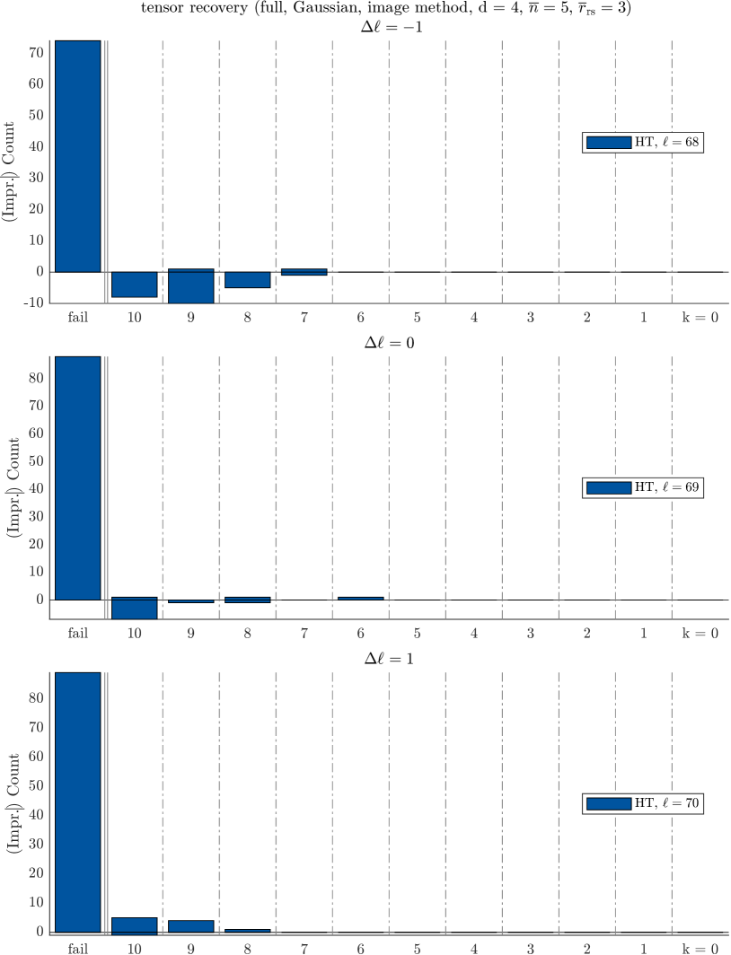
Figure SM1. Results for Experiment 7.1 as described in Appendix SM2.

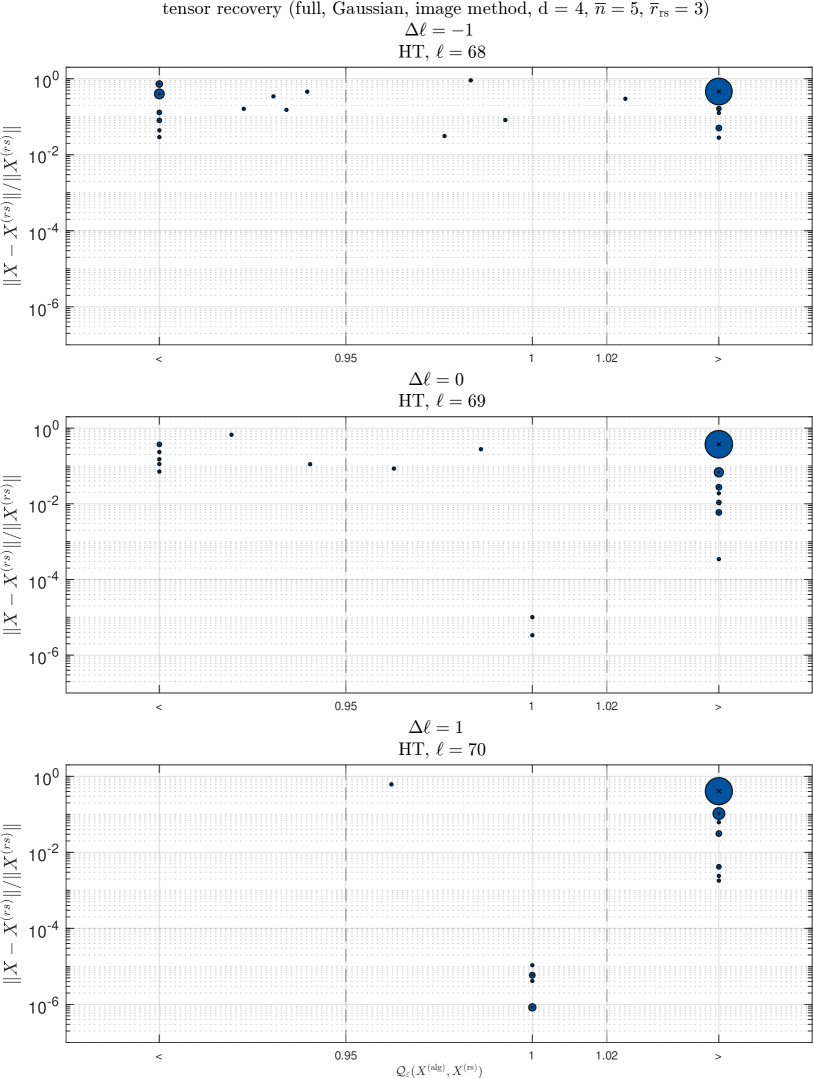
Figure SM2. Results for Experiment 7.1 as described in Appendix SM2.

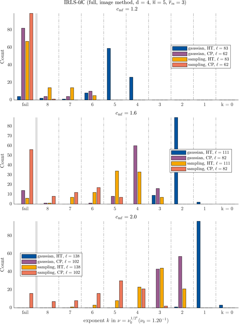
Figure SM3. Results for Experiment 7.2 as described in Appendix SM2.

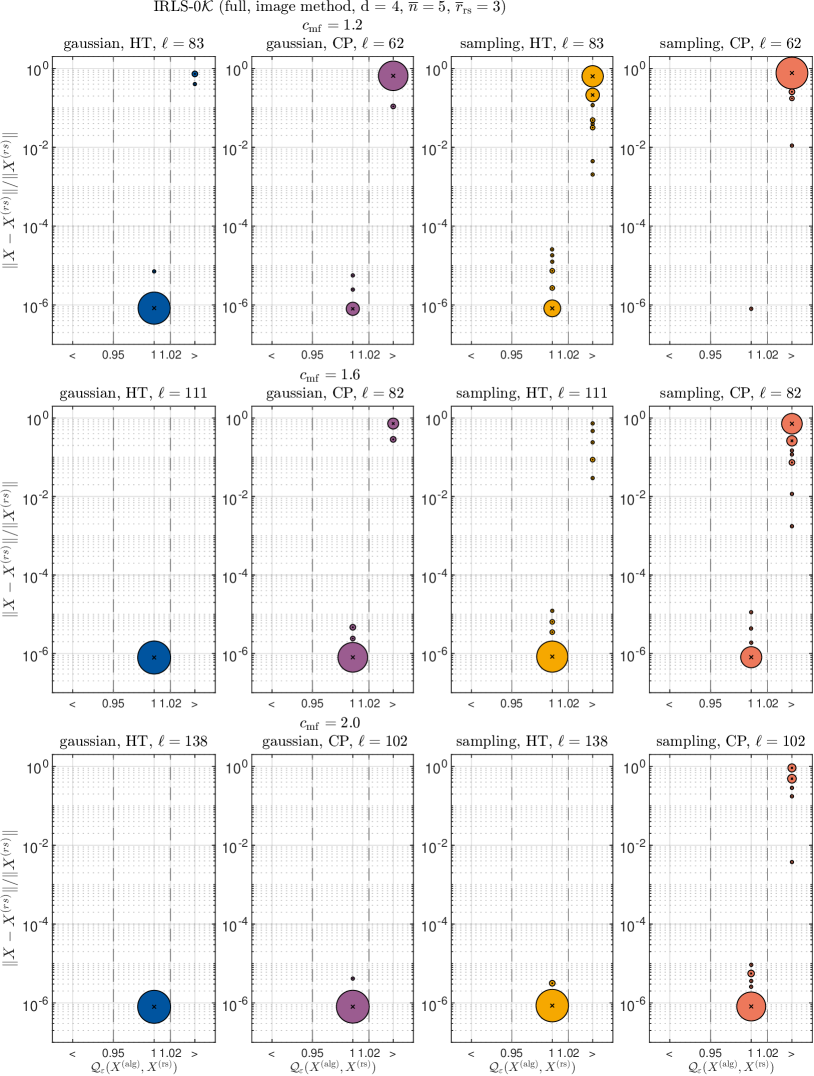
Figure SM4. Results for Experiment 7.2 as described in Appendix SM2.

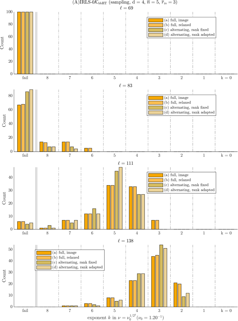
Figure SM5. Results for Experiment SM1 as described in Appendix SM2.

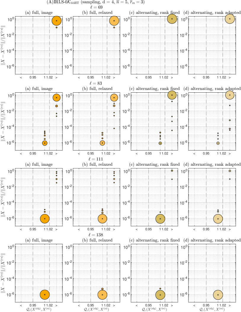
Figure SM6. Results for Experiment SM1 as described in Appendix SM2.

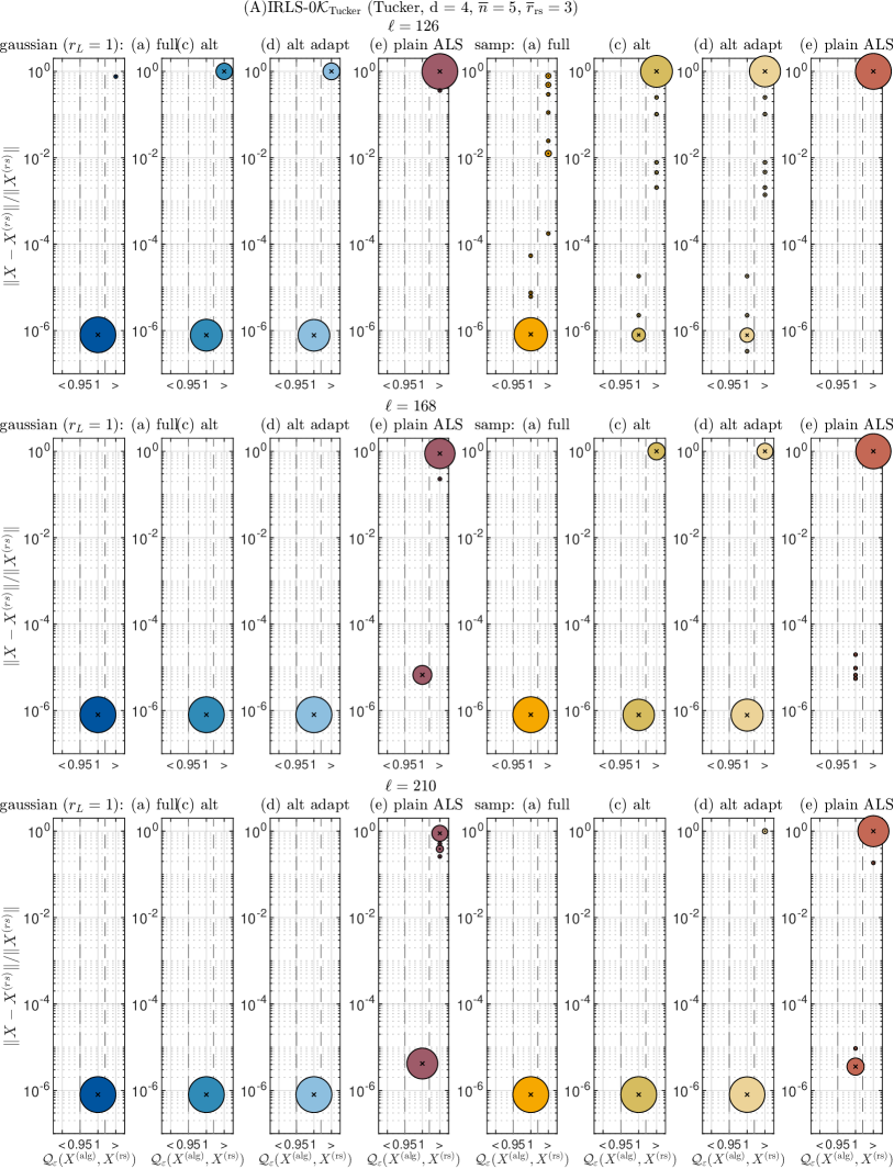
Figure SM7. Results for Experiment 7.3 as described in Appendix SM2.

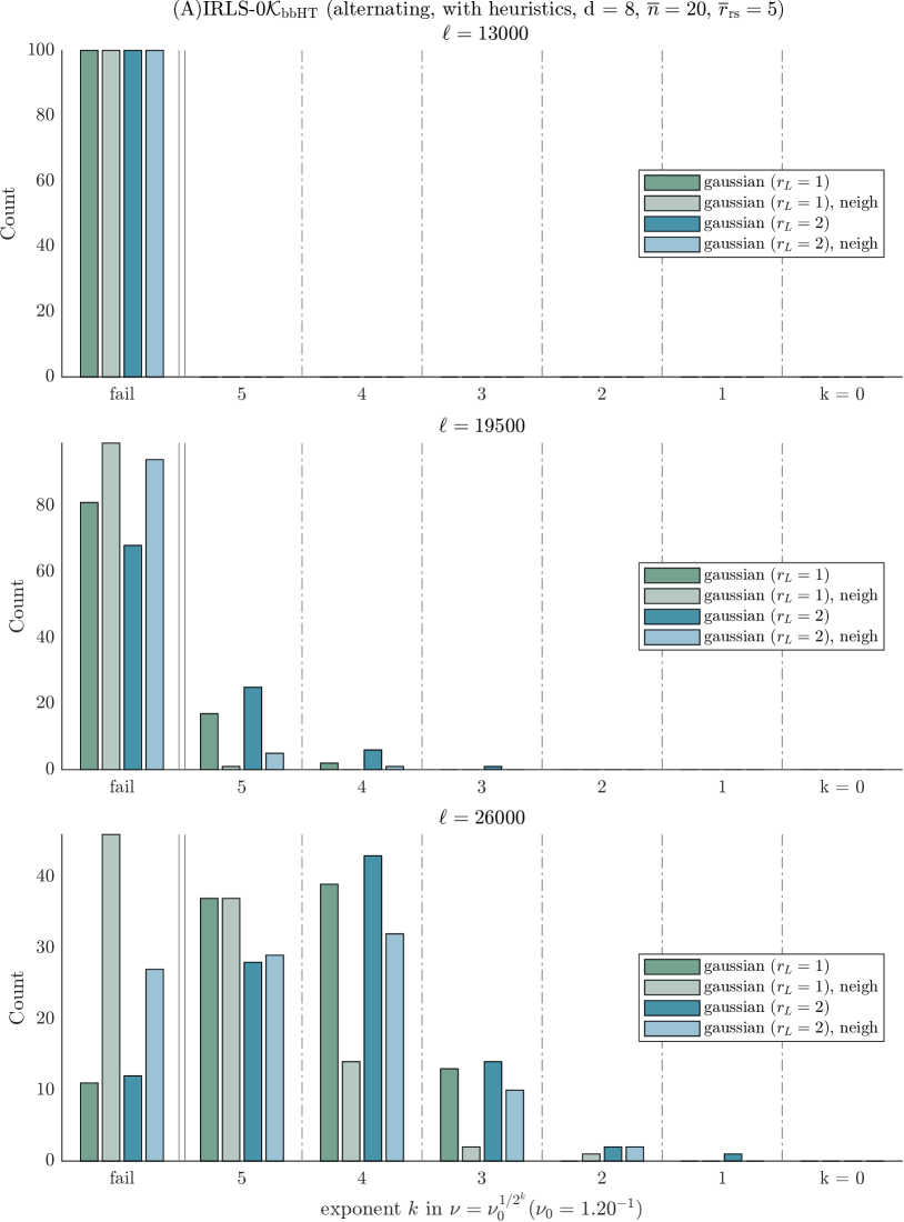
Figure SM8. Results for Experiment 7.4 as described in Appendix SM2.

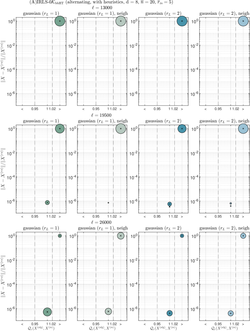
Figure SM9. Results for Experiment 7.4 as described in Appendix SM2.

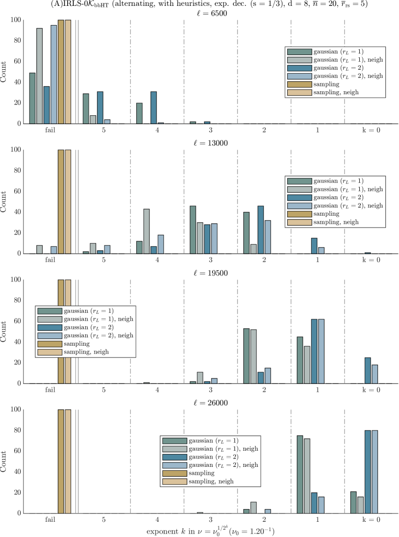
Figure SM10. Results for Experiment 7.4 as described in Appendix SM2.

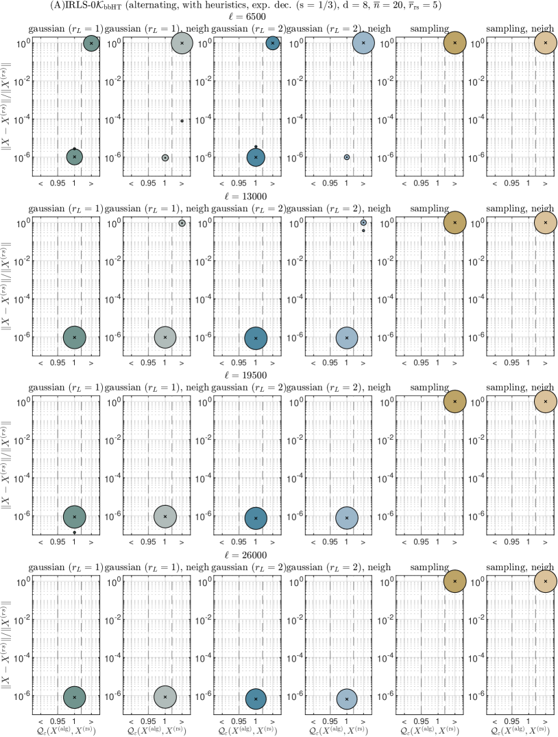
Figure SM11. Results for Experiment 7.4 as described in Appendix SM2.

Appendix SM4 Proof of Theorem 6.3

Following is the proof of Theorem 6.3 in minimally deviating notation. For the more elegant version, see Section SM5.2.

Proof.

Firstly, we consider a $|E_{Y}|+|E_{c}|$ dimensional tensor representation $G^{(\hat{J})}\in\mathbb{R}^{\bigtimes_{e\in E_{Y}}[n_{J_{e}}]}\otimes\mathfrak{H}_{\mathfrak{m}_{c}}$ of $\mathcal{N}_{\neq c}:\mathfrak{H}_{\mathfrak{m}_{c}}\rightarrow\mathbb{R}^{n_{1}\times\ldots\times n_{d}}$ and its adjoint. We can thus write

$$A^{({\hat{J}})}_{\alpha_{c}^{\prime},\{{\beta^{e}}^{\prime}\}_{e\in E_{c}};\,\alpha_{c},\{\beta^{e}\}_{e\in E_{c}}}\\ =\sum_{\alpha_{J_{e}}\,:\,e\in E_{Y}}G^{({\hat{J}})}_{\{\alpha_{J_{e}}\}_{e\in E_{Y}},\alpha_{c}^{\prime},\{{\beta^{e}}^{\prime}\}_{e\in E_{c}}}W^{({\hat{J}})}_{\alpha_{{\hat{J}}}^{\prime},\alpha_{{\hat{J}}}}G^{({\hat{J}})}_{\{\alpha_{J_{e}}\}_{e\in E_{Y}},\alpha_{c},\{\beta^{e}\}_{e\in E_{c}}}.$$

The representation $G^{(\hat{J})}$ can further be decomposed into a set of orthonormal matrices $Y^{(J_{e})}\in\mathbb{R}^{[n_{J_{e}}]\times[r^{(J_{e})}]}$, $e\in E_{Y}$, and the tensor $P^{(\hat{J})}\in\mathbb{R}^{\bigtimes_{v\in p}[n_{v}]\times\bigtimes_{{e}\in\partial{E}_{p}}[r^{(J_{e})}]}$ obtained via a contraction along the path $p$,

$$G^{({\hat{J}})}_{\{\alpha_{J_{e}}\}_{e\in E_{Y}},\alpha_{c},\{\beta^{e}\}_{e\in E_{c}}}=\sum_{\beta^{e}\,:\,{e}\in E_{Y}\setminus E_{c}}\prod_{e\in E_{Y}}Y^{(J_{e})}_{\alpha_{J_{e}},\beta^{e}}\ P^{(\hat{J})}_{\{\alpha_{v}\}_{v\in p},\{{\beta^{e}}\}_{e\in\partial{E}_{p}}}.$$

whereas the path evaluation is given by

$$P^{(\hat{J})}_{\{\alpha_{v}\}_{v\in p},\{{\beta^{e}}\}_{e\in\partial{E}_{p}}}=\tau_{r}(\{N_{v}\}_{v\in p})=\sum_{\beta^{{e}}\,:\,{e}\in\mathring{E}_{p}}\prod_{v\in p}(N_{v})_{\alpha_{v},\{{\beta^{e}}\}_{e\in E_{v}}}.$$

As Lemma 6.2 provides, we may replace $W^{({\hat{J}})}=W^{({\hat{J}})}_{\gamma,N,c}$. The matrices $Y^{(J)}$, $J\in\mathcal{K}^{\mathcal{S}_{c}}$, then cancel out due to orthonormality and we obtain 6.6 for

$$M^{(\hat{J})}_{{\beta^{e_{1}}}^{\prime},\beta^{e_{1}}}=\\ \sum_{\begin{array}[]{c}\scriptstyle{\beta^{e}}^{\prime},\beta^{e}\,:\,{e}\in E_{Y}\setminus E_{c},\\ \scriptstyle\alpha_{v}\,:\,v\in p\end{array}}\big{(}\prod_{e\in\partial{E}_{p}\setminus\{e_{1},\hat{e}\}}\delta_{{\beta^{e}}^{\prime},\beta^{e}}\big{)}P^{(\hat{J})}_{\{\alpha_{v}\}_{v\in p},\{{\beta^{e}}^{\prime}\}_{e\in\partial{E}_{p}}}H^{(\hat{J})}_{{\beta^{\hat{e}}}^{\prime},\beta^{\hat{e}}}P^{(\hat{J})}_{\{\alpha_{v}\}_{v\in p},\{{\beta^{e}}\}_{e\in\partial{E}_{p}}}$$

As the term $H^{(J)}$ can similarly be simplified, we have

$$H^{(\hat{J})}_{{\beta^{\hat{e}}}^{\prime},\beta^{\hat{e}}}=\sum_{\begin{array}[]{c}\scriptstyle{\beta^{e}}^{\prime},\beta^{e}\,:\,{e}\in E_{Y}\setminus\{\hat{e}\},\\ \scriptstyle\alpha_{v}\,:\,v\in p\end{array}}\big{(}\prod_{e\in E_{Y}\setminus\{\hat{e}\}}\delta_{{\beta^{e}}^{\prime},\beta^{e}}\big{)}P^{(+c,\hat{J})}_{\alpha_{p},\{{\beta^{e}}^{\prime}\}_{e\in E_{Y}}}P^{(+c,\hat{J})}_{\alpha_{p},\{\beta^{e}\}_{e\in E_{Y}}},$$

where

$$P^{(+c,\hat{J})}_{\alpha_{p},\{\beta^{e}\}_{e\in E_{Y}}}=\sum_{\beta^{e_{1}}}(N_{c})_{\alpha_{c},\{{\beta^{e}}\}_{e\in E_{c}}}P^{(\hat{J})}_{\{\alpha_{v}\}_{v\in p},\{{\beta^{e}}\}_{e\in\partial{E}_{p}}}.$$

By expanding and reordering the contractions within the path evaluations, we then arrive at 6.7 and 6.8. ∎

Appendix SM5 Tensor nodes

As indicated in Section 5.1, we in the following dismiss the indices in tensor contractions. What is here introduced as notation, is a simplified version of the formal arithmetic established in [25].

SM5.1. Self-emergent contractions

Though it is clear by Section 5, which tensors are assigned which labels, we here repeat this formal step. Such is indicated by writing $X=X(\{\alpha_{\mu}\}_{\mu\in[d]})\in\mathfrak{H}_{\{\alpha_{\mu}\}_{\mu\in[d]}}$ for any full tensor, or in case of its representation network $X=\tau_{r}(N)$, by

$$N=\{N_{v}\}_{v\in V},\quad N_{v}=N_{v}(\{\gamma\}_{\gamma\in\mathfrak{m}_{v}})\in\mathfrak{H}_{\mathfrak{m}_{v}}.$$

Avoiding the redundant notation such as in the expression 5.5, we simply write

$$X=\mathop{\boxtimes}_{v\in V}N_{v}.$$

The same symbol is used for any other contraction, such as in 5.6, translating to

$$\tau_{r}(\{N_{s}\}_{s\in S})_{\{\alpha_{s}\}_{s\in S}}=\mathop{\boxtimes}_{v\in S}N_{s}.$$

For any label $\gamma$, we denote the priorly used Kronecker deltas as formal objects $\Delta_{\gamma^{\prime},\gamma}\in\mathfrak{H}_{\{\gamma^{\prime},\gamma\}}$, or equivalently so for more than two labels. Instead of explicitly denoting primed labels, we instead define

$$(N_{v})_{\gamma\rightarrow\gamma^{\prime}}:=\Delta_{\gamma^{\prime},\gamma}\mathop{\boxtimes}N_{v},\quad\gamma\in\mathfrak{m}_{v}.$$

As shorthand notation, we further define $N_{v}^{\prime}=N_{v}^{\prime}(\alpha_{v},\{{\beta^{e}}^{\prime}\}_{e\in E_{v}})$ as

$$N_{v}^{\prime}:=(N_{v})_{\{{\beta^{e}}\}_{e\in E_{v}}\rightarrow\{{\beta^{e}}^{\prime}\}_{e\in E_{v}}}:=\big{(}\mathop{\boxtimes}_{e\in E_{v}}\Delta_{{\beta^{e}}^{\prime},\beta^{e}}\big{)}\mathop{\boxtimes}N_{v}.$$

For other tensors, the operator $(\cdot)^{\prime}$ likewise denotes a priming of all labels $\{\beta^{e}\}_{e\in E}$ assigned to such. The special case of an element-wise multiplication as in 6.4 is flagged via a superindex

$$L_{c}\boxtimes^{\zeta}L_{v}:=\Delta_{\zeta^{\prime\prime},\zeta^{\prime},\zeta}\boxtimes(\Delta_{\zeta^{\prime},\zeta}\boxtimes L_{c})\boxtimes(\Delta_{\zeta^{\prime\prime},\zeta}\boxtimes L_{v}).$$

We may thus equivalently write 6.4 as

$$\mathcal{L}(X)=L\mathop{\boxtimes}X\in\mathfrak{H}_{\zeta},\quad L=\rho_{r_{L}}(\{L_{v}\}_{v\in V})=\boxtimes^{\zeta}_{v\in V}L_{v}\in\mathfrak{H}_{\zeta\cup\{\alpha_{\mu}\}_{\mu\in[d]}}.$$

The expression 6.5 for instance takes the shorter shape $\mathcal{L}(X)=\mathop{\boxtimes}^{\zeta}_{v\in V}(L_{v}\mathop{\boxtimes}N_{v})$.

SM5.2. Alternative Theorems 6.3 and 6.4

While we may write $A^{(\hat{J})}=A^{(\hat{J})}(\alpha_{c}^{\prime},\{{\beta^{e}}^{\prime}\}_{e\in E_{c}},\alpha_{c},\{\beta^{e}\}_{e\in E_{c}})$, the identities in Theorem 6.3 become

(SM1) $$A^{({\hat{J}})}=\Delta_{\alpha_{c}^{\prime},\alpha_{c}}\mathop{\boxtimes}\big{(}\mathop{\boxtimes}_{e\in E_{c}\setminus\{e_{1}\}}\Delta_{{\beta^{e}}^{\prime},\beta^{e}}\big{)}\mathop{\boxtimes}M^{(\hat{J})},$$

for $M^{(\hat{J})}=M^{(\hat{J})}({\beta^{e_{1}}}^{\prime},\beta^{e_{1}})$ with

(SM2) $$M^{(\hat{J})} =\big{(}\mathop{\boxtimes}_{e\in\partial{E}_{p}\setminus\{e_{1},\hat{e}\}}\Delta_{{\beta^{e}}^{\prime},\beta^{e}}\big{)}\mathop{\boxtimes}\Big{(}\mathop{\boxtimes}_{v\in p}N_{v}^{\prime}\mathop{\boxtimes}N_{v}\Big{)}\mathop{\boxtimes}(H^{(\hat{J})}+\gamma I)^{-1},$$

as well as $H^{(\hat{J})}=H^{(\hat{J})}({\beta^{\hat{e}}}^{\prime},\beta^{\hat{e}})$ given by

(SM3) $$H^{(\hat{J})}=\big{(}\mathop{\boxtimes}_{e\in E_{Y}\setminus\{\hat{e}\}}\Delta_{{\beta^{e}}^{\prime},\beta^{e}}\big{)}\mathop{\boxtimes}_{v\in\{c\}\cup p}\Big{(}N_{v}^{\prime}\mathop{\boxtimes}N_{v}\Big{)}.$$

The identities appearing in the proof of Theorem 6.3, in turn, become

$$A^{({\hat{J}})}={G^{({\hat{J}})}}^{\prime}\mathop{\boxtimes}W^{({\hat{J}})}\mathop{\boxtimes}G^{({\hat{J}})},\quad G^{({\hat{J}})}=Y^{(J_{e})}\mathop{\boxtimes}P^{(\hat{J})},\quad P^{(\hat{J})}=\mathop{\boxtimes}_{v\in p}N_{v}$$

These tensors thereby have labels $G^{(\hat{J})}=G^{(\hat{J})}(\{\alpha_{J_{e}}\}_{e\in E_{Y}},\alpha_{c},\{\beta^{e}\}_{e\in E_{c}})$, as well as $Y^{(J_{e})}=Y^{(J_{e})}(\alpha_{J_{e}},\beta^{e})$, $e\in E_{Y}$, and $P^{(\hat{J})}=P^{(\hat{J})}(\{\alpha_{v}\}_{v\in p\cap[d]},\{\beta^{e}\}_{{e}\in\partial{E}_{p}})$. Further,

$$M^{(\hat{J})}=P^{(\hat{J})}_{\beta^{e_{1}}\rightarrow{\beta^{e_{1}}}^{\prime},\ \beta^{\hat{e}}\rightarrow{\beta^{\hat{e}}}^{\prime}}\mathop{\boxtimes}H^{(\hat{J})}\mathop{\boxtimes}P^{(\hat{J})}$$

and similarly

$$H^{(\hat{J})}=P^{(+c,\hat{J})}_{\beta^{\hat{e}}\rightarrow{\beta^{\hat{e}}}^{\prime}}\mathop{\boxtimes}P^{(+c,\hat{J})},\quad P^{(+c,\hat{J})}=N_{c}\mathop{\boxtimes}P^{(\hat{J})}$$

The identity in Corollary 6.4 on the other hand is simply $H^{(\hat{J})}=(N_{c})_{\beta^{\hat{e}}\rightarrow{\beta^{\hat{e}}}^{\prime}}\mathop{\boxtimes}N_{c}$.

SM5.3. Proofs of Propositions 6.5, 6.6 and 6.7

The recursion stated in Proposition 6.5 is

$$F_{c}=L_{c}\boxtimes^{\zeta}_{v\in\mathrm{neigh}(c)}S^{(J_{\{c,v\}})},$$

for $c\in V$ and

$$S^{(J_{\hat{e}})}=(L_{v}\mathop{\boxtimes}N_{v})\boxtimes_{b\in\mathrm{desc}_{c}(v)}^{\zeta}S^{(J_{\{v,b\}})},$$

with $\hat{e}=\{\mathrm{pred}_{c}(v),v\}$ for $v\in V\setminus\{c\}$.

Proof.

The recursion implies that $S^{(J_{\hat{e}})}=\mathop{\boxtimes}^{\zeta}_{h\in\mathrm{branch}_{c}(v)}(L_{h}\mathop{\boxtimes}N_{h})$. Thereby,

$$F_{c} :=L_{c}\mathop{\boxtimes}^{\zeta}_{v\in V\setminus\{c\}}(L_{v}\mathop{\boxtimes}N_{v})=L_{c}\mathop{\boxtimes}^{\zeta}_{v\in\mathrm{neigh}(c)}\mathop{\boxtimes}^{\zeta}_{h\in\mathrm{branch}_{c}(v)}(L_{h}\mathop{\boxtimes}N_{h})$$

provides the to be shown, first identity. ∎

The recursion in Proposition 6.6 is

$$\sum_{\hat{J}\in\mathcal{K}}A^{({\hat{J}})}=\Delta_{\alpha_{c}^{\prime},\alpha_{c}}\mathop{\boxtimes}\sum_{v\in\mathrm{neigh}(c)}\big{(}\mathop{\boxtimes}_{e\in E_{c}\setminus\{\{c,v\}\}}\Delta_{{\beta^{e}}^{\prime},\beta^{e}}\big{)}\mathop{\boxtimes}B^{(J_{\{c,v\}})},$$

where for $\hat{e}=\{p_{-1},v\}$, $p_{-1}=\mathrm{pred}_{c}(v)$, $v\in V\setminus\{c\}$, it is

$$\widetilde{B}^{(J_{\{v,b\}})}=(N_{v})_{\beta^{\hat{e}}\rightarrow{\beta^{\hat{e}}}^{\prime},\ \beta^{\{v,b\}}\rightarrow{\beta^{\{v,b\}}}^{\prime}}\mathop{\boxtimes}B^{(J_{\{v,b\}})}\mathop{\boxtimes}N_{v},$$

for $b\in\mathrm{desc}_{c}(v)$.

Proof.

By definition,

$$\sum_{\hat{J}\in\mathcal{K}}A^{({\hat{J}})} =\sum_{v\in V\setminus\{c\}}\Delta_{\alpha_{c}^{\prime},\alpha_{c}}\mathop{\boxtimes}\big{(}\mathop{\boxtimes}_{e\in E_{c}\setminus\{\{c,p_{1}(v)\}\}}\Delta_{{\beta^{e}}^{\prime},\beta^{e}}\big{)}\mathop{\boxtimes}M^{(J_{\{\mathrm{pred}_{c}(v),v\}})}$$

$$=\Delta_{\alpha_{c}^{\prime},\alpha_{c}}\mathop{\boxtimes}\sum_{v\in\mathrm{neigh}(c)}\big{(}\mathop{\boxtimes}_{e\in E_{c}\setminus\{\{c,v\}\}}\Delta_{{\beta^{e}}^{\prime},\beta^{e}}\big{)}\mathop{\boxtimes}\sum_{b\in\mathrm{branch}_{c}(v)}M^{(J_{\{\mathrm{pred}_{c}(b),b\}})}.$$

Let each be $p=(c,h)$, with $e_{1}=\{c,p_{1}\}$, $\hat{e}=\{p_{-1},h\}$, for $h\in V\setminus\{c\}$. We show that

$$\sum_{b\in\mathrm{branch}_{c}(h)}M^{(J_{\{\mathrm{pred}_{c}(b),b\}})} =\big{(}\mathop{\boxtimes}_{e\in\partial{E}_{p}\setminus\{e_{1},\hat{e}\}}\Delta_{{\beta^{e}}^{\prime},\beta^{e}}\big{)}\mathop{\boxtimes}\Big{(}\mathop{\boxtimes}_{v\in{p}}N_{v}^{\prime}\mathop{\boxtimes}N_{v}\Big{)}\mathop{\boxtimes}B^{(J_{\hat{e}})}$$

by induction over the cardinality of $\mathrm{branch}_{c}(h)$. The induction start for a cardinality of $1$ is then given by SM2 and the definition of $B^{(J)}$. In turn, given the tree structure of $G$ and the induction hypothesis, it follows that

$$\ \sum_{b\in\mathrm{branch}_{c}(h)}M^{(J_{\{\mathrm{pred}_{c}(b),b\}})}=M^{(J_{\hat{e}})}+\sum_{b\in\mathrm{desc}_{c}(h)}\sum_{w\in\mathrm{branch}_{c}(b)}M^{(J_{\{\mathrm{pred}_{c}(w),w\}})}$$

$$= \ \big{(}\mathop{\boxtimes}_{e\in\partial{E}_{p}\setminus\{e_{1},\hat{e}\}}\Delta_{{\beta^{e}}^{\prime},\beta^{e}}\big{)}\mathop{\boxtimes}\Big{(}\mathop{\boxtimes}_{v\in{p}}N_{v}^{\prime}\mathop{\boxtimes}N_{v}\Big{)}\mathop{\boxtimes}(H^{(J_{\hat{e}})}+\gamma I)^{-1}$$

$$+ \ \sum_{b\in\mathrm{desc}_{c}(h)}\big{(}\mathop{\boxtimes}_{e\in\partial{E}_{(c,b)}\setminus\{e_{1},\{h,b\}\}}\Delta_{{\beta^{e}}^{\prime},\beta^{e}}\big{)}\mathop{\boxtimes}\Big{(}\mathop{\boxtimes}_{v\in{(c,b)}}N_{v}^{\prime}\mathop{\boxtimes}N_{v}\Big{)}\mathop{\boxtimes}B^{(J_{\{h,b\}})}$$

$$= \ \big{(}\mathop{\boxtimes}_{e\in\partial{E}_{p}\setminus\{e_{1},\hat{e}\}}\Delta_{{\beta^{e}}^{\prime},\beta^{e}}\big{)}\mathop{\boxtimes}\Big{(}\mathop{\boxtimes}_{v\in{p}}N_{v}^{\prime}\mathop{\boxtimes}N_{v}\Big{)}\mathop{\boxtimes}\Big{(}(H^{(J_{\hat{e}})}+\gamma I)^{-1}$$

$$+ \ \sum_{b\in\mathrm{desc}_{c}(h)}\big{(}\mathop{\boxtimes}_{e\in E_{h}\setminus\{\hat{e},\{h,b\}\}}\Delta_{{\beta^{e}}^{\prime},\beta^{e}}\big{)}\mathop{\boxtimes}N_{h}^{\prime}\mathop{\boxtimes}B^{(J_{\{h,b\}})}\mathop{\boxtimes}N_{h}\Big{)}$$

$$= \ \big{(}\mathop{\boxtimes}_{e\in\partial{E}_{p}\setminus\{e_{1},\hat{e}\}}\Delta_{{\beta^{e}}^{\prime},\beta^{e}}\big{)}\mathop{\boxtimes}\Big{(}\mathop{\boxtimes}_{v\in{p}}N_{v}^{\prime}\mathop{\boxtimes}N_{v}\Big{)}\mathop{\boxtimes}\Big{(}(H^{(J_{\hat{e}})}+\gamma I)^{-1}$$

$$+ \ \sum_{b\in\mathrm{desc}_{c}(h)}(N_{h})_{\beta^{\hat{e}}\rightarrow{\beta^{\hat{e}}}^{\prime},\ \beta^{\{h,b\}}\rightarrow{\beta^{\{h,b\}}}^{\prime}}\mathop{\boxtimes}B^{(J_{\{h,b\}})}\mathop{\boxtimes}N_{h}\Big{)}.$$

The last to be shown step follows as by definition

$$B^{(J_{\hat{e}})}=(H^{(J_{\hat{e}})}+\gamma I)^{-1}+\sum_{b\in\mathrm{desc}_{c}(h)}(N_{h})_{\beta^{\hat{e}}\rightarrow{\beta^{\hat{e}}}^{\prime},\ \beta^{\{h,b\}}\rightarrow{\beta^{\{h,b\}}}^{\prime}}\mathop{\boxtimes}B^{(J_{\{h,b\}})}\mathop{\boxtimes}N_{h}.$$

∎

The recursion in Proposition 6.7, for $\hat{e}=\{p_{-1},v\}$, $p_{-1}=\mathrm{pred}_{c}(v)$, $v\in V\setminus\{c\}$, is

$$H^{(J_{\{v,b\}})}=(N_{v})_{\beta^{\{v,b\}}\rightarrow{\beta^{\{v,b\}}}^{\prime},\ \beta^{\hat{e}}\rightarrow{\beta^{\hat{e}}}^{\prime}}\mathop{\boxtimes}H^{(J_{\hat{e}})}\mathop{\boxtimes}N_{v},$$

for $b\in\mathrm{desc}_{c}(v)$.

Proof.

Using the identity SM3 on both sides, we obtain

$$\ (N_{v})_{\beta^{\{v,b\}}\rightarrow{\beta^{\{v,b\}}}^{\prime},\ \beta^{\hat{e}}\rightarrow{\beta^{\hat{e}}}^{\prime}}\mathop{\boxtimes}H^{(J_{\hat{e}})}\mathop{\boxtimes}N_{v}$$

$$= \ (N_{v})_{\beta^{\{v,b\}}\rightarrow{\beta^{\{v,b\}}}^{\prime},\ \beta^{\hat{e}}\rightarrow{\beta^{\hat{e}}}^{\prime}}\mathop{\boxtimes}\big{(}\mathop{\boxtimes}_{e\in\partial{E}_{\{c\}\cup p}\setminus\{\hat{e}\}}\Delta_{{\beta^{e}}^{\prime},\beta^{e}}\big{)}\mathop{\boxtimes}_{w\in\{c\}\cup p}\Big{(}N_{w}^{\prime}\mathop{\boxtimes}N_{w}\Big{)}\mathop{\boxtimes}N_{v}$$

$$= \ \big{(}\mathop{\boxtimes}_{e\in E_{v}\setminus\{\hat{e},\{v,b\}\}}\Delta_{{\beta^{e}}^{\prime},\beta^{e}}\big{)}\mathop{\boxtimes}N_{v}^{\prime}\mathop{\boxtimes}\big{(}\mathop{\boxtimes}_{e\in\partial{E}_{\{c\}\cup p}\setminus\{\hat{e}\}}\Delta_{{\beta^{e}}^{\prime},\beta^{e}}\big{)}\mathop{\boxtimes}_{w\in\{c\}\cup p}\Big{(}N_{w}^{\prime}\mathop{\boxtimes}N_{w}\Big{)}\mathop{\boxtimes}N_{v}$$

$$= \ \big{(}\mathop{\boxtimes}_{e\in\partial{E}_{\{c\}\cup(c,b)}\setminus\{\{v,b\}\}}\Delta_{{\beta^{e}}^{\prime},\beta^{e}}\big{)}\mathop{\boxtimes}_{w\in\{c\}\cup(c,b)}\Big{(}N_{w}^{\prime}\mathop{\boxtimes}N_{w}\Big{)}=H^{(J_{\{v,b\}})},$$

which was to be shown. ∎

SM5.4. Detailed AIRLS-$0K$ algorithm

Section SM5.4 summarizes the AIRLS-$0\mathcal{K}$ method as covered in Section 6. In our experiments, we have chosen the therein appearing constant as $c_{\mathcal{L}}=\frac{1}{4}|\mathcal{K}|^{-1}\|L\|_{F}^{2}/n_{[d]}$. The heuristics laid out in Appendix SM6 are marked as possibly applicable statements.

  Algorithm 3 Detailed AIRLS-$0\mathcal{K}$ method

 

1:  derive tree $G=(V,E)$ from $\mathcal{K}$

2:  set $N=\{N\}_{v\in V}\in\mathcal{D}_{r}$, $\gamma^{(0)}>0$, $c_{0}\in V$

3:  possibly introduce validation set (cf. Section SM6.1)

3:  

3:   // let $J_{e}\in\mathcal{K}^{\mathcal{S}_{c_{0}}}$, $e\in E$

3:   // orthonormalize $\{N_{v}\}_{v\in V}$ with respect to $c_{0}$ (cf. Theorem 5.11) and initialize the branch evaluations $\{S^{(J_{e})}\}_{e\in E}$ (cf. Proposition 6.5)

4:  $\widetilde{V}:=\mathrm{leaves}(c_{0})$

5:  while $\widetilde{V}\neq\{c_{0}\}$  do

6:     for $v\in\widetilde{V}\setminus\{c_{0}\}$ do

7:        $p_{-1}:=\mathrm{pred}_{c_{0}}(v)$, $\hat{e}:=\{p_{-1},v\}$

8:        $QR:=N_{v}^{[\mathfrak{m}_{v}\setminus\{\beta^{\hat{e}}\}]}$, $N_{v}^{[\mathfrak{m}_{v}\setminus\{\beta^{\hat{e}}\}]}:=Q$, $N_{p_{-1}}^{[\beta^{\hat{e}}]}:=RN_{p_{-1}}^{[\beta^{\hat{e}}]}$

9:        $S^{(J_{\hat{e}})}:=(L_{v}\boxtimes N_{v})\boxtimes^{\zeta}_{h\in\mathrm{desc}_{c_{0}}(v)}S^{(J_{\{v,h\}})}$

10:     end for

11:     $\widetilde{V}:=\bigcup_{v\in\widetilde{V}}\mathrm{pred}_{c_{0}}(v)$

12:  end while

12:  

12:   // implicitly declare iterate $X^{(0)}=\tau_{r}(\{N_{v}\}_{v\in V})$

13:  for $i=1,2,\ldots$ do

13:      // calculate $\{H^{(i-1,J)}\}_{J\in\mathcal{K}^{\mathcal{S}_{c_{i-1}}}}$ (cf. Propositions 6.7 and 6.4) or possibly limit set via maximal distance of ${\widetilde{v}}\in\widetilde{V}$ to $c_{i-1}$:

14:     for $v\in\mathrm{neigh}(c_{i-1})$ do

15:        $\hat{e}:=\{c_{i-1},v\}$

16:        $H^{(J_{\hat{e}})}:=(N_{c_{i-1}})_{\beta^{\hat{e}}\rightarrow{\beta^{\hat{e}}}^{\prime}}\mathop{\boxtimes}N_{c_{i-1}}$

17:     end for

18:     $\widetilde{V}:=\bigcup_{v\in\mathrm{neigh}(c_{i-1})}\mathrm{desc}_{c_{i-1}}(v)$

19:     while $\widetilde{V}\neq\mathrm{leaves}(c_{0})$  do

20:        for ${\widetilde{v}}\in\widetilde{V}\setminus\mathrm{lea{\widetilde{v}}es}(c_{0})$ do

21:           $p_{-1}:=\mathrm{pred}_{c_{0}}({\widetilde{v}})$, $\hat{e}:=\{p_{-1},{\widetilde{v}}\}$

22:           for $b\in\mathrm{desc}_{c_{i-1}}({\widetilde{v}})$ do

23:              $H^{(J_{\{{\widetilde{v}},b\}})}:=(N_{\widetilde{v}})_{\beta^{\{{\widetilde{v}},b\}}\rightarrow{\beta^{\{{\widetilde{v}},b\}}}^{\prime},\beta^{\hat{e}}\rightarrow{\beta^{\hat{e}}}^{\prime}}\mathop{\boxtimes}H^{(J_{\hat{e}})}\mathop{\boxtimes}N_{{\widetilde{v}}}$

24:           end for

25:        end for

26:        $\widetilde{V}:=\bigcup_{{\widetilde{v}}\in\widetilde{V}}\mathrm{desc}_{c_{i-1}}({\widetilde{v}})$

27:     end while

27:     

27:      // calculate $\{B^{(i-1,J)}\}_{J\in\mathcal{K}^{\mathcal{S}_{c_{i-1}}}}$ (cf. Proposition 6.6) or possibly limit set via maximal distance of ${\widetilde{v}}\in\widetilde{V}$ to $c_{i-1}$:

28:     $\widetilde{V}:=\mathrm{leaves}(c_{0})$

29:     while $\widetilde{V}\neq\{c_{0}\}$  do

30:        for ${\widetilde{v}}\in\widetilde{V}\setminus\{c_{0}\}$ do

31:           $p_{-1}:=\mathrm{pred}_{c_{0}}({\widetilde{v}})$, $\hat{e}:=\{p_{-1},{\widetilde{v}}\}$

32:           for $b\in\mathrm{desc}_{c_{i-1}}({\widetilde{v}})$ do

33:              $\widetilde{B}^{(i-1,J_{\{{\widetilde{v}},b\}})}:=(N_{h})_{\beta^{\hat{e}}\rightarrow{\beta^{\hat{e}}}^{\prime},\beta^{\{{\widetilde{v}},b\}}\rightarrow{\beta^{\{{\widetilde{v}},b\}}}^{\prime}}\mathop{\boxtimes}B^{(i-1,J_{\{{\widetilde{v}},b\}})}\mathop{\boxtimes}\mathbb{N}{\widetilde{v}}tensor{{\widetilde{v}}}$

34:           end for

35:           $B^{(i-1,J_{\hat{e}})}:=(H^{(i-1,J_{\hat{e}})}+\gamma^{(i-1)}I)^{-1}+\sum_{b\in\mathrm{desc}_{c_{i-1}}({\widetilde{v}})}\widetilde{B}^{(J_{\{{\widetilde{v}},b\}})}$

36:        end for

37:        $\widetilde{V}:=\bigcup_{{\widetilde{v}}\in\widetilde{V}}\mathrm{pred}_{c_{0}}({\widetilde{v}})$

38:     end while

38:     

38:      // solve and update representation (cf. 6.3, 6.6 and 6.5) possibly using iterative solver (cf. Section SM6.5)

39:     $A^{(i-1)}:=\Delta_{\alpha_{c}^{\prime},\alpha_{c}}\mathop{\boxtimes}\sum_{v\in\mathrm{neigh}({c_{i-1}})}\big{(}\mathop{\boxtimes}_{e\in E_{c_{i-1}}\setminus\{\{{c_{i-1}},v\}\}}\Delta_{{\beta^{e}}^{\prime},\beta^{e}}\big{)}\mathop{\boxtimes}B^{(J_{{\{{c_{i-1}},v\}}})}$

40:     $F^{(i-1)}:=L_{c_{i-1}}\boxtimes^{\zeta}_{v\in\mathrm{neigh}(c_{i-1})}S^{(J_{\{c_{i-1},v\}})}$

41:     solve $(F^{(i-1)}_{\mathfrak{m}_{c_{i-1}}\rightarrow\mathfrak{m}_{c_{i-1}}^{\prime}}\boxtimes F^{(i-1)}+c_{\mathcal{L}}\gamma^{(i-1)}A^{(i-1)})\boxtimes N^{+}_{c_{i-1}}=F^{(i-1)}_{\mathfrak{m}_{c_{i-1}}\rightarrow\mathfrak{m}_{c_{i-1}}^{\prime}}\boxtimes y$

42:     $N_{c_{i-1}}:=N_{c_{i-1}}^{+}$

42:     

42:      // let $J_{e}\in\mathcal{K}^{\mathcal{S}_{c_{i}}}$, $e\in E$, and shift root:

43:     set $c_{i}\in V\setminus\{c_{i-1}\}$ (cf. Section 6.1)

43:     

43:      // orthonormalize $\{N_{v}\}_{v\in V}$ with respect to $c_{i}$ (cf. Theorem 5.11) and supplement the missing branch evaluations of $\{S^{(J_{e})}\}_{e\in E}$ (cf. Proposition 6.5)

44:     set $p$ as path from including $c_{i-1}$ to including $c_{i}$ (cf. Section 5.2)

45:     for $j=2,\ldots,|p|$ do

46:        $\hat{e}:=\{p_{j-1},p_{j}\}$

47:        $U\operatorname{diag}(\sigma^{(J_{\hat{e}})})V^{T}:=N_{p_{j-1}}^{[\mathfrak{m}_{p_{j-1}}\setminus\{\beta^{\hat{e}}\}]}$

48:        possibly adapt rank $r\in\mathbb{N}^{\mathcal{K}}$ via according modification of the SVD components $U$, $\operatorname{diag}(\sigma^{(J_{\hat{e}})})$ and $V^{T}$ (cf. Section SM6.3)

49:        $N_{p_{j-1}}^{[\mathfrak{m}_{p_{j-1}}\setminus\{\beta^{\hat{e}}\}]}:=U\operatorname{diag}(\sigma^{(J_{\hat{e}})})$, $N_{p_{j}}^{[\beta^{\hat{e}}]}:=V^{T}N_{p_{j}}^{[\beta^{\hat{e}}]}$

50:        $S^{(J_{\hat{e}})}:=(L_{p_{j-1}}\boxtimes N_{p_{j-1}})\boxtimes^{\zeta}_{h\in\mathrm{desc}_{c_{i}}({p_{j-1}})}S^{(J_{\{{p_{j-1}},h\}})}$

51:     end for

51:     

51:      // implicitly declare iterate $X^{(i)}=\tau_{r}(\{N_{v}\}_{v\in V})$

52:     set $\gamma^{(i)}\leq\gamma^{(i-1)}$ (possibly bound from above, cf. Section SM6.2)

53:     consider break possibly also based on validation residual

54:  end for

55:  possibly repeat as post-iteration with adapted parameters to appropriately truncate representation (cf. Section SM6.4)

 

Appendix SM6 Practical and Heuristic Aspects

In Experiment 7.4, the AIRLS-$0\mathcal{K}$ algorithm is enhanced through the use of the following heuristics as embedded in Section SM5.4.

SM6.1. Validation set

A fraction of measurements is passively used to instead validate the progress allowing for more suitable breaking criteria and to adaptively control the parameter $\gamma$ (cf. Section SM6.2). This however assumes that the algorithm despite the decreased number of actively used measurements still converges to the essentially same solution.

SM6.2. Adaptive decay of regularization parameter $\gamma$

Practice shows that, additionally to the constant decline, carefully bounding $\gamma$ from above by a value proportional to the residual norm on the validation measurements (cf. Section SM6.1) can speed up convergence considerably without infringing upon the approximation.

SM6.3. Explicit rank adaption

The AIRLS-$0\mathcal{K}$ algorithm necessarily relies on the choice of some $\{r^{(J)}\}_{J\in\mathcal{K}}$ which bounds the ranks of the iterate. An adaptive determination can save a considerable amount of computational complexity. Introducing or removing a singular value $\sigma^{(J)}_{r^{(J)}}(X)$ (thus changing the rank of the iterate), that is small compared to $\gamma$, only marginally influences the iteration. A method that has proven itself reliable in practice is to adapt each single rank $r^{(J)}$, $J\in\mathcal{K}$, such that always $\sigma^{(J)}_{r^{(J)}-2}(X)>\frac{1}{2}\sqrt{\gamma}$, but $\sigma^{(J)}_{r^{(J)}-1}(X)<\frac{1}{2}\sqrt{\gamma}$. Thereby, there are always exactly two comparatively low singular values with respect to each subset $J$.

SM6.4. AIRLS-$0\mathcal{K}$ internal post-iteration

In particular if the ranks are explicitly adapted, some singular values of the final iterate may be small enough such that a truncation of such seems more reasonable. Instead of a separate procedure that does not consider the original problem setting, a better approximation can be achieved by letting the algorithm proceed some additional iterations but with adapted meta parameters and for a specifically chosen value $\gamma$. Alternatively for small dimensions, the post-iteration scheme as discussed in Section 7.4 may be utilized.

SM6.5. Solving linear subsystems with iterative solvers

The linear subproblems that appear in each optimization step might become too large to solve explicitely using ordinary, full matrix vector calculus. Iterative solvers, such as preconditioned CG, can be applied to reduce the order of complexity significantly by exploiting the given low rank as well as additive structures. Whether this is truly beneficial naturally depends on the exact sizes that are involved, and not least the implementation.

References

- [1] J. Ballani, L. Grasedyck, and M. Kluge, Black box approximation of tensors in hierarchical tucker format, Linear Algebra and its Applications, 438 (2013), pp. 639 – 657.
- [2] C. Bayer, M. Eigel, L. Sallandt, and P. Trunschke, Pricing high-dimensional bermudan options with hierarchical tensor formats, 2021.
- [3] P. Breiding, T. O. Çelik, T. Duff, A. Heaton, A. Maraj, A.-L. Sattelberger, L. Venturello, and O. Yürük, Nonlinear algebra and applications, 2021.
- [4] P. Breiding, F. Gesmundo, M. Michałek, and N. Vannieuwenhoven, Algebraic compressed sensing (in preparation). 2021.
- [5] E. J. Candès, M. B. Wakin, and S. P. Boyd, Enhancing sparsity by reweighted l1 minimization, Journal of Fourier Analysis and Applications, 14 (2008), pp. 877–905.
- [6] L. Chiantini, G. Ottaviani, and N. Vannieuwenhoven, An algorithm for generic and low-rank specific identifiability of complex tensors, SIAM Journal on Matrix Analysis and Applications, 35 (2014), pp. 1265–1287.
- [7] I. Daubechies, R. DeVore, M. Fornasier, and C. S. Güntürk, Iteratively reweighted least squares minimization for sparse recovery, Communications on Pure and Applied Mathematics, 63 (2010), pp. 1–38.
- [8] L. De Lathauwer, A survey of tensor methods, in 2009 IEEE International Symposium on Circuits and Systems (ISCAS), May 2009, pp. 2773–2776.
- [9] L. De Lathauwer, B. De Moor, and J. Vandewalle, A multilinear singular value decomposition, SIAM Journal on Matrix Analysis and Applications, 21 (2000), pp. 1253–1278.
- [10] A. Falcó, W. Hackbusch, and A. Nouy, Tree-based tensor formats, SeMA Journal, (2018).
- [11] M. Fornasier, H. Rauhut, and R. Ward, Low-rank matrix recovery via iteratively reweighted least squares minimization, SIAM Journal on Optimization, 21 (2011), pp. 1614–1640.
- [12] S. Gandy, B. Recht, and I. Yamada, Tensor completion and low-n-rank tensor recovery via convex optimization, Inverse Problems, 27 (2011), p. 025010.
- [13] A. Goeßmann, M. Götte, I. Roth, R. Sweke, G. Kutyniok, and J. Eisert, Tensor network approaches for learning non-linear dynamical laws, 2020.
- [14] M. Götte, R. Schneider, and P. Trunschke, A block-sparse tensor train format for sample-efficient high-dimensional polynomial regression, 2021.
- [15] L. Grasedyck, Hierarchical singular value decomposition of tensors, SIAM Journal on Matrix Analysis and Applications, 31 (2010), pp. 2029–2054.
- [16] L. Grasedyck and S. Krämer, Stable als approximation in the tt-format for rank-adaptive tensor completion, Numerische Mathematik, (2019).
- [17] L. Grasedyck, D. Kressner, and C. Tobler, A literature survey of low-rank tensor approximation techniques, GAMM-Mitteilungen, 36 (2013), pp. 53–78.
- [18] E. Grelier, A. Nouy, and M. Chevreuil, Learning with tree-based tensor formats, 2019.
- [19] C. Haberstich, A. Nouy, and G. Perrin, Active learning of tree tensor networks using optimal least-squares, 2021.
- [20] S. Holtz, T. Rohwedder, and R. Schneider, The alternating linear scheme for tensor optimization in the tensor train format, SIAM Journal on Scientific Computing, 34 (2012), pp. A683–A713.
- [21] S. Holtz, T. Rohwedder, and R. Schneider, On manifolds of tensors of fixed tt-rank, Numerische Mathematik, 120 (2012), pp. 701–731.
- [22] Y. Kapushev, I. Oseledets, and E. Burnaev, Tensor completion via gaussian process–based initialization, SIAM Journal on Scientific Computing, 42 (2020), pp. A3812–A3824.
- [23] T. G. Kolda and B. W. Bader, Tensor decompositions and applications, SIAM Review, 51 (2009), pp. 455–500.
- [24] S. Krämer, A geometric description of feasible singular values in the tensor train format, SIAM Journal on Matrix Analysis and Applications, 40 (2019), pp. 1153–1178.
- [25] S. Krämer, Tree tensor networks, associated singular values and high-dimensional approximation, dissertation, RWTH Aachen University, Aachen, 2020. Veröffentlicht auf dem Publikationsserver der RWTH Aachen University; Dissertation, RWTH Aachen University, 2020.
- [26] S. Krämer, Asymptotic log-det rank minimization via (alternating) iteratively reweighted least squares, 2021.
- [27] D. Kressner, M. Steinlechner, and B. Vandereycken, Low-rank tensor completion by riemannian optimization, BIT Numerical Mathematics, 54 (2014), pp. 447–468.
- [28] Y. Liu and F. Shang, An efficient matrix factorization method for tensor completion, IEEE Signal Processing Letters, 20 (2013), pp. 307–310.
- [29] K. Mohan and M. Fazel, Iterative reweighted algorithms for matrix rank minimization, Journal of Machine Learning Research, 13 (2012), pp. 3441–3473.
- [30] A. Nouy, Low-Rank Tensor Methods for Model Order Reduction, Springer International Publishing, Cham, 2017, pp. 857–882.
- [31] I. Oseledets and E. Tyrtyshnikov, Tt-cross approximation for multidimensional arrays, Linear Algebra and its Applications, 432 (2010), pp. 70 – 88.
- [32] I. V. Oseledets, Tensor-train decomposition, SIAM Journal on Scientific Computing, 33 (2011), pp. 2295–2317.
- [33] Y. Qi, P. Comon, and L.-H. Lim, Semialgebraic geometry of nonnegative tensor rank, SIAM Journal on Matrix Analysis and Applications, 37 (2016), pp. 1556–1580.
- [34] H. Rauhut, R. Schneider, and Ž. Stojanac, Tensor Completion in Hierarchical Tensor Representations, Springer International Publishing, Cham, 2015, pp. 419–450.
- [35] M. Signoretto, Q. Tran Dinh, L. De Lathauwer, and J. A. K. Suykens, Learning with tensors: a framework based on convex optimization and spectral regularization, Machine Learning, 94 (2014), pp. 303–351.
- [36] C. D. Silva and F. J. Herrmann, Optimization on the hierarchical tucker manifold – applications to tensor completion, Linear Algebra and its Applications, 481 (2015), pp. 131 – 173.
- [37] M. Sørensen and L. De Lathauwer, Fiber sampling approach to canonical polyadic decomposition and application to tensor completion, SIAM Journal on Matrix Analysis and Applications, 40 (2019), pp. 888–917.
- [38] M. Sørensen, N. D. Sidiropoulos, and L. De Lathauwer, Canonical polyadic decomposition of a tensor that has missing fibers: A monomial factorization approach, in ICASSP 2019 - 2019 IEEE International Conference on Acoustics, Speech and Signal Processing (ICASSP), May 2019, pp. 7490–7494.
- [39] M. Steinlechner, Riemannian optimization for high-dimensional tensor completion, SIAM Journal on Scientific Computing, 38 (2016), pp. S461–S484.
- [40] L. R. Tucker, Some mathematical notes on three-mode factor analysis, Psychometrika, 31 (1966), pp. 279–311.
- [41] A. Uschmajew and B. Vandereycken, The geometry of algorithms using hierarchical tensors, Linear Algebra and its Applications, 439 (2013), pp. 133–166.
- [42] G. Vidal, Efficient classical simulation of slightly entangled quantum computations, Phys. Rev. Lett., 91 (2003), p. 147902.