End-to-end Waveform Learning Through Joint Optimization of Pulse and Constellation Shaping

Abstract

As communication systems are foreseen to enable new services such as joint communication and sensing and utilize parts of the sub-THz spectrum, the design of novel waveforms that can support these emerging applications becomes increasingly challenging. We present in this work an end-to-end learning approach to design waveforms through joint learning of pulse shaping and constellation geometry, together with a neural network (NN)-based receiver. Optimization is performed to maximize an achievable information rate, while satisfying constraints on out-of-band emission and power envelope. Our results show that the proposed approach enables up to orders of magnitude smaller adjacent channel leakage ratios (ACLRs) with peak-to-average power ratios (PAPRs) competitive with traditional filters, without significant loss of information rate on an additive white Gaussian noise (AWGN) channel, and no additional complexity at the transmitter.

I Introduction

While 5G communication infrastructures are actively deployed, academic and industrial research has shifted focus towards the next generation of cellular communication systems [1]. To support the numerous services envisioned for future systems, such as sub-THz communication or joint communication and sensing/power transfer, the design of new waveforms is required. As an example, communication in the sub-THz bands involves lower power amplifier efficiency, higher phase noise, and meeting strict regulation on out-of-band emission. While most of current communication systems rely on orthogonal frequency division multiplexing (OFDM) due to its very efficient implementation, its high peak-to-average power ratio (PAPR) and adjacent channel leakage ratio (ACLR) make it unsuitable for many emerging services.

We propose in this work to use end-to-end learning to design new waveforms that maximize an achievable information rate, while strictly satisfying constraints on the ACLR and power envelope distribution (PED). End-to-end learning consists in implementing the transmitter, channel, and receiver as a neural network (NN), that is trained to achieve the highest possible information rate [2]. This idea has been successfully applied to many fields, including optical fiber [3], coding [4], and more recently to achieve pilot- and cyclic prefix (CP)-less communication in OFDM systems [5]. In this work, a waveform is learned on the transmitter side through optimization of the constellation geometry and transmit filter, that replace, e.g., conventional quadrature amplitude modulation (QAM) and root-raised-cosine (RRC) filtering. On the receiver side, a receive filter and NN-based detector are jointly optimized for the constellation and transmit filter. The NN-based detector computes log-likelihood ratios (LLRs) on the transmitted bits directly from the received samples. Optimization of the constellation geometry and transmit filter are performed with constraints on the ACLR and PED. To the best of our knowledge, this is the first work that demonstrates how the transmit and receive filters of a communication system can be jointly optimized through end-to-end learning to design waveforms.

We have considered an additive white Gaussian noise (AWGN) channel and conventional RRC filtering with Blackman windowing for benchmarking. However, applying the proposed method to other channel models is straightforward. The RRC filter allows control of the tradeoff between the excess bandwidth and the magnitude of the ripples through the roll-off factor parameter, which also impacts the PED. Our results show that the proposed approach allows fine-grained control of the ACLR and PED variance, while maximizing the information rate. Compared to the baseline, the learned waveforms enable up to three orders of magnitude lower ACLRs, with similar PEDs and competitive information rate.

Notations

$()^{*}$ is the complex conjugate operator. $\mathop{\mathrm{ln}}\left(\cdot\right)$ denotes the natural logarithm and $\mathop{\mathrm{log_{2}}}\left(\cdot\right)$ the binary logarithm. The $(i,k)$ element of a matrix $\mathbf{X}$ is denoted by $X_{i,k}$. The $k^{th}$ element of a vector $\mathbf{x}$ is $x_{k}$ .The operators $()^{\mathsf{H}}$ and $()^{\mathsf{T}}$ denote the Hermitian transpose and transpose, respectively. Finally, $j$ denotes the imaginary unit, i.e., $j^{2}=-1$.

II System model and baseline

II-A System model

A single-carrier system is considered, and the matrix of bits to be transmitted is denoted by $\mathbf{B}\in\{0,1\}^{N\times K}$, where $N$ is the number of baseband symbols forming a block, and $K$ the number of bits per channel use. As illustrated in Fig. 1, $\mathbf{B}$ is modulated onto a vector of baseband symbols $\mathbf{s}\in{\cal C}^{N}$ according to some constellation ${\cal C}$, e.g., a $2^{K}$-QAM or a learned constellation. The modulated symbols are then shaped using a transmit filter $g_{tx}:t\in\mathbb{R}\rightarrow\mathbb{C}$ to generate the time-continuous baseband signal

$$x(t)=\sum_{m=0}^{N-1}s_{m}g_{tx}\left(t-mT\right)$$ (1)

where $T$ is the symbol period.

Figure 1: Single-carrier communication system, where ${\cal C}$ is the constellation used for modulation, $g_{tx}(t)$ the transmit filter, and $g_{rx}(t)$ the receive filter.

The time-continuous channel output is denoted by $y(t)$. On the receiver side, the received signal is first filtered using a receive filter $g_{rx}:t\in\mathbb{R}\rightarrow\mathbb{C}$ to generate the signal

$$r(t)=\int_{-\infty}^{+\infty}y(z)g_{rx}\left(t-z\right)dz$$ (2)

which is then sampled with a period $T$ to form the vector $\mathbf{r}\in\mathbb{C}^{N}$. Assuming an AWGN channel, one has

$$r_{m}=r(mT)=\sum_{l}s_{m-l}\alpha\left(lT\right)+n_{m}$$ (3)

where $n_{m}$ is the additive Gaussian noise, and the function $\alpha(\cdot)$ is the convolution between the transmit and receive filter, i.e.,

$$\alpha(t)=\int_{-\infty}^{+\infty}g_{tx}(z)g_{rx}(t-z)dz.$$ (4)

Moreover, the correlation of the additive noise sequence $\left\{n_{m}\right\}_{0\leq m\leq N-1}$ is controlled by the receive filter,

$${\mathbb{E}}\left[n_{m}n_{m+l}^{*}\right]=N_{0}\int_{-\infty}^{+\infty}g_{rx}(z)g_{rx}^{*}\left(z-lT\right)dz$$ (5)

where $N_{0}$ is the noise power density. As shown in Fig. 1, $\mathbf{r}$ is processed by a detector which computes LLRs on the transmitted bits. The LLRs could then be fed to a channel decoder to reconstruct the transmitted bits.

II-B QAM with RRC filtering

Conventional transmit and receive filters are designed to minimize the ACLR, PAPR, and to avoid inter-symbol interference (ISI) by satisfying the Nyquist ISI criterion [6, Chapter 9.2.1], i.e.,

$$\alpha(lT)=\begin{cases}1&\text{ if }l=0\\ 0&\text{ otherwise}\end{cases}$$ (6)

where $l\in\mathbb{Z}$. The RRC filter, denoted by $\text{rrc}_{\beta}(t)$, where $\beta\in(0,1)$ is the roll-off factor, is widely used as transmit and receive filter, and is considered in this work as a baseline. It is defined such that its autoconvolution is the raised-cosine function, which satisfies the Nyquist ISI criterion (6). The roll-off factor $\beta$ controls a tradeoff between the excess bandwidth and the magnitude of the ripples. As the RRC filter is not time-limited, it is windowed by the well-known Blackman windowing function $w(t)$ for practical use, which results in the following transmit and receive filters:

$$g_{tx}(t)=g_{rx}(t)=\text{rrc}_{\beta}(t)w\left(\frac{t}{D}\right)$$ (7)

where $D>0$ is the filter duration.

After sampling, detection is performed assuming no ISI, and using the usual AWGN detector to compute LLRs, i.e.,

$$\text{LLR}(m,k)=\mathop{\mathrm{ln}}\left(\frac{\sum_{c\in{\cal C}(k,0)}\mathop{\mathrm{exp}}\left(-\frac{\left|r_{m}-c\right|^{2}}{N_{0}}\right)}{\sum_{c\in{\cal C}(k,1)}\mathop{\mathrm{exp}}\left(-\frac{\left|r_{m}-c\right|^{2}}{N_{0}}\right)}\right)$$ (8)

where $\text{LLR}(m,k)$ is the LLR for the $k^{th}$ bit ($0\leq k\leq K-1$) of the $m^{th}$ symbol ($0\leq m\leq N-1$), and ${\cal C}(k,0)$ (${\cal C}(k,1)$) is the subset of ${\cal C}$ which contains all constellation points with the $k^{th}$ bit label set to 0(1).

III Problem formulation

In our setting, the transmitter includes a trainable transmit filter $g_{tx,\boldsymbol{\theta}}(t)$ with trainable parameters $\boldsymbol{\theta}$, and a trainable constellation ${\cal C}$. The receiver includes a trainable receive filter $g_{rx,\boldsymbol{\psi}}(t)$ with trainable parameters $\boldsymbol{\psi}$, and an NN-based detector with trainable parameters $\boldsymbol{\gamma}$, which generates posterior probabilities on the transmitted bits $B_{m,k}$ denoted by $Q_{\boldsymbol{\gamma}}(B_{m,k}|\mathbf{r})$, $0\leq m\leq N-1$, $0\leq k\leq K-1$. The transmit and receive filters are both time-limited to the interval $\left(-\frac{D}{2},\frac{D}{2}\right)$, i.e., for $t\notin\left(-\frac{D}{2},\frac{D}{2}\right)$, $g_{tx,\boldsymbol{\theta}}(t)=g_{rx,\boldsymbol{\psi}}(t)=0$.

The end-to-end system is trained to maximize the rate

$$R({\cal C},\boldsymbol{\theta},\boldsymbol{\psi},\boldsymbol{\gamma})\coloneqq\frac{1}{N}\sum_{m=0}^{N-1}\sum_{k=0}^{K-1}I(B_{m,k};\mathbf{r}|{\cal C},\boldsymbol{\theta},\boldsymbol{\psi})\\ -\frac{1}{N}\sum_{m=0}^{N-1}\sum_{k=0}^{K-1}{\mathbb{E}}_{\mathbf{r}}\left[\text{D}_{\text{KL}}\left(\Pr\left(B_{m,k}|\mathbf{r}\right)||Q_{\boldsymbol{\gamma}}\left(B_{m,k}|\mathbf{r}\right)\right)\right]$$ (9)

which is an achievable rate for practical bit-interleaved coded modulation (BICM) systems [7]. In (9), $I(B_{m,k};\mathbf{r}|{\cal C},\boldsymbol{\theta},\boldsymbol{\psi})$ is the mutual information between $B_{m,k}$ and $\mathbf{r}$ conditioned on the constellation ${\cal C}$ and filters parameters $\boldsymbol{\theta}$ and $\boldsymbol{\psi}$, $\text{D}_{\text{KL}}(\cdot||\cdot)$ is the Kullback–Leibler (KL) divergence, $\Pr\left(B_{m,k}|\mathbf{r}\right)$ is the true posterior distribution on $B_{m,k}$ given $\mathbf{r}$, and $Q_{\boldsymbol{\gamma}}\left(B_{m,k}|\mathbf{r}\right)$ is the posterior distribution on $B_{m,k}$ given $\mathbf{r}$ approximated by the NN-based detector. Intuitively, the first term in the right-hand side of (9) corresponds to an achievable rate assuming an optimal receiver, i.e., one that implements $\Pr\left(B_{m,k}|\mathbf{r}\right)$. The second term is the rate loss due to the use of a mismatched receiver $Q_{\boldsymbol{\gamma}}\left(B_{m,k}|\mathbf{r}\right)\neq\Pr\left(B_{m,k}|\mathbf{r}\right)$.

The waveform of the transmitted signal $x(t)$ (1) (where $g_{tx,\boldsymbol{\theta}}(t)$ is used for filtering) is enforced to meet practical constraints. To begin with, the transmit filter and constellation are required to have unit energy, i.e.,

$$\int_{-\frac{D}{2}}^{\frac{D}{2}}\left|g_{tx,\boldsymbol{\theta}}(t)\right|^{2}dt=1$$ (10)

$${\mathbb{E}}_{c\sim{\cal U}\left({\cal C}\right)}\left[\left|c\right|^{2}\right]=1$$ (11)

where ${\cal U}\left({\cal C}\right)$ is the uniform distribution on ${\cal C}$. Focusing on the ACLR, it is defined by

$$\text{ACLR}(\boldsymbol{\theta})\coloneqq\frac{E_{O}(\boldsymbol{\theta})}{E_{I}(\boldsymbol{\theta})}=\frac{1}{E_{I}(\boldsymbol{\theta})}-1$$ (12)

where $E_{I}(\boldsymbol{\theta})$ is the in-band energy, $E_{O}(\boldsymbol{\theta})$ the out-of-band energy, and the second equality comes from (10) as it leads to $E_{I}(\boldsymbol{\theta})+E_{O}(\boldsymbol{\theta})=1$. As the sequence of modulated symbols $\mathbf{s}$ is assumed to be independent and identically distributed (i.i.d.), the in-band energy is

$$E_{I}(\boldsymbol{\theta})=\int_{-\frac{W}{2}}^{\frac{W}{2}}\left|\hat{g}_{tx,\boldsymbol{\theta}}(f)\right|^{2}df$$ (13)

where $W\coloneqq\frac{1}{T}$ is the bandwidth of the radio system, and $\hat{g}_{tx,\boldsymbol{\theta}}(f)$ the Fourier transform of $g_{tx,\boldsymbol{\theta}}(t)$.

Concerning the PED, we denote by $p(t)\coloneqq\left|x(t)\right|^{2}$ the signal power at time $t$. Motivated by Chebyshev’s inequality

$$\Pr\left(\left|p(t)-{\mathbb{E}}\left[p(t)\right]\right|>a\right)\leq\frac{\text{Var}\left(p(t)\right)}{a^{2}}$$ (14)

we choose to constrain the variance of the power $\text{Var}\left(p(t)\right)$ to enforce the PED to have limited dispersion, and as a consequence to increase the power amplifier efficiency. As the sequence of modulated symbols $\mathbf{s}$ is i.i.d., one has

$$\text{Var}\left(p(t)\right)=\left(\mu_{4}-\mu_{2}^{2}\right)\sum_{l}\left|g_{tx,\boldsymbol{\theta}}(t-lT)\right|^{4}\\ +\mu_{2}^{2}\sum_{l}\sum_{i\neq l}\left|g_{tx,\boldsymbol{\theta}}(t-lT)\right|^{2}\left|g_{tx,\boldsymbol{\theta}}(t-iT)\right|^{2}\\ +\tilde{\mu}_{2}\sum_{l}\sum_{i\neq l}\left(g_{tx,\boldsymbol{\theta}}(t-lT)\right)^{2}\left(g_{tx,\boldsymbol{\theta}}^{*}(t-iT)\right)^{2}$$ (15)

where

$$\mu_{4} ={\mathbb{E}}_{c\sim{\cal U}\left({\cal C}\right)}\left[\left|c\right|^{4}\right]$$ (16)

$$\mu_{2} ={\mathbb{E}}_{c\sim{\cal U}\left({\cal C}\right)}\left[\left|c\right|^{2}\right]$$ (17)

$$\tilde{\mu}_{2} ={\mathbb{E}}_{c\sim{\cal U}\left({\cal C}\right)}\left[c^{2}\right]{\mathbb{E}}_{c\sim{\cal U}\left({\cal C}\right)}\left[\left(c^{*}\right)^{2}\right].$$ (18)

The variance of the PED therefore depends on the constellation ${\cal C}$ and transmit filter $g_{tx,\boldsymbol{\theta}}(t)$. Moreover, as a consequence of $\mathbf{s}$ being i.i.d., $p(t)$ and $p(t+lT)$, $l\in\mathbb{Z}$, share the same probability distribution for any $t$ and $t+lT$ distant by at least $\frac{D}{2}$ from the signal temporal edges. Hence, it is enough to focus on a single period $\left(-\frac{T}{2},\frac{T}{2}\right)$.

Maximizing $R$ with constraints on the ACLR and PED leads to the optimization problem that we aim to solve, and which can be formally expressed as follows

$$\underset{{\cal C},\boldsymbol{\theta},\boldsymbol{\psi},\boldsymbol{\gamma}}{\text{maximize}} R({\cal C},\boldsymbol{\theta},\boldsymbol{\psi},\boldsymbol{\gamma})$$ (P)

subject to $$\int_{-\frac{D}{2}}^{\frac{D}{2}}\left|g_{tx,\boldsymbol{\theta}}(t)\right|^{2}dt=1$$ (Pa)

$${\mathbb{E}}_{c\sim{\cal U}\left({\cal C}\right)}\left[\left|c\right|^{2}\right]=1$$ (Pb)

$$\text{ACLR}(\boldsymbol{\theta})=\epsilon_{A}$$ (Pc)

$$V(\boldsymbol{\theta},{\cal C})=\epsilon_{V}$$ (Pd)

where (Pa) and (Pb) constrain the energy of the waveform, (Pc) enforces the ACLR to equal a predefined value $\epsilon_{A}$, and (Pd) enforces the average PED variance

$$V(\boldsymbol{\theta},{\cal C})\coloneqq{\mathbb{E}}_{t\sim{\cal U}\left(-\frac{T}{2},\frac{T}{2}\right)}\left[\text{Var}\left(p(t)\right)\right]$$ (20)

to equal a predefined value $\epsilon_{V}$.

IV End-to-end waveform learning

The key idea of end-to-end learning of communication systems [8] is to implement a transmitter, channel, and receiver as a single NN, and to jointly optimize the trainable parameters of the transmitter and receiver for a specific channel model.

IV-A Trainable transmit and receive filters

Solving (P) requires being able to evaluate with low-complexity and for any values of $\boldsymbol{\theta}$ and $\boldsymbol{\psi}$ the function $\alpha(t)$ (4) and the noise covariance (5) to implement the channel transfer function (3). It also requires having low-complexity implementations of the in-band energy function (13), the variance of the PED (15), and to ensure the transmit filter and constellation have unit energy (Pa)-(Pb).

As computing some of these quantities requires integration, using NNs to implement the transmit and receive filters leads to intractable calculations. One option would be to approximate these integrals using, e.g., Monte Carlo estimation or Riemann sums, but these approaches are computationally demanding and only result in approximations.

To accurately and efficiently implement trainable transmit and receive filters, we use the functions $\left\{\text{sinc}\left(Df-s\right)\right\}_{s\in\mathbb{Z}}$, which form a basis in the frequency domain for functions time-limited to $\left(-\frac{D}{2},\frac{D}{2}\right)$. Therefore, the trainable transmit and receive filters are defined in the frequency domain as

$$\hat{g}_{tx,\boldsymbol{\theta}}(f) \coloneqq\sqrt{C(\boldsymbol{\theta})}\sum_{s=-S}^{S}\theta_{s}\text{sinc}\left(Df-s\right)$$ (21)

$$\hat{g}_{rx,\boldsymbol{\psi}}(f) \coloneqq\sum_{s=-S}^{S}\psi_{s}\text{sinc}\left(Df-s\right)$$ (22)

where $S$ controls the number of trainable parameters of the transmit and receive filters. Note that higher values for $S$ lead to more degrees of freedom for the trainable filters, at the cost of a higher complexity at training. Moreover, the transmit and receive filters are not required to have the same number of parameters $2S+1$ or the same duration $D$, as it was done in this work for convenience. In (21), $C(\boldsymbol{\theta})$ is a normalization constant that ensures the transmit filter has unit energy (Pa), for which an expression is given later in this section. Taking the inverse Fourier transform of (21) and (22) leads to the time-domain expressions of the trainable filters

$$g_{tx,\boldsymbol{\theta}}(t) =\frac{\sqrt{C(\boldsymbol{\theta})}}{D}\text{rect}\left(\frac{t}{D}\right)\sum_{s=-S}^{S}\theta_{s}e^{j2\pi\frac{s}{D}t}$$ (23)

$$g_{rx,\boldsymbol{\psi}}(t) =\frac{1}{D}\text{rect}\left(\frac{t}{D}\right)\sum_{s=-S}^{S}\psi_{s}e^{j2\pi\frac{s}{D}t}.$$ (24)

A benefit of using this approach to implement the transmit filter is that no additional complexity is required on the transmitter side. Moreover, all the quantities required for training can be exactly obtained through direct calculations:

$$C(\boldsymbol{\theta})=\frac{D}{\boldsymbol{\theta}^{\mathsf{H}}\boldsymbol{\theta}}$$ (25)

$$\alpha(t)=\begin{cases}\frac{\sqrt{C(\boldsymbol{\theta})}}{D}\boldsymbol{\theta}^{\mathsf{T}}\mathbf{A}(t)\boldsymbol{\psi}&\text{ if }t\in\left(-D,D\right)\\ 0&\text{ otherwise}\\ \end{cases}$$ (26)

$${\small{\mathbb{E}}\left[n_{m}n_{m+l}^{*}\right]=\begin{cases}\frac{N_{0}}{D}\boldsymbol{\psi}^{\mathsf{T}}\mathbf{A}^{\prime}\left(lT\right)\boldsymbol{\psi}^{*}&\text{ if }lT\in\left(-D,D\right)\\ 0&\text{ otherwise}\\ \end{cases}}$$ (27)

$$E_{I}(\boldsymbol{\theta})=C(\boldsymbol{\theta})\boldsymbol{\theta}^{\mathsf{H}}\mathbf{E}\boldsymbol{\theta}$$ (28)

where $\mathbf{A}(t)$ is a $(2S+1)\times(2S+1)$ complex-valued matrix whose coefficients are given by

$$A(t)_{s_{1},s_{2}}=\\ \begin{cases}e^{j2\pi\frac{s_{1}}{D}t}\Delta(t)\text{ if }s_{1}=s_{2}\\ e^{j\pi\left(2\frac{s_{1}}{D}t+(s_{2}-s_{1}){\cal S}(t)\right)}\frac{\sin\left(\pi(s_{2}-s_{1})\Delta(t)\right)}{\pi(s_{2}-s_{1})}\text{ otherwise}\end{cases}$$ (29)

where $-S\leq s_{1},s_{2}\leq S$, $\Delta(t)=L_{max}(t)-L_{min}(t)$, and ${\cal S}(t)=L_{max}(t)+L_{min}(t)$, with $L_{max}(t)=\min\left\{\frac{1}{2};\frac{t}{D}+\frac{1}{2}\right\}$, and $L_{min}(t)=\max\left\{-\frac{1}{2};\frac{t}{D}-\frac{1}{2}\right\}$. Similarly, $\mathbf{A}^{\prime}(t)$ is a $(2S+1)\times(2S+1)$ complex-valued matrix whose coefficients are given by

$$A^{\prime}(t)_{s_{1},s_{2}}=\\ \begin{cases}e^{j2\pi\frac{s_{1}}{D}t}\Delta^{\prime}(t)\text{ if }s_{1}=s_{2}\\ e^{j\pi\left(2\frac{s_{1}}{D}t+(s_{1}-s_{2}){\cal S}^{\prime}(t)\right)}\frac{\sin\left(\pi(s_{1}-s_{2})\Delta^{\prime}(t)\right)}{\pi(s_{1}-s_{2})}\text{ otherwise}\end{cases}$$ (30)

where $-S\leq s_{1},s_{2}\leq S$, $\Delta^{\prime}(t)=L_{max}^{\prime}(t)-L_{min}^{\prime}(t)$, and ${\cal S}^{\prime}(t)=L_{max}^{\prime}(t)+L_{min}^{\prime}(t)$, with $L_{max}^{\prime}(t)=\min\left\{\frac{1}{2};-\frac{t}{D}+\frac{1}{2}\right\}$, and $L_{min}^{\prime}(t)=\max\left\{-\frac{1}{2};-\frac{t}{D}-\frac{1}{2}\right\}$. Finally, $\mathbf{E}$ is a $(2S+1)\times(2S+1)$ real-valued matrix whose coefficients are given by

$$E_{s_{1},s_{2}}=\int_{-\frac{W}{2}}^{\frac{W}{2}}\text{sinc}\left(Df-s_{1}\right)\text{sinc}\left(Df-s_{2}\right)$$ (31)

and which can be pre-computed prior to training.

IV-B Trainable constellation

The trainable constellation consists of a set of $2^{K}$ complex numbers denoted by $\tilde{{\cal C}}$, and corresponding to the constellation points. To transmit the data, $\tilde{{\cal C}}$ is normalized to ensure that the constraint (Pb) is satisfied, i.e.,

$${\cal C}=\frac{\tilde{{\cal C}}}{\sqrt{2^{-K}\sum_{c\in\tilde{{\cal C}}}\left|c\right|^{2}}}.$$ (32)

IV-C Neural network receiver

(a) Architecture of the NN-based detector. Below each layer name figures the (number of kernels, kernel size, dilatation rate).

(b) Architecture of a ResNet block.

Figure 2: The receiver is implemented by a convolutional NN.

Fig. 2 shows the architecture of the NN that implements the detector in the trainable end-to-end system. It is a residual 1-dimensional convolutional NN [9], that takes $\mathbf{r}\in\mathbb{C}^{N}$ as input, and outputs a 2-dimensional tensor of LLRs with shape $N\times K$. The first layer converts the complex-valued input of length $N$ to a real-valued tensor with shape $N\times 2$, by stacking the real and imaginary parts. Separable convolutional layers are leveraged to reduce the complexity of the NN, while maintaining its performance. Zero-padding is used to ensure the output has the same length as the input, and dilatation to increase the receptive field of the convolutional layers.

IV-D Training algorithm

Training of the end-to-end system requires evaluation of the achievable rate $R$ (9). As usually done in end-to-end learning (e.g., [5]), maximization of $R$ is achieved through the minimization of the total binary-cross-entropy

$${\cal L}({\cal C},\boldsymbol{\theta},\boldsymbol{\psi},\boldsymbol{\gamma})\\ \coloneqq-\frac{1}{N}\sum_{m=0}^{N-1}\sum_{k=0}^{K-1}{\mathbb{E}}\left[\mathop{\mathrm{log_{2}}}\left(Q_{\boldsymbol{\gamma}}\left(B_{m,k}|\mathbf{r}\right)\right)|{\cal C},\boldsymbol{\theta},\boldsymbol{\psi}\right]$$ (33)

which is related to $R$ by

$${\cal L}({\cal C},\boldsymbol{\theta},\boldsymbol{\psi},\boldsymbol{\gamma})=K-R({\cal C},\boldsymbol{\theta},\boldsymbol{\psi},\boldsymbol{\gamma}).$$ (34)

Since (33) is numerically difficult to compute, it is estimated through Monte Carlo sampling by

$${\cal L}({\cal C},\boldsymbol{\theta},\boldsymbol{\psi},\boldsymbol{\gamma})\\ \approx-\frac{1}{MN}\sum_{i=0}^{M-1}\sum_{m=0}^{N-1}\sum_{k=0}^{K-1}\mathop{\mathrm{log_{2}}}\left(Q_{\boldsymbol{\gamma}}\left(B_{m,k}^{[i]}\lvert\mathbf{r}^{[i]}\right)\right)$$ (35)

where $M$ is the batch size, i.e., the number of samples used to compute the estimate of ${\cal L}$, and the superscript $[i]$ is used to refer to the $i^{th}$ example within a batch.

Algorithm 1 Training algorithm

1:Initialize $\tilde{{\cal C}}$, $\boldsymbol{\theta}$, $\boldsymbol{\psi}$, $\boldsymbol{\gamma}$, $\eta^{[0]}$, $\lambda_{A}^{[0]}$, and $\lambda_{V}^{[0]}$.

2:for $u=0,\cdots$ do

3:     Perform SGD on ${\cal L}_{A}\left({\cal C},\boldsymbol{\theta},\boldsymbol{\psi},\boldsymbol{\gamma};\lambda_{A}^{[u]},\lambda_{V}^{[u]},\eta^{[u]}\right)$

4:     $\triangleright$ Update Lagrange multipliers:

5:     $\lambda_{A}^{[u+1]}\leftarrow\lambda_{A}^{[u]}-\eta^{[u]}\left(\text{ACLR}(\boldsymbol{\theta})-\epsilon_{A}\right)$

6:     $\lambda_{V}^{[u+1]}\leftarrow\lambda_{V}^{[u]}-\eta^{[u]}\left(V(\boldsymbol{\theta},{\cal C})-\epsilon_{V}\right)$

7:     $\triangleright$ Update penalty parameter:

8:     Set $\eta^{[u+1]}$ such that $\eta^{[u+1]}>\eta^{[u]}$

9:end for

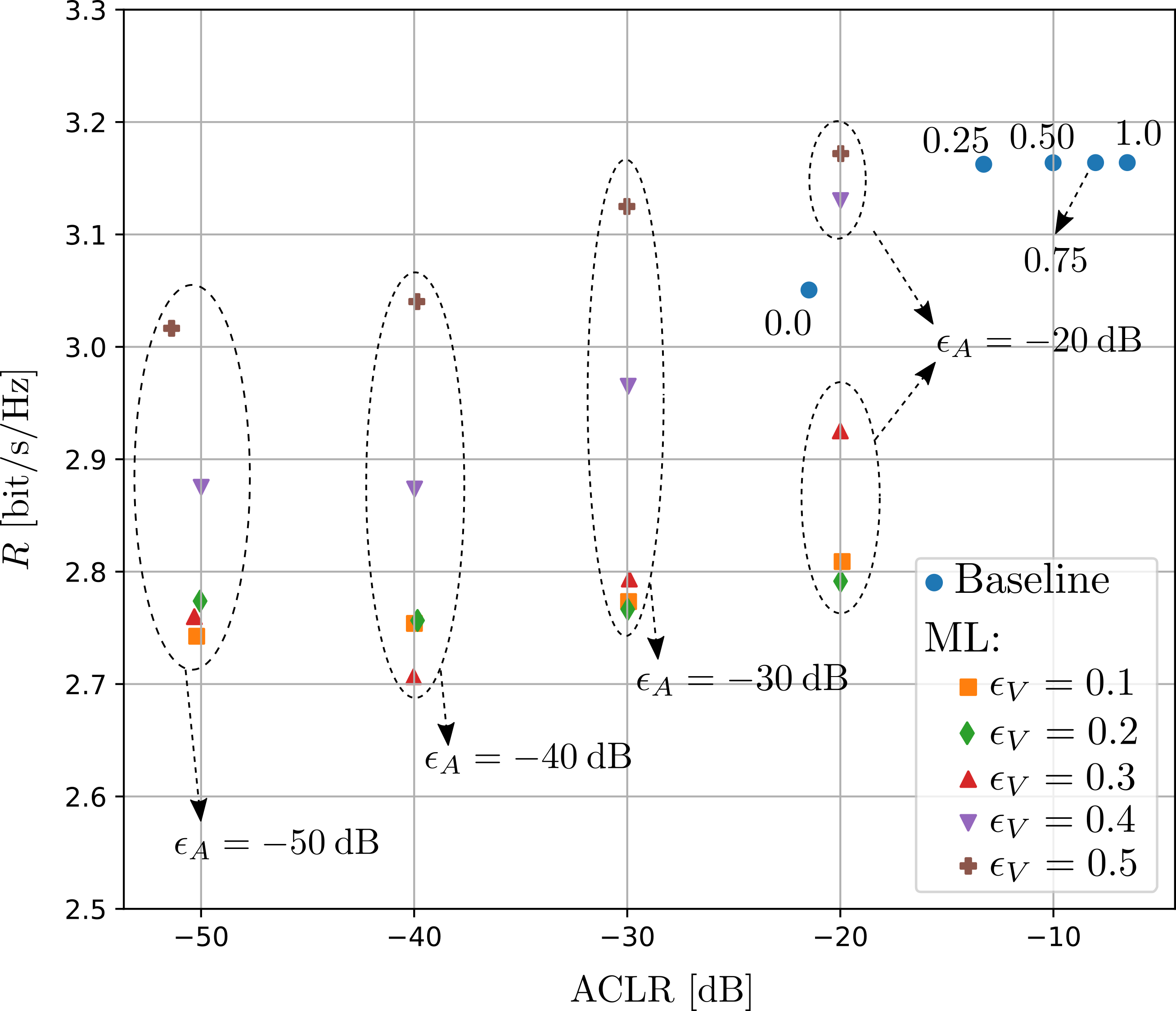
(a) ACLRs and rates achieved by the compared schemes.The roll-off factor value is indicated near each point for the baseline.

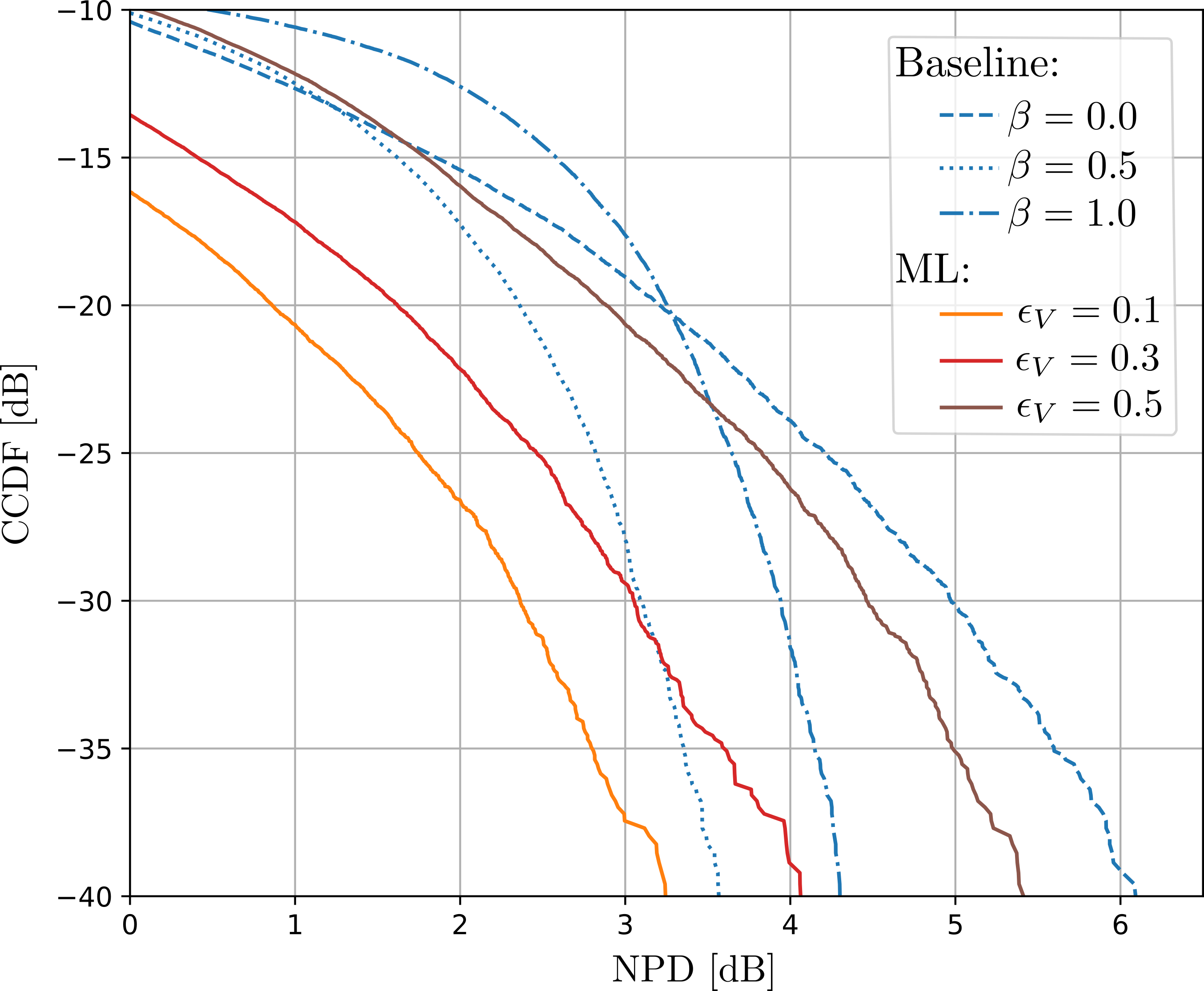
(b) CCDF of the NPD of the baseline and ML schemes for $\epsilon_{A}=-30\>$dB.

Figure 3: Rate, ACLR, and NPD achieved by the baseline and ML schemes.

Finding a local optimum of (P) is made challenging by the constraints (Pa)–(Pd). The constraint (Pa) is enforced through the normalization constant $C(\boldsymbol{\theta})$ (25) in (23), and the constraint (Pb) is enforced through the normalization of the constellation (32). To handle the constraints on the ACLR (Pc) and PED (Pd), the augmented Lagrangian method [10, Chapter 17] is used, which, when applied to our setup, is shown in Algorithm 1. The augmented Lagrangian method consists in solving a sequence of unconstrained optimization problems (line 3), each aiming at minimizing the augmented Lagrangian

$${\cal L}_{A}\left({\cal C},\boldsymbol{\theta},\boldsymbol{\psi},\boldsymbol{\gamma};\lambda_{A}^{[u]},\lambda_{V}^{[u]},\eta^{[u]}\right)\coloneqq{\cal L}({\cal C},\boldsymbol{\theta},\boldsymbol{\psi},\boldsymbol{\gamma})\\ -\lambda_{V}^{[u]}\left(V(\boldsymbol{\theta},{\cal C})-\epsilon_{V}\right)-\lambda_{A}^{[u]}\left(\text{ACLR}(\boldsymbol{\theta})-\epsilon_{A}\right)\\ +\frac{\eta}{2}\left(\left(V(\boldsymbol{\theta},{\cal C})-\epsilon_{V}\right)^{2}+\left(\text{ACLR}(\boldsymbol{\theta})-\epsilon_{A}\right)^{2}\right)$$ (36)

where the superscript $[u]$ refers to the $u^{th}$ iteration, $\lambda_{A}$ and $\lambda_{V}$ are the Lagrange multipliers, and $\eta$ a positive penalty parameter that is progressively increased (line 8). At each iteration, minimizing the augmented Lagrangian is approximately achieved through stochastic gradient descent (SGD).

V Evaluation of end-to-end learning

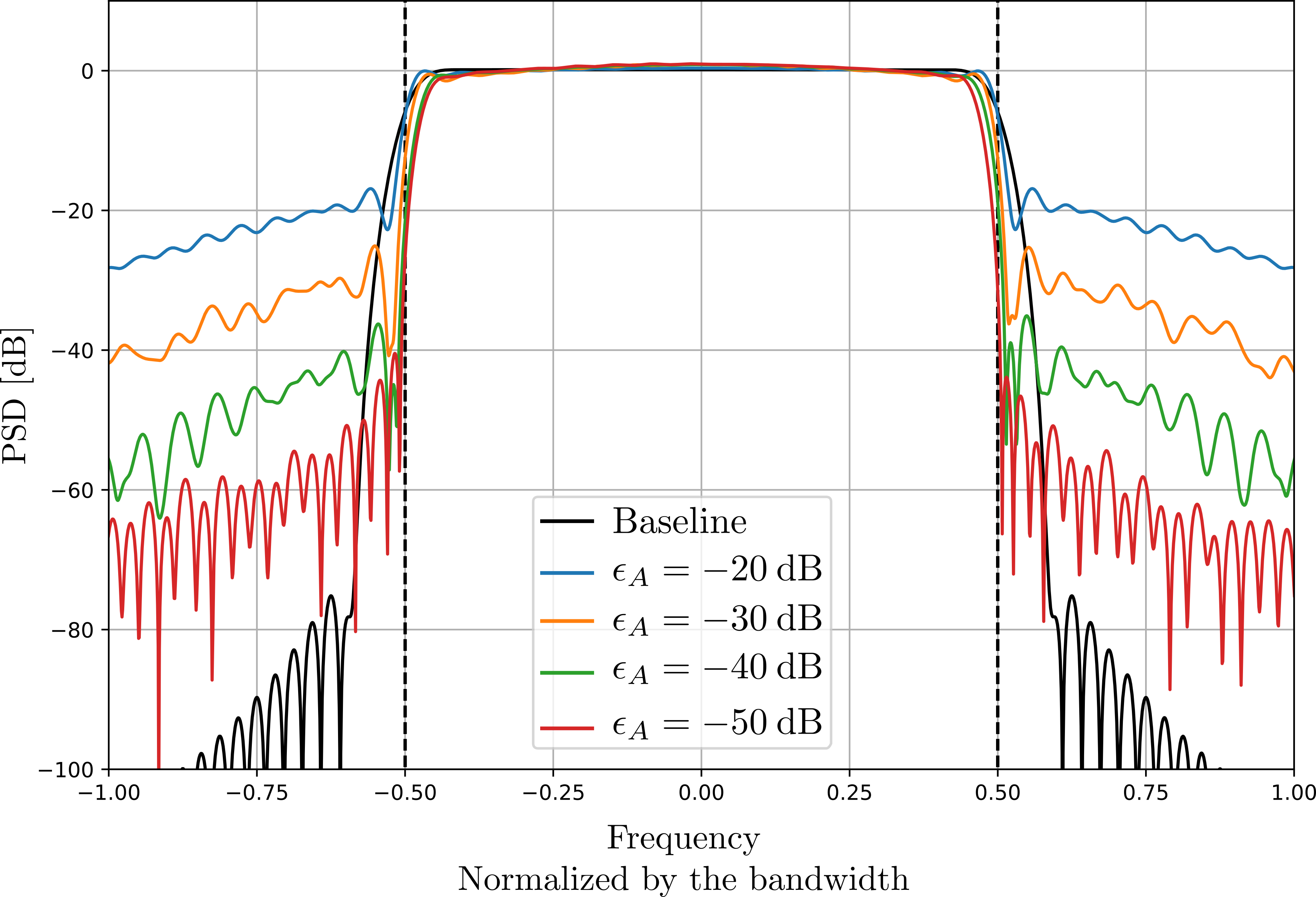
(a) PSD of the baseline and learned filters ($\epsilon_{V}=0.5$).

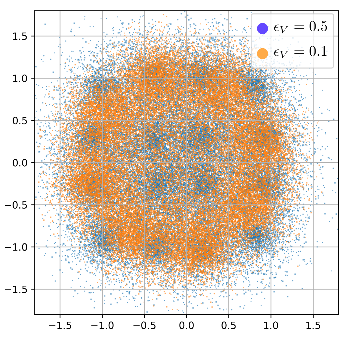
(b) Transmitted signal $x(t)$ ($\epsilon_{A}=-30\>$dB).

Figure 4: Visualization of the transmitted signal with the learned waveform.

We will now present the results of the simulations we have conducted to evaluate the end-to-end learning scheme introduced in the previous section, referred to as the machine learning (ML) scheme. This section first provides details on the training and evaluation setup. The ML scheme is then compared to the baseline.

V-A Evaluation setup

An AWGN channel implemented as described in Section II-A was considered to train and to benchmark the ML scheme against the baseline presented in Section II-B. Note that the approach proposed in Section IV can be applied to any channel model whose output is differentiable with respect to its input, such as multi-paths channels. However, evaluation on such channel models is left for future investigation. The carrier frequency was set to $3.5\>$GHz, and the bandwidth to $W=5\>$MHz. The duration of the transmit and receive filters were set to $D=32T$, and the number of parameters was set to $S=100$ for the trainable filters. The block length was set to $N=990$ symbols, and the modulation order to $16$ ($K=4$). A Gray-labeled 16QAM was used for the baseline. The NN-based receiver operates on the entire block of $N$ symbols. The signal-to-noise ratio (SNR) is defined by $\text{SNR}\coloneqq\frac{1}{N_{0}}$, and was set to $10\>$dB. Training of the ML system was carried out using the Adam [11] optimizer to perform SGD, and with batches of size $M=10$ and a learning rate set to $10^{-3}$. The penalty parameter was initialized to $\eta^{[0]}=10^{-2}$, and increased following a multiplicative schedule $\eta^{[u+1]}=1.2\eta^{[u]}$. The Lagrange multipliers were both initialized to $0$.

V-B Evaluation results

Fig. 3(a) shows the rates $R$ and ACLRs achieved by the baseline and the ML schemes, for different values of $\epsilon_{A}$ and $\epsilon_{V}$. Concerning the baseline, setting the roll-off factor $\beta$ to 0 gives the lowest ACLR, at the cost of a rate loss due to the ISI introduced by the windowing. Higher values of $\beta$ lead to lower ripples making the filter more robust to windowing, at the cost of higher ACLRs. The ML approach, on the other hand, allows accurate control of the ACLR through the parameter $\epsilon_{A}$. Moreover, it enables ACLRs up to $30\>$dB lower than the ones of the baseline, without significant loss of rate assuming high enough values of $\epsilon_{V}$.

The constraint on the PED (Pd) has the strongest impact of the rate $R$. To quantify the impact of this constraint, Fig. 3(b) shows the complementary cumulative distribution function (CCDF) of the normalized power dispersion (NPD),

$$\text{NPD}\coloneqq\frac{\left|p(t)-{\mathbb{E}}\left[p(t)\right]\right|}{{\mathbb{E}}\left[p(t)\right]}.$$ (37)

As one can see, for the lowest values of $\epsilon_{V}$, the ML scheme achieves the lowest NPD, at the cost of a rate loss (Fig. 3(a)). This leads to a PAPR of $7.53\>$dB for the baseline when $\beta=0$, whereas for $\epsilon_{V}=0.4$ and $\epsilon_{A}=-30\>$dB, the ML approach achieves a PAPR of $6.45\>$dB, while enabling a significantly smaller ACLR and a higher rate.

Fig. 4(a) shows the power spectral density (PSD) of the learned filters ($\epsilon_{V}=0.5$) and of the baseline ($\beta=0$). As expected, the learned filter emits less in the adjacent bands, especially for low values of $\epsilon_{A}$, which translates into lower ACLRs. Concerning the constraint on the PED, Fig. 4(b) shows samples from the transmitted signal $x(t)$ for two different values of $\epsilon_{V}$. As one can see, with low values of $\epsilon_{V}$, the samples are concentrated in a “doughnut-like” shape, corresponding to a constant envelope signal, and which would lead to a higher power amplifier efficiency.

VI Conclusion

We have presented an end-to-end learning method for learning waveforms through joint optimization of constellation and pulse shaping to maximize an achievable information rate, with constraints on the ACLR and power envelope. Our simulations results show that the proposed approach enables lower ACLR and less dispersive power envelopes while maintaining competitive rates. Moreover, the end-to-end leaning method does not incur any additional complexity on the transmitter side, as it relies on conventional architectures, and can be applied to any channel model. The presented results are therefore promising for evaluation on other channel models and to design waveforms for emerging beyond 5G services.

References

- [1] H. Viswanathan and P. E. Mogensen, “Communications in the 6G Era,” IEEE Access, vol. 8, pp. 57 063–57 074, 2020.
- [2] S. Cammerer, F. Ait Aoudia, S. Dörner, M. Stark, J. Hoydis, and S. ten Brink, “Trainable communication systems: Concepts and prototype,” IEEE Transactions on Communications, vol. 68, no. 9, pp. 5489–5503, 2020.
- [3] B. Karanov, M. Chagnon, F. Thouin, T. A. Eriksson, H. Bülow, D. Lavery, P. Bayvel, and L. Schmalen, “End-to-End Deep Learning of Optical Fiber Communications,” J. Lightw. Technol., vol. 36, no. 20, pp. 4843–4855, Oct. 2018.
- [4] A. Caciularu, N. Raviv, T. Raviv, J. Goldberger, and Y. Be’ery, “perm2vec: Attentive Graph Permutation Selection for Decoding of Error Correction Codes,” IEEE J. Sel. Areas Commun., vol. 39, no. 1, pp. 79–88, 2021.
- [5] F. Ait Aoudia and J. Hoydis, “Trimming the Fat from OFDM: Pilot-and CP-less Communication with End-to-end Learning,” in Proc. IEEE Globecom Workshops (GC Wkshps) (to appear), 2021.
- [6] J. G. Proakis, M. Salehi, N. Zhou, and X. Li, Communication Systems Engineering. Prentice Hall New Jersey, 1994, vol. 2.
- [7] G. Böcherer, “Achievable Rates for Probabilistic Shaping,” preprint arXiv:1707.01134, 2017.
- [8] T. O’Shea and J. Hoydis, “An Introduction to Deep Learning for the Physical Layer,” IEEE Trans. Cogn. Commun. Netw., vol. 3, no. 4, pp. 563–575, Dec. 2017.
- [9] K. He, X. Zhang, S. Ren, and J. Sun, “Deep Residual Learning for Image Recognition,” in Proc. IEEE Conf. on Comput. Vision and Pattern Recognit. (CVPR), June 2016.
- [10] J. Nocedal and S. Wright, Numerical Optimization. Springer Science & Business Media, 2006.
- [11] D. P. Kingma and J. Ba, “Adam: A Method for Stochastic Optimization,” preprint arXiv:1412.6980, 2014.