Three-dimensional lattice SU($N_{c}$) gauge theories
with multiflavor scalar fields in the adjoint representation

Abstract

We consider three-dimensional lattice SU($N_{c}$) gauge theories with multiflavor ($N_{f}>1$) scalar fields in the adjoint representation. We investigate their phase diagram, identify the different Higgs phases with their gauge-symmetry pattern, and determine the nature of the transition lines. In particular, we study the role played by the quartic scalar potential and by the gauge-group representation in determining the Higgs phases and the global and gauge symmetry-breaking patterns characterizing the different transitions. The general arguments are confirmed by numerical analyses of Monte Carlo results for two representative models that are expected to have qualitatively different phase diagrams and Higgs phases. We consider the model with $N_{c}=3$, $N_{f}=2$ and with $N_{c}=2$, $N_{f}=4$. This second case is interesting phenomenologically to describe some features of cuprate superconductors.

I Introduction

Gauge symmetries represent a fundamental feature of high-energy particle theories Weinberg-book ; Wilson-74 ; ZJ-book and of emerging phenomena in condensed matter physics Wegner-71 ; ZJ-book ; Sachdev-19 ; Anderson-book . It is therefore important to understand the role they play in gauge models. In particular, it is crucial to have a solid understanding of how they relate to global symmetries and of their role in determining the phase structure of the model, the nature of its different Higgs phases and of its quantum and thermal transitions.

We address these issues in three-dimensional (3D) lattice gauge models with multicomponent scalar fields. We consider a lattice model with O($N_{f}$) global invariance, SU($N_{c}$) local invariance, and in which the scalar-matter field transforms in the adjoint representation of SU($N_{c}$) and in the fundamental representation of O($N_{f}$)  GG-72 ; FS-79 . This model is of direct phenomenological interest. In particular, the gauge model with $N_{c}=2$ and $N_{f}=4$ has been proposed as an effective model for optimal doping criticality in hole-doped cuprate superconductors SSST-19 ; SPSS-20 .

Studies addressing the interplay between global and gauge non-Abelian symmetries in 3D models have been already reported. We mention Refs. BPV-19 ; BPV-20 that studied models with fields transforming under the fundamental representation of the gauge group: Ref. BPV-19 studied a model with a local SU($N_{c}$) and a global SU($N_{f}$) invariance and Ref. BPV-20 studied a model with global O($N_{f}$) and local SO($N_{c}$) invariance. Other studies have focused on Abelian U(1) gauge theories HLM-74 ; MZ-03 , such as the lattice Abelian-Higgs model with compact PV-19-AH3d ; WBJSS-05 ; KNS-02 ; MHS-02 ; KKLP-98 and noncompact BPV-21-nc ; HBBS-13 ; KMPST-08 ; MV-08 gauge fields, and with higher-charge scalar fields BPV-20-hc ; WBJS-08 ; CIS-06 ; CFIS-05 ; NSSS-04 ; SSNHS-03 ; SSSNH-02 .

In this paper we extend these studies. First, we investigate the role played by the gauge-group representation of the scalar fields. In particular, we consider lattice SU($N_{c}$) gauge theories with multiflavor scalar matter in the adjoint representation. Second, we consider a generic quartic scalar potential, obtaining a richer phase diagram with different Higgs phases. We mention that some results for this model have been already reported in Ref. SPSS-20, , which discusses the phase diagram and the different Higgs phases for $N_{c}=2$ and $N_{f}=4$. We extend here those results, presenting a numerical analysis of the nature of the phase transitions along the transition lines that separate the different phases. We also mention that the phase behavior of the same model has been studied also in two dimensions BFPV-21 , finding that the asymptotic zero-temperature behavior (continuum limit) is the same as in models defined on symmetric spaces that have the same global symmetry BHZ-80 .

The phase diagram of the lattice SU($N_{c}$) gauge model with multiflavor scalar matter in the adjoint representation depends on the number of colors $N_{c}$ and flavors $N_{f}$. Its low-temperature Higgs phases are essentially determined by the nature of the scalar configurations in the low-temperature limit, and also by the topological properties of the gauge fields. In particular, qualitatively different behaviors emerge for $N_{f}\leq N_{c}^{2}-1$ and $N_{f}>N_{c}^{2}-1$. In the first case there is only one low-temperature Higgs phase, while the second case presents various low-temperature Higgs phases. Correspondingly, we observe transitions that are related to the breaking of the global symmetry group acting on the scalar fields, and topological transitions separating phases with different topological properties of the gauge field. We present numerical studies based on Monte Carlo simulations for one representative of each class of models. We study the model for $N_{c}=3$ and $N_{f}=2$—in this case we have $N_{f}<N_{c}^{2}-1$—and for $N_{c}=2$ and $N_{f}=4$, for which $N_{f}>N_{c}^{2}-1$. Some numerical results for $N_{c}=2$ and $N_{f}=4$ in the strong gauge-coupling limit were also reported in Ref. SPSS-20, .

The model with one scalar field, i.e., with $N_{f}=1$, is also phenomenologically interesting—it is relevant for electron-doped cuprates SSST-19 . However, its phase diagram is somewhat trivial, as it presents a single thermodynamical phase, with two continuously-connected regimes, a disordered-like and a Higgs-like regime DHKR-02 ; SSST-19 . Indeed, the existence of a distinct low-temperature Higgs phase generally requires the breaking of a global symmetry group, which is only possible for $N_{f}\geq 2$.

The paper is organized as follows. In Sec. II we define the lattice SU($N_{c}$) gauge model with $N_{f}$ scalar fields in the adjoint representation. In Sec. III we introduce the observables and discuss their finite-size scaling (FSS) behavior, which will be at the basis of our numerical analyses. In Sec. IV we determine the minimum-potential configurations, which specify the different Higgs phases, and characterize the global and gauge symmetry-breaking patterns. In Sec. V we discuss the renormalization-group (RG) flow of the statistical field theory that is associated with the lattice model, focusing on the case $N_{c}=2$. In Sec. VI we discuss some limiting cases, corresponding to simpler models for which some features of the phase diagram are already known. The next two sections are dedicated to the presentation of the numerical results. In Sec. VII we discuss the phase diagram of the model with $N_{c}=3$ and $N_{f}=2$, which is a representative of models with $N_{f}\leq N_{c}^{2}-1$. Sec. VIII reports a numerical analysis of the more interesting case with $N_{c}=2$ and $N_{f}=4$, for which $N_{f}>N_{c}^{2}-1$. Finally, in Sec. IX we summarize and draw our conclusions. Some details on the MC simulations and numerical analyses are reported in App. A.

II Lattice SU($N_{c}$) gauge models with adjoint scalar fields

We consider lattice gauge models that are invariant under local SU($N_{c}$) and global O($N_{f}$) transformations, with scalar fields that transform under the adjoint representation of SU($N_{c}$) and under the fundamental representation of the O($N_{f}$) group. They are defined on cubic lattices of linear size $L$ with periodic boundary conditions. The fundamental variables are real matrices $\Phi^{af}_{\bm{x}}$, with $a=1,...,N_{c}^{2}-1$ (color index) and $f=1,...,N_{f}$ (flavor index), defined on the lattice sites, and gauge fields $U_{{\bm{x}},\mu}\in{\rm SU}(N_{c})$ associated with the lattice links Wilson-74 . The partition function is

$$Z=\sum_{\{\Phi,U\}}e^{-\beta H}\,,\qquad\beta=1/T\,,$$ (1)

$$H=H_{K}(\Phi,U)+H_{V}(\Phi)+H_{G}(U)\,,$$ (2)

where the lattice Hamiltonian $H$ is the sum of the kinetic term $H_{K}$ of the scalar fields, of the local scalar potential $H_{V}$, and of the pure-gauge Hamiltonian $H_{G}$. As usual, we set the lattice spacing equal to one, so that all lengths are measured in units of the lattice spacing.

The kinetic term $H_{K}$ is given by

$$H_{K}(\Phi,U)=-J{N_{f}\over 2}\sum_{{\bm{x}},\mu}{\rm Tr}\,\Phi_{\bm{x}}^{t}\,\widetilde{U}_{{\bm{x}},\mu}\,\Phi_{{\bm{x}}+\hat{\mu}}^{\phantom{t}}\,,$$ (3)

where the matrix $\widetilde{U}^{ab}_{{\bm{x}},\mu}$ is the adjoint representation of the original link variable $U_{{\bm{x}},\mu}$, explicitly defined as

$$\widetilde{U}^{ab}_{{\bm{x}},\mu}=2\,{\rm Tr}(\,U^{\dagger}_{{\bm{x}},\mu}T^{a}U_{{\bm{x}},\mu}T^{b}\,)\,,\quad a,b=1,...,N_{c}^{2}-1\,,$$ (4)

where $T^{a}$ are the $N_{c}^{2}-1$ generators in the fundamental representation, normalized so that ${\rm Tr}\,T^{a}T^{b}=\frac{1}{2}\delta^{ab}$. In the following we fix $J=1$, so that energies are measured in units of $J$.

The scalar potential term $H_{V}$ is written as

$$H_{V}(\Phi)=\sum_{\bm{x}}V(\Phi_{\bm{x}})\,,$$ (5)

$$V(\Phi)={r\over 2}\,{\rm Tr}\,\Phi^{t}\Phi+{u\over 4}\,\left({\rm Tr}\,\Phi^{t}\Phi\right)^{2}+{v\over 4}\,{\rm Tr}\,(\Phi^{t}\Phi)^{2}\,,$$

which is the most general quartic potential invariant under O($N_{f}$)$\otimes$O($N_{c}^{2}-1$) transformations. For $v=0$, the symmetry group of $H_{V}(\Phi)$ is larger, namely, the O($M$) group with $M=N_{f}(N_{c}^{2}-1)$.

Finally, the pure-gauge plaquette term reads

$$H_{G}(U)=-{\gamma\over N_{c}}\sum_{{\bm{x}},\mu>\nu}{\rm Re}\,{\rm Tr}\,\Pi_{{\bm{x}},\mu\nu}\,,$$ (6)

$$\Pi_{{\bm{x}},\mu\nu}=U_{{\bm{x}},\mu}\,U_{{\bm{x}}+\hat{\mu},\nu}\,U_{{\bm{x}}+\hat{\nu},\mu}^{\dagger}\,U_{{\bm{x}},\nu}^{\dagger}\,,$$

where the parameter $\gamma$ plays the role of inverse gauge coupling.

The model is invariant under global O($N_{f}$) transformations, $\Phi^{af}\to\sum_{g}O^{fg}\Phi^{ag}$, and under local SU($N_{c}$) transformations

$$U_{{\bm{x}},\mu}\to V_{\bm{x}}U_{{\bm{x}},\mu}V_{{\bm{x}}+\hat{\mu}}^{\dagger}\qquad\Phi^{af}_{\bm{x}}\to\sum_{b}\widetilde{V}_{\bm{x}}^{ab}\Phi^{bf}_{\bm{x}},$$ (7)

where $V_{\bm{x}}$ is an SU($N_{c}$) matrix and $\widetilde{V}_{\bm{x}}$ is the corresponding matrix in the adjoint representation [$\widetilde{V}$ can be obtained from $V$ using the analogue of Eq. (4)].

In our study we focus on a representative model with fixed-length scalar fields $\Phi_{\bm{x}}$, satisfying

$${\rm Tr}\,\Phi_{\bm{x}}^{t}\Phi_{\bm{x}}=2\,.$$ (8)

Formally, this model can be obtained by taking the limit $u,r\to\infty$ keeping the ratio $r/u=-2$ fixed. The corresponding lattice Hamiltonian reads

$$H=-{N_{f}\over 2}\sum_{{\bm{x}},\mu}{\rm Tr}\,\Phi_{\bm{x}}^{t}\,\widetilde{U}_{{\bm{x}},\mu}\,\Phi_{{\bm{x}}+\hat{\mu}}^{\phantom{t}}$$ (9)

$$\quad+{v\over 4}\sum_{\bm{x}}{\rm Tr}\,(\Phi_{\bm{x}}^{t}\Phi_{\bm{x}})^{2}-{\gamma\over N_{c}}\sum_{{\bm{x}},\mu>\nu}{\rm Re}\,{\rm Tr}\,\Pi_{{\bm{x}},\mu\nu}\,.$$

Models with generic values of $r$ and $u$ are expected to have the same qualitative behavior as this simplified model.

For $\gamma=0$ each matrix $U_{{\bm{x}},\mu}$ can be multiplied by an arbitrary $({\bm{x}},\mu)$-dependent element of the gauge-group center ${\mathbb{Z}}_{N_{c}}$ without changing the Hamiltonian, thus implying that the gauge group is SU($N_{c}$)$/{\mathbb{Z}}_{N_{c}}$. In particular, this implies $\langle{\rm Tr}\,\Pi_{{\bm{x}},\mu\nu}\rangle=0$ for $\gamma=0$. Note also that, for $N_{c}=2$ and again for $\gamma=0$, because of the isomorphism SU$(2)/{\mathbb{Z}}_{2}=$SO(3), we recover an SO(3) gauge theory with scalar matter in the fundamental representation.

For $\gamma\neq 0$, the gauge Hamiltonian breaks the previous symmetry. However, the Hamiltonian is still invariant under a subgroup of those transformations. More precisely, it is invariant under the transformations $U_{{\bm{x}},\mu}\to c(x_{\mu})U_{{\bm{x}},\mu}$, where $c(x_{\mu})$ is an element of the gauge-group center that depends only on $x_{\mu}$ (the component $\mu$ of the position vector). When this symmetry is not spontaneously broken, Wilson loops obey the area law and color charges transforming in the fundamental representation are confined.

Finally, for $\gamma\to\infty$, the link variables $U_{{\bm{x}},\mu}$ become equal to the identity, modulo gauge transformations. Thus, one recovers a matrix scalar model which is invariant under global O($N_{f}$)$\otimes$O($N_{c}^{2}-1$) transformations [for $v=0$, the global symmetry group is O($M$) with $M=N_{f}(N_{c}^{2}-1)$]. This is strictly true only for an infinite system. On a finite lattice with periodic boundary conditions, it is not possible to set $U_{{\bm{x}},\mu}=1$ on all links and therefore, one ends up with a scalar model with SU($N_{c}$) (since the fields transform under the adjoint representation, the group is more precisely SU($N_{c}$)/${\mathbb{Z}}_{N_{c}}$) fluctuating boundary conditions (see Ref. BPV-21-ccb for a discussion in the context of U(1) gauge models).

III Observables, order parameter and finite-size scaling

To investigate the phase diagram of the lattice SU($N_{c}$) gauge theory (9), we consider the energy density and the specific heat, defined as

$$E=-\frac{1}{3L^{3}}\langle H\rangle\,,\quad C_{V}=\frac{1}{L^{3}}\left(\langle H^{2}\rangle-\langle H\rangle^{2}\right)\,.$$ (10)

The critical properties of the scalar fields can be monitored by using the correlation functions of the gauge-invariant bilinear operators

$$B_{\bm{x}}^{fg}={1\over 2}\sum_{a}\Phi_{\bm{x}}^{af}\Phi_{\bm{x}}^{ag}\,,\qquad Q_{\bm{x}}^{fg}=B_{\bm{x}}^{fg}-{1\over N_{f}}\delta^{fg}\,,$$ (11)

which satisfy ${\rm Tr}\,B_{\bm{x}}=1$ and ${\rm Tr}\,Q_{\bm{x}}=0$ due to the fixed-length constraint. The bilinear scalar operator $Q_{\bm{x}}$ provides the natural order parameter for the breaking of the global O($N_{f}$) symmetry. As we use periodic boundary conditions for all fields, translation invariance holds. We define the two-point correlation function

$$G({\bm{x}}-{\bm{y}})=\langle{\rm Tr}\,Q_{\bm{x}}Q_{\bm{y}}\rangle\,,$$ (12)

the corresponding susceptibility $\chi=\sum_{\bm{x}}G({\bm{x}})$, and the second-moment correlation length

$$\xi^{2}={1\over 4\sin^{2}(\pi/L)}{\widetilde{G}({\bm{0}})-\widetilde{G}({\bm{p}}_{m})\over\widetilde{G}({\bm{p}}_{m})}\,,$$ (13)

where $\widetilde{G}({\bm{p}})=\sum_{{\bm{x}}}e^{i{\bm{p}}\cdot{\bm{x}}}G({\bm{x}})$ is the Fourier transform of $G({\bm{x}})$, and ${\bm{p}}_{m}=(2\pi/L,0,0)$. We also consider RG-invariant quantities, such as the Binder parameter

$$U=\frac{\langle\mu_{2}^{2}\rangle}{\langle\mu_{2}\rangle^{2}}\,,\qquad\mu_{2}=\frac{1}{L^{6}}\sum_{{\bm{x}},{\bm{y}}}{\rm Tr}\,Q_{\bm{x}}Q_{\bm{y}}\,,$$ (14)

and

$$R_{\xi}=\xi/L\,.$$ (15)

At continuous transitions RG-invariant quantities, generically denoted by $R$, scale as PV-02

$$R(\beta,L)=f_{R}(X)+L^{-\omega}g_{R}(X)+\ldots\,,$$ (16)

where

$$X=(\beta-\beta_{c})L^{1/\nu}\,,$$ (17)

and next-to-leading scaling corrections have been neglected. The function $f_{R}(X)$ is universal up to a multiplicative rescaling of its argument, $\nu$ is the critical exponent associated with the diverging correlation length, and $\omega$ is the exponent associated with the leading irrelevant operator. In particular, $U^{*}\equiv f_{U}(0)$ and $R_{\xi}^{*}\equiv f_{R_{\xi}}(0)$ are universal, depending only on the boundary conditions and aspect ratio of the lattice. Since $R_{\xi}$ defined in Eq. (15) is an increasing function of $\beta$, we can write

$$U(\beta,L)=F(R_{\xi})+O(L^{-\omega})\,,$$ (18)

where $F(x)$ depends on the universality class, boundary conditions, and lattice shape, without any nonuniversal multiplicative factor. Eq. (18) is particularly convenient to test universality-class predictions, as it permits a direct comparison of results for different models without requiring a tuning of nonuniversal parameters.

The Binder parameter $U$ is also useful to identify weak first-order transitions, especially when large lattices are required to obtain evidence of a finite latent heat or of a bimodal energy distribution. Indeed, at a first-order transition, the maximum $U_{\rm max}$ of $U$ increases as the volume $L^{3}$, i.e. CLB-86 ; VRSB-93 ; CPPV-04

$$U_{\rm max}=a\,L^{3}+O(1)\,.$$ (19)

This is the key point which distinguishes first-order from continuous transitions. Indeed, at a continuous phase transition, $U$ is finite as $L\to\infty$; at the critical point $U$ converges to a universal value $U^{*}$, while the data of $U$ corresponding to different values of $R_{\xi}$ collapse onto a scaling curve as the volume is increased. Therefore, $U$ has a qualitatively different scaling behavior for first- and second-order transitions. The absence of a data collapse in plots of $U$ versus $R_{\xi}$ may be considered as an early indication of the first-order nature of the transition PV-19 . To identify the transition, one can also consider the specific heat. At first-order transitions, its maximum value $C_{\rm max}(L)$ asymptotically increases as CLB-86

$$C_{\rm max}(L)={\Delta_{h}^{2}\over 4}\,L^{3}+O(1)\,,$$ (20)

where $\Delta_{h}$ is the latent heat, defined as the difference $\Delta_{h}=E(\beta\to\beta_{c}^{+})-E(\beta\to\beta_{c}^{-})$. Moreover, the value of $\beta$ corresponding to the maximum converges to the critical value $\beta_{c}$ as $\beta_{{\rm max},C}(L)-\beta_{c}\approx c\,L^{-3}$. Note that $C_{\rm max}(L)$ may also diverge at continuous transitions (this occurs when $\alpha>0$), and therefore the identification of the order of the transition from the behavior of $C_{\rm max}(L)$ requires a detailed analysis of its asymptotic large-$L$ behavior.

IV Higgs phases

The lattice gauge models we consider may have different Higgs phases associated with different symmetry-breaking patterns. They are determined by the minima of the local scalar potential (5), namely

$$V(\Phi)={v\over 4}\,{\rm Tr}\,(\Phi^{t}\Phi)^{2}\,,$$ (21)

in the fixed-length limit ${\rm Tr}\,\Phi^{t}\Phi=2$. In the following we summarize (using the notations of Ref. BFPV-21 ) the main properties of these phases, which crucially depend on the number of colors $N_{c}$, of flavors $N_{f}$, and on the parameter $v$ SPSS-20 ; SSST-19 ; BFPV-21 . Moreover, as we shall see, their nature may also depend on the behavior of the fluctuations of variables associated with the gauge-group center ${\mathbb{Z}}_{N_{c}}$, which are expected to undergo a transition at finite values of $\gamma>0$.

IV.1 The model for $v<0$

For $v<0$ the mininum-potential configurations can be generally written as SSST-19 ; BFPV-21

$$\Phi^{af}=\sqrt{2}\,s^{a}z^{f}\,,$$ (22)

where ${\bm{s}}$ and ${\bm{z}}$ are unit real vectors of dimension $N^{2}_{c}-1$ and $N_{f}$, respectively. To identify the symmetry breaking pattern at the transition, we should identify the stabilizer group (little group in Wigner’s notation) of the solution (22), i.e., the group of O($N_{f}$) transformations that leave the field (22) invariant, modulo gauge transformations. Explicitly, we should find the orthogonal matrices $O^{fg}$ such that

$$\sum_{g}O^{fg}s^{a}z^{g}=\sum_{b}\widetilde{V}^{ab}s^{b}z^{f}\,,$$ (23)

for some $V\in\hbox{SU}(N_{c})$ (the tilde accent indicates the adjoint representation). It is immediate to verify that $V$ should satisfy $|\sum_{ab}s^{a}\widetilde{V}^{ab}s^{b}|=1$, so that Eq. (23) can be written as

$$\sum_{g}O^{fg}z^{g}=\pm z^{f}\,.$$ (24)

The invariance group is therefore ${\mathbb{Z}}_{2}\otimes O(N_{f}-1)$ and the global symmetry breaking pattern is

$$O(N_{f})\to{\mathbb{Z}}_{2}\otimes O(N_{f}-1)\,.$$ (25)

We also define a gauge-symmetry breaking pattern as the stabilizer of the minimum-potential solution with respect to the gauge group. For this purpose, we determine the matrices $V\in\hbox{SU}(N_{c})$ such that

$$\sum_{b}\widetilde{V}^{ab}s^{b}=s^{a}\,.$$ (26)

Defining $\hat{T}=\sum_{a}s^{a}T^{a}$, and using Eq. (4) we obtain

$$2\sum_{a}T^{a}\hbox{Tr}\,(V^{\dagger}T^{a}V\hat{T})=\hat{T}\,.$$ (27)

Using the completeness relation for the generators, we end up with the condition $[V,\hat{T}]=0$. The stabilizer subgroup is therefore ${\rm U}(1)\oplus{\rm U}(N_{c}-2)$, so that for $v<0$ we observe a gauge symmetry breaking pattern

$${\rm SU}(N_{c})\to{\rm U}(1)\otimes{\rm U}(N_{c}-2)\,,$$ (28)

independently of the flavor number $N_{f}$. In particular, for $N_{c}=2$, we have SPSS-20 SU(2)$\to$U(1) [equivalently, disregarding discrete subgroups, it corresponds to O(3)$\to$O(2)]. Note that we are not claiming here that the gauge symmetry is broken in the standard statistical-mechanics sense (i.e., that we can force the system in one specific minimum, for instance, by appropriately fixing the boundary conditions), as this is forbidden by well-known rigorous arguments Elitzur-75 ; DFG-78 ; BN-87 . The right-hand side of the gauge-symmetry breaking pattern only represents the residual gauge symmetry of the minimum-potential configuration once the scalar fields have been fixed to a specific value by means of an appropriate gauge-fixing condition (see Ref. BN-87 for a discussion of the role of gauge fixings), i.e., once a specific value of $s$ in Eq. (22) has been chosen.

One may also establish a correspondence between the critical behavior of the SU($N_{c}$) gauge model (9) and the 3D RP${}^{N_{f}-1}$ model BFPV-21 . Consider indeed the limit $v\to-\infty$ at fixed $\beta$ and $J$. In this limit $B_{\bm{x}}$, defined in Eq. (11), becomes

$$B_{\bm{x}}^{fg}=z_{\bm{x}}^{f}z_{\bm{x}}^{g}\,,$$ (29)

i.e., it corresponds to a local projector onto a one-dimensional subspace. If we now assume that the dynamics in the gauge model is determined by the fluctuations of the order parameter $B_{\bm{x}}$, or equivalently of $Q_{\bm{x}}$, we identify the effective scalar model as the RP${}^{N_{f}-1}$ model. Indeed, the standard nearest-neighbor RP^N-1 action is obtained by taking the simplest action for a local projector $P^{fg}_{\bm{x}}$:

$$H_{\rm RP}=-J\sum_{{\bm{x}},\mu}\hbox{Tr}\,P_{\bm{x}}P_{{\bm{x}}+\hat{\mu}}\,,\qquad P_{\bm{x}}^{fg}=\varphi_{\bm{x}}^{f}\varphi_{\bm{x}}^{g}\,,$$ (30)

where $\varphi^{a}_{\bm{x}}$ is a unit vector. We do not expect the limit $v\to-\infty$ to be relevant. The crucial property should be the structure of the low-temperature configurations, and thus we expect RP${}^{N_{f}-1}$ in the whole phase in which the symmetry-breaking patterns (25) and (28) hold. We recall that 3D RP^N-1 models undergo continuous transitions only for $N=2$—they belong to the XY universality class. For any $N>2$, transitions are of first order, as predicted by the Landau-Ginzburg-Wilson (LGW) theory PTV-18 ; FMSTV-05 .

IV.2 The model for $v>0$

The behavior of the model is more complex for $v>0$. The minimum-potential configurations can be parametrized as SSST-19 ; BFPV-21

$$\Phi^{ag}=\sqrt{2\over q}\sum_{k=1}^{q}C^{ak}F^{kg}\,,\quad q={\rm Min}[N_{f},N_{c}^{2}-1]\,,$$ (31)

where $C$ and $F$ are orthogonal matrices of dimension $N_{c}^{2}-1$ and $N_{f}$, respectively. To further simplify this expression we should distinguish two cases: $N_{f}\leq N_{c}^{2}-1$ and $N_{f}>N_{c}^{2}-1$

For $N_{f}\leq N_{c}^{2}-1$, we can simplify Eq. (31) into

$$\Phi^{ag}=\sqrt{2\over q}\,C^{ag}\,,\qquad C\in{\rm O}(N_{c}^{2}-1)\,.$$ (32)

Moreover, for $N_{c}=2$, since the adjoint representation of SU(2) is equivalent to SO(3), one may further simplify the representation of the mininum-potential configuration: all such configuration are obtained by applying gauge transformations to $\Phi^{ag}=\sqrt{2/q}\,\delta^{ag}$.

The global invariance group of the ordered phase is given by those transformations $O\in\hbox{O}(N_{f})$ such that

$$\sum_{g}O^{fg}C^{ag}=\sum_{b}\widetilde{V}^{ab}C^{bf},$$ (33)

for some SU($N_{c}$) matrix $V$. This condition implies that $O^{fg}=(C^{t}\widetilde{V}^{t}C)^{fg}$. Since the matrix $C^{t}\widetilde{V}^{t}C$ is an element of the adjoint representation of SU($N_{c}$), $O$ should be an $N_{f}\times N_{f}$ submatrix of an element of $\hbox{SU}(N_{c})_{\rm adj}$. We write the corresponding global symmetry breaking pattern as

$$\hbox{O}(N_{f})\to\hbox{O}(N_{f})\cap\hbox{SU}(N_{c})_{\rm adj}.$$ (34)

For $N_{f}=2$ and 3, since $\hbox{SU}(N_{c})_{\rm adj}$ includes $\hbox{SU}(2)_{\rm adj}=\hbox{SO}(3)$ and inversion transformations on the first $N_{f}$ components, we have $\hbox{O}(N_{f})\cap\hbox{SU}(N_{c})_{\rm adj}=\hbox{O}(N_{f})$. Thus, there is no global symmetry breaking, and thus no transition is expected. These conclusions are consistent with the more general argument presented in Ref. BFPV-21 . It was noted that the gauge-invariant order parameter $Q$ defined in Eq. (11) vanishes if the fields are given by Eq. (31), as it does in the disordered phase. Thus, the system is not expected to have low-temperature phases in which the gauge-invariant bilinear operator $Q$ condenses.

For $N_{f}>N_{c}^{2}-1$, the minimum-potential configurations can be parametrized as BFPV-21

$$\Phi^{ag}=\sqrt{2\over q}\,F^{ag}\,,\qquad F\in{\rm O}(N_{f})\,.$$ (35)

Modulo global O($N_{f}$) transformations, a simple representative is $\Phi^{ag}=\sqrt{2/q}\,\delta^{ag}$. For what concerns the global-symmetry breaking pattern, the transformations $O\in\hbox{O}(N_{f})$ that leave the minimum-potential configurations invariant modulo gauge transformations satisfy the condition $O^{ab}=\widetilde{V}^{ab}$, so that the symmetry-breaking pattern is

$$\hbox{O}(N_{f})\to\hbox{O}(N_{f}-N^{2}_{c}+1)\oplus\hbox{SU}(N_{c})_{\rm adj}\,.$$ (36)

For $N_{c}=2$, it becomes

$$\hbox{O}(N_{f})\to\hbox{O}(N_{f}-3)\oplus\hbox{SO}(3)\,.$$ (37)

If we additionally set $N_{f}=4$, it becomes $\hbox{O}(4)\to\hbox{O}(3)$, which is the symmetry breaking pattern of the O(4) vector model. If we consider the gauge group, instead, since the only matrix that leaves $\Phi^{ag}=\sqrt{2/q}\,\delta^{ag}$ invariant is $\widetilde{V}=1$, the stabilizer group is the center ${\mathbb{Z}}_{N_{c}}$. The gauge symmetry breaking pattern is therefore

$$\hbox{SU}(N_{c})\to{\mathbb{Z}}_{N_{c}}\,.$$ (38)

In the previous discussion we have characterized the phases on the basis of the different minima of the potentials. However, phases may also depend on topological properties of the gauge fields, which are controlled by the coupling $\gamma$. In particular, the modes related to the center of the gauge group ${\mathbb{Z}}_{N_{c}}$ may undergo a confining-deconfining phase transition at finite values of $\gamma$, giving rise to low-temperature Higgs phases that have the same global and local gauge symmetry breaking patterns, but differing for the topological nature of the gauge-center excitations. We expect these phenomena to be relevant for $v>0$, when the gauge symmetry breaking pattern is ${\rm SU}(N_{c})\rightarrow{\mathbb{Z}}_{N_{c}}$, so that the minimum-potential configurations are only invariant under the gauge-group center.

To understand the role of the gauge-group center, we consider the limit $\beta\to\infty$ keeping $\kappa\equiv\beta\gamma$ fixed. In this limit, the relevant configurations minimize the potential and the scalar kinetic energy $H_{K}$. As discussed in Ref. BFPV-21 , for $v>0$ the minimization of $H_{K}$ implies $\widetilde{U}_{{\bm{x}},\mu}=1$, so that $U_{{\bm{x}},\mu}=\lambda_{{\bm{x}},\mu}\in{\mathbb{Z}}_{N_{c}}$. In this limit, model (9) reduces to the lattice ${\mathbb{Z}}_{N_{c}}$ gauge theory

$$H_{{\mathbb{Z}}_{N_{c}}}=-\kappa\sum_{{\bm{x}},\mu>\nu}{\rm Re}\,\lambda_{{\bm{x}},\mu}\,\lambda_{{\bm{x}}+\hat{\mu},\nu}\,\bar{\lambda}_{{\bm{x}}+\hat{\nu},\mu}\,\bar{\lambda}_{{\bm{x}},\nu}\,.$$ (39)

In three dimensions, this lattice discrete gauge model undergoes a continuous transition at a finite $\kappa_{c}$ (see Sec VI.4 for more details). For example, for $N_{c}=2$ the Hamiltonian (39) corresponds to a lattice ${\mathbb{Z}}_{2}$ gauge theory Wegner-71 , which presents a small-$\kappa$ confined phase and a large-$\kappa$ deconfined phase (which may carry topological order at the quantum level Sachdev-19 ), separated by a critical point at $\kappa_{c}=0.761413292(11)$ (see Sec. VI.4). If the ${\mathbb{Z}}_{N_{c}}$ gauge transition persists for finite values of $\beta$, then, when varying $\gamma$, we may have different low-temperature Higgs phases that are associated with the same gauge-symmetry pattern ${\rm SU}(N_{c})\rightarrow{\mathbb{Z}}_{N_{c}}$ but that differ in the large-scale behavior of the ${\mathbb{Z}}_{N_{c}}$ variables. This may lead to a change of the nature of the phase transition from the disordered to the Higgs phases when $N_{f}>N_{c}^{2}-1$, or give rise to observable effects on the scalar correlations for $N_{f}\leq N_{c}^{2}-1$, which are not expected to order for $v>0$.

V RG flow of the gauge field theory

In this section we discuss the RG flow of the statistical field theory corresponding to the lattice model (2), focusing on the case $N_{c}=2$. The starting point is a scalar theory in which the fundamental field is a real matrix $\Phi_{af}$ ($a=1,...,N_{c}^{2}-1$ and $f=1,...,N_{f}$), transforming as the corresponding lattice field (see Sec. II). The corresponding Hamiltonian includes all field monomials of dimension less or equal to four that are invariant under global O($N_{f}$)$\otimes$O($N_{c}^{2}-1$) transformations. To obtain a model invariant under SU($N_{c}$) gauge transformations, we add an SU($N_{c}$) gauge field $A_{\mu}^{a}$ and set ${\cal A}_{\mu\,ab}\equiv iA_{\mu}^{k}T_{A,ab}^{k}$, where $T_{A,ab}^{k}=-if^{abk}$ are the SU($N_{c}$) generators in the adjoint representation ($f^{abc}$ are the structure constants of the SU($N_{c}$) group). The Hamiltonian density is

$${\cal H}={1\over 4g_{0}^{2}}(F^{k}_{\mu\nu})^{2}+(\partial_{\mu}\Phi_{af}+{\cal A}_{\mu\,ab}\Phi_{bf})^{2}+{1\over 2}r\,{\rm Tr}\,\Phi^{t}\Phi$$

$$\;\;+{1\over 4}u_{0}({\rm Tr}\,\Phi^{t}\Phi)^{2}+{1\over 4}v_{0}\left[{\rm Tr}\,(\Phi^{t}\Phi)^{2}-({\rm Tr}\,\Phi^{t}\Phi)^{2}\right]\qquad$$ (40)

where $F_{\mu\nu}^{k}$ is the non-Abelian field strength associated with the gauge field $A_{\mu}^{k}$. To determine the nature of the transitions described by the continuum SU($N_{c}$) gauge theory (40), one studies the RG flow determined by the $\beta$ functions of the model in the coupling space.

In the $\epsilon$-expansion framework, the RG flow close to four dimensions is determined by the one-loop $\overline{\rm MS}$ $\beta$ functions. Introducing the renormalized couplings $u$, $v$, and $\alpha=g^{2}$, the one-loop $\beta$ functions for $N_{c}=2$ are given by SSST-19

$$\beta_{u} = -\epsilon u+{3N_{f}+8\over 6}u^{2}$$

$$+{N_{f}-1\over 3}(v^{2}-2uv)-3u\alpha+{9\over 4}\alpha^{2}\,,$$

$$\beta_{v} = -\epsilon v+{N_{f}-5\over 6}v^{2}+2uv-3v\alpha+{9\over 8}\alpha^{2}\,,$$

$$\beta_{\alpha} = -\epsilon\alpha+{N_{f}-22\over 12}\alpha^{2}\,,$$

where $\epsilon\equiv 4-d$. The normalizations of the couplings can be easily inferred from the above expressions. The $\beta$-functions (V) have a stable fixed point for sufficiently large $N_{f}$, more precisely for $N_{f}>N^{*}+O(\epsilon)$ with $N^{*}\approx 210.5$. In particular, in the large-$N_{f}$ limit the $\beta$ functions can be written in terms of the large-$N_{f}$ parameters $\hat{u}\equiv N_{f}u$, $\hat{v}\equiv N_{f}v$, $\hat{\alpha}\equiv N_{f}\alpha$, as

$$\beta_{\hat{u}}=-\epsilon\hat{u}+{1\over 6}\hat{u}^{2}+{1\over 3}(\hat{u}-\hat{v})^{2}\,,$$ (42)

$$\beta_{\hat{v}}=-\epsilon\hat{v}+{1\over 6}\hat{v}^{2}\,,\quad\beta_{\hat{\alpha}}=-\epsilon\hat{\alpha}+{1\over 12}\hat{\alpha}^{2}\,,$$

which have a stable fixed point located at

$$\hat{\alpha}^{*}=12\epsilon\,,\quad\hat{u}^{*}=6\epsilon\,,\quad\hat{v}^{*}=6\epsilon\,.$$ (43)

Note that the stable fixed point in the large-$N_{f}$ limit is located in the region $v>0$. Thus, it should describe the continuous transitions between the disordered phase and the positive-$v$ Higgs phase discussed in Sec. IV.2.

VI Some particular cases

In this section we discuss some particular cases of the gauge model (9), which correspond to lattice models that have already been studied in the literature. This analysis will provide us some indications on the phase diagram of the full theory.

VI.1 The model for $N_{c}=2$, $\gamma=0$, and $v=0$

For $N_{c}=2$ and $\gamma=0$, the model (9) is equivalent to a lattice SO(3) gauge model with $N_{f}$ scalar flavors in the fundamental representation. The Hamiltonian is

$$H=-{N_{f}\over 2}\sum_{{\bm{x}},\mu}{\rm Tr}\,\Phi_{\bm{x}}^{t}\,V_{{\bm{x}},\mu}\,\Phi_{{\bm{x}}+\hat{\mu}}^{\phantom{t}}+{v\over 4}\sum_{\bm{x}}{\rm Tr}\,(\Phi_{\bm{x}}^{t}\Phi_{\bm{x}})^{2}\,,$$ (44)

where the link variables $V_{{\bm{x}},\mu}$ belong to the fundamental representation of the gauge group SO(3). For $v=0$ this model was discussed in Ref. BPV-20 . It was predicted that, for any $N_{f}$, the system undergoes a finite-temperature transition which is the same as in the corresponding RP${}^{N_{f}-1}$ model, cf. Eq. (30). Therefore, one predicts a continuous XY transition for $N_{f}=2$ and a first-order transition for any $N_{f}>2$. Indeed, in the LGW Hamiltonian appropriate for the RP${}^{N_{f}-1}$ model PTV-18 ; FMSTV-05 , a cubic $\Phi^{3}$ term is always present for $N_{f}>2$, a presence which is usually considered as an indication of a first-order transition for 3D statistical models.

These predictions have been confirmed numerically BPV-20 . For $N_{f}=2$ there is a continuous XY transition at $\beta_{c}=1.97690(7)$, while for $N_{f}=3$ there is a first-order transition at $\beta_{c}\approx 1.77$. These numerical results indicate that, for $v=0$, the relevant low-temperature configurations are those of the form (22), that correspond to the minima of the potential for $v<0$.

VI.2 The limit $\gamma\to\infty$

For $\gamma\to\infty$ the variables $U_{{\bm{x}},\mu}$ converge to the identity, apart from gauge transformations. Thus, we obtain the scalar model

$$H=-{N_{f}\over 2}\sum_{{\bm{x}},\mu}{\rm Tr}\,\Phi_{\bm{x}}^{t}\,\Phi_{{\bm{x}}+\hat{\mu}}^{\phantom{t}}+{v\over 4}\sum_{\bm{x}}{\rm Tr}\,(\Phi_{\bm{x}}^{t}\Phi_{\bm{x}})^{2}\,,\quad$$ (45)

with a global O($N_{f}$)$\otimes$O($N_{c}^{2}-1$) symmetry. For $v=0$, the symmetry group is larger, namely O($M$) with $M=N_{f}(N_{c}^{2}-1)$, and therefore we expect continuous transitions belonging to the O($M$) vector universality class. For $v\neq 0$, the models (45) may undergo a finite-temperature continuous transition only if a corresponding universality class exists and, in particular, only if the corresponding LGW $\Phi^{4}$ theory has a stable fixed point. RG analyses indicate that continuous transitions are possible for $N_{f}=2$ and $N_{c}=2$  Kawamura-98 ; PRV-01 ; PV-02 ; Parruccini-03 ; CPPV-04 ; DPV-04 ; NO-14 ; HKS-20 , for both $v<0$ and $v>0$, and for DPV-06 $N_{f}=4$ and $N_{c}=2$ when $v<0$. Moreover, for $v>0$ there is a stable fixed point for sufficiently large $N_{f}$ at fixed $N_{c}$ and sufficiently large $N_{c}$ at fixed $N_{f}$ (in particular for $N_{c}=2$ and any $N_{f}$) PRV-01-ln ; Kawamura-98 ; CPPV-04 . It is not clear whether the fixed points of the O($N_{f}$)$\otimes$O($N_{c}^{2}-1$) field theory are relevant for the behavior for finite values of $\gamma$. For instance, the O($M$) fixed point that controls the behavior for $\gamma=\infty$ and $v=0$ is unstable with respect to the gauge coupling, and is therefore irrelevant for the finite-$\gamma$ behavior, although it is expected to give crossover effects for large values of $\gamma$. There are at present no analogous results for $v\not=0$.

VI.3 The limit $\beta\to\infty$

In the limit $\beta\to\infty$ the behavior of the system is controlled by the configurations minimizing the Hamiltonian. As already discussed in Sec. IV, two different low-temperature phases occur for $v<0$ and $v>0$. Therefore, in this limit we expect a transition line for $v=0$ and any $\gamma$. The transition line should be of first order for any $N_{f}$ and $N_{c}$, as it separates phases that correspond to different minima of the potential.

VI.4 The limit $\beta\to\infty$ keeping $\kappa\equiv\beta\gamma$ fixed

Let us now consider the limit $\beta\to\infty$ keeping $\kappa\equiv\beta\gamma$ fixed. As mentioned in Sec. IV.2, for $v>0$ the model (9) reduces to the lattice ${\mathbb{Z}}_{N_{c}}$ gauge theory defined in Eq. (39). This model can be related by duality to the $N_{c}$-state clock spin model SSNHS-03 , characterized by a global ${\mathbb{Z}}_{N_{c}}$ symmetry. For $q=2$, the $q$-state clock model is equivalent to the standard Ising model and thus we expect an Ising transition. Duality allows us to obtain $\kappa_{c}$ for $N_{c}=2$: $\kappa_{c}={1\over 2}\ln\coth\beta_{I,c}$, where $\beta_{I,c}$ is the inverse temperature of the Ising model. Using FXL-18 $\beta_{I,c}=0.221654626(5)$, we obtain $\kappa_{c}=0.761413292(11)$. For $q=3$, the $q$-state clock model is equivalent to a three-state Potts model, which can only undergo first-order transitions. For larger values of $q$, we expect a continuous transition. It belongs to the Ising universality class for HS-03 $q=4$, and to the 3D XY universality class for HS-03 ; Hasenbusch-19 ; PSS-20 $q\geq 5$. Note, however, that in the $q\to\infty$ limit we recover the pure U(1) gauge theory, with $\lambda_{{\bm{x}},\mu}\in{\rm U}(1)$, which is known QED to have no transitions for finite values of $\kappa$. Therefore, if a transition occurs for any finite $q$, we must have $\kappa_{c}\to\infty$ in the $q\to\infty$ limit.

Since for $v>0$ and $N_{f}>N_{c}^{2}-1$ the low-temperature Higgs phase is characterized by the gauge-symmetry breaking pattern ${\rm SU}(N_{c})\rightarrow{\mathbb{Z}}_{N_{c}}$ (see Sec. IV.2), it seems natural to expect that the confinement-deconfinement center transition also persists for finite $\beta$, giving rise to two different positive-$v$ Higgs phases, depending on $\gamma$.

For $v<0$, the low-temperature Higgs phase is characterized by a residual continuous gauge symmetry, see Eq. (28). Since 3D pure gauge theories with continuous gauge group do not display any confinement-deconfinement transition, the same is expected to happen for the model (9) when $v<0$.

VI.5 The limit $v\to\pm\infty$

For $|v|\to\infty$, configurations are constrained to be minima of the the scalar potential (21). For $v\to+\infty$, the scalar fields take the form (31), reducing the model to a particular $\sigma$ model. Transitions are expected for $N_{f}>N_{c}^{2}-1$, with the global symmetry-breaking pattern (36) [or (37) for $N_{c}=2$]. For $N_{f}=4$, $N_{c}=2$, the global symmetry-breaking pattern is O(4)$\to$O(3) and therefore the transition should belong to the O(4) vector universality class.

For $v\to-\infty$ scalar variables take the form (29). As discussed in Sec. IV.1, one expects to recover the effective RP${}^{N_{f}-1}$ model (30), whose transitions are continuous for $N_{f}=2$ and of first order for any $N_{f}>2$.

VII Results for $N_{c}=3$ and $N_{f}=2$

Figure 1: A sketch of the phase diagram for $N_{c}=3$, $N_{f}=2$, and $\gamma=0$, inferred from the numerical results.

In this section we determine the phase diagram for $N_{f}=2$, $N_{c}=3$, and $\gamma=0$. According to the discussion reported in Sec. VI.3, since $N_{f}<N^{2}_{c}-1$, for $\beta=\infty$ there is only one ordered Higgs phase, which is obtained for $v<0$. For finite values of $\beta$ we expect therefore only two phases: a disordered phase and an ordered Higgs phase, separated by a single transition line. As discussed in Sec. IV, the transitions between the disordered and Higgs phases should be described by an effective RP¹ model, which is equivalent to the XY model for ${\mathbb{Z}}_{2}$ gauge-invariant observables. Therefore, such transitions should belong to the XY universality class PV-02 , if they are continuous. The transition line is expected to approach the point $v=0$ in the $\beta=+\infty$ limit. Moreover, since this ending point should correspond to a first-order transition as outlined in Sec. VI.3, we expect the transition line to become of first order for large values of $\beta$. The phase diagram obtained from our MC simulations, see Fig. 1, is fully consistent with these considerations. Note that the transition line intersects the line $v=0$ at a finite $\beta$ value, so that the ordered Higgs phase is also present for finite-$\beta$ positive values of $v$. Of course, the transition line should be reentrant, since $v_{c}\to 0^{+}$ for $\beta\to\infty$.

To verify the phase diagram sketched in Fig. 1, we have performed simulations for $v=0$ varying $\beta$, and at fixed $\beta$ (we have considered $\beta=5.2$, 6, 7.5, 9, 12) varying $v$. We have verified the reentrant nature of the transition line and that the transition changes from a continuous one to a first-order one as $\beta$ increases (the tricritical point, where the order of the transition changes, should satisfy $6\lesssim\beta_{\rm tri}\lesssim 7.5$). Some technical details on the MC simulations are reported in App. A.

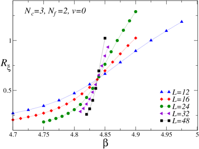
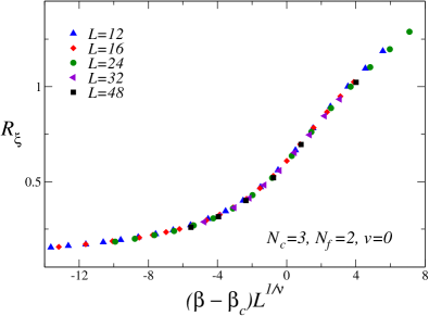
Figure 2: Top: Plot of $R_{\xi}$ versus $\beta$ for $N_{c}=3$, $N_{f}=2$, $\gamma=0$, and $v=0$. Bottom: Plot of $R_{\xi}$ versus $(\beta-\beta_{c})L^{1/\nu}$, using the XY correlation-length exponent $\nu=0.6717$ and $\beta_{c}=4.8374$. Data collapse on an asymptotic curve with increasing $L$.

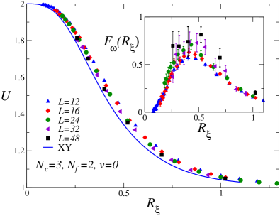
Figure 3: Plot of $U$ versus $R_{\xi}$ for $N_{c}=3$, $N_{f}=2$, $\gamma=0$, and $v=0$. The continuous line represents the universal curve $F(R_{\xi})$ for the XY universality class (the explicit expression is reported in Ref. BPV-21-ccb ; it is valid in the range $[0,1.1]$ with an error of at most $0.5\%$). The inset shows $[U-F(R_{\xi})]L^{\omega}$ versus $R_{\xi}$, using the XY correction-to-scaling exponent $\omega=0.789$. Data show a reasonable scaling behavior as predicted by Eq. (46).

The FSS analysis of the data at $v=0$ and $\gamma=0$, see Figs. 2 and 3, provides a clear evidence of a continuous transition at $\beta_{c}\approx 4.84$. If we plot $R_{\xi}$ versus $(\beta-\beta_{c})L^{1/\nu}$, using the XY correlation-length exponent CHPV-06 ; Hasenbusch-19 ; CLLPSSV-19 $\nu=0.6717(1)$, we obtain an excellent collapse of the data, confirming that the transition belongs to the XY universality class. Fits of $R_{\xi}$ using the XY estimate for the critical exponent $\nu$ lead to an accurate estimate of the critical point, $\beta_{c}=4.8374(2)$. The best evidence for an XY critical behavior is provided by the plots of $U$ versus $R_{\xi}$. The data approach the universal curve of the XY universality class obtained by MC simulations of the standard XY model. Differences get smaller and smaller with increasing $L$. Moreover, see the inset of Fig. 3, deviations are consistent with the expected FSS scaling behavior

$$U(L,R_{\xi})-F(R_{\xi})\approx L^{-\omega}F_{\omega}(R_{\xi})\,,$$ (46)

where $F(R_{\xi})$ is the universal curve associated with the XY universality class, $\omega=0.789(4)$ is the leading XY scaling correction exponent Hasenbusch-19 , and $F_{\omega}(R_{\xi})$ is a scaling function that is universal apart from a multiplicative factor.

We have also performed simulations at fixed $\beta$, varying $v$. The numerical results show evidence of an XY continuous transition for $\beta=5.2$ and $\beta=6$ (see Fig. 4), at $v_{c}\approx 0.23$ and $v_{c}\approx 0.58$, respectively. On the other hand, we observe first-order transitions for $\beta=7.5$ at $v_{c}\approx 0.99$ (see Fig. 5), for $\beta=9$ at $v_{c}\approx 0.75$, and for $\beta=12$ at $v_{c}\approx 0.45$. Note that these results are consistent with the fact that the transitions become of first order as $\beta$ increases and that $v_{c}\to 0^{+}$ in the limit $\beta\to\infty$ (see Sec. VI.3).

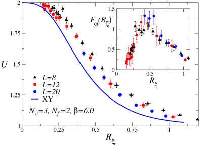
Figure 4: Plot of $U$ versus $R_{\xi}$ for $N_{c}=3,N_{f}=2$, $\gamma=0$, and $\beta=6.0$. The inset shows $[U-F(R_{\xi})]L^{\omega}$ versus $R_{\xi}$, using the XY value $\omega=0.789$, confirming the expected behavior (46). Note also that the data reported in the inset appear to collapse onto a curve which differs from that reported in the inset of Fig. 3 only by a multiplicative factor, in agreement with Eq. (46).

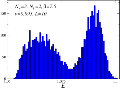
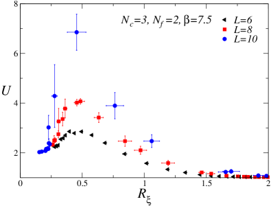
Figure 5: Top: Histogram of the total energy $E$ for $N_{c}=3,N_{f}=2,\beta=7.5,v=0.995$, and $L=10$. Bottom: Binder parameter $U$ versus $R_{\xi}$. Data clearly indicate that the transition is of first order.

We do not expect the phase diagram to change for finite $\gamma>0$, since the main features of the disordered and of the Higgs phase should not depend on $\gamma$. On the other hand, for $\gamma=\infty$, the phase diagram should significantly change, see Sec. VI.2. One expects three different phases: one disordered phase, and two different ordered phases, characterized by different breakings of the global O($N_{f}$)$\otimes$O($N_{c}^{2}-1$) i.e., O(2)$\otimes$O(8) in the case at hand (for $\beta\to\infty$, they would be specified by the sign of $v$). Correspondingly, we expect three transition lines: one line separates the two ordered phases (starting at $\beta=\infty$, $v=0$) and two lines separate the ordered phases from the disordered one. The order-disorder transitions for $v>0$ may be continuous, and associated with the stable fixed point of the corresponding LGW theory PRV-01 ; PRV-01-ln . On the other hand, first-order transitions are expected for $v<0$, since there is no corresponding stable fixed point. We do not expect the $\gamma=\infty$ phases to be stable with respect to the gauge perturbation (this can be proved using the $\epsilon$ expansion for the simpler case $v=0$), and thus the $\gamma=\infty$ transitions should only give rise to crossover effects.

VIII Results for $N_{c}=2$ and $N_{f}=4$

We now present a study of the phase diagram for $N_{f}=4$ and $N_{c}=2$. In this case, since $N_{f}>N_{c}^{2}-1$, according to the arguments of Sec. IV, different Higgs phases caracterized by different gauge-symmetry patterns are possible. For $\beta\to\infty$, they correspond to the behavior of the system for $v<0$ and $v>0$, and thus we will refer to the two phases as the negative-$v$ and positive-$v$ phases, respectively, although, this characterization will not hold for finite $\beta$. For finite $\beta$ the two phases are divided by a transition line that ends at $v=0$, $\beta=\infty$ and which is expected to be of first order as it is the boundary of two different ordered phases.

The structure of the negative-$v$ Higgs phase has been discussed in Sec. IV.1. The global symmetry breaking pattern is $\hbox{O(4)}\to\hbox{O(3)}\oplus{\mathbb{Z}}_{2}$ and the gauge symmetry breaking pattern is $\hbox{SU(2)}\to\hbox{U(1)}$. Since the remnant gauge-invariance group of the Higgs phase is U(1) and a U(1) gauge theory never undergoes phase transitions, we expect the gauge coupling to be irrelevant: we have a single negative-$v$ Higgs phase, irrespective of the value of $\gamma$. As discussed in Sec. IV.1, the transition line separating the negative-$v$ Higgs phase from the disordered phase is expected to be described by the RP³ model, which can only undergo first-order transitions.

Figure 6: Sketch of the phase diagram for $N_{c}=2$, $N_{f}=4$, and $\gamma=0$, as inferred from the numerical results. Thick lines denote first-order transitions, while the thin line corresponds to continuous transitions. The shaded point is a first-order multicritical point (satisfying $1.6<\beta_{mc}<2.5$); the filled black point that separates first-order from continuous transitions occurs at $v=v^{*}$ with $6<v^{*}<12$.

The structure of the positive-$v$ Higgs phase is more interesting. Indeed, the gauge symmetry breaking pattern is $\hbox{SU(2)}\to{\mathbb{Z}}_{2}$, i.e., the Higgs phase is only invariant under the center of the gauge group. Since ${\mathbb{Z}}_{2}$ gauge theories have a finite-temperature transition, we expect $\gamma$ to be relevant, as discussed in Sec. VI.4. Therefore, we may have two different positive-$v$ Higgs phases, which differ for the behavior of the topological modes associated with the gauge-group center SSST-19 ; SPSS-20 . The global symmetry breaking pattern of the positive-$v$ Higgs phase is O(4)$\to$O(3). This would suggest that the continuous transitions between one of the positive-$v$ Higgs phases and the disordered phase belong to the O(4) vector universality class, provided that gauge modes are irrelevant at the transition.

In Fig. 6 we report a sketch of the phase diagram for $\gamma=0$. As already observed for $N_{c}=3$ and $N_{f}=2$, the negative-$v$ phase extends in the positive-$v$ region for intermediate values of $\beta$. The transitions between the two low-temperature phases and between the negative-$v$ and the disordered phases are of first order, as expected. The nature of the transition between the positive-$v$ and the disordered phase depends instead on $v$. At least for $v\lesssim 6$, the transition line is of first order. On the other hand, for large $v$, the transitions become apparently continuous.

To understand the role played by the parameter $\gamma$ for $v>0$, we focus on the phase diagram for a specific positive value of $v$, as a function of $\kappa=\beta\gamma$ and $\beta$. In particular, we consider the relatively large value $v=24$. For this value, at $\gamma=0$, there is a continuous transition between the positive-$v$ Higgs phase and the disorderd phase. A sketch of the phase diagram is reported in Fig. 7. It is characterized by three phases, a small-$\beta$ disordered phase, and two large-$\beta$ Higgs phases, which are distinguished by the behavior of gauge-group center modes. These phases are separated by three transition lines: (i) a disordered-Higgs transition line for small $\kappa$, which appears to be continuous; (ii) a disordered-Higgs transition line for large $\kappa$, which is of first order; (iii) a continuous ${\mathbb{Z}}_{2}$ gauge (Ising) transition line, which separates the two low-temperature Higgs phases.

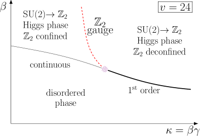
Figure 7: A sketch of the $\beta$-$\kappa$ phase diagram for the model with $N_{c}=2$, $N_{f}=4$ for $v=24$. The ${\mathbb{Z}}_{2}$ gauge transition line starts at $\kappa_{c}\approx 0.761$, $\beta=\infty$. The multicritical point, where the three transition lines meet, satisfies $1<\kappa<2$.

VIII.1 The case $\gamma=0$

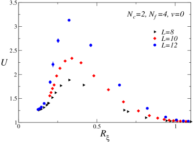
Figure 8: Plot of $U$ versus $R_{\xi}$ for $N_{c}=2$, $N_{f}=4$, $\gamma=0$, and $v=0$. The rapid increase of the maximum of $U$ indicates that the transition is of first order.

To verify that the line that separates the negative-$v$ Higgs phase from the disordered phase is of first order, we have studied the model for $v=0$. A transition is observed for $\beta\approx 1.63$. Since the Binder parameter $U$, reported as a function of $R_{\xi}$ in Fig.8, has a maximum that increases rapidly with the size of the lattice, we conclude that the transition is of first order. To verify that transitions along the line that separates the two Higgs phases are of first order, we have performed simulations at fixed $\beta=2.5$. We observe a transition for $v\approx 2.7$. On both sides of the transition, the Binder parameter $U$ is approximately 1, as expected, while it increases rapidly for $v\approx 2.7$. The transition is of first order as also confirmed by the behavior of the specific heat $C_{V}$, that appears to diverge roughly as the volume $L^{3}$, see Fig. 9.

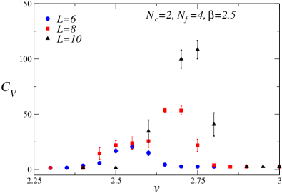
Figure 9: The specific heat, defined in Eq. (10), versus $v$, for $N_{c}=2,N_{f}=4$, $\gamma=0$, and $\beta=2.5$, The data provide evidence of a first-order transition for $v\approx 2.7$.

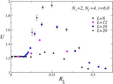
Figure 10: Plot of $U$ versus $R_{\xi}$ for $N_{c}=2$, $N_{f}=4$, $\gamma=0$, and $v=6$. The increase of the maximum of $U$ may be considered as an early indication of a first-order phase transition.

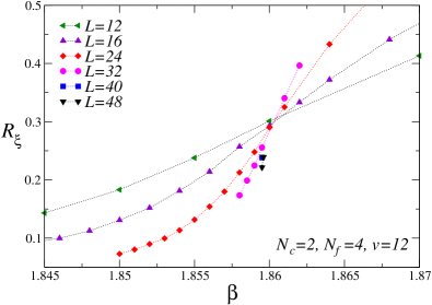
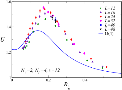
Figure 11: Data for $N_{c}=2,N_{f}=4$, $\gamma=0$ and the values $v=12$. For comparison, we also report the spin-2 universal curve computed in the O(4) vector model footnote-O4curve .

We now focus on the transition line separating the disordered phase from the positive-$v$ Higgs phase, performing simulations at fixed $v$ (we consider $v=6,12,24$, and 48). For $v=6$, we have studied the behavior of the system for $0\leq\beta\leq 3.4$, identifying a single transition for $\beta_{c}\approx 2.04$. This guarantees us that the transition point belongs to the positive-$v$ transition line. The transition appears to be of first order. Indeed, the Binder parameter $U$ has a maximum that increases with increasing lattice size, see Fig. 10. As already mentioned, this behavior provides an early indication for a first-order transition. Indeed, at a continuous transition the maximum of $U$ does not increase.

The results for $v=12$ (up to $L=48$), $v=24$ (up to $L=32$), and $v=48$ (up to $L=24$) are consistent with continuous transitions, see Figs. 11 and 12, located at $\beta_{c}\approx 1.860$, $\beta_{c}\approx 1.710$, and $\beta_{c}\approx 1.618$, respectively. Fits of $R_{\xi}$ allow us to estimate $\nu\approx 0.7$ in all cases, which is quite different from the effective exponent $\nu=1/d\approx 0.33$ expected at first-order transitions. These results confirm the phase diagram reported in Fig. 6: The positive-$v$ transition line is of first order from the multicritical point, where the three transition lines meet, up to a tricritical point $v^{*}$ (with $6\leq v^{*}\leq 12$), and continuous for $v>v^{*}$.

As mentioned in Sec. IV.2, along the transition line dividing the disordered phase from the positive-$v$ Higgs phase, the global symmetry breaking pattern is O(4)$\to$O(3), which is the one characterizing the vector O(4) universality class. One would thus expect O(4) transitions for all $v>v^{*}$. Fits of $R_{\xi}$ give $\nu\approx 0.7$ (with somewhat large errors), which is consistent with the O(4) value $\nu=0.750(2)$ HV-11 ; Deng-06 ; Hasenbusch-01 ; PV-02 . However, the scaling curves of the Binder parameter $U$ versus $R_{\xi}$ are significantly different from the O(4) one, see Figs. 11 and 12. O(4) behavior is apparently possible only if there are slowly-decaying and nonmonotonic scaling corrections. Alternatively, it is possible that the transitions belong to a new universality class. However, one should still explain the significant differences in the behavior of $U$ versus $R_{\xi}$ for $v=12$ and for $v=24$, 48 (compare Figs. 11 and 12). Scaling nonuniversal corrections or crossover effects due to the nearby tricritical point may be invoked as possible reasons. In this scenario, the O(4) fixed point would be unstable, and it would only give rise to crossover phenomena, that apparently become less important as $v$ increases. The available simulations do not allow us to clarify this point. Simulations on significantly larger lattices are clearly required.

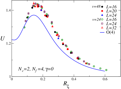
Figure 12: Data for $N_{c}=2,N_{f}=4$, $\gamma=0$ and the values $v=24$ and $v=48$. For comparison, we also report the spin-2 universal curve computed in the O(4) vector model footnote-O4curve .

VIII.2 The case $\gamma>0$

We have also performed a numerical study of the model for $\gamma>0$, focusing on the region $v>0$, where gauge-center modes can give rise to finite-$\gamma$ transitions. We have fixed $v=24$, obtaining the phase diagram reported in Fig. 7. We parametrize the phase diagram in terms of $\kappa\equiv\beta\gamma$ instead of $\gamma$, since this is the natural variable that appears in the ${\mathbb{Z}}_{2}$ gauge model obtained for large values of $\beta$, see Eq. (39). To identify the nature of the disorder-Higgs transitions, we have performed simulations keeping $\kappa$ fixed and varying $\beta$. Since the ${\mathbb{Z}}_{2}$ gauge transition line ends at $\kappa_{c}=0.761$, $\beta=\infty$, we expect the multicritical point to have $\kappa_{mc}$ of order 1, and therefore we have considered $\kappa=1\,,2\,,3$. Finally, we have performed a simulation keeping $\beta$ fixed ($\beta=1.7$) and varying $\kappa$, to determine the position of the ${\mathbb{Z}}_{2}$ gauge transition line and the corresponding universality class.

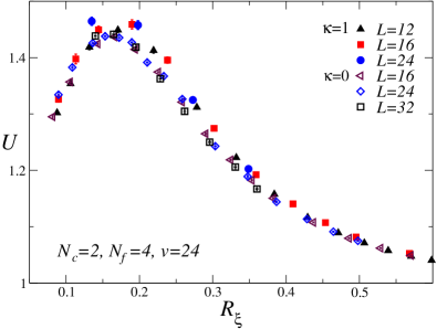
Figure 13: Data of $U$ versus $R_{\xi}$ for $N_{c}=2,N_{f}=4$, $v=24$, and two values of $\kappa$, $\kappa=0$ and 1.

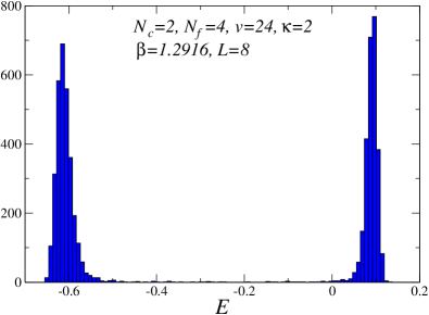
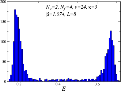
Figure 14: Energy hystograms for $v=24$, $\kappa=2$ (top) and $\kappa=3$ (bottom), for $L=8$. They clearly show the double-peak structure characterizing first-order transitions. The difference of the energies of the two maxima provides the latent heat: $\Delta_{h}\approx 0.7$ for $\kappa=2$, and $\Delta_{h}\approx 0.5$ for $\kappa=3$.

For $\kappa=1$, there is a clear evidence of a continuous transition at $\beta_{c}\approx 1.615$ (correspondingly $\gamma\approx 0.62$). The transition appears to be analogous to that observed for $\gamma=\kappa=0$ at a similar value of $\beta$ ($\beta_{c}\approx 1.710$). In Fig. 13 we report $U$ versus $R_{\xi}$ for $\kappa=0$ and 1. Data are consistent with a single asymptotic curve, suggesting that the two transitions belong to the same universality class. Differences are small, of the same order of the differences observed for the largest $v$ results for $\gamma=0$, and can be interpreted as scaling corrections.

For $\kappa=2$ and 3 we observe instead strong first-order transitions. For example, the energy distributions are bimodal for $\kappa=2$, $\beta_{c}\approx 1.29$ and for $\kappa=3$, $\beta_{c}\approx 1.07$ (correspondingly $\gamma\approx 1.55$ and $\gamma\approx 2.79$) already for lattices sizes $L=6,\,8$, see Fig. 14. The latent heat $\Delta_{h}$ is quite large. It decreases with increasing $\kappa$, varying from $\Delta_{h}\approx 0.7$ at $\kappa=2$ to $\Delta_{h}\approx 0.5$ at $\kappa=3$. This decrease is also confirmed by results for $\kappa=5$: for $L=8$ the energy distribution is broad—therefore it is consistent with a first-order transition—but it does not yet show two peaks. We have also performed some simulations for $\kappa=\gamma=\infty$, i.e., of the scalar model with global O(4)$\otimes$O(3) symmetry, to determine the critical behavior of the endpoint of the finite-$\kappa$ transition line. MC data for relatively small lattices, up to $L=18$, (not shown) are compatible with a continuous transition (larger lattices are however needed to confirm this behavior), indicating that $\Delta_{h}\to 0$ as $\kappa\to\infty$.

The above-reported results show that the nature of the transition changes significantly with increasing $\kappa$. While a continuous transition occurs for $\kappa\lesssim 1$, for $\kappa\geq 2$ transitions are of first order, decreasing their strength with increasing $\kappa$. A natural hypothesis is that this abrupt change is due to the different nature of the Higgs phase: For $\kappa=1$ the low-temperature phase is characterized by confined ${\mathbb{Z}}_{2}$ gauge excitations, while for $\kappa\geq 2$ the ${\mathbb{Z}}_{2}$ gauge modes are deconfined. This requires the existence of the ${\mathbb{Z}}_{2}$ gauge transition line and implies that, in the sketch reported in Fig. 7, the multicritical point lies in the region $1<\kappa_{mc}<2$.

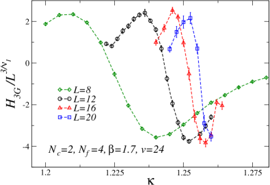
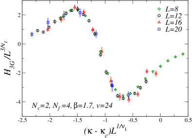
Figure 15: Estimates of $H_{3G}L^{-3/\nu_{I}}$ for $v=24$, $\beta=1.7$, $N_{c}=2$, and $N_{f}=4$, using the Ising exponent $\nu_{I}=0.629971$. The top panel reports $H_{3G}L^{-3/\nu_{I}}$ versus $\kappa$, while the bottom panel reports $L^{-3/\nu}H_{3G}$ versus $L^{1/\nu}(\kappa-\kappa_{c})$, with $\kappa_{c}=1.265$. The plots provide evidence of an Ising transition at $\beta=1.7$ and $\kappa_{c}\approx 1.265$.

We performed simulations to identify the ${\mathbb{Z}}_{2}$ gauge transition line. We fixed $\beta=1.7$ (which is slightly larger than the critical point $\beta_{c}=1.615$ for $\kappa=1$) and varied $\kappa$ between $\kappa=1$ and $\kappa=2$. To determine the ${\mathbb{Z}}_{2}$ gauge transition we monitored thermodynamic quantities, since the transition is not characterized by a local order parameter. We considered cumulants of the gauge part $H_{G}$ of the Hamiltonian, focusing on the second and third cumulant. The second cumulant per unit volume behaves as the specific heat $C_{V}\sim c\,L^{\alpha/\nu}+C_{\rm reg}$, where $C_{\rm reg}$ is the regular contribution. Using the accurate estimates of the 3D Ising critical exponents GZ-98 ; CPRV-02 ; Hasenbusch-10 ; KPSV-16 ; KP-17 ; Hasenbusch-21 , and in particular KPSV-16 $\nu=0.629971(4)$, we obtain $\alpha/\nu=2/\nu-3=0.17475(2)$. The divergence is very mild and scaling corrections (due to the regular background) decay only as $L^{-0.17}$, so that FSS analyses of this quantity are not useful for accurate checks of the Ising behavior. A more promising quantity is the third cumulant of $H_{G}$

$$H_{3G}=-\frac{1}{\gamma^{3}}\langle(H_{G}-\langle H_{G}\rangle)^{3}\rangle\,.$$ (47)

It behaves as $H_{3G}\sim L^{3/\nu}=L^{4.76}$, with scaling corrections that decay as $L^{-\omega}\sim L^{-0.8}$, therefore significantly faster than in the second-cumulant case. We will use the third cumulant to verify the Ising nature of the transition, checking that the data of $L^{-3/\nu}H_{3G}$ asymptotically collapse onto a universal scaling function with a peculiar oscillating shape SSNHS-03 , when they are plotted against $(\kappa-\kappa_{c})L^{1/\nu}$, where $\kappa_{c}$ is the critical point at $\beta=1.7$. This is nicely confirmed by Fig. 15. We have therefore a robust evidence of an Ising transition at $\kappa_{c}\approx 1.265$, (correspondingly $\gamma_{c}=\kappa_{c}/\beta\approx 0.744$).

These results provide evidence for the existence of a finite-$\beta$ ${\mathbb{Z}}_{2}$ transition line, starting at $\kappa_{c}\approx 0.761$, $\beta=\infty$, consistently with the sketch reported in Fig. 7. Moreover, they suggest that the multicritical point lies in the region $1\leq\kappa_{m}\leq 2$, explaining the different behavior observed for $\kappa=1$ and $\kappa=2,3$.

IX Conclusions

We have investigated the phase diagram, and the transitions separating the different phases, of a class of 3D lattice non-Abelian SU($N_{c}$) gauge models with $N_{f}$ ($N_{f}>1$) degenerate scalar fields in the adjoint SU($N_{c}$) representation, using the Wilson formulation of lattice gauge theories, see Eq. (2). These models are also relevant phenomenologically, in particular the model with $N_{c}=2$ and $N_{f}=4$ has been recently proposed to describe optimal doping criticality in cuprate high-$T_{c}$ superconductors SSST-19 ; SPSS-20 .

We discuss the role played by the scalar quartic potential and by the gauge-group representation of the scalar fields, which are crucial to determine the structure of the low-temperature Higgs phases and the nature of the phase transitions. For this purpose we have performed a detailed analysis of the minima of the scalar-field potential. As discussed in Sec. IV, such an analysis shows the emergence of two qualitatively different phase diagrams, depending on the number of colors $N_{c}$ and of flavors $N_{f}$. For $N_{f}\leq N_{c}^{2}-1$ a single Higgs phase exists and, for positive values of $v$ ($v$ is parameter entering the scalar potential (5)), there is a single disordered phase for any temperature up to $T=0$. For $N_{f}>N_{c}^{2}-1$, instead, two different low-temperature Higgs phases exist, with transitions characterized by different global and gauge symmetry breaking patterns. In particular, for $N_{c}=2$, we have a low-temperature Higgs phase characterized by the gauge symmetry breaking pattern ${\rm SU}(2)\to{\rm U}(1)$ (this phase is observed when $v$ is negative), and a second low-temperature Higgs phase characterized by ${\rm SU}(2)\rightarrow{\mathbb{Z}}_{2}$ (this occurs for positive $v$).

The phase diagram of the model can also be influenced by the properties of the gauge modes, depending on the residual gauge symmetry present in the ordered Higgs phase. The phase diagram for $N_{f}\leq N_{c}^{2}-1$ is not expected to depend on the gauge modes, as the residual gauge symmetry group in the Higgs phase is continuous, and therefore no finite-temperature transitions associated with these gauge variables are possible in three dimensions. Thus, the phase diagram should not depend on the gauge coupling $\gamma$. Differences should occur only for $\gamma=\infty$. Analogously, for $N_{f}>N_{c}^{2}-1$, the negative-$v$ Higgs phase should not depend on $\gamma$, given the large residual gauge symmetry characterizing its low-temperature Higgs phase. On the other hand, in the positive-$v$ Higgs phase present for $N_{f}>N_{c}^{2}-1$ configurations are only invariant under gauge-group center transformations. Since ${\mathbb{Z}}_{N_{c}}$ gauge theories undergo finite-temperature transitions, there are two different Higgs phases, characterized by the same gauge-symmetry breaking pattern SU($N_{c}$)$\to{\mathbb{Z}}_{N_{c}}$, but differing in the topological behavior of the ${\mathbb{Z}}_{N_{c}}$ gauge modes. as sketched in Fig. 7 for $N_{c}=2$ and $N_{f}=4$.

We have presented numerical studies of two representative models: the case $N_{c}=3$, $N_{f}=2$, to verify the general scenario for models satisfying $N_{f}\leq N_{c}^{2}-1$, and the case $N_{c}=2$, $N_{f}=4$, which shows the more complex phase diagram predicted for models satisfying $N_{f}>N_{c}^{2}-1$, and which is also relevant for cuprate superconductors. In both cases, the general predictions for the Higgs phases, and for the nature of the transition lines, are verified.

Although our results confirm the general picture, there are still some issues that call for further investigations. For $N_{f}=4$ and $N_{c}=2$, we have evidence of continuous transitions for small values of $\gamma$ and large positive values of $v$, whose characterization is not clear (we have not been able to assign these transitions to a known universality class). A second issue is the behavior for large values of $\gamma$ and of $v$. We have observed first-order transitions, whose latent heat decreases with increasing $\gamma$. It would be interesting to investigate the nature of the endpoint of the transition line at $\gamma=\infty$: numerical simulations on small lattices are consistent with a continuous transition, but larger lattices are needed to settle the question.

An intriguing possibility is that the continuous transitions observed when $N_{f}>N_{c}^{2}-1$, $v>0$ and small values of $\gamma$, are associated with the fixed point found in the analysis of the one-loop $\epsilon$-expansion RG flow, see Sec.V. The $O(\epsilon)$ fixed point in Eq. (43) is stable only if $N_{f}>N^{*}\approx 210$ close to four dimensions. However, it is conceivable that the critical number $N^{*}$ is drastically smaller in three dimensions, so small to include $N_{f}=4$. One might find this possibility unplausible; however, we should note that this is what happens in the Abelian-Higgs U(1) field theory. A leading order $\epsilon$-expansion computation HLM-74 , analogous to the one reported in Sec. V, predicts the existence of a stable fixed point for $N_{f}>N_{f}^{*}\approx 183$. However, if higher-order corrections are included IZMHS-19 , a significantly smaller estimate of the 3D critical value is obtained. A numerical MC study in three dimensions finds $N_{f}^{*}=7(2)$ BPV-21-nc , confirming that the one-loop estimate is of no quantitative relevance. We believe that further work is called for to test this possibility and to achieve a full understanding of the actual behavior of the model for positive values of $v$. A promising strategy consists in studying the model for $v=+\infty$. The model is significantly simpler, since the scalar field variables take the form given in Eq. (21), and simulations faster, as there is no need to take the potential into account in the update and more powerful MC algorithms can be used. This should allow us to perform a more effective numerical study of the phase diagram in the $\beta$-$\gamma$ plane.

Acknowledgement. Numerical simulations have been performed on the CSN4 cluster of the Scientific Computing Center at INFN-PISA.

Appendix A Monte Carlo simulations

We performed MC simulations on cubic lattices with periodic boundary conditions. The gauge link variables $U_{{\bm{x}},\mu}$ were updated using a standard Metropolis algorithm Metropolis:1953am . The new link variable was chosen close to the old one, in order to guarantee an acceptance rate of approximately 30%. The scalar fields were updated using two different Metropolis updates, again tuning the proposal to obtain an acceptance rate of 30%. The first move performs a rotation in flavor space, while the second one rotates the color components of a single flavor. This update procedure is the same already used in BFPV-21 , to which we refer for some more implementation details. For the largest sizes simulated, the typical statistics are of the order of $10^{6-7}$ ($N_{c}=3,N_{f}=2$) and of $10^{7-8}$ ($N_{c}=2,N_{f}=4$) lattice sweeps of both scalar and gauge variables. To take into account autocorrelations and determine the correct statistical errors, we used a standard blocking and jackknife procedure. Our maximum blocking sizes were of the order of $10^{4-5}$ ($N_{c}=3,N_{f}=2$) and $10^{5-6}$ ($N_{c}=2,N_{f}=4$).

References

- (1) S. Weinberg, The Quantum Theory of Fields, (Cambridge University Press, 2005).
- (2) K. G. Wilson, Confinement of quarks, Phys. Rev. D 10, 2445 (1974).
- (3) J. Zinn-Justin, Quantum Field Theory and Critical Phenomena, fourth edition (Clarendon Press, Oxford, 2002).
- (4) F. J. Wegner. Duality in generalized Ising models and phase transitions without local order parameters J. Math. Phys. 12, 2259 (1971).
- (5) S. Sachdev, Topological order, emergent gauge fields, and Fermi surface reconstruction, Rep. Prog. Phys. 82, 014001 (2019).
- (6) P. W. Anderson, Basic Notions of Condensed Matter Physics, (The Benjamin/Cummings Publishing Company, Menlo Park, California, 1984).
- (7) H. Georgi and S. L. Glashow, Unified weak and electromagnetic interactions without neutral currents, Phys. Rev. Lett. 28, 1494 (1972).
- (8) E. Fradkin and S. Shenker, Phase diagrams of lattice gauge theories with Higgs fields, Phys. Rev. D 19, 3682 (1979).
- (9) S. Sachdev, H. D. Scammell, M. S. Scheurer, and G. Tarnopolsky, Gauge theory for the cuprates near optimal doping, Phys. Rev. B 99, 054516 (2019).
- (10) H. D. Scammell, K. Patekar, M. S. Scheurer, and S. Sachdev, Phases of SU(2) gauge theory with multiple adjoint Higgs fields in 21 dimensions, Phys. Rev. B 101, 205124 (2020).
- (11) C. Bonati, A. Pelissetto, and E. Vicari, Phase Diagram, Symmetry Breaking, and Critical Behavior of Three-Dimensional Lattice Multiflavor Scalar Chromodynamics, Phys. Rev. Lett. 123, 232002 (2019); Three-dimensional lattice multiflavor scalar chromodynamics: Interplay between global and gauge symmetries, Phys. Rev. D 101, 034505 (2020).
- (12) C. Bonati, A. Pelissetto, and E. Vicari, Three-dimensional phase transitions in multiflavor scalar SO() gauge theories, Phys. Rev. E 101, 062105 (2020).
- (13) B. I. Halperin, T. C. Lubensky, and S. K. Ma, First-Order Phase Transitions in Superconductors and Smectic-A Liquid Crystals, Phys. Rev. Lett. 32, 292 (1974).
- (14) M. Moshe and J. Zinn-Justin, Quantum field theory in the large limit: A review, Phys. Rep. 385, 69 (2003).
- (15) A. Pelissetto and E. Vicari, Multicomponent compact Abelian-Higgs lattice models, Phys. Rev. E 100, 042134 (2019).
- (16) S. Wenzel, E. Bittner, W. Janke, A. M. J. Schakel, and A. Schiller, Kertesz Line in the Three-Dimensional Compact U(1) Lattice Higgs Model, Phys. Rev. Lett. 95, 051601 (2005).
- (17) H. Kleinert, F. S. Nogueira, and A. Sudbø, Deconfinement Transition in Three-Dimensional Compact U(1) Gauge Theories Coupled to Matter Fields, Phys. Rev. Lett. 88, 232001 (2002).
- (18) S. Mo, J. Hove, and A. Sudbø, Order of the metal-to-superconductor transition, Phys. Rev. B 65, 104501 (2002).
- (19) K. Kajantie, M. Karjalainen, M. Laine, and J. Peisa, Masses and phase structure in the Ginzburg-Landau model, Phys. Rev. B 57, 3011 (1998).
- (20) C. Bonati, A. Pelissetto, and E. Vicari, Lattice Abelian-Higgs models with noncompact gauge field, Phys. Rev. B 103, 085104 (2021).
- (21) E. V. Herland, T. A. Bojesen, E. Babaev, and A. Sudbø, Phase structure and phase transitions in a three-dimensional SU(2) superconductor, Phys. Rev. B 87, 134503 (2013).
- (22) A. B. Kuklov, M. Matsumoto, N. V. Prokof’ev, B. V. Svistunov, and M. Troyer, Deconfined Criticality: Generic First-Order Transition in the SU(2) Symmetry Case, Phys. Rev. Lett. 101, 050405 (2008).
- (23) O. I. Motrunich and A. Vishwanath, Comparative study of Higgs transition in one-component and two-component lattice superconductor models, arXiv:0805.1494 [cond-mat.stat-mech].
- (24) C. Bonati, A. Pelissetto, and E. Vicari, Higher-charge three-dimensional compact lattice Abelian-Higgs models, Phys. Rev. E 102, 062151 (2020).
- (25) S. Wenzel, E. Bittner, W. Janke, and A. M. J. Schakel, Percolation of Vortices in the 3D Abelian Lattice Higgs Model, Nucl. Phys. B 793, 344 (2008).
- (26) M. N. Chernodub, E. M. Ilgenfritz, and A. Schiller, Phase structure of an Abelian two-Higgs model and high-temperature superconductors, Phys. Rev. B 73, 100506(R) (2006).
- (27) M. N. Chernodub, R. Feldmann, E.-M. Ilgenfritz, and A. Schiller, The compact Abelian Higgs model in the London limit: vortex-monopole chains and the photon propagator, Phys. Rev. D 71, 074502 (2005).
- (28) F. S. Nogueira, J. Smiseth, E. Smørgrav, and A. Sudbø, Compact U(1) gauge theories in dimensions and the physics of low dimensional insulating materials, Eur. Phys. J. C 33, 885 (2004).
- (29) J. Smiseth, E. Smørgrav, F. S. Nogueira, J. Hove, and A. Sudbø, Phase Structure of Compact Lattice Gauge Theories and the Transition from Mott Insulator to Fractionalized Insulator, Phys. Rev. B 67, 205104 (2003).
- (30) A. Sudbø, E. Smørgrav, J. Smiseth, F. S. Nogueira, and J. Hove, Criticality in the (2+1)-Dimensional Compact Higgs Model and Fractionalized Insulators, Phys. Rev. Lett. 89, 226403 (2002).
- (31) C. Bonati, A. Franchi, A. Pelissetto, and E. Vicari, Two-dimensional lattice SU(Nc) gauge theories with multiflavor adjoint scalar fields, JHEP 05 (2021) 018.
- (32) E. Brézin, S. Hikami, and J. Zinn-Justin, Generalized non-linear -models with gauge invariance, Nucl. Phys. B 165, 528 (1980).
- (33) A. C. Davis, A. Hart, T. W. B. Kibble, and A. Rajantie, The Monopole mass in the three-dimensional Georgi-Glashow model, Phys. Rev. D 65, 125008 (2002).
- (34) C. Bonati, A. Pelissetto, and E. Vicari, Lattice gauge theories in the presence of a linear gauge-symmetry breaking, [arXiv:2106.02503 [hep-lat]].
- (35) A. Pelissetto and E. Vicari, Critical phenomena and renormalization group theory, Phys. Rep. 368, 549 (2002).
- (36) M. S. S. Challa, D. P. Landau, and K. Binder, Finite-size effects at temperature-driven first-order transitions Phys. Rev. B 34, 1841 (1986).
- (37) K. Vollmayr, J. D. Reger, M. Scheucher, and K. Binder, Finite size effects at thermally-driven first order phase transitions: A phenomenological theory of the order parameter distribution Z. Phys. B 91 113 (1993).
- (38) P. Calabrese, P. Parruccini, A. Pelissetto, and E. Vicari, Critical behavior of O(2)O()-symmetric models, Phys. Rev. B 70, 174439 (2004).
- (39) A. Pelissetto and E. Vicari, Three-dimensional ferromagnetic CPN-1 models, Phys. Rev. E 100, 022122 (2019).
- (40) S. Elitzur, Impossibility of spontaneously breaking local symmetries, Phys. Rev. D 12, 3978 (1975).
- (41) G. F. De Angelis, D. de Falco, and F. Guerra, Note on the abelian Higgs-Kibble model on a lattice: absence of spontaneous magnetization, Phys. Rev. D 17, 1624 (1978).
- (42) C. Borgs and F. Nill, The phase diagram of the abelian lattice Higgs model. A review of rigorous results, J. Stat. Phys. 47, 877 (1987).
- (43) A. Pelissetto, A. Tripodo, and E. Vicari, Criticality of O() symmetric models in the presence of discrete gauge symmetries, Phys. Rev. E 97, 012123 (2018).
- (44) L. A. Fernández, V. Martín-Mayor, D. Sciretti, A. Tarancón, and J. L. Velasco, Numerical study of the enlarged O(5) symmetry of the 3-D antiferromagnetic RP2 spin model, Phys. Lett. B 628, 281 (2005).
- (45) H. Kawamura, J. Phys.: Condens. Matter 10, 4707 (1998).
- (46) A. Pelissetto, P. Rossi, and E. Vicari, The critical behavior of frustrated spin models with noncollinear order, Phys. Rev. B 63, 140414(R) (2001).
- (47) P. Parruccini, Critical behavior of frustrated spin systems with nonplanar orderings, Phys. Rev. B 68, 104415 (2003).
- (48) M. De Prato, A. Pelissetto, and E. Vicari, The normal-to-planar superfluid transition in 3He, Phys. Rev. B 70, 214519 (2004).
- (49) Y. Nakayama and T. Ohtsuki, Approaching the conformal window of O(n)O(m) symmetric Landau-Ginzburg models using the conformal bootstrap, Phys. Rev. D 89, 126009 (2014).
- (50) J. Henriksson, S. R. Kousvos, and A. Stergiou, Analytic and Numerical Bootstrap of CFTs with O(m)O(n) Global Symmetry in 3D, SciPost Phys. 9, 035 (2020)
- (51) M. De Prato, A. Pelissetto, and E. Vicari, Spin-density-wave order in cuprates, Phys. Rev. B 74, 144507 (2006).
- (52) A. Pelissetto, P. Rossi, and E. Vicari, Large- critical behavior of O()O() spin models, Nucl. Phys. B 607, 605 (2001).
- (53) A. M. Ferrenberg, J. Xu, and D. P. Landau, Pushing the limits of Monte Carlo simulations for the three-dimensional Ising model, Phys. Rev. E 97, 043301 (2018).
- (54) J. Hove and A. Sudbø, Criticality versus in the (2+1)-dimensional clock model, Phys. Rev. E 68, 046107 (2003).
- (55) M. Hasenbusch, Monte Carlo study of an improved clock model in three dimensions, Phys. Rev. B 100, 224517 (2019).
- (56) P. Patil, H. Shao, and A. W. Sandvik, Unconventional U(1) to cross-over in quantum and classical q-state clock models, Phys. Rev. B 103, 054418 (2021).
- (57) A. Polyakov, Compact gauge fields and the infrared catastrophe, Phys. Lett. 59B, 82 (1975); for an extensive list of references, see A. Athenodorou and M. Teper, On the spectrum and string tension of U(1) lattice gauge theory in 2 + 1 dimensions, J. High Energy Phys. 01, 063 (2019), and M. Caselle, A. Nada, M. Panero, and D. Vadacchino, Conformal field theory and the hot phase of three-dimensional gauge theory, J. High Energy Phys. 05, 068 (2019).
- (58) M. Campostrini, M. Hasenbusch, A. Pelissetto, and E. Vicari, Theoretical estimates of the critical exponents of the superfluid transition in 4He by lattice methods, Phys. Rev. B 74, 144506 (2006).
- (59) S. M. Chester, W. Landry, J. Liu, D. Poland, D. Simmons-Duffin, N. Su, and A. Vichi, Carving out OPE space and precise O(2) model critical exponents, [arXiv:1912.03324].
- (60) We report here the universal scaling curve computed in the O(4) model. The Binder parameter and the correlation length are defined as in Sec. III, using ( is a 4-dimensional unit vector). The parametrization is valid for with a relative error of less than .
- (61) M. Hasenbusch and E. Vicari, Anisotropic perturbations in 3D O() vector models, Phys. Rev. B 84, 125136 (2011).
- (62) Y. Deng, Bulk and surface phase transitions in the three-dimensional O(4) spin model, Phys. Rev. E 73, 056116 (2006).
- (63) M. Hasenbusch, Eliminating leading corrections to scaling in the three-dimensional O(N)-symmetric model: and 4, J. Phys. A 34, 8221 (2001).
- (64) R. Guida and J. Zinn-Justin, Critical exponents of the N-vector model, J. Phys. A 31, 8103 (1998).
- (65) M. Campostrini, A. Pelissetto, P. Rossi, and E. Vicari, 25th-order high-temperature expansion results for three-dimensional Ising-like systems on the simple-cubic lattice Phys. Rev. E 65, 066127 (2002).
- (66) M. Hasenbusch, A finite size scaling study of lattice models in the three-dimensional Ising universality class, Phys. Rev. B 82, 174433 (2010).
- (67) F. Kos, D. Poland, D. Simmons-Duffin, and A. Vichi, Precision islands in the Ising and O() models, J. High Energy Phys. 08, 036 (2016).
- (68) M. V. Kompaniets and E. Panzer, Minimally subtracted six-loop renormalization of O()-symmetric theory and critical exponents, Phys. Rev. D 96, 036016 (2017).
- (69) M. Hasenbusch, Restoring isotropy in a three-dimensional lattice model: The Ising universality class, arXiv:2105.09781.
- (70) B. Ihrig, N. Zerf, P. Marquard, I. F. Herbut, and M. M. Scherer, Abelian Higgs model at four loops, fixed-point collision and deconfined criticality, Phys. Rev. B 100, 134507 (2019).
- (71) N. Metropolis, A. W. Rosenbluth, M. N. Rosenbluth, A. H. Teller, and E. Teller, Equation of state calculations by fast computing machines, J. Chem. Phys. 21, 1087 (1953).