Meta-learning for Matrix Factorization without Shared Rows or Columns

Abstract

We propose a method that meta-learns a knowledge on matrix factorization from various matrices, and uses the knowledge for factorizing unseen matrices. The proposed method uses a neural network that takes a matrix as input, and generates prior distributions of factorized matrices of the given matrix. The neural network is meta-learned such that the expected imputation error is minimized when the factorized matrices are adapted to each matrix by a maximum a posteriori (MAP) estimation. We use a gradient descent method for the MAP estimation, which enables us to backpropagate the expected imputation error through the gradient descent steps for updating neural network parameters since each gradient descent step is written in a closed form and is differentiable. The proposed method can meta-learn from matrices even when their rows and columns are not shared, and their sizes are different from each other. In our experiments with three user-item rating datasets, we demonstrate that our proposed method can impute the missing values from a limited number of observations in unseen matrices after being trained with different matrices.

1 Introduction

Matrix factorization is an important machine learning technique for imputing missing values and analyzing hidden structures in matrices. With matrix factorization, a matrix is modeled by the product of two low-rank matrices, assuming that the rank of the given matrix is low. Matrix factorization has been used in a wide variety of applications, such as collaborative filtering [4, 36, 42, 29], text analysis [9, 20], bioinformatics [7], and spatio-temporal data analysis [27, 48]. However, when the number of observations is not large enough, existing matrix factorization methods fail to impute the missing values. In some applications, only a limited number of observations are available. For example, a newly launched recommender system only has histories for small numbers of users and items, and spatio-temporal data are not accumulated in the beginning when a new region is analyzed.

Recently, few-shot learning and meta-learning have attracted attention for learning from few labeled data [43, 3, 11, 51, 46]. Meta-learning methods learn how to learn from a small amount of labeled data in various tasks, and use the learned knowledge in unseen tasks. Existing meta-learning methods assume that attributes are the same across all tasks. Therefore, they are inapplicable to matrix factorization when the rows or columns are not shared across matrices, or the matrix sizes are different across matrices.

In this paper, we propose a meta-learning method for matrix factorization, which can learn from various matrices without shared rows or columns, and use the learned knowledge for the missing value imputation of unseen matrices. The meta-training and meta-test matrices contain the missing values, and their sizes can be different from each other. With the proposed method, the prior distributions of two factorized matrices are modeled by a neural network that takes a matrix as input. We use exchangeable matrix layers [17] and permutation invariant networks [57] for the neural network, with which we encode the information of the given matrix into the priors. For each matrix, its factorized matrices are adapted to the given matrix by maximum a posteriori (MAP) estimation using the gradient descent method. The posteriors are calculated using the neural network-based priors and the observations on the given matrix based on Bayes’ theorem. Since the neural network is shared across all matrices, we can learn shared hidden structure in various meta-training matrices, and use it for unseen meta-test matrices.

We meta-learn the neural networks such that the missing value imputation error is minimized when the MAP estimated factorized matrices are used for imputation. Since the gradient descent steps for the MAP estimation are differentiable, we can backpropagate the missing value imputation error through the MAP estimation for updating the neural network parameters in the priors. For each meta-training epoch based on the episodic training framework [11], training and test matrices are randomly generated from the meta-training matrices, and the test matrix imputation error of the factorized matrices adapted to the training matrix is evaluated and backpropagated. Figure 1 shows the meta-learning framework of our proposed method. Although we explain the proposed method with matrix imputation, it is straightforwardly extended for tensor imputation using exchangeable tensor layers [17] and tensor factorization [30] instead of exchangeable matrix layers and matrix factorization.

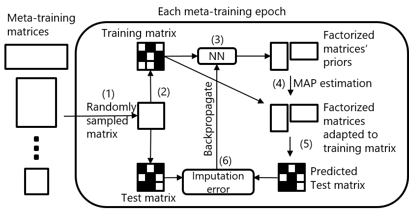
Figure 1: Our meta-learning framework: We are given multiple meta-training matrices. For each meta-training epoch, first, we generate a matrix from randomly selected rows and columns of a randomly selected matrix from the meta-training matrices. Second, we split elements in the matrix into training and test matrices. Third, factorized matrices’ priors are inferred by a neural network. Fourth, we adapt the factorized matrices to the training matrix by maximizing the posterior with a gradient descent method. Fifth, we impute the missing values by multiplying the adapted factorized matrices. Sixth, we calculate the missing value imputation error using the test matrix and backpropagate it to update neural network’s parameters.

The following are our major contributions:

1. We propose a meta-learning method for matrix imputation that can meta-learn from matrices without shared rows or columns.

2. We design a neural network to generate prior distributions of factorized matrices with different sizes, which is meta-trained such that the test matrix imputation performance improves when the factorized matrices are adapted to the training matrix based on the MAP estimation.

3. In our experiments using real-world data sets, we demonstrate that the proposed method achieves better matrix imputation performance when meta-training data contain matrices that are related to meta-test matrices.

2 Related work

Many meta-learning or few-shot learning methods have been proposed [43, 3, 38, 1, 51, 46, 2, 11, 34, 26, 12, 41, 56, 10, 13, 25, 18, 5, 39, 40]. These existing methods cannot learn from matrices without shared or and columns. With probabilistic meta-learning methods [12, 26], the prior of model parameters is meta-trained, where they require that the numbers of parameters are the same across tasks. Therefore, they are inapplicable for meta-learning nonparametric models, including matrix factorization, where the number of parameters can grow with the sample size. In contrast, the proposed method meta-trains a neural network that generates the prior of a task-specific model, which enables us to meta-learn nonparametric models. The proposed method is related to model-agnostic meta-learning [11] (MAML) in the sense that both methods backpropagate a loss through gradient descent steps. MAML learns the initial values of model parameters such that the performance improves when all the parameters are adapted to new tasks. The proposed method is more efficient than MAML since MAML requires a second-order gradient computation on the whole neural network while the proposed method requires that only on factorized matrices. In our model, we explicitly incorporate matrix factorization procedures by the gradient descent method, which has been successfully used for a wide variety of matrix imputation applications.

The proposed method is also related to encoder-decoder based meta-learning methods [53], such as neural processes [13]. The encoder-decoder based meta-learning methods obtain a representation of few observations by an encoder and use it in predictions by a decoder, where the encoder and decoder are modeled by neural networks. Similarly, the proposed method uses a neural network to obtain factorized matrices for predicting the missing values. Their differences are that the proposed method uses a neural network designed for matrices with missing values, and has gradient descent steps for adapting factorized matrices to observations. Adapting parameters by directly fitting them to observations is effective for meta-learning [32, 24] since it is difficult to output the adapted parameters only by neural networks for a wide variety of observations. The proposed method uses exchangeable matrix layers [17] as its components. The exchangeable matrix layers have not been used for meta-learning. Heterogeneous meta-learning [23] can learn from multiple tasks without shared attributes. However, it cannot handle missing values, and is inapplicable to matrix imputation.

Collective matrix factorization [45, 6, 55] simultaneously factorizes multiple matrices, where information in a matrix can be transferred to other matrices for factorization. Collective matrix factorization assumes that some of the columns and/or rows are shared across matrices. Transfer learning methods for matrix factorization that do not assume shared columns or rows have been proposed [22]. With such transfer learning methods, target matrices are required in the training phase for transferring knowledge from source to target matrices. On the other hand, the proposed method does not need to use target matrices for training. Several few-shot learning methods for recommender systems have been proposed [50, 33] to tackle the cold start problem, where the histories of new users or new items are insufficiently accumulated. These methods use auxiliary information, such as user attributes and item descriptions. In contrast, the proposed method does not use auxiliary information.

3 Proposed method

3.1 Problem formulation

Suppose that we are given $D$ matrices $\mathcal{X}=\{\mathbf{X}_{d}\}_{d=1}^{D}$ in the meta-training phase, where $\mathbf{X}_{d}\in\mathbb{R}^{N_{d}\times M_{d}}$ is the meta-training matrix in the $d$th task, and $x_{dnm}$ is its $(n,m)$th element. The sizes of the meta-training matrices can be different across tasks, $N_{d}\neq N_{d^{\prime}}$, $M_{d}\neq M_{d^{\prime}}$, and rows or columns are not shared across matrices. The meta-training matrices can contain missing values. In this case, we are additionally given binary indicator matrix $\mathbf{B}_{d}\in\{0,1\}^{N_{d}\times M_{d}}$, where $b_{dnm}=1$ if the $(n,m)$th element is observed, and $b_{dnm}=0$ otherwise. In the meta-test phase, we are given a meta-test matrix with missing values, $\mathbf{X}_{*}\in\mathbb{R}^{N_{*}\times M_{*}}$, where the missing values are specified by indicator matrix $\mathbf{B}_{*}\in\{0,1\}^{N_{*}\times M_{*}}$. Our aim is to improve the missing value imputation performance on the meta-test matrix.

3.2 Model

For each task, our model outputs factorized matrices $\mathbf{U}(\mathbf{X},\mathbf{B})\in\mathbb{R}^{N\times K}$ and $\mathbf{V}(\mathbf{X},\mathbf{B})\in\mathbb{R}^{M\times K}$ given matrix with missing values $\mathbf{X}\in\mathbb{R}^{N\times M}$ and its indicator matrix $\mathbf{B}\in\{0,1\}^{N\times M}$. In the meta-training phase, $\mathbf{X}$ and $\mathbf{B}$ are generated from one of meta-training matrices $\{\mathbf{X}_{d}\}_{d=1}^{D}$ as described in Section 3.3. In the meta-test phase, $\mathbf{X}$ and $\mathbf{B}$ correspond to meta-test matrix $\mathbf{X}_{*}$ and its indicator matrix $\mathbf{B}_{*}$. Figure 2 illustrates our model.

With our model, the factorized matrices are estimated by maximizing the posterior probability:

$$\mathbf{U}(\mathbf{X},\mathbf{B}),\mathbf{V}(\mathbf{X},\mathbf{B})=\arg\max_{\mathbf{U},\mathbf{V}}\left[\log p(\mathbf{X}|\mathbf{U},\mathbf{V})+\log p_{\mathbf{X}}(\mathbf{U},\mathbf{V}|\mathcal{X})\right],$$ (1)

where the first term is the likelihood,

$$\log p(\mathbf{X}|\mathbf{U},\mathbf{V})\propto-\sum_{n,m=1}^{N,M}b_{nm}(\mathbf{u}_{n}^{\top}\mathbf{v}_{m}-x_{nm})^{2},$$ (2)

the second term is the prior, $\mathbf{U}=[\mathbf{u}_{1},\cdots,\mathbf{u}_{N}]^{\top}$, $\mathbf{V}=[\mathbf{v}_{1},\cdots,\mathbf{v}_{M}]^{\top}$, and $\top$ is the transpose. We use subscript $\mathbf{X}$ in prior $p_{\mathbf{X}}$ to indicate that it is task-specific. The prior is conditioned on meta-training matrices $\mathcal{X}$ since we meta-learn it from $\mathcal{X}$. We assume a Gaussian prior with mean $\mathbf{u}_{n}^{(0)}$ ($\mathbf{v}_{m}^{(0)}$) and variance $\lambda^{-1}$:

$$\log p_{\mathbf{X}}(\mathbf{U},\mathbf{V}|\mathcal{X})\propto-\lambda\left(\sum_{n=1}^{N}\parallel\mathbf{u}_{n}-\mathbf{u}^{(0)}_{n}\parallel^{2}+\sum_{m=1}^{M}\parallel\mathbf{v}_{m}-\mathbf{v}^{(0)}_{m}\parallel^{2}\right).$$ (3)

We generate the task-specific prior mean values $\mathbf{u}_{n}^{(0)},\mathbf{v}_{m}^{(0)}$ with different sizes using a neural network. The neural network is shared across different tasks, which enables us to extract knowledge in the meta-training matrices, and use the knowledge for unseen tasks. When $\lambda=0$, matrix factorization is independently performed for each matrix, and it cannot meta-learn useful knowledge for factorization.

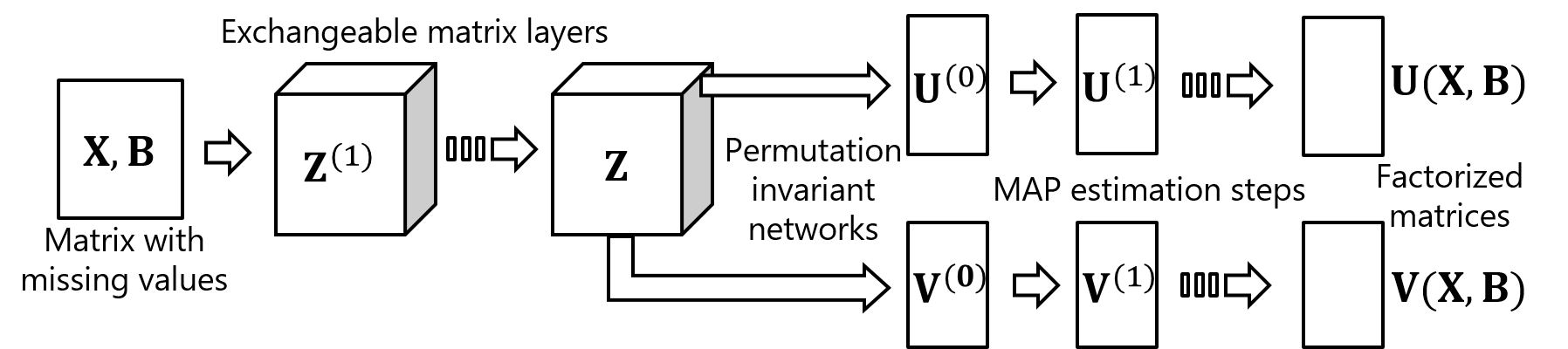
Figure 2: Our model: Matrix with missing values $\mathbf{X}$ and its indicator matrix $\mathbf{B}$ are the input. First, representations $\mathbf{Z}$ for each element in $\mathbf{X}$ are obtained by exchangeable matrix layers in Eq. (4). Second, the mean of the prior of factorized matrices $\mathbf{U}^{(0)}$ and $\mathbf{V}^{(0)}$ is calculated by transforming the averages of representations $\mathbf{Z}$ over columns and rows by permutation invariant neural networks in Eq. (5). Third, factorized matrices $\mathbf{U}(\mathbf{X},\mathbf{B})$ and $\mathbf{V}(\mathbf{X},\mathbf{B})$ are estimated by maximizing the posterior probability using the gradient descent steps in Eqs. (6,7). For each gradient descent step, input $\mathbf{X}$ and $\mathbf{B}$ and prior means $\mathbf{U}^{(0)}$ and $\mathbf{V}^{(0)}$ are used as well as previous estimates $\mathbf{U}^{(t-1)}$ and $\mathbf{V}^{(t-1)}$. Our model can take matrices with different sizes as input, and output their factorized matrices.

For modeling the prior, first, we obtain representations $\mathbf{Z}\in\mathbb{R}^{N\times M\times C}$ of given matrix $\mathbf{X}$ using a neural network, where the matrix’s $(n,m)$th element is represented by vector $\mathbf{z}_{nm}\in\mathbb{R}^{C}$. Our model uses exchangeable matrix layers [17]:

$$z^{(\ell+1)}_{nmc} =\sigma\Biggl{(}\sum_{c^{\prime}=1}^{C^{(\ell)}}\Bigl{(}w_{c^{\prime}c1}^{(\ell)}b_{nm}z_{nmc^{\prime}}^{(\ell)}+w_{c^{\prime}c2}^{(\ell)}\frac{\sum_{n^{\prime}=1}^{N}b_{n^{\prime}m}z_{n^{\prime}mc^{\prime}}^{(\ell)}}{\sum_{n^{\prime}=1}^{N}b_{n^{\prime}m}}+w_{c^{\prime}c3}^{(\ell)}\frac{\sum_{m^{\prime}=1}^{M}b_{nm^{\prime}}z_{nm^{\prime}c^{\prime}}^{(\ell)}}{\sum_{m^{\prime}=1}^{M}b_{nm^{\prime}}}$$

$$+w_{c^{\prime}c4}^{(\ell)}\frac{\sum_{n^{\prime},m^{\prime}=1}^{N,M}b_{n^{\prime}m^{\prime}}z_{n^{\prime}m^{\prime}c^{\prime}}^{(\ell)}}{\sum_{n^{\prime},m^{\prime}=1}^{N,M}b_{n^{\prime}m^{\prime}}}+w_{c5}^{(\ell)}\Bigr{)}\Biggr{)},$$ (4)

where $z^{(\ell)}_{nmc}\in\mathbb{R}$ is the $c$th channel of the representation of the $(n,m)$ element in the $\ell$th layer, $w_{c^{\prime}ci}^{(\ell)}\in\mathbb{R}$ is a weight parameter in the $\ell$th layer to be trained for the influence of channel $c^{\prime}$ on channel $c$ in the next layer, $\sigma$ is an activation function, and $C^{(\ell)}$ is the channel size of the $\ell$th layer. In the first layer, the given matrix is used for representation $\mathbf{z}^{(0)}_{nm}=x_{nm}\in\mathbb{R}$, where $x_{nm}$ is the value of the $(n,m)$ element of given matrix $\mathbf{X}$. The representation in the last layer is used as final representation $\mathbf{Z}=\mathbf{Z}^{(L)}$, where $L$ is the number of layers, and $C^{(L)}=C$. In the last layer, activation function $\sigma$ is omitted. The first term in Eq. (4) calculates the influence from the same element, the second term calculates the influence from the elements of the same column, the third term calculates the influence from the elements of the same row, the fourth term calculates the influence from all the elements, and the fifth term is the bias. The influences are averaged over the observed elements using indicator matrix $\mathbf{B}$. The exchangeable matrix layer is permutation equivariant, where the output is the same values across all the row- and column-wise permutations of the input. With the exchangeable matrix layers, we can obtain representations for each element considering the whole matrix. The exchangeable matrix layers can handle matrices with different sizes since their parameters $w^{(\ell)}_{c^{\prime}ci}$ do not depend on the input matrix size.

Second, we calculate the mean of the priors of the factorized matrices using permutation invariant networks [57]:

$$\mathbf{u}^{(0)}_{n}=f_{\mathrm{U}}\left(\frac{1}{M}\sum_{m=1}^{M}\mathbf{z}_{nm}\right),\quad\mathbf{v}^{(0)}_{m}=f_{\mathrm{V}}\left(\frac{1}{N}\sum_{n=1}^{N}\mathbf{z}_{nm}\right),$$ (5)

where $\mathbf{u}^{(0)}_{n}\in\mathbb{R}^{K}$ is the prior mean of the $n$th row of factorized matrix $\mathbf{U}$, $\mathbf{v}^{(0)}_{m}\in\mathbb{R}^{K}$ is the pror mean of the $m$th row of factorized matrix $\mathbf{V}$, and $f_{\mathrm{U}}$ and $f_{\mathrm{V}}$ are feed-forward neural networks. In Eq. (5), we take the average of element representation $\mathbf{Z}$ over the rows (columns) and input them into the neural networks. Eq. (5) is a permutation invariant operation that can take any number of elements $N$ and $M$. By Eqs. (4,5), we can obtain prior mean values $\mathbf{u}^{(0)}_{n}$ and $\mathbf{v}^{(0)}_{m}$ for each row and column considering the relationship with other elements in the given matrix. Parameters $\{w_{c^{\prime}ci}^{(\ell)}\}$ and parameters in $f_{\mathrm{U}}$, $f_{\mathrm{V}}$ are common for all matrices. Prior mean values $\mathbf{U}^{(0)}$, $\mathbf{V}^{(0)}$ are different across matrices since they are calculated from input matrices $\mathbf{X}$ and $\mathbf{B}$.

We estimate the factorized matrices by the MAP estimation in Eq. (1) using the prior mean values in Eq. (5) as the initial values. The update rules of the MAP estimation based on the gradient descent method are given in a closed form by taking the gradient of the objective function with respect to factorized matrices $\mathbf{u}_{n}$ and $\mathbf{v}_{m}$:

$$\mathbf{u}^{(t+1)}_{n}=\mathbf{u}^{(t)}_{n}-\eta\Bigl{(}\sum_{m=1}^{M}b_{nm}(\mathbf{u}_{n}^{(t)\top}\mathbf{v}^{(t)}_{m}-x_{nm})\mathbf{v}^{(t)}_{m}+\lambda(\mathbf{u}^{(t)}_{n}-\mathbf{u}^{(0)}_{n})\Bigr{)},$$ (6)

$$\mathbf{v}^{(t+1)}_{m}=\mathbf{v}^{(t)}_{m}-\eta\Bigl{(}\sum_{n=1}^{N}b_{nm}(\mathbf{u}_{n}^{(t)\top}\mathbf{v}^{(t)}_{m}-x_{nm})\mathbf{u}^{(t)}_{n}+\lambda(\mathbf{v}^{(t)}_{m}-\mathbf{v}^{(0)}_{m})\Bigr{)},$$ (7)

where $\mathbf{u}^{(t)}$ and $\mathbf{v}^{(t)}$ are estimated factorized matrices at the $t$th iteration, and $\eta>0$ is the learning rate. The factorized matrices at the $T$th iteration are used as the output of our model $\mathbf{U}(\mathbf{X},\mathbf{B})=\mathbf{U}^{(T)}$, $\mathbf{V}(\mathbf{X},\mathbf{B})=\mathbf{V}^{(T)}$. The missing value in $\mathbf{X}$ is predicted by the inner product of the factorized matrices by

$$\hat{x}_{nm}=\mathbf{u}_{n}(\mathbf{X},\mathbf{B})^{\top}\mathbf{v}_{m}(\mathbf{X},\mathbf{B}).$$ (8)

We could predict the missing values using the output of the neural networks, $\hat{x}_{nm}=\mathbf{u}_{n}^{(0)\top}\mathbf{v}_{m}^{(0)}$, without the gradient descent steps. However, the prediction might be different from the true values even with the observed elements if the given matrix does not resemble any of the meta-training matrices that are used for optimizing the neural networks, and the generalization performance of the neural networks is not high enough. With gradient descent steps, the factorized matrices can be adapted to the given matrix even when the neural networks fail to adapt. Minimizing the error between the observed and predicted values is a standard technique for matrix factorization [29]. We use it as a component in our model.

Our model can be seen as a single neural network, that takes a matrix with missing values as input, and outputs its factorized matrices, where the exchangeable matrix layers in Eq. (4), the permutation invariant networks in Eq. (5), and the gradient descent steps in Eqs. (6,7) are used as layers (Figure 2). Algorithm 1 shows the forwarding procedures of our model. Since our model including the gradient descent steps is differentiable, we can backpropagate the loss through the gradient descent steps to update the parameters in our neural networks.

Algorithm 1 Forwarding procedures of our model.

0:  Observed matrix with missing values $\mathbf{X}$, indicator matrix $\mathbf{B}$, number of iterations $T$

0:  Factorized matrices $\mathbf{U}(\mathbf{X},\mathbf{B})$, $\mathbf{V}(\mathbf{X},\mathbf{B})$

1:  Obtain element representations $\mathbf{Z}$ by Eq. (4).

2:  Calculate the mean of the priors of factorized matrices $\mathbf{U}^{(0)}$ and $\mathbf{V}^{(0)}$ by Eq. (5).

3:  for $t:=1$ to $T$ do

4:     Update factorized matrices $\mathbf{U}^{(t)}$, $\mathbf{V}^{(t)}$ by Eqs. (6,7) based on the MAP estimation.

5:  end for

3.3 Meta-training

We meta-train model parameters $\bm{\Theta}$, i.e., exchangeable matrix layer parameters $\{\{\{\{\{w^{(\ell)}_{cc^{\prime}i}\}_{i=1}^{5}\}_{c^{\prime}=1}^{C^{\ell}}\}_{c=1}^{C^{\ell+1}}\}_{\ell=1}^{L-1}$, the parameters of feed-forward neural networks $f_{\mathrm{U}}$ and $f_{\mathrm{V}}$, and regularization parameter $\lambda$, by minimizing the following expected test error of the missing values with the episodic training framework:

$$\mathbb{E}_{\mathbf{X},\mathbf{B},\mathbf{X}^{\prime},\mathbf{B}^{\prime}}[\parallel\mathbf{B}^{\prime}\odot(\mathbf{X}^{\prime}-\mathbf{U}(\mathbf{X},\mathbf{B})^{\top}\mathbf{V}(\mathbf{X},\mathbf{B}))\parallel^{2}],$$ (9)

where $\mathbf{X}$ and $\mathbf{X}^{\prime}$ are sampled training and test matrices, $\mathbf{B}$ and $\mathbf{B}^{\prime}$ are their indicator matrices, $\mathbf{U}(\mathbf{X},\mathbf{B})\in\mathbb{R}^{N\times K}$ and $\mathbf{V}(\mathbf{X},\mathbf{B})\in\mathbb{R}^{M\times K}$ are the factorized matrices obtained by our model from training matrix $\mathbf{X}$ and its indicator matrix $\mathbf{B}$, $\mathbb{E}$ is the expectation, and $\odot$ is the element-wise multiplication. Eq. (9) is the expectation error between the test matrix and its imputation by our model adapted to the training matrix.

Algorithm 2 shows the meta-training procedures of our model. In Line 4, matrix $\bar{\mathbf{X}}\in\mathbb{R}^{N\times M}$ is constructed from randomly selected meta-training matrix $\mathbf{X}_{d}$, where $\bar{\mathbf{X}}$ is a submatrix of $\mathbf{X}_{d}$. Instead of sampling the submatrices, we can use the whole selected meta-training matrix $\bar{\mathbf{X}}=\mathbf{X}_{d}$, or change the number of rows and columns, $N$ and $M$, for each epoch. In Line 5, the non-missing elements in matrix $\bar{\mathbf{X}}$ are randomly split into training matrix $\mathbf{X}$ and test matrix $\mathbf{X}^{\prime}$, where their indicator matrices are mutually exclusive, $\mathbf{B}\cap\mathbf{B}^{\prime}=\phi$. We assume that the meta-test matrices are missing at random. If they are missing not at random, we can model missing patterns [35], and use them for generating training and test matrices in the meta-training procedures.

The time complexity for each meta-training step is $O(\gamma LNM+T(\gamma NM+(N+M)K)+\gamma^{\prime}NM)$, where $\gamma$ is the rate of the observed elements in a training matrix, and $\gamma^{\prime}$ is that in a test matrix. The first term $O(\gamma LNM)$ is for inferring the priors by the neural networks. The second term $O(T(\gamma NM+(N+M)K))$ is for the MAP estimation of the factorized matrices using Eqs. (6,7). The third term $O(\gamma^{\prime}NM)$ is for calculating the loss on the test matrix. The number of model parameters $\bm{\Theta}$ depends on neither the meta-training data size nor the numbers of rows $N$ and columns $M$ of the training and test matrices.

Algorithm 2 Meta-training procedure of our model.

0:  Meta-training data $\{\mathbf{X}_{d}\}_{d=1}^{D}$, number of rows $N$, number of columns $M$, training ratio $R$, number of iterations $T$

0:  Trained model parameters $\bm{\Theta}$

1:  Initialize model parameters $\bm{\Theta}$.

2:  while End condition is satisfied do

3:     Randomly select task index $d$ from $\{1,\cdots,D\}$.

4:     Randomly sample $N$ rows and $M$ columns from $\mathbf{X}_{d}$ and construct matrix $\bar{\mathbf{X}}$.

5:     Randomly assign non-missing elements in $\bar{\mathbf{X}}$ with probability $R$ as training matrix $\mathbf{X}$, and assign the remaining non-missing elements as test matrix $\mathbf{X}^{\prime}$.

6:     Obtain factorized matrices $\mathbf{U}(\mathbf{X},\mathbf{B}),\mathbf{V}(\mathbf{X},\mathbf{B})$ of the training matrix by Algorithm 1.

7:     Calculate loss $\parallel\mathbf{B}^{\prime}\odot(\mathbf{X}^{\prime}-\mathbf{U}(\mathbf{X},\mathbf{B})^{\top}\mathbf{V}(\mathbf{X},\mathbf{B}))\parallel^{2}$ on the test matrix and its gradient.

8:     Update model parameters $\bm{\Theta}$ using the loss and gradient by a stochastic gradient method.

9:  end while

4 Experiments

4.1 Data

We evaluated the proposed method using three rating datasets: ML100K, ML1M [15], and Jester [14] . The ML100K data contained 100,000 ratings of 1,682 movies by 943 users. The ML1M data contained 1,000,209 ratings of 3,952 movies by 6,040 users. The Jester data contained 1,805,072 ratings of 100 jokes from 24,983 users. The ratings of each dataset were normalized with zero mean and unit variance. We randomly split the users and items, and used 70% of them for meta-training, 10% for meta-validation, and the remaining for meta-test. There were no overlaps of users and items across the meta-training, validation, and test data. We randomly generated ten $30\times 30$ meta-test matrices from the meta-test data and used half of the originally observed ratings as missing ratings for evaluation. For each meta-test matrix, the average numbers of observed elements were respectively 28.8, 19.0, and 218.0 in the ML100K, ML1M, and Jester data. We did not use the meta-test matrices in the meta-training phase. The evaluation measurement was the test mean squared error, which was calculated by the mean squared error between the true and estimated ratings of the unobserved elements in the meta-test matrices. We averaged the test mean squared errors over ten experiments with different splits of meta-training, validation, and test data.

4.2 Proposed method setting

We used three exchangeable matrix layers with 32 channels. Feed-forward neural networks $f_{\mathrm{u}},f_{\mathrm{v}}$ were four-layered with 32 hidden units and $K=32$ output units. We used a rectified linear unit, $\mathrm{ReLU}(x)=\max(0,x)$, for the activation. For the gradient descent steps of the matrix factorization in Eqs. (6,7), the learning rate was $\eta=10^{-2}$, and the number of iterations was $T=10$. The number of rows and columns of the training matrices were $N=30$ and $M=30$, and the training ratio was $R=0.5$. We optimized our model using Adam [28] with learning rate $10^{-4}$, batch size $16$, and dropout rate $0.1$ [47]. The number of meta-training epochs was 1,000, and the meta-validation data were used for early stopping. We implemented the proposed method with PyTorch [37].

4.3 Comparing methods

We compared the proposed method with the following eight methods: exchangeable matrix layer neural networks (EML) [17], EML finetuned with the meta-test matrix (FT), model-agnostic meta-learning of EML (MAML) [11], item-based AutoRec (AutoRecI) [44], user-based AutoRec (AutoRecU), deep matrix factorization (DMF) [54], matrix factorization (MF), and the mean value of the meta-test matrix (Mean). EML, FT, MAML as well as the proposed method were meta-learning schemes, all of which were trained using the meta-training matrices such that the test mean squared error was minimized. AutoRecI, AutoRecU, DMF, MF, and Mean were trained using the observed ratings of the meta-test matrix by minimizing the mean squared error without meta-training matrices.

EML used three exchangeable matrix layers, where the number of channels with the first two layers was 32, and the number of channels with the last layer was one to output the estimation of a rating. EML was trained with the episodic framework like the proposed method. The exchangeable matrix layers have not been used for meta-learning. We newly used them for meta-learning by employing them as the encoder and decoder in an encoder-decoder based meta-learning method. FT finetuned the parameters of the trained EML using the observed ratings in the meta-test matrix by minimizing the mean squared error. MAML trained the initial parameters of EML to minimize the test mean squared error when finetuned by the episodic training framework. The number of iterations in the inner loop was five. AutoRec is a neural network-based matrix imputation method. With AutoRecI (AutoRecU), a neural network took each row (column) as input and output its reconstruction. DMF is a neural network-based matrix factorization method, where the row and column representations were calculated by neural networks that took a row or column as input, and ratings were estimated by the inner product of the row and column representations. For the neural networks in AutoRecI, AutoRecU, and DMF, we used four-layered feed-forward neural networks with 32 hidden units. With DMF and MF, the number of latent factors was 32. With AutoRecI, AutoRecU, DMF, and MF, the weight decay parameter was tuned from $\{10^{-4},10^{-3},10^{-2},10^{-1},1\}$, and the learning rate was tuned from $\{10^{-3},10^{-2},10^{-1}\}$ using the validation data.

4.4 Results

Table 1: Average test mean squared errors on unobserved elements in test matrices and their standard error: Values in bold are not statistically different at 5% level from the best performing method in each dataset by a paired t-test.

	ML100K	ML1M	Jester
Ours	0.901 $\pm$ 0.033	0.883 $\pm$ 0.024	0.813 $\pm$ 0.009
EML	0.933 $\pm$ 0.036	0.907 $\pm$ 0.024	0.848 $\pm$ 0.009
FT	1.175 $\pm$ 0.047	1.149 $\pm$ 0.046	0.990 $\pm$ 0.008
MAML	0.941 $\pm$ 0.036	0.904 $\pm$ 0.025	0.880 $\pm$ 0.011
AutoRecI	0.985 $\pm$ 0.040	0.968 $\pm$ 0.028	0.949 $\pm$ 0.008
AutoRecU	0.987 $\pm$ 0.033	0.962 $\pm$ 0.024	0.907 $\pm$ 0.014
DMF	0.979 $\pm$ 0.034	0.972 $\pm$ 0.023	0.852 $\pm$ 0.007
MF	1.014 $\pm$ 0.037	0.962 $\pm$ 0.031	1.005 $\pm$ 0.014
Mean	1.007 $\pm$ 0.020	0.983 $\pm$ 0.013	1.004 $\pm$ 0.008

(a) ML100K	(b) ML1M	(c) Jester

Figure 3: Average test mean squared errors when meta-trained with training and test matrices of different sizes, where the size of the meta-test matrices was the same as that of the training and test matrices. We used square matrices, and the horizontal axis is the number of columns and rows. Bar show the standard error.

(a) ML100K	(b) ML1M	(c) Jester

Figure 4: Average test mean squared errors with meta-test matrices with different sizes, where the model was meta-trained with $30\times 30$ matrices. We used square matrices, and the horizontal axis is the number of columns and rows. Bars show the standard error.

Table 1 shows the average test mean squared error. The proposed method achieved the lowest error on all the datasets. EML’s performance was the second best on the ML100K and Jester datasets. This result indicates that exchangeable matrix layers effectively extracted useful information from the matrices with missing values. The proposed method further improved the performance from EML by directly adapting to the observed elements using the gradient descent steps based on MAP estimation. Since EML approximates the adaptation to the observed elements only by exchangeable matrix layers, the estimated values can be different from the observed elements. The errors on the observed elements with EML were higher than those with the proposed method shown in the supplementary material. With FT, although the errors on the observed elements were low, the test errors on the unobserved elements were high, because FT was overfitted to the observed values by training the model by minimizing the error on the observed elements. On the other hand, the proposed method trains the model by minimizing the test error on the unobserved elements when fitted to the observed elements with MAP estimation. Therefore, the proposed method alleviated overfitting to the observed elements. Since MAML trained the model by minimizing the expected test error, the overfitting was smaller than FT. However, MAML’s performance did not surpass that of EML and was lower than that of the proposed method. With MAML, the whole neural network-based model is adapted to the observed values. In contrast, the proposed method adapts only factorized matrices to the observed values, although the neural networks are fixed and used for defining the priors of the factorized matrices. The errors of the methods that did not use meta-training matrices, i.e., AutoRec, DMF, MF, and Mean, were high since they needed to estimate the missing values only from a small number of observations. On the other hand, the proposed method achieved the lowest error by meta-learning hidden structure in the meta-training matrices that effectively improved the test matrix imputation performance even though rows and columns were not shared across different matrices.

Figure 3 shows the test mean squared errors when meta-trained with training and test matrices of different sizes, where the size of the meta-test matrices was the same as that of the training and test matrices. Our proposed method and EML decreased the error as the matrix size increased because the number of observations rose as the matrix size increased. Figure 4 shows the test mean squared errors with meta-test matrices of different sizes, where the model was meta-trained with $30\times 30$ matrices. The proposed method achieved the lowest error with different sizes of meta-test matrices. The proposed method’s performance improved as the meta-test matrix size increased even though it was trained with different-sized matrices.

Figure 5 shows the test mean squared errors with different numbers of gradient descent iterations with the proposed method. As the number of iterations increased, the error decreased especially with the ML100K and Jester data. This result indicates the effectiveness of the gradient descent steps in the proposed method.

(a) ML100K	(b) ML1M	(c) Jester

Figure 5: Average test mean squared errors with different numbers of gradient descent iterations with the proposed method. Bar show the standard error.

Table 2 shows the average training mean squared errors. The errors on the observed elements with EML were higher than those with the proposed method.

Table 3 shows the average test mean squared errors by the proposed method when different datasets were used between meta-training and meta-test data. With the ML1M and Jester meta-test data, the proposed method achieved the best performance when meta-trained with matrices from the same dataset. Even when the meta-training datasets were different from the meta-test datasets, the errors were relatively low, and they were lower than those by the comparing methods. This is because the datasets used in our experiments were related to each other and shared some hidden structure, and the proposed method learned the shared structure and used the learned structure to improve the matrix imputation performance in the other datasets.

Table 4 shows the average test mean squared errors by the proposed method with different factorized matrix ranks $K$. The proposed method worked even when factorized matrix rank $K$ is larger than the number of rows $N$ or columns $M$ since it uses the priors inferred by the neural networks based on the MAP estimation. Factorized matrix rank $K$ slightly affects the performance, but the proposed method achieved better performance than the comparing methods with a wide range of $K$.

Table 5 shows the average test mean squared errors by AutoRec with different numbers of hidden units. With any numbers of hidden units, the performance by AutoRec was worse than the proposed method.

Tables 6 and 7 show the computational time in seconds for meta-training and test on computers with 2.60GHz CPUs. The meta-training time of the proposed method was much shorter than MAML since the proposed method adapts only factorized matrices instead of neural networks, where the adaption steps can be written explicitly. The meta-training time of the proposed method was longer than EML since the proposed method additionally requires adaptation steps. The proposed method’s meta-test time was short since it requires only a small number of adaptation steps for a few observed elements.

Table 2: Average mean squared errors on observed elements in test matrices and their standard error with meta-learning methods.

	ML100K	ML1M	Jester
Ours	0.504 $\pm$ 0.017	0.354 $\pm$ 0.013	0.618 $\pm$ 0.008
EML	0.596 $\pm$ 0.018	1.573 $\pm$ 0.071	0.664 $\pm$ 0.010
FT	0.328 $\pm$ 0.013	0.346 $\pm$ 0.017	0.528 $\pm$ 0.012
MAML	0.493 $\pm$ 0.012	0.503 $\pm$ 0.028	0.658 $\pm$ 0.013

Table 3: Average test mean squared errors by the proposed method with different pairs of meta-training and meta-test datasets. Each row represents the meta-training data, and each column represents the meta-test data.

Meta-training data $\backslash$ Meta-test data	ML100K	ML1M	Jester
ML100K	0.901 $\pm$ 0.033	0.906 $\pm$ 0.023	0.825 $\pm$ 0.008
ML1M	0.889 $\pm$ 0.028	0.883 $\pm$ 0.024	0.827 $\pm$ 0.008
Jester	0.900 $\pm$ 0.027	0.927 $\pm$ 0.025	0.813 $\pm$ 0.009
ML100K, ML1M	0.894 $\pm$ 0.036	0.883 $\pm$ 0.024	0.829 $\pm$ 0.008
ML100K, Jester	0.894 $\pm$ 0.031	0.893 $\pm$ 0.025	0.824 $\pm$ 0.008
ML1M, Jester	0.884 $\pm$ 0.035	0.885 $\pm$ 0.024	0.832 $\pm$ 0.008
ML100K, ML1M, Jester	0.892 $\pm$ 0.035	0.884 $\pm$ 0.023	0.829 $\pm$ 0.008

Table 4: Average test mean squared errors by the proposed method with different factorized matrix ranks $K$.

$K$	8	16	32	64	128
ML100K	0.908	0.903	0.901	0.899	0.898
ML1M	0.889	0.887	0.883	0.888	0.886
Jester	0.815	0.814	0.813	0.814	0.813

Table 5: Average test mean squared errors by AutoRec with different numbers of hidden units.

	AutoRecI		AutoRecU
#hidden units	128	512	128	512
ML100K	0.980	0.974	0.998	0.979
ML1M	0.949	0.954	0.946	0.947
Jester	0.924	0.929	0.876	0.917

Table 6: Meta-training time in seconds.

	ML100K	ML1M	Jester
Ours	1039	3527	376
EML	850	2983	247
MAML	15983	55205	4189

Table 7: Meta-test time in seconds.

	ML100K	ML1M	Jester
Ours	0.13	0.13	0.14
EML	0.09	0.09	0.10
FT	3.88	3.75	2.77
MAML	1.72	3.12	1.60
AutoRecI	1.51	1.54	3.60
AutoRecU	1.50	1.49	3.99
DMF	1.78	5.20	4.49
MF	0.53	1.20	1.29

5 Conclusion

We proposed a neural network-based meta-learning method for matrix imputation that learns from multiple matrices without shared rows and columns, and predicts the missing values given observations in unseen matrices. Although we believe that our work is an important step for learning from a wide variety of matrices, we must extend our approach in several directions. First, we will apply our framework to tensor data using exchangeable tensor layers [17] and tensor factorizations [19, 8, 16, 49, 52, 30]. Second, we will use our framework for other types of matrix factorization, such as non-negative matrix factorization (NMF) [31] and independent component analysis [21]. For example, we can use multiplicative update steps for NMF instead of gradient descent steps. Third, we want to extend our proposed method to use auxiliary information, e.g., user and item information in recommender systems, by taking it as input of our neural network.

References

- [1] M. Andrychowicz, M. Denil, S. Gomez, M. W. Hoffman, D. Pfau, T. Schaul, B. Shillingford, and N. De Freitas. Learning to learn by gradient descent by gradient descent. In Advances in Neural Information Processing Systems, pages 3981–3989, 2016.
- [2] S. Bartunov and D. Vetrov. Few-shot generative modelling with generative matching networks. In International Conference on Artificial Intelligence and Statistics, pages 670–678, 2018.
- [3] Y. Bengio, S. Bengio, and J. Cloutier. Learning a synaptic learning rule. In International Joint Conference on Neural Networks, 1991.
- [4] D. Bokde, S. Girase, and D. Mukhopadhyay. Matrix factorization model in collaborative filtering algorithms: A survey. Procedia Computer Science, 49:136–146, 2015.
- [5] J. Bornschein, A. Mnih, D. Zoran, and D. J. Rezende. Variational memory addressing in generative models. In Advances in Neural Information Processing Systems, pages 3920–3929, 2017.
- [6] G. Bouchard, D. Yin, and S. Guo. Convex collective matrix factorization. In Artificial Intelligence and Statistics, pages 144–152, 2013.
- [7] J.-P. Brunet, P. Tamayo, T. R. Golub, and J. P. Mesirov. Metagenes and molecular pattern discovery using matrix factorization. Proceedings of the National Academy of Sciences, 101(12):4164–4169, 2004.
- [8] J. D. Carroll and J.-J. Chang. Analysis of individual differences in multidimensional scaling via an n-way generalization of eckart-young decomposition. Psychometrika, 35(3):283–319, 1970.
- [9] S. T. Dumais. Latent semantic analysis. Annual review of information science and technology, 38(1):188–230, 2004.
- [10] H. Edwards and A. Storkey. Towards a neural statistician. arXiv preprint arXiv:1606.02185, 2016.
- [11] C. Finn, P. Abbeel, and S. Levine. Model-agnostic meta-learning for fast adaptation of deep networks. In Proceedings of the 34th International Conference on Machine Learning, pages 1126–1135, 2017.
- [12] C. Finn, K. Xu, and S. Levine. Probabilistic model-agnostic meta-learning. In Advances in Neural Information Processing Systems, pages 9516–9527, 2018.
- [13] M. Garnelo, D. Rosenbaum, C. Maddison, T. Ramalho, D. Saxton, M. Shanahan, Y. W. Teh, D. Rezende, and S. A. Eslami. Conditional neural processes. In International Conference on Machine Learning, pages 1690–1699, 2018.
- [14] K. Goldberg, T. Roeder, D. Gupta, and C. Perkins. Eigentaste: A constant time collaborative filtering algorithm. information retrieval, 4(2):133–151, 2001.
- [15] F. M. Harper and J. A. Konstan. The Movielens datasets: History and context. ACM Transactions on Interactive Intellgigent Systems, 5(4):1–19, 2015.
- [16] R. HARSHMAN. Foundations of the PARAFAC procedure: Models and conditions for an" explanatory" multi-mode factor analysis. UCLA Working Papers in Phonetics, 16:1–84, 1970.
- [17] J. Hartford, D. Graham, K. Leyton-Brown, and S. Ravanbakhsh. Deep models of interactions across sets. In International Conference on Machine Learning, pages 1909–1918, 2018.
- [18] L. B. Hewitt, M. I. Nye, A. Gane, T. Jaakkola, and J. B. Tenenbaum. The variational homoencoder: Learning to learn high capacity generative models from few examples. arXiv preprint arXiv:1807.08919, 2018.
- [19] F. L. Hitchcock. The expression of a tensor or a polyadic as a sum of products. Journal of Mathematics and Physics, 6(1-4):164–189, 1927.
- [20] T. Hofmann. Unsupervised learning by probabilistic latent semantic analysis. Machine learning, 42(1-2):177–196, 2001.
- [21] A. Hyvärinen and E. Oja. Independent component analysis: algorithms and applications. Neural networks, 13(4-5):411–430, 2000.
- [22] T. Iwata and T. Koh. Cross-domain recommendation without shared users or items by sharing latent vector distributions. In Artificial Intelligence and Statistics, pages 379–387, 2015.
- [23] T. Iwata and A. Kumagai. Meta-learning from tasks with heterogeneous attribute spaces. In Advances in Neural Information Processing Systems, 2020.
- [24] T. Iwata and Y. Tanaka. Few-shot learning for spatial regression. arXiv preprint arXiv:2010.04360, 2020.
- [25] H. Kim, A. Mnih, J. Schwarz, M. Garnelo, A. Eslami, D. Rosenbaum, O. Vinyals, and Y. W. Teh. Attentive neural processes. In International Conference on Learning Representations, 2019.
- [26] T. Kim, J. Yoon, O. Dia, S. Kim, Y. Bengio, and S. Ahn. Bayesian model-agnostic meta-learning. In Advances in Neural Information Processing Systems, 2018.
- [27] T. Kimura, K. Ishibashi, T. Mori, H. Sawada, T. Toyono, K. Nishimatsu, A. Watanabe, A. Shimoda, and K. Shiomoto. Spatio-temporal factorization of log data for understanding network events. In IEEE Conference on Computer Communications, pages 610–618. IEEE, 2014.
- [28] D. P. Kingma and J. Ba. Adam: A method for stochastic optimization. In International Conference on Learning Representations, 2015.
- [29] Y. Koren, R. Bell, and C. Volinsky. Matrix factorization techniques for recommender systems. Computer, 42(8):30–37, 2009.
- [30] V. Kuleshov, A. Chaganty, and P. Liang. Tensor factorization via matrix factorization. In Artificial Intelligence and Statistics, pages 507–516, 2015.
- [31] D. D. Lee and H. S. Seung. Learning the parts of objects by non-negative matrix factorization. Nature, 401(6755):788–791, 1999.
- [32] K. Lee, S. Maji, A. Ravichandran, and S. Soatto. Meta-learning with differentiable convex optimization. In Proceedings of the IEEE Conference on Computer Vision and Pattern Recognition, pages 10657–10665, 2019.
- [33] R. Li, X. Wu, X. Wu, and W. Wang. Few-shot learning for new user recommendation in location-based social networks. In Proceedings of The Web Conference, pages 2472–2478, 2020.
- [34] Z. Li, F. Zhou, F. Chen, and H. Li. Meta-SGD: Learning to learn quickly for few-shot learning. arXiv preprint arXiv:1707.09835, 2017.
- [35] B. Marlin, R. S. Zemel, S. Roweis, and M. Slaney. Collaborative filtering and the missing at random assumption. In Proceedings of the Conference on Uncertainty in Artificial Intelligence, pages 267–275, 2007.
- [36] A. Mnih and R. R. Salakhutdinov. Probabilistic matrix factorization. In Advances in Neural Information Processing Systems, pages 1257–1264, 2008.
- [37] A. Paszke, S. Gross, S. Chintala, G. Chanan, E. Yang, Z. DeVito, Z. Lin, A. Desmaison, L. Antiga, and A. Lerer. Automatic differentiation in PyTorch. In NIPS Autodiff Workshop, 2017.
- [38] S. Ravi and H. Larochelle. Optimization as a model for few-shot learning. In International Conference on Learning Representations, 2017.
- [39] S. Reed, Y. Chen, T. Paine, A. v. d. Oord, S. Eslami, D. Rezende, O. Vinyals, and N. de Freitas. Few-shot autoregressive density estimation: Towards learning to learn distributions. arXiv preprint arXiv:1710.10304, 2017.
- [40] D. J. Rezende, S. Mohamed, I. Danihelka, K. Gregor, and D. Wierstra. One-shot generalization in deep generative models. In Proceedings of the 33rd International Conference on International Conference on Machine Learning, pages 1521–1529, 2016.
- [41] A. A. Rusu, D. Rao, J. Sygnowski, O. Vinyals, R. Pascanu, S. Osindero, and R. Hadsell. Meta-learning with latent embedding optimization. In International Conference on Learning Representations, 2019.
- [42] R. Salakhutdinov and A. Mnih. Bayesian probabilistic matrix factorization using mcmc. In International Conference in Machine Learning, pages 872–879, 2008.
- [43] J. Schmidhuber. Evolutionary principles in self-referential learning. on learning now to learn: The meta-meta-meta…-hook. Master’s thesis, Technische Universitat Munchen, Germany, 1987.
- [44] S. Sedhain, A. K. Menon, S. Sanner, and L. Xie. AutoRec: Autoencoders meet collaborative filtering. In Proceedings of the 24th International Conference on World Wide Web, pages 111–112, 2015.
- [45] A. P. Singh and G. J. Gordon. Relational learning via collective matrix factorization. In Proceedings of the 14th ACM SIGKDD international conference on Knowledge discovery and data mining, pages 650–658, 2008.
- [46] J. Snell, K. Swersky, and R. Zemel. Prototypical networks for few-shot learning. In Advances in Neural Information Processing Systems, pages 4077–4087, 2017.
- [47] N. Srivastava, G. Hinton, A. Krizhevsky, I. Sutskever, and R. Salakhutdinov. Dropout: a simple way to prevent neural networks from overfitting. Journal of Machine Learning Research, 15(1):1929–1958, 2014.
- [48] K. Takeuchi, Y. Kawahara, and T. Iwata. Structurally regularized non-negative tensor factorization for spatio-temporal pattern discoveries. In Joint European Conference on Machine Learning and Knowledge Discovery in Databases, pages 582–598. Springer, 2017.
- [49] L. R. Tucker. Some mathematical notes on three-mode factor analysis. Psychometrika, 31(3):279–311, 1966.
- [50] M. Vartak, A. Thiagarajan, C. Miranda, J. Bratman, and H. Larochelle. A meta-learning perspective on cold-start recommendations for items. In Advances in Neural Information Processing Systems, pages 6904–6914, 2017.
- [51] O. Vinyals, C. Blundell, T. Lillicrap, D. Wierstra, et al. Matching networks for one shot learning. In Advances in Neural Information Processing Systems, pages 3630–3638, 2016.
- [52] M. Welling and M. Weber. Positive tensor factorization. Pattern Recognition Letters, 22(12):1255–1261, 2001.
- [53] J. Xu, J.-F. Ton, H. Kim, A. Kosiorek, and Y. W. Teh. Metafun: Meta-learning with iterative functional updates. In International Conference on Machine Learning, pages 10617–10627. PMLR, 2020.
- [54] H.-J. Xue, X. Dai, J. Zhang, S. Huang, and J. Chen. Deep matrix factorization models for recommender systems. In IJCAI, volume 17, pages 3203–3209, 2017.
- [55] L. Yang, L. Jing, and M. K. Ng. Robust and non-negative collective matrix factorization for text-to-image transfer learning. IEEE transactions on Image Processing, 24(12):4701–4714, 2015.
- [56] H. Yao, Y. Wei, J. Huang, and Z. Li. Hierarchically structured meta-learning. In International Conference on Machine Learning, pages 7045–7054, 2019.
- [57] M. Zaheer, S. Kottur, S. Ravanbakhsh, B. Poczos, R. R. Salakhutdinov, and A. J. Smola. Deep sets. In Advances in Neural Information Processing Systems, pages 3391–3401, 2017.