Real-space entanglement in the Cosmic Microwave Background
Abstract
We compute the entanglement entropy, mutual information and quantum discord of the Cosmic Microwave Background (CMB) fluctuations in real space. To that end, we first show that measurements of these fluctuations at two distinct spatial locations can be described by a bipartite, continuous Gaussian system. This leads to explicit formulas for the mutual information and the quantum discord in terms of the Fourier-space power spectra of the curvature perturbation. We then find that quantum entanglement, that builds up in Fourier space between opposite wave momenta as an effect of quantum squeezing, is transferred to real space. In particular, both the mutual information and quantum discord, which decay as the fourth power of the distance between the two measurements in flat space time, asymptotes a constant in cosmological backgrounds. At the scales probed in the CMB however, they are highly suppressed, while they can reach order-one values at much smaller scales, where primordial black holes could have formed.
1 Introduction
The developments of quantum information theory over the past few decades have given birth to various tools to characterise the presence of genuine quantum correlations in multipartite systems, both for discrete and continuous setups (see for instance Ref. [1] and references therein). Such tools are useful to envision new applications of quantum systems in experimental or industrial contexts, but also to shed some light in situations where the very quantum nature of the physical process of interest is under question.
This is notably the case in cosmology, where the structures observed in the universe are understood as coming from the gravitational amplification of quantum vacuum fluctuations [2, 3, 4, 5, 6, 7] during an era of early accelerated expansion called inflation [8, 9, 10, 11, 12, 13]. Although this mechanism leads to predictions that are in excellent agreement with observations, such as the temperature and polarisation anisotropies of the Cosmic Microwave Background (CMB) [14], it is conceptually not trivial since it relies on quantising fluctuations of the metric together with the matter content of the universe (and thus assumes the so-called linear quantum-gravity approach), at energy scales that can be as high as , where quantum mechanics has never been tested so far. It also leads to an exacerbated “quantum-measurement” problem [15] related to how the quantum state of cosmological structures acquired a collapsed configuration in the early universe, which has far-fetching implications for quantum mechanics itself (see e.g. Ref. [16]). For these reasons, it is important to better probe the possible quantum nature of cosmological perturbations.
Since cosmological perturbations are described by a quantum field evolving on a curved background, this implies to first extend the relevant quantum-information tools to the realm of quantum fields [17, 18, 19, 20, 21, 22, 23, 24, 25]. At leading order in perturbation theory, cosmological perturbations are described by a free field (i.e. without non-linear interactions), and since it evolves on a homogeneous background, its dynamics factorises in Fourier space. More precisely, the field can be seen as an infinite set of uncoupled and independent bipartite systems , within which entangled pairs of particles with opposite wave momenta are created due to the presence of a strong external gravitational field. This leads to large entanglement entropy between the sectors and , which can be better characterised by computing the mutual information and quantum discord [26, 27] between and . This has been done in Ref. [21], where it was shown that the quantum discord indeed grows logarithmically with the number of created pairs of quanta, i.e. linearly with the phase-space squeezing amplitude of the state, i.e. again linearly with the number of -folds spent outside the Hubble radius by the mode under consideration. This allows one to reach very large values for the quantum discord at the end of inflation, for the scales probed in the CMB.
However, the fact that a large entanglement entropy, or quantum discord, is found in Fourier space [28, 29, 30], does not directly tell us how to reveal its presence experimentally. Indeed, in practice, measurements are performed in real space. Facing this situation, it is therefore interesting to study whether the presence of discord in Fourier space implies the presence of discord in real space and, if so, how efficiently it is transferred from one space to the other.
The problem of having characterised quantum correlations in Fourier space only, and the importance of investigating how it is related to quantum discord in real space, can also be illustrated with the example of Bell’s inequality. The derivation of Bell’s inequality (in its CHSH formulation) usually assumes that two observers, Alice and Bob, that are spatially separated, measure two dichotomic variables and , respectively. In these expressions, and represent the settings of the detectors (typically the direction of a polariser). The quantity corresponds to “hidden variables”, that is to say a set of variables that cannot be directly probed but that could influence the results read by Alice and/or Bob. In a classical theory, the mean value of is given by
| (1.1) |
where is the probability density function associated to the variable . In a similar fashion, the two-point function can be expressed as
| (1.2) |
where is the joint probability distribution associated to the measurement of and . Then, if the theory is formulated in real space and, moreover, if it is local “à la Bell”, what happens at Alice’s location cannot influence what happens at Bob’s location and vice-versa. Mathematically, this means that the joint distribution factorises, namely which implies that
| (1.3) |
From this “locality” property, straightforward manipulations lead to the following inequality
| (1.4) |
that is to say Bell’s inequality. This inequality is important because, in quantum mechanics, the above quantity can be larger than (but is less than , the so-called Cirelson’s bound). Therefore, if observations indicate that the result is larger than (and, as is well-known, this does happen), then one has learned something deep about the natural world, namely that it can be “non local”. At this point, it is worth stressing that this line of arguments relies on two, equally important, properties, namely (i) the fact that quantum mechanics can lead to physical situations where Eq. (1) is violated, and (ii) the fact that, classically, this is not the case. This is also why being able to factorise the joint distribution is crucial: without this ability, the quantity in Eq. (1) could a priori take any value, so the second property mentioned above would not be verified and the fact that, in quantum mechanics, one can violate Eq. (1), would therefore be irrelevant.
Let us now examine how the same problem is formulated in cosmology [31, 32, 33, 28, 34, 29, 30], when the analysis is carried out in Fourier space. What play the roles of Alice and Bob are the modes and , and what play the roles of and are the variables and . These variables can be chosen according to different specifications but, for instance, in Refs. [28, 29], they are taken to be the so-called pseudo-spin operators which are dichotomic variables. At this stage, it is therefore possible to mimic in Fourier space the standard Alice-and-Bob approach described above. However, in order to construct a quantity which, classically, only takes values less than two, one needs to postulate the factorisation . As mentioned above, for the case of Alice and Bob, this is based on the fact that these two observers are spatially separated and locality can be used to justify the factorisation. However, this reasoning does not hold for the modes and since there is no concept of locality in Fourier space. As a consequence, even though, in principle, we can construct a quantity that would necessarily be less than 2 classically by postulating factorisation of the joint distribution in Fourier space, its physical justification is questionable.
In order to circumvent this problem, it is thus necessary to go from Fourier space to real space and to formulate the question of the quantum origin of the primordial perturbations in that space, where the notion of locality is meaningful. We have seen that, in Fourier space, there is a large entanglement entropy and a large amount of quantum discord. A first step in the program sketched before, which constitutes the main question investigated in the present article, is therefore to study whether the discord present in Fourier space is transferred to real space. The presence of discord in real space represents indeed a minimal requirement (a necessary condition) for our ability to reveal the quantum properties of the CMB fluctuations. This is why, in this work, we perform a generic calculation of the mutual information and the quantum discord between measurements of a free quantum field at distinct spatial locations, before applying our framework to the case of cosmological perturbations. Notice that the real-space mutual information has also been recently studied in Ref. [25] in a cosmological setting.
Let us finally mention that, in the case of standard Bell inequalities, an experimental violation requires to measure two non-commuting operators. In general, in a cosmological context, this implies to access the decaying mode, see e.g. Refs. [35, 29], which may be possible in some specific models, see for instance Ref. [32], but is otherwise very challenging. However, the above discussion was based on the Bell inequality for illustrative purpose only. There are other quantum tests that may not be plagued with the same decaying-mode obstruction (for instance Leggett-Garg inequalities, as studied in Ref. [36], or bipartite temporal Bell inequalities, see Ref. [30]). The relevance of going from Fourier to real space applies broadly and motivates our work beyond the mere application to Bell inequalities. This is also the reason why we compute the quantum discord, which is a generic tool to assess the presence of quantum correlations (independently of a concrete experimental test to reveal them). It is clear that the Bell inequality is not the only mean to reveal the presence of quantum properties and one can easily imagine that a non-vanishing discord could be tested by other means. In fact, the present study might precisely point towards other ideas to probe the quantum nature of cosmological perturbations. Let us moreover mention that the approach presented here may also be relevant for other systems (possibly in the lab), where the above-mentioned limitation does not apply.
The paper is organised as follows. In Sec. 2, we explain how two-point measurements of a free quantum field, at spatial locations and , can be described in terms of a Gaussian bipartite system. Such systems are fully characterised by their covariance matrix, which we relate to the Fourier-space power spectra of the field. In Sec. 3, we explain how the mutual information and the quantum discord can be computed for Gaussian bipartite systems from the entries of the covariance matrix. This allows us to establish generic formulas that can be used for any free quantum field. In Sec. 4, we apply our framework to the case of cosmological perturbations, during the early epoch of inflation as well as during the subsequent era where the universe is dominated by a radiation fluid. We present numerical results obtained by evaluating the formulas derived in the previous two sections, but most of Sec. 4 is devoted to the derivation of analytical approximations. Those approximations are then summarised in Fig. 7 in Sec. 5, where they are further commented on and where we present our main conclusions. Finally, the paper ends with Appendix A to which technical details of the approximation performed in Sec. 4 are deferred.
2 Bipartite systems for two-point measurements of a quantum field
2.1 General considerations
Let be a (classical random or quantum) Gaussian real field, and its conjugated momentum, arranged into the vector . They can be expanded into Fourier moments according to
| (2.1) |
and where the reality condition imposes that . The fields and are canonically conjugated one to another, which implies that they satisfy
| (2.2) |
where denotes the quantum commutator in the case of quantum fields (the case of classical fields can be treated similarly by replacing quantum commutators by Poisson brackets). The above commutation relation can be written in a matricial form for any pair of entries of the vector as follows,
| (2.3) |
Moreover, making use of Eq. (2.1), one has , and this leads to the same commutation relations in Fourier space,
| (2.4) |
i.e. the Fourier transform (2.1) is a canonical transformation.
The fields and being Gaussian, their statistical properties are entirely determined by their two-point correlation functions
| (2.5) |
where denotes quantum expectation value (or statistical average in the case of classical random fields), and stands for half of the anticommutator. Hereafter we assume that the fields and are placed in a configuration that is statistically homogeneous and isotropic, i.e. it is invariant under spatial translations and rotations. This is the case if the Hamiltonian that drives their dynamics enjoys the same symmetries, as in the context of Friedmann-Lemaître-Robertson-Walker (i.e. homogeneous and isotropic) cosmologies for instance. Invariance under translations implies that for any displacement vector . From Eq. (2.5), this condition leads to for all , which can only be satisfied if involves a Dirac function , i.e. if
| (2.6) |
This expression defines the reduced power spectrum , where the prefactor has been introduced for later convenience. Invariance under rotations then implies that for any rotation operator . As a consequence, Eq. (2.5) leads to . Using Eq. (2.6), this translates into for all rotation operators , hence only depends on the norm of the vector .
This leads to the reduced power-spectrum functions , in terms of which Eq. (2.5) yields
| (2.7) |
where is the cardinal sine function, and which determine all observables in general.
2.2 Coarse graining
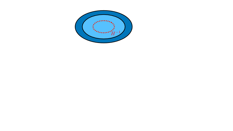
In practice, any measurement device has a finite spatial resolution that we denote . This means that experiments probing the fields and are only sensitive to their value locally averaged over a patch of size , see also Fig. 3. This leads us to introduce the coarse-grained fields
| (2.8) |
One notes that a (time-dependent) scale factor has been introduced in this expression, in order to make our formalism directly applicable to the cosmological setting in Sec. 4. In cosmology indeed, it is convenient to work with the so-called “comoving” spatial coordinate , related to the “physical” coordinate . In the above expression, and are therefore comoving while denotes a physical distance. If one is not interested in cosmological applications, one can simply set in Eq. (2.8) and in all following formulas, since the formalism presented in this section is generic (and will be specified to the cosmological setting in Sec. 4 only). In Eq. (2.8), is a window function that depends only on the distance away from in order to preserve isotropy, and which satisfies if and if . It is normalised such that
| (2.9) |
i.e. such that after coarse graining, a uniform field remains a uniform field of the same value.
Upon Fourier transforming Eq. (2.8), one obtains
| (2.10) |
which defines , that shares similar properties with . Indeed, when , the values of such that is not close to zero are much smaller than one, so one can replace in the integral over , and using the normalisation condition (2.9), one obtains in that limit. In the opposite limit where , since until , the integral over in Eq. (2.10) is at most of order , hence .
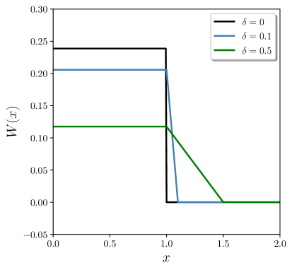
The details of between these two limits depend on those of . For instance, if is a Heaviside step function (see the black line in the left panel of Fig. 1),
| (2.11) |
where if and otherwise, and where the pre-factor is set in such a way that the normalisation condition (2.9) is satisfied, Eq. (2.10) gives rise to
| (2.12) |
This verifies the two limits given in the main text and is represented by the black line in the right panel of Fig. 1. However, the sharpness of the Heaviside profile (2.11) in real space (namely the fact that is not a continuous function) leads to mild UV divergences in some of the intermediate quantities we compute below. This suggests to use a smoother window function such as
| (2.13) |
where
| (2.14) |
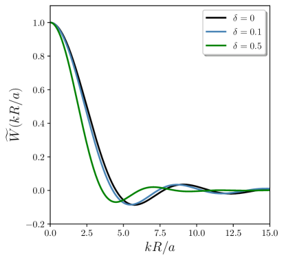
is set such that the normalisation condition (2.9) is satisfied. This generalises Eq. (2.11), which is recovered when , by adding a linear tail between and in order to make continuous. This window function is represented in the left panel of Fig. 1. From Eq. (2.10), one finds
| (2.15) |
which is represented in the right panel of Fig. 1 for different values of . One can check that this formula for the window function in Fourier space reduces to Eq. (2.12) in the limit . One can also see that, in the limit , both Eqs. (2.12) and (2.2) are such that . However, in the regime , Eq. (2.12) leads to while Eq. (2.2) leads to , which ensures UV convergence for all the quantities of interest below.
Let us also note that other smooth functions could have been employed for , for instance a Gaussian profile as often done, but as we are now going to see, the window function needs to have a compact support in order for a bipartite system to be defined with canonical commutation relations, and this makes the above choice natural. Other smooth, yet compact, window functions could obviously be considered (and tailored to better model a given experiment’s measuring device), but this would only lead to small and irrelevant modifications of the results presented in the following.
The next step consists in checking that the commutation relations (2.3) are still satisfied after coarse graining, that is to say, one should check that the coarse-graining procedure is a canonical transformation of the phase space. It is clear that one still has . Making use of Eqs. (2.8) and (2.2), one finds
| (2.16) |
Note that if the support of the window function is not bounded in real space, then the above integral is necessarily strictly positive and it is clear that one cannot get . As already mentioned, this is the reason why a compact window function was previously introduced, and hereafter, we make use of Eq. (2.13) for explicitness. The commutator (2.16) then vanishes if the two patches do not overlap, i.e. if the two spatial points are sufficiently distant away,
| (2.17) |
where denotes the (physical) distance between and , see also Fig. 3. In the coincident limit, , Eq. (2.16) gives rise to . Together with Eq. (2.13), this leads to
| (2.18) |
where and and satisfy Eq. (2.17), and where
| (2.19) |
The prefactor in this expression has been arranged such that, when , . Since the commutator (2.18) differs from Eq. (2.3), the fields need to be rescaled, and for this reason we introduce
| (2.20) |
with
| (2.21) |
One can check that is indeed canonically normalised, by explicitly calculating
| (2.22) |
Note that we have introduced a new parameter , which serves two purposes. First, it may be set in such a way that the entries of the vector share the same dimension (and, conveniently, are dimensionless), which simplifies some of the following calculations. Second, changing amounts to performing a phase-space dilatation, which is a special case of canonical transformations. Since some of the quantities we compute in the following are local-symplectic invariant, checking their non-dependence on will be a valuable sanity check.
Finally, it is interesting to calculate the two-point correlation function of the coarse-grained fields. Plugging Eq. (2.10) into (the coarse-grained version of) Eq. (2.7), one has
| (2.23) |
where we recall that is given in Eq. (2.2). This equation should be compared to Eq. (2.7), to which it reduces in the limit . The only difference is the presence of the squared window function, which originates from the fact that we have considered coarse-grained quantities.
2.3 Bipartite system
Our goal is now to characterise the presence of entanglement between the configurations of the fields at two different locations and . We therefore view our setup as a bipartite system, containing the values of the coarse-grained fields as those two locations, and arranged into the vector
| (2.28) |
The two first entries of the vector contain the phase-space variables of the “first” system, i.e. the one observed at location , while the two last entries contain the phase-space variables of the “second” system, i.e. the one observed at location . In some sense, the vector is an “enlarged” version of , which explains the notation with a capital letter. Its component will be denoted with a Latin letter, i.e. with .
It is clear that the vector suffers from the same issue as , namely that it is not canonically normalised. This problem can be solved following the considerations presented in Sec. 2.2, i.e. by defining , or
| (2.29) |
where
| (2.34) |
From Eq. (2.18), the entries of satisfy the following canonical commutation relations
| (2.35) |
the matrix being defined by
| (2.40) |
where we recall that and must satisfy Eq. (2.17). We have thus parametrised our bipartite system with canonical coordinates, which was the aim of this subsection.
2.4 Covariance matrix
As argued above, the fields being Gaussian, they are entirely described by their two-point statistics. For this reason, let us introduce the covariance matrix , defined by
| (2.41) |
which also implies that . This leads to
| (2.49) |
where the entries that are not explicitly written are obtained from the symmetry of the covariance matrix, . The invariance of the system under exchanging and also leads to an additional symmetry111In the case where the sizes of the regions centred around and are different, i.e. when , this symmetry is lost, but the same method can still be employed, see Ref. [37]. of the covariance matrix (namely under the permutation matrix that swaps the first and third, and the second and fourth, entries of the vector ), such that there are only 6 independent entries in the matrix , that we label with , , , , and . For instance, the determinant of the covariance matrix is given by
| (2.50) |
3 Mutual information and quantum discord
In Sec. 2, we have seen how a Gaussian scalar field measured at two distinct spatial locations and , coarse-grained over a spatial distance , can be described by a four-dimensional Gaussian state entirely specified by the density matrix , which is related to the power spectra of the field via Eq. (2.4). Let us now characterise the correlations that exist between measurements performed at and . This is done by means of two quantities that play an important role in quantum information theory: the mutual information that measures the amount of correlations, and the quantum discord that measures the amount of quantum correlations. Our goal is to relate those two quantities to the entries of the correlation matrix, which we have computed previously.
3.1 Mutual information
Let us first consider the case where is a classical random field. We formally denote by and the possible configurations of the field at the location and respectively. We also introduce the probability to find the field at in the configuration and similarly for . The uncertainty regarding the state of the field at can be characterised by the von-Neumann entropy
| (3.1) |
Indeed, if all vanish but one (so the configuration of the field at is certain), one can check that , and that, in general, . A similar expression for can be introduced, as well as for the joint system
| (3.2) |
where denotes the joint probability to find the field at in configuration and at in configuration . A measure of the mutual information between the configurations at the two spatial locations is given by
| (3.3) |
The fact that measures the presence of spatial correlations can be seen by noting that if the two configurations are uncorrelated, then the mutual information vanishes. Indeed, if , then , where we have used that .
Let us now translate these considerations into the quantum formalism, where our goal is to construct an analogue of . The full quantum system can be described by its density matrix , and information about the field configuration at location is obtained by tracing over the degrees of freedom corresponding to , namely
| (3.4) |
and similarly for . The state represented by is still Gaussian, and its covariance matrix is simply obtained from by removing the lines and columns corresponding to , i.e. the third and fourth lines and columns, so
| (3.7) |
where we have used the fact that, as mentioned above, the state is symmetric by exchanging and , so . The von-Neumann entropy can then be written as
| (3.8) |
with similar expressions for and . The quantity is also called the entanglement entropy of the system, and this allows us to evaluate with Eq. (3.3).
For a Gaussian state, the von-Neumann entropy is given by [38]
| (3.9) |
where the function is defined for by
| (3.10) |
and are the symplectic eigenvalues of the covariance matrix, that is to say the quantities such that . In this expression, we recall that , and is the block-diagonal matrix where each block corresponds to , and where is the dimension of phase space.
In the present situation, the symplectic eigenvalues of the full covariance matrix are given by
| (3.11) |
They allow one to rewrite Eq. (2.50) as , which also follows from the definition of the symplectic spectrum and the fact that . For the reduced states, making use of Eq. (3.7), one obtains a single symplectic eigenvalue, namely
| (3.12) |
Combining the above considerations, the mutual information is given by
| (3.13) |
Let us note that in the regime where the separation between and is large, the cardinal sine suppression in Eq. (2.4) drives , and to small values. In the limit where they can be neglected, one has , which leads to , hence more distant patches are less correlated. Another remark of interest is that the von-Neumann entropy of a pure state is known to vanish,222This is because the density matrix of a pure state is idempotent, i.e. . Using the binomial expansion, this leads to , hence (where is a positive integer). Since is defined as a Taylor series by , one has , so pure states have indeed vanishing entropy. so the mutual information between two subsystems of a pure state simply corresponds to twice the entanglement entropy.
From Eqs. (3.9) and (3.10), one can see that a state with vanishing von-Neumann entropy is one for which the symplectic eigenvalues all equal one. Here, and as will be made more explicit in Sec. 4, are not equal to one in general, denoting the fact that we are not dealing with a pure state. This may seem surprising, since in this work we consider a single scalar field , isolated from any environmental degrees of freedom, and which can therefore be placed in a pure state. The reason is the following. If the field is placed on a homogeneous background, its quantum state is separable in Fourier space, which means that there are no correlations between the Fourier subspaces and if . This was shown explicitly around Eq. (2.6). The reduced state within each Fourier subspace may therefore be pure, and within each Fourier subspace, one can study the presence of (quantum) correlations between the sectors and as subsectors of a pure state [21]. In real space however, the field generally features non-trivial correlations, see Eq. (2.7). Therefore, when restricting one’s attention to its (coarse-grained) configurations at locations and , one implicitly traces over its configuration at all other locations (to which the configurations at and are entangled), which leads to a non-pure bipartite system. In general, this effective “self-decoherence” can be measured with the purity parameter [39, 40, 41, 42]
| (3.14) |
The last expression may be used to characterise either the full system or the reduced systems , by considering the relevant symplectic eigenvalues in each case. Pure states have , while decohered states are such that . Decoherence usually leads to a suppression in the amount of quantum correlations [43]. This already hints to the fact that even if large entanglement is present in Fourier space, real-space measurements may feature less quantum correlations than those encountered in Fourier space.
3.2 Quantum discord
One way to measure the “quantumness” of the correlations between the field configurations at locations and is via quantum discord, which we now introduce. This is first done at the level of classical random variables, in the same language as the one employed at the beginning of Sec. 3.1. Upon denoting the conditional probability to find the field in configuration at location knowing that it is in configuration at , Baye’s theorem leads to . When plugging this relation into the definition (3.3) of mutual information, one obtains where we have used that . This suggests introducing the quantity
| (3.15) |
which stands for the conditional entropy contained in the field configuration at after finding the field in configuration at , averaged over all possible configurations at . The above calculation thus gives rise to an alternative expression for mutual information, namely
| (3.16) |
These considerations show that, in classical systems, .
This is however not necessarily the case in quantum systems, and the fact that vanishes for classical systems only can be used to define a criterion for the presence of quantum correlations. First, one needs to translate the conditional entropy (3.15) into the quantum formalism.
To this end, let us introduce , a complete set of projectors on the field configurations at , and denote by the quantum states on which they project. One thus has . Let us note that such complete sets of projectors (or equivalently, of states ) are not unique (for a spin particle for instance, one can consider and along any unit vector ), and this fact will be dealt with below. The probability to find the field at in the state is given by , and a measurement of the field at that returns the result projects the state into . This leads us to introducing
| (3.17) |
which is the state of the field at after measuring its configuration at and finding as a result of the measurement. The conditional entropy can thus be written as
| (3.18) |
This is the analogue of Eq. (3.15), and these formulas then allow one to evaluate with Eq. (3.16). Quantum discord is finally defined as
| (3.19) |
where minimisation is performed over all possible complete sets of projectors, in order to ensure that a non-vanishing discord signals the presence of genuine quantum correlations for any projection basis.
A generic calculation of quantum discord for Gaussian states is presented in Ref. [44]. In this article we only state the result in terms of the covariance matrix , but a detailed derivation of the formulas below can be found in this reference. Let us first denote by the off-diagonal block of the covariance matrix,
| (3.22) |
such that the covariance matrix can be written in the block form as Similarly to Eq. (3.12), we introduce
| (3.23) |
where one should note that may be positive or negative. One can show that , , and are all local-symplectic invariants, which means that they are invariant under canonical transformations that act on each sector and separately (i.e. transformations represented by block-diagonal symplectic matrices). Quantum discord, which is also a local-symplectic invariant, can therefore be written in terms of these quantities only, and after extremisation over the set of projectors appearing in Eq. (3.19) one has [44]
| (3.24) |
with
| (3.25) |
where the first equality applies if and the second one otherwise. As for the mutual information , one can check that in the limit where the configurations of the field at and are uncorrelated, , and can be neglected, hence can be neglected and one obtains [where one also has to use that , which directly follow from Eqs. (3.11) and (3.12)].
The above considerations provide all necessary formulas to explicitly compute the mutual information and the quantum discord between the field configurations at and from the knowledge of the power spectra.
4 Application to cosmological perturbations
We now consider the main question investigated in this article and use the formalism presented above to study cosmological perturbations. This will lead us to establishing important results for the detectability of quantum correlations in cosmological measurements, shedding light on our ability to prove or disprove their quantum-mechanical origin.
Let us therefore consider the case of a homogeneous and isotropic cosmology, described by the flat Friedmann-Lemaître-Robertson-Walker metric
| (4.1) |
where is the scale factor. Density fluctuations are described by the curvature perturbation [3, 45], which is a diffeomorphism-invariant combination of scalar fluctuations of the metric components and of the matter sector. On large scales, it is directly proportional to the temperature anisotropies measured on the CMB [46]. It can also be described by the Mukhanov-Sasaki variable , where where is the speed of sound ( for a scalar field) and is the first Hubble-flow parameter [47, 48], with the Hubble parameter and a dot denotes derivation with respect to cosmic time . In Fourier space, the conjugate momentum to is , where a prime denotes derivation with respect to the conformal time defined via . Each mode behaves as a parametric oscillator, with equation of motion
| (4.2) |
The standard cosmological scenario starts with a phase of accelerated expansion () called cosmic inflation, during which quantum vacuum fluctuations are gravitationally amplified and stretched to astrophysical distances, which seeds the cosmological structures we later observe. In what follows, we study the quantum correlations contained in cosmological perturbations during this early epoch of inflation, and during the subsequent era where the universe is dominated by radiation.
4.1 Inflationary era
4.1.1 Calculation of the covariance matrix
During inflation, measurements of the CMB constrain the expansion of the universe to proceed close to the de-Sitter regime where . The Mukhanov-Sasaki equation (4.2) thus reads , the solution of which is given by
| (4.3) |
Here, the mode function has been normalised to the Bunch-Davies vacuum [49], i.e. the integration constants are set such that in the asymptotic past, matches the Minkowski vacuum. The momentum conjugated to is
| (4.4) |
Hereafter we make the identification and , but one should recall that since the quantities introduced in Sec. 3 are local-symplectic invariants, the following calculations do not depend on the choice of canonical variables. In other words, one may perform any canonical transformation (for instance, describe the system with the curvature fluctuation and its conjugate momentum) without affecting the result. The reason why we choose to work with the Mukhanov-Sasaki variable is one of convenience, and Eqs. (4.3) and (4.4) lead to the reduced power spectra
| (4.5) |
One can check that , which confirms the remark made at the end of Sec. 3.1 that each Fourier mode is placed in a pure state. Indeed, recalling Eq. (2.41), it implies that the determinant of the covariance matrix describing a given Fourier mode is one, so the purity equals one too, see Eq. (3.14).
When computing the covariance matrix via Eq. (2.4), one may note that some of the integrals over are IR-divergent, i.e. they diverge when . Indeed, as noticed below Eq. (2.2), when , , and one also has as soon as . From Eq. (4.5), one thus finds that and are logarithmically divergent. The reason why this divergence does not appear in practice is the following. Any local observer only has access to a finite region of the universe, and we let denote the size of the observable universe. In terms of more usual cosmological parameters, it can be written as
| (4.6) |
where is the number of -folds spent outside the Hubble radius by the largest observable scales (it is typically of order at the end of inflation), and denotes the almost-constant value of the Hubble parameter during inflation. In practice, “fluctuations” are perceived as deviations of the fields from the mean value measured inside the observable patch, i.e. one only has access to
| (4.7) |
where represents the location of the observer. Making use of Eq. (2.10), this gives rise to
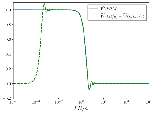
| (4.8) |
This means that, once the finite size of the observable universe is taken into account, the window function becomes . Because of the generic properties of the function discussed below Eq. (2.10), when , i.e. for wavenumbers inside the observable patch, this does not modify the window function substantially. However, when , the two terms in the effective window function cancel out each other, which implies that unobservable modes, i.e. those above the observed region, are filtered out. This is confirmed by Fig. 2 where both and are displayed as a function of . The effective window function thus selects out modes such that .
Hereafter, the finite size of the observable universe is taken into account by simply adding a lower bound to all -integrals at , i.e. the effective window function one considers is . The reason is that the details of the terms coming from this lower bound only play a minor role in the formulas derived below, especially when considering the relevant limit . In practice, this solves the IR divergence mentioned above.
With Eq. (4.5) for the power spectra, the entries of the covariance matrix given in Eq. (2.4) read
| (4.9) | ||||
| (4.10) | ||||
| (4.11) | ||||
| (4.12) |
In these expressions, we have introduced a few relevant parameters and useful notations that we now describe (see also Fig. 3). The parameter denotes the distance between the two patches in units of ,
| (4.13) |
where the lower bound comes from Eq. (2.17). The parameter corresponds to the lower bound imposed on in order to take into account the finite size of the observable universe, i.e.
| (4.14) |
The condition comes from the fact that one cannot coarse-grain over distances larger than those observable, but the relevant regime really is (for instance, in CMB measurements, is of the order of the inverse of the maximal multipolar moment , and is even much smaller for measurements of the large-scale structure performed at smaller redshifts). Finally, since the power spectra (4.5) only feature power-law functions of the wavenumber, the covariance matrix only involves integrals of the type
| (4.15) | ||||
| (4.16) | ||||
| (4.17) |
where the integral has also been introduced since it will be needed in the calculation of Sec. 4.2 where the covariance matrix is obtained in the radiation-dominated era. Since the window function (2.2) involves trigonometric and power-law functions of , these three integrals can be expressed solely in terms of the cosine integral function, see Appendix A for details and explicit formulas.
The above expressions (4.9), (4.10), (4.11) and (4.12) of the covariance matrix are quite involved and, as a consequence, it is interesting to derive analytical approximations for the relevant physical quantities. One can check that the factors and appearing in Eq. (4.9) cancel out when computing the symplectic values,333The fact that cancels out is expected from the above remark that it simply corresponds to a local canonical redefinition of the phase-space variables, and the independence on follows from the fact that it can be re-absorbed by a rescaling of . so their values depend only on four parameters, namely , , and . As explained around Eq. (4.13), one must have , so it is interesting to consider the limit which corresponds to the situation where the two observed patches are well separated, i.e. . The parameter , defined in Eq. (4.14), corresponds to the ratio between the size of the observed patches and the size of the entire observable universe, which is why, as already mentioned, the regime is of interest. Finally, is a parameter that describes the edge of the window function in real space. It is smaller than one for experiments with a sharp filtering device, so for convenience we expand our results in too, although the precise value of is of little importance in what follows, as long as it remains of order one or smaller. Let us note that , so when the observed patches are well within the observable universe. This is why one should first expand in , and then in before finally expanding in . When doing so, in Appendix A, approximate expressions for the integrals and are obtained. Plugging the result into Eq. (4.9), (4.10), (4.11) and (4.12), one obtains
| (4.18) | ||||
| (4.19) | ||||
| (4.20) | ||||
| (4.21) | ||||
| (4.22) | ||||
| (4.23) |
where we have set for convenience, see footnote 3. On top of the parameters already mentioned, these expressions also involve the combination , and different regimes for the value of that parameter will have to be distinguished below.
4.1.2 De Sitter mutual information
Having established the relevant expressions for the covariance matrix, one can now determine the symplectic values , , and , and the mutual information. Since we are far from resolving the Hubble radius during inflation (that would imply to measure the CMB up to multipoles ), the relevant limit is . Plugging Eqs. (4.18)-(4.23) into Eqs. (3.11), (3.12) and (3.23), one obtains
| (4.24) | ||||
| (4.25) | ||||
| (4.26) | ||||
| (4.27) |
One can check that , and are all positive under the conditions where this limit has been taken, which is a good consistency check (recall that the sign of is not constrained).
Let us now compute the mutual information . One can see that , and are all large and of the same order . This means that the function appearing in Eq. (3.13), and defined in Eq. (3.10), needs to be evaluated with large arguments. Using that when , Eq. (3.13) gives rise to , which leads to
| (4.28) |
One can see that the dependence on the parameters of the problem is very mild, and that the result does not depend on at that order. In the limit where the logarithmic terms dominate over the constant terms, a rough version of the above formula is given by
| (4.29) |
which makes this mild dependence even more explicit (parameters only appear through logarithms of logarithms), and in which no longer appears. These approximated formulas are compared with a full numerical calculation of the mutual information in Fig. 4. One can see that, in the regime , the approximations indeed provide an excellent fit to the exact result. Even if Eq. (4.1.2) is more accurate than Eq. (4.29) as expected, Eq. (4.29) still provides a correct estimate sufficiently far away from the boundaries of the interval in which is allowed to vary.
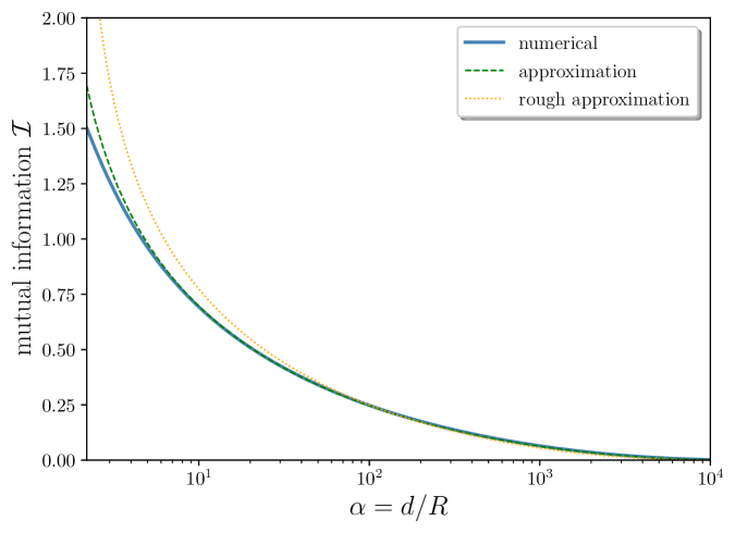
One concludes that the mutual information between two patches of the universe during inflation is of order one, at least in the regimes of observational relevance. As already mentioned, its dependence on the distance is very mild, especially when compared to the flat spacetime case, where it is known to decay at its inverse fourth power, see Ref. [37]. This is because, in the case of inflation (de Sitter spacetime), quantum correlations are now produced in Fourier space, as revealed by the fact that the quantum state of the perturbations is no longer a two-mode coherent state but a two-mode squeezed state, which is an entangled state. We will come back to this comparison when we compute the quantum discord later on in this section.
Let us also recall that the mutual information between curvature perturbations with opposite Fourier modes, and , was computed in Ref. [21] and was found to be of order
| (4.30) |
where is the wavelength associated to the mode , assuming that it is much larger than the Hubble radius (so . For the wavenumbers observed in the CMB, is of order at the end of inflation, so , which is much larger than the typical values encountered in Fig. 4. The reason is that, while depends logarithmically on the relevant scales of the problem, involves the logarithm of the logarithm of those scales, see Eq. (4.29). This shows that the amount of correlations being accessed is smaller in real space than in Fourier space.
As explained around Eq. (3.14), another difference between correlations in real and Fourier spaces is that, while the curvature perturbations with opposite wavevectors are placed in a pure state, and decouple from any other set of opposite wavevectors, in real space, the system is in a mixed state, since one has implicitly traced over the value of the field at any other spatial location, to which the system nonetheless couples. This effective “self-decoherence” can be assessed with the purity parameter defined in Eq. (3.14), and the fact that the symplectic eigenvalues are large in this regime means that the purity parameter is small, hence that the system we consider here is strongly mixed. More precisely, the purity associated with the two-point setup is given by while the purity for the one-point systems is given by .
Finally, although the regime cannot be probed in the CMB as argued above, it is still of theoretical interest to discuss this limit, in order to fully describe the structure of the correlations present in the field of inflationary perturbations. In this regime, Eqs. (4.18)-(4.23) lead to . Since these three symplectic values are the same, the mutual information vanishes at leading order, see Eq. (3.13). At next-to-leading order, when , one finds , and when , one has , which coincides with the result obtained in the Minkowski vacuum, see Refs. [19, 37]. For comparison, the mutual information between curvature perturbations with opposite Fourier modes is given by in this regime , see Ref. [21], so one finds that it is suppressed too. Let us note that the fact that the symplectic eigenvalues are of order one also means that the system we consider is almost pure. From Eq. (3.14), one indeed obtains and with . This is in contrast with the opposite regime where we had found that the system is in a strongly mixed state.
4.1.3 De Sitter quantum discord
Let us now compute the quantum discord. Having already determined , this means that we need to calculate . In the regime , Eqs. (4.24), (4.25), (4.26) and (4.27) imply that , and are all of order , while is of order and is therefore suppressed compared to , and . This means that, in the quantity appearing below Eq. (3.25) whose sign determines which formula one should use for , and which is written as the difference of two positive terms, the first term is of order and the second term is of order . Which term dominates thus depends on how compares to , and this implies that the cases and need to be distinguished.
Let us first consider the case where . In this case, the discriminating quantity appearing in the text after Eq. (3.25) is negative, hence the second formula for needs to be used. This leads to at leading order, so is of order and is therefore large. Using that when , this gives rise to , which coincides with the expression obtained for . This means that, at leading order, there is an exact cancellation between and . Since both and are of order one, this implies that the quantum discord, which must come from higher-order terms, is a suppressed quantity in this regime.
In order to compute its value, one needs to work at next-to-leading order, where . For the mutual information , Eq. (3.13) yields
| (4.31) |
while for , Eq. (3.24) leads to , which gives rise to
| (4.32) |
In this expression, the second term is of order while the third term is of order . Since we work under the assumption , the third term can therefore be neglected, and the quantum discord (3.19) is given by
| (4.33) |
This shows that the discord is of order in this regime. An explicit expression can be obtained upon using Eq. (4.24), but since it is rather cumbersome, let us give only its “rough” version where the logarithms are assumed to dominate over terms of order one [i.e. similarly to what was done in Eq. (4.29)],
| (4.34) |
We now turn to the case . In this case, the discriminating quantity appearing below Eq. (3.25) is positive, hence the first formula for needs to be used. At leading order, it still gives rise to , so the cancellation between and is still encountered in that case, and the discord is again suppressed. At next-to-leading order, Eq. (4.31) can still be used, while Eq. (3.25) leads to
| (4.35) |
In this expression, the second term is of order while the third term is of order one. Since we work under the assumption that , the third term can be discarded, which leads to
| (4.36) |
The correction to is thus of order , while the correction to is of order , see Eq. (4.31). In the regime , the correction to thus provides the dominant contribution, and one obtains
| (4.37) |
The discord is therefore suppressed by in this regime. More precisely, an explicit expression can be obtained upon using Eq. (4.24), and in the “rough” limit where the logarithmic terms dominate over terms of order one, one finds
| (4.38) |
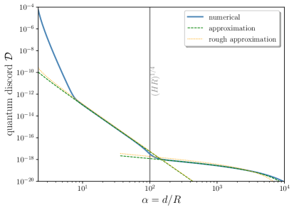
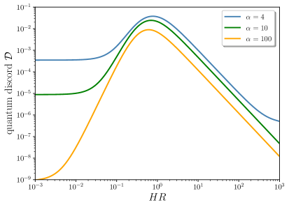
The above formulas are displayed in the left panel of Fig. 5 where they are compared with a numerical calculation. They are also summarised in Fig. 7 below. One can check that, as for the mutual information , they provide a good fit to the full result, even when approaches its upper bound . When is close to its lower bound (4.13), the approximation we have developed (which assumes under-estimates the discord, which is also where the discord reaches its maximal value. For this reason, in the right panel of Fig. 5, we have displayed the discord for a few values of not too far from its lower bound. At large values of , one recovers the behaviour derived around Eq. (4.34), and at small values of , the quantum discord is, like the mutual information , of order (see the discussion at the beginning of this section). In between, one can see that it reaches a maximum value when is of order one. This configuration of maximal discord, where both and are of order one, cannot be described by our approximations and one needs to resort to a numerical calculation.
4.1.4 Discussion
At this point, it is worth drawing lessons from the results obtained before. The first conclusion that we reach is that the discord produced in real space during inflation is non-vanishing and that, therefore, “discord transfer” does indeed take place from Fourier to real space.
The second conclusion concerns the amplitude of the discord in real space. Clearly, for reasons already presented, it is small; in any case, smaller than the discord between opposite Fourier modes, which is half of the mutual information given in Eq. (4.30), see Ref. [21], and is therefore large for super-Hubble scales.
Finally, the real-space mutual information and quantum discord in de Sitter spacetime found above should also be compared to the corresponding result in flat (Minkowski) spacetime, see Ref. [37]. Indeed, to some extent, the Minkowski result represents the benchmark to which other calculations should be set against.
In Minkowski Fourier space, no mutual information and no discord is produced because, in flat spacetime, the field always remains in its vacuum state. As a consequence, in this case, the mutual information and discord in real space (if present) only originate from the fact that we have traced out field values at other spatial location. In this sense, the amount of correlations calculated in Minkowski, see Ref. [37], represents the minimum that is always present in a system due to the passage from Fourier to real space. The “genuine” correlations, originating from a physical phenomenon that can produce entangled quanta in Fourier space (such as interaction with an exterior classical source, as during inflation), must therefore appear as an “additional” contribution.
Let us first note that both in Minkowski space and in de-Sitter space, when , the mutual information acquires a finite value (that however depends on the background one considers) while quantum discord vanishes. The reason for this similarity can be understood as follows. When takes a non-vanishing value, the window function in Fourier space decays more rapidly, namely if , see Eq. (2.12), while if , see Eq. (2.2). The case thus corresponds to larger UV contributions, and since the de-Sitter and Minkowski space-times are identical at small scales, this explains the similar behaviours.
There are however differences. In Ref. [37], it was established that, in the Minkowski space-time, both the mutual information and the quantum discord are of order at large distances (unless , in which case the discord vanishes as mentioned above). In de Sitter, in that limit, we have shown that mutual information remains of order if and of order one if , and that quantum discord remains of order if and of order if . Both are therefore larger in de Sitter than in Minkowski. Therefore, a third conclusion is that, despite the fact that the de Sitter mutual information and discord are smaller in real space than in Fourier space, they are nevertheless always larger than their flat space-time counterpart. This somehow expected result confirms that non-trivial quantum correlations are produced during inflation.
4.2 Radiation era
Let us now study how the correlations contained in the field of cosmological perturbations evolve after inflation, when the universe is dominated by a radiation fluid. During that epoch, the scale factor evolves linearly with conformal time, i.e. . Upon requiring that the scale factor and its derivative are continuous at the transition between inflation and the radiation epoch, the two integration constants and can be determined, and one obtains and , where and are the values of and at the end of inflation. Regarding cosmological perturbations, the Mukhanov-Sasaki equation (4.2) should now be solved with and , and the generic solution reads
| (4.39) |
where and are two integration constants that must be set by requiring continuity of the first and second fundamental forms [50]. Those matching conditions take a complicated form in general, but let us recall that the filtering procedure is such that scales below the coarse-graining radius, i.e. such that , are filtered out. Given that, as argued below Eq. (4.18), we are very far from resolving the Hubble radius at the end of inflation, , all relevant scales are such that , i.e. they are larger than the Hubble radius at the end of inflation. One can therefore restrict the analysis of the matching conditions to this regime, where they simply boil down to requiring the continuity of the curvature perturbation and of the Bardeen potential [51]. At leading order in , this leads to
| (4.40) |
where is the value of the first Hubble-flow parameter during inflation. The conjugated momentum is given by
| (4.41) |
4.2.1 Covariance matrix
Making use of Eq. (2.6), the reduced power spectra can then be computed. Upon introducing , they are given by
| (4.42) | ||||
| (4.43) | ||||
| (4.44) |
One may note that these expressions yield while, as argued below Eq. (4.5), this combination of the power spectra should equal . This is because the matching conditions have been performed at leading order in only, while the result comes from higher-order terms. Since they play a negligible role hereafter, they can be safely neglected.
The reduced power spectra involve power-law and trigonometric functions of the wavenumber. As a consequence, the entries of the covariance matrix can still be expressed in terms of the three integrals , and introduced in Eq. (4.15) and further studied in Appendix A. One obtains
| (4.45) | ||||
| (4.46) | ||||
| (4.47) | ||||
| (4.48) | ||||
| (4.49) | ||||
| (4.50) |
where we have defined for notational convenience. Let us note that contrary to inflation where is almost constant, decreases with time in the radiation era (one has ), so is a time-dependent parameter.
4.2.2 Analytical approximations
The above formulas allow one to compute all relevant quantities introduced in Sec. 3. However, as during inflation, analytical approximations are useful to gain insight in the result. The considerations presented in Sec. 4.1 about , and still apply here, so the regime of interest is the one where . Regarding , the situation is more subtle. Although, as argued above, , decreases during the radiation era, hence decreases too. At the time of recombination where the CMB is emitted, is large below the first recombination peak, so for multipoles , and small above. The two regimes and need therefore to be considered. Moreover, in Eqs. (4.2.1)-(4.2.1), the combinations appear in the last arguments of some of the and integrals, the approximate value of which thus depends on which of and is the largest. This adds a second pivotal value for at , so one has to consider three different regimes depending on the value of .
Below, we review these three regimes one after the other, making use of the approximated formulas derived in Appendix A for the integrals , and , and employing similar techniques as in Sec. 4.1. Let us note that the approximations of Appendix A are valid when the absolute value of the last argument of the integrals , and is much smaller than (since the expansion in is performed first). As argued in Sec. 4.1, this is the case when the last argument is of order , and if , this is also true since given that observations encompass many Hubble patches at the time of recombination.
Case .
This regime corresponds to and , so both the size of the patch and the distance between the two patches lie inside the Hubble radius. Plugging the approximations of Appendix A into Eqs. (4.45)-(4.2.1), one obtains
| (4.51) | ||||
| (4.52) | ||||
| (4.53) | ||||
| (4.54) | ||||
| (4.55) | ||||
| (4.56) |
where the expansion of , , and has been performed at next-to-leading order to deal with the cancellation at leading order when evaluating and in the expression (3.11) for . These formulas give rise to the symplectic values
| (4.57) | ||||
| (4.58) | ||||
| (4.59) | ||||
| (4.60) |
In order to estimate the size of these parameters, let us introduce the length scale that corresponds to the Hubble radius at the end of inflation, so and . As argued below Eq. (4.18), we are far from resolving such scales, so
| (4.61) |
During the radiation epoch, and this allows one to write . In this expression, , and , therefore . The other symplectic values are such that . Since we have assume , those parameters are much larger than , hence much larger than one too.
In this regime of large symplectic values, as explained in Sec. 4.1, the one-point and two-point systems are placed in strongly mixed states. The mutual information can be computed from Eq. (4.31), which here gives rise to
| (4.62) |
where we use the same “rough” approximation as in Sec. 4.1. A crucial difference with Eq. (4.29) obtained during inflation is that, here, the mutual information depends logarithmically on , and not only on logarithms of logarithms. This means that, contrary to what happens during inflation, a substantial amount of mutual information can be accessed during the radiation era.
For the quantum discord, in the regime , we are in the first condition of Eq. (3.24), which leads to at leading order, hence and cancel out and the discord vanishes at leading order like during inflation. At next-to-leading order, Eq. (3.24) yields the same expression as in Eq. (4.35) for ; and although the hierarchy between the symplectic values is different here, it turns out that the dominant term is still the same and we have , which gives rise to . Then, making use of Eq. (4.31), one obtains the same formula as in Eq. (4.37). In the present context, this formula leads to
| (4.63) |
One notices that is of the same order as , and is therefore tiny since we have argued above that , see the discussion around Eq. (4.61).
Case
This regime corresponds to but , so the size of the patches is sub-Hubble but the distance between the two patches is super-Hubble. In this regime, the same expressions for , and as those given in Eqs. (4.51)-(4.56) are found, and the remaining entries of the covariance matrix are given by
| (4.64) | ||||
| (4.65) | ||||
| (4.66) |
For the symplectic values, the same expression for as the one given in Eq. (4.57) is obtained, and the remaining , and parameters read
| (4.67) | ||||
| (4.68) | ||||
| (4.69) |
One thus finds that , and are all of order and are therefore large, as argued below Eq. (4.61). Regarding , it is much smaller than the other three parameters since one has . One must therefore expand the mutual information and the quantum discord in the regime and . The one-point and the two-point systems are still in a strongly mixed state, and making use of Eq. (4.31) for the mutual information, one finds at leading order
| (4.70) |
As during inflation, the mutual information is given by a logarithm of a logarithm, and is therefore of order one.
Regarding quantum discord, under the condition (4.61), one can show that the discriminating quantity appearing below Eq. (3.25) is positive, and that , which gives rise to . The same expression of in terms of the symplectic values is obtained as the one given in Eq. (4.63), which here reduces to
| (4.71) |
One thus finds that the discord is of order in this regime. Since both and are large, this means that the discord is again tiny.
Case
In this case, both the size of the patches and the distance between them is larger than the Hubble radius. Plugging the approximations of Appendix A into Eqs. (4.45)-(4.2.1), one obtains
| (4.72) | ||||
| (4.73) | ||||
| (4.74) |
while , and are still given by Eq. (4.64). From these expressions, the symplectic values can be approximated by
| (4.75) | ||||
| (4.76) | ||||
| (4.77) |
where is still given by Eq. (4.69). We are therefore in the regime where . The situation is thus the same as in the previous case, namely the case . The mutual information is thus given by Eq. (4.31), which here leads to
| (4.78) |
at leading order, and the quantum discord can be obtained from Eq. (4.63), which reduces to
| (4.79) |
One thus finds that the mutual information is of order one, while quantum discord is strongly suppressed in this regime.
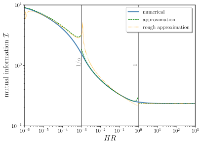
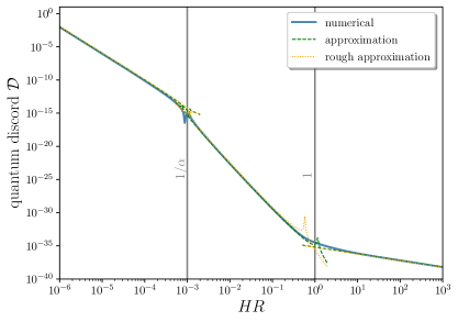
The above analytical approximations are compared with a numerical evaluation of the full formulas in Fig. 6. One can check that they provide indeed a good description of the full result. This confirms that, at the scales observed in the CMB, the mutual information and/or the quantum discord in real space are non-vanishing but suppressed compared to their typical values in Fourier space. The formulas derived in this section are also summarised in Fig. 7 where order-one and logarithmic prefactors have been removed for clarity.
5 Conclusion
In this work, we have calculated, in real space, the mutual information and the quantum discord of cosmological curvature perturbations, during an early phase of cosmic inflation and during the subsequent radiation era. Our goal was to give a first estimate of the amount of quantum correlations present in the CMB, in real space. In order to carry out this task, we have used the framework outlined in Ref. [37], which provides a mean to calculate, in real space, the mutual information and the quantum discord contained in free quantum fields. We derived explicit and exact analytical expressions, for which we then obtained analytical approximations, confirmed by numerical computations.
Our main results are summarised in Fig. 7. During inflation, when the distance between the two measured patches of size is smaller than the Hubble radius , both and are non-vanishing but suppressed by . This coincides with the result obtained in the Minkowski vacuum, see Ref. [19] and Ref. [37]. When is larger than the Hubble radius but is not, both and are suppressed by . Otherwise, when both the size of the patches and the distance between them is larger than the Hubble radius, the mutual information is of order one while quantum discord is suppressed by inverse powers of and . During the radiation epoch, the mutual information can be substantial when , and is of order one otherwise. However, the quantum discord is always highly suppressed, at least when is larger than the redshifted size of the Hubble radius at the end of inflation (recall that we are far from probing such scales). Note that in the specific case where the window function is sharp in real space (), both in Minkowski and in de Sitter, we found that the quantum discord vanishes.
Our main conclusion is therefore that, with measurements of the CMB, for reasonable (current and future) spatial resolution, even though a non-vanishing amount of entanglement entropy or quantum discord in real space exists, these quantities are highly suppressed.
This statement may seem at odd with the fact that in Fourier space, free quantum fields evolving on curved backgrounds undergo creation of pairs of entangled particles with wavevectors and , such that for the bipartite system , a very substantial amount of mutual information and quantum discord is reached on super-Hubble scales [21]. A crucial difference between the and the systems is however that, since different Fourier modes decouple for a free field evolving on a homogeneous background, the systems are placed in a pure state, and the quantum state of the full field is a direct product of pure states, one for each set . In real space however, correlations build up between the field configuration at different spatial locations. As a consequence, by considering the system , one implicitly traces over the configuration of the field at any location different from and , which implies that the bipartite system is placed in a mixed state. This effective “self-decoherence” leads to a suppression of quantum discord (at the technical level, we have seen that large symplectic eigenvalues are indeed both associated with a small purity parameter and to an exact cancellation between and at leading order).
The situation depicted in Fig. 7 could therefore be summarised as follows. For scales remaining inside the Hubble radius throughout the entire cosmic evolution, there is no creation of pairs of entangled particles, hence, although the real-space bipartite system is in a quasi pure state, the mutual information and the quantum discord remain small. For scales stretched above the Hubble radius, a large amount of entangled particles are created in each Fourier mode, but “self-decoherence” leads to an important suppression of the quantum discord.
There is, however, one exception to this general conclusion, namely those scales that cross the Hubble radius at the end of inflation, and that undergo particle creation only for a brief period around that time. The real-space bipartite systems at those scales are in a quasi pure state, and if is not much larger than (namely the two measured patches are close one to another, in units of their size), both the mutual information and the quantum discord is of order one or slightly below, see the right panel of Fig. 5. Such scales are too small to be accessed in CMB measurements, as well as in measurements of the large-scale structures performed at smaller redshift. The only possibility would be that primordial black holes [52] form straight after the end of inflation from the amplification of those scales, as may occur e.g. as a result of the preheating instability [53, 54, 55, 56].
The conclusions reached in the present article should also be compared to what is obtained in Minkowski (flat) spacetime. In this case, there is no quantum discord at all in Fourier space since the fields always remain in their vacuum state. In real space, the discord also vanishes for sharp window functions but can be non-zero for smoother window functions, in which case it scales as the inverse of the fourth power of the distance between the two patches [37]. Summarising, the mutual information and quantum discord found in cosmology are, unsurprisingly, always larger than in flat spacetime.
It may also be noticed that estimating or gauging how much of mutual information and/or of quantum discord is needed to be able to measure quantum correlations in a system is not obvious (even if, of course, the larger the discord, the higher the chance to observe a signature) since it may depend on the system, the experimental protocol, the precision of the detector and so on. Therefore, a priori, a small amount of quantum discord does not necessarily rule out the possibility to highlight the quantum origin of the perturbations in real space. On the other hand, the fact that the discord is not vanishing does not guarantee, even in principle, that quantum effects can be detected. For instance, it remains to be seen if the Bell’s inequality can be violated in real space, since a non-vanishing discord for mixed states does not necessarily imply quantum entanglement [57].
To close this article, let us acknowledge that the results obtained here certainly indicate that revealing the quantum origin of the cosmological perturbations is not an easy task, especially at CMB scales. We have argued that it might be more feasible on much smaller scales. However, even if ultra-light black holes were detected (possibly through the emission of an associated gravitational-waves background [58]), it would remain to determine which measurable quantities could unveil the quantum nature of the underlying overdensity field, and we leave this discussion to future work.
Appendix A Approximation for the trigonometric integrals
In this appendix, we explain how to calculate and approximate the three integrals (4.15), (4.16) and (4.17) defining the functions , and . Since the window function (2.2) involves trigonometric and power-law functions of , these three integrals can be expressed solely in terms of
| (A.1) | ||||
| (A.2) |
Explicitly, after long but straightforward calculations, one indeed arrives at the following expressions
| (A.3) | ||||
| (A.4) | ||||
| (A.5) |
The functions and can be performed in terms of the cosine integral function,
| (A.6) |
when is a positive integer number. In practice, the values of that are relevant for the calculation presented in the main text are for , and for . For those values, one has
| (A.7) | ||||
| (A.8) | ||||
| (A.9) | ||||
| (A.10) | ||||
| (A.11) | ||||
| (A.12) | ||||
| (A.13) | ||||
| (A.14) | ||||
| (A.15) | ||||
| (A.16) |
These expressions are useful to evaluate the integrals , and numerically. In the regime where , they can be expanded, making use of the Taylor expansion of the cosine integral function
| (A.17) |
where is the Euler constant. This gives rise to
| (A.18) | ||||
| (A.19) | ||||
| (A.20) | ||||
| (A.21) | ||||
| (A.22) | ||||
| (A.23) | ||||
| (A.24) | ||||
| (A.25) | ||||
| (A.26) | ||||
| (A.27) |
The reason why the integrals have been expanded to such a high order in is that all negative powers of cancel out in the integrals , and when , which only feature mild (i.e. logarithmic) divergence in . Plugging the above formulas into Eq. (A), one indeed obtains
| (A.28) | ||||
| (A.29) | ||||
| (A.30) | ||||
| (A.31) |
where the result is also expanded in (explicit expressions where is left free can be obtained but they are rather cumbersome). For the integrals and , one further expands in (after expanding in ), so two regimes need to be distinguished.
The first regime is when . In this case, the integrals of interest are
| (A.32) | ||||
| (A.33) | ||||
| (A.34) | ||||
| (A.35) |
The fact that we have first expanded in and then in means that those expressions only apply when , and one can check that this is always verified for the cases of interest in the main text, since and (namely the observable region contains many Hubble patches at the time of recombination).
The second regime of interest is defined by the condition . In this case, the integrals of interest are
| (A.36) | ||||
| (A.37) | ||||
| (A.38) | ||||
| (A.39) | ||||
| (A.40) | ||||
| (A.41) |
References
- [1] G. Adesso, S. Ragy and A. R. Lee, Continuous variable quantum information: Gaussian states and beyond, arXiv e-prints (Jan., 2014) arXiv:1401.4679, [1401.4679].
- [2] A. A. Starobinsky, Spectrum of relict gravitational radiation and the early state of the universe, JETP Lett. 30 (1979) 682–685.
- [3] V. F. Mukhanov and G. V. Chibisov, Quantum Fluctuations and a Nonsingular Universe, JETP Lett. 33 (1981) 532–535.
- [4] S. W. Hawking, The Development of Irregularities in a Single Bubble Inflationary Universe, Phys. Lett. B115 (1982) 295.
- [5] A. A. Starobinsky, Dynamics of Phase Transition in the New Inflationary Universe Scenario and Generation of Perturbations, Phys. Lett. B117 (1982) 175–178.
- [6] A. H. Guth and S. Y. Pi, Fluctuations in the New Inflationary Universe, Phys. Rev. Lett. 49 (1982) 1110–1113.
- [7] J. M. Bardeen, P. J. Steinhardt and M. S. Turner, Spontaneous Creation of Almost Scale - Free Density Perturbations in an Inflationary Universe, Phys. Rev. D28 (1983) 679.
- [8] A. A. Starobinsky, A New Type of Isotropic Cosmological Models Without Singularity, Phys. Lett. B91 (1980) 99–102.
- [9] K. Sato, First Order Phase Transition of a Vacuum and Expansion of the Universe, Mon. Not. Roy. Astron. Soc. 195 (1981) 467–479.
- [10] A. H. Guth, The Inflationary Universe: A Possible Solution to the Horizon and Flatness Problems, Phys. Rev. D23 (1981) 347–356.
- [11] A. D. Linde, A New Inflationary Universe Scenario: A Possible Solution of the Horizon, Flatness, Homogeneity, Isotropy and Primordial Monopole Problems, Phys. Lett. B108 (1982) 389–393.
- [12] A. Albrecht and P. J. Steinhardt, Cosmology for Grand Unified Theories with Radiatively Induced Symmetry Breaking, Phys. Rev. Lett. 48 (1982) 1220–1223.
- [13] A. D. Linde, Chaotic Inflation, Phys. Lett. B129 (1983) 177–181.
- [14] Planck collaboration, Y. Akrami et al., Planck 2018 results. X. Constraints on inflation, 1807.06211.
- [15] D. Sudarsky, Shortcomings in the Understanding of Why Cosmological Perturbations Look Classical, Int. J. Mod. Phys. D 20 (2011) 509–552, [0906.0315].
- [16] A. Bassi and G. C. Ghirardi, Dynamical reduction models, Phys. Rept. 379 (2003) 257, [quant-ph/0302164].
- [17] H. Casini and M. Huerta, Remarks on the entanglement entropy for disconnected regions, JHEP 03 (2009) 048, [0812.1773].
- [18] A. Datta, Quantum discord between relatively accelerated observers, Phys. Rev. A 80 (Nov., 2009) 052304, [0905.3301].
- [19] N. Shiba, Entanglement Entropy of Two Spheres, JHEP 07 (2012) 100, [1201.4865].
- [20] E. A. Lim, Quantum information of cosmological correlations, Phys. Rev. D91 (2015) 083522, [1410.5508].
- [21] J. Martin and V. Vennin, Quantum Discord of Cosmic Inflation: Can we Show that CMB Anisotropies are of Quantum-Mechanical Origin?, Phys. Rev. D93 (2016) 023505, [1510.04038].
- [22] S. Kanno, J. P. Shock and J. Soda, Quantum discord in de Sitter space, Phys. Rev. D 94 (2016) 125014, [1608.02853].
- [23] E. Bianchi, L. Hackl and N. Yokomizo, Linear growth of the entanglement entropy and the Kolmogorov-Sinai rate, JHEP 03 (2018) 025, [1709.00427].
- [24] L. Espinosa-Portalés and J. García-Bellido, Entanglement entropy of Primordial Black Holes after inflation, Phys. Rev. D 101 (2020) 043514, [1907.07601].
- [25] L. Espinosa-Portalés and J. García-Bellido, Long range enhanced mutual information from inflation, 2007.02828.
- [26] L. Henderson and V. Vedral, Classical, quantum and total correlations, 0105028.
- [27] H. Ollivier and W. H. Zurek, Quantum Discord: A Measure of the Quantumness of Correlations, Phys. Rev. Lett. 88 (2001) 017901.
- [28] J. Martin and V. Vennin, Bell inequalities for continuous-variable systems in generic squeezed states, Phys. Rev. A 93 (2016) 062117, [1605.02944].
- [29] J. Martin and V. Vennin, Obstructions to Bell CMB Experiments, Phys. Rev. D 96 (2017) 063501, [1706.05001].
- [30] K. Ando and V. Vennin, Bipartite temporal Bell inequalities for two-mode squeezed states, Phys. Rev. A 102 (2020) 052213, [2007.00458].
- [31] D. Campo and R. Parentani, Inflationary spectra and violations of Bell inequalities, Phys. Rev. D 74 (2006) 025001, [astro-ph/0505376].
- [32] J. Maldacena, A model with cosmological Bell inequalities, Fortsch. Phys. 64 (2016) 10–23, [1508.01082].
- [33] S. Kanno and J. Soda, Infinite violation of Bell inequalities in inflation, Phys. Rev. D 96 (2017) 083501, [1705.06199].
- [34] S. Choudhury, S. Panda and R. Singh, Bell violation in the Sky, Eur. Phys. J. C 77 (2017) 60, [1607.00237].
- [35] R. de Putter and O. Doré, In search of an observational quantum signature of the primordial perturbations in slow-roll and ultraslow-roll inflation, Phys. Rev. D 101 (2020) 043511, [1905.01394].
- [36] J. Martin and V. Vennin, Leggett-Garg Inequalities for Squeezed States, Phys. Rev. A 94 (2016) 052135, [1611.01785].
- [37] J. Martin and V. Vennin, Real-space entanglement of quantum fields, 2106.14575.
- [38] A. S. Holevo and R. F. Werner, Evaluating capacities of Bosonic Gaussian channels, arXiv e-prints (Dec., 1999) quant–ph/9912067, [quant-ph/9912067].
- [39] W. H. Zurek, Pointer basis of quantum apparatus: Into what mixture does the wave packet collapse?, Phys. Rev. D 24 (Sep, 1981) 1516–1525.
- [40] W. H. Zurek, Environment-induced superselection rules, Phys. Rev. D 26 (Oct, 1982) 1862–1880.
- [41] E. Joos and H. Zeh, The Emergence of classical properties through interaction with the environment, Z. Phys. B 59 (1985) 223–243.
- [42] T. Colas, J. Grain and V. Vennin, Four-mode squeezed states: two-field quantum systems and the symplectic group , 2104.14942.
- [43] I. Bose and A. K. Pal, Quantum Discord, Decoherence and Quantum Phase Transition, International Journal of Modern Physics B 27 (Jan., 2013) 1345042, [1205.1300].
- [44] G. Adesso and A. Datta, Quantum versus Classical Correlations in Gaussian States, Phys. Rev. Letter 105 (July, 2010) 030501, [1003.4979].
- [45] H. Kodama and M. Sasaki, Cosmological Perturbation Theory, Prog. Theor. Phys. Suppl. 78 (1984) 1–166.
- [46] Planck collaboration, N. Aghanim et al., Planck 2018 results. I. Overview and the cosmological legacy of Planck, Astron. Astrophys. 641 (2020) A1, [1807.06205].
- [47] D. J. Schwarz, C. A. Terrero-Escalante and A. A. Garcia, Higher order corrections to primordial spectra from cosmological inflation, Phys. Lett. B517 (2001) 243–249, [astro-ph/0106020].
- [48] S. M. Leach, A. R. Liddle, J. Martin and D. J. Schwarz, Cosmological parameter estimation and the inflationary cosmology, Phys. Rev. D66 (2002) 023515, [astro-ph/0202094].
- [49] T. S. Bunch and P. C. W. Davies, Quantum Field Theory in de Sitter Space: Renormalization by Point Splitting, Proc. Roy. Soc. Lond. A360 (1978) 117–134.
- [50] N. Deruelle and V. F. Mukhanov, On matching conditions for cosmological perturbations, Phys. Rev. D 52 (1995) 5549–5555, [gr-qc/9503050].
- [51] J. M. Bardeen, Gauge Invariant Cosmological Perturbations, Phys. Rev. D 22 (1980) 1882–1905.
- [52] B. J. Carr and S. W. Hawking, Black holes in the early Universe, Mon. Not. Roy. Astron. Soc. 168 (1974) 399–415.
- [53] K. Jedamzik, M. Lemoine and J. Martin, Collapse of Small-Scale Density Perturbations during Preheating in Single Field Inflation, JCAP 1009 (2010) 034, [1002.3039].
- [54] J. Martin, T. Papanikolaou and V. Vennin, Primordial black holes from the preheating instability in single-field inflation, JCAP 01 (2020) 024, [1907.04236].
- [55] J. Martin, T. Papanikolaou, L. Pinol and V. Vennin, Metric preheating and radiative decay in single-field inflation, JCAP 05 (2020) 003, [2002.01820].
- [56] P. Auclair and V. Vennin, Primordial black holes from metric preheating: mass fraction in the excursion-set approach, JCAP 02 (2021) 038, [2011.05633].
- [57] P. Giorda and M. G. A. Paris, Gaussian Quantum Discord, Phys. Rev. Lett. 105 (July, 2010) 020503, [1003.3207].
- [58] T. Papanikolaou, V. Vennin and D. Langlois, Gravitational waves from a universe filled with primordial black holes, JCAP 03 (2021) 053, [2010.11573].