The unpopular Package: A Data-driven Approach to De-trend
Full Frame Image Light Curves

Abstract

The majority of observed pixels on the Transiting Exoplanet Survey Satellite (TESS) are delivered in the form of full frame images (FFI). However, the FFIs contain systematic effects such as pointing jitter and scattered light from the Earth and Moon that must be removed before downstream analysis. We present unpopular, an open-source Python package to de-trended TESS FFI light curves . We validate our method by de-trending different sources (e.g., supernova, tidal disruption event (TDE), exoplanet-hosting star, fast-rotating star) and comparing our light curves to those obtained by other pipelines when appropriate. The unpopular source code and tutorials are freely available online.

1 Introduction

During its 2-year primary mission, the Transiting Exoplanet Survey Satellite (TESS) (Ricker et al., 2014) observed approximately 200,000 preselected main-sequence stars of spectral types F5 to M5 at 2-minute cadence. The majority of these stars were chosen to satisfy one of the primary science requirements of detecting small $(R_{p}<4R_{\oplus})$ exoplanets around nearby bright stars, sufficiently bright for further characterization with ground-based observations (Ricker et al., 2014). In addition to the preselected stars, during each of its 26 observation sectors, where an observation sector is a $24\arcdeg\times 96\arcdeg$ of the sky monitored for approximately 27 days (see Figure 1), TESS observed ${\sim}10^{6}$ bright sources $(I_{c}<14\text{-}15)$ in full frame images (FFIs) taken at 30-minute cadence (Ricker et al., 2014).

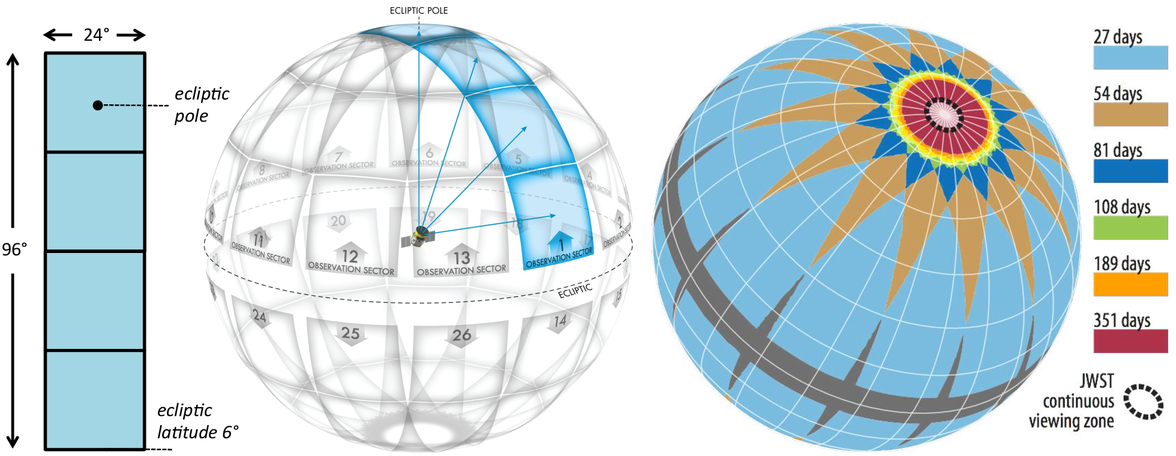
Figure 1: The observation strategy of TESS (Figure 7 from Ricker et al. (2014) licensed under CC BY 4.0). The left panel shows the field of view of a single TESS sector created by its four cameras. The middle panel shows how TESS divides and observes the sky in 26 partially overlapping sectors. The right panel shows how the overlap between sectors leads to certain ares of they sky being observed for longer durations.

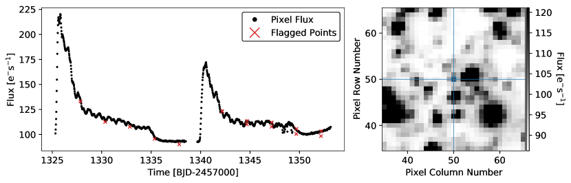
Figure 2: The systematic effects in the FFI data. In the left panel we show the Sector 1 raw light curve of the central pixel of the Type-Ia supernova ASASSN-18tb/SN 2018fhw. The sudden flux increases followed by a gradual decline at the beginning and middle of the light curve are caused by the scattered light from the Earth and Moon. The gap in the middle is when the data downlink occurred. The flagged points (red) indicate when the momentum dumps, a period of reduced pointing stability due to the spacecraft firing its thrusters, occurred. The high pointing jitter between 1348-1350 days was caused by an improper spacecraft configuration. In the right panel we show a $40\times 40$ pixel FFI cutout centered on ASASSN-18tb from Sector 1. The median value for each pixel is shown, and the color bar is calibrated to the 10-90% range of flux values. The central pixel of ASASSN-18tb is located where the two blue lines intersect and is surrounded by a blue square.

Similar to the Kepler spacecraft (Stumpe et al., 2012), some causes for these systematics include periods of reduced spacecraft pointing accuracy and changes in detector sensitivity due to temperature variations. dominant systematic effect for TESS is scattered light from the Earth and Moon entering the cameras and increasing the measured flux of a given pixel (Figure 2). This effect is caused by the spacecraft’s unique eccentric 13.7-day orbit, half the orbital period of the Moon, and usually occurs preceding or following a data downlink (which happens after each orbit) when the spacecraft is close to Earth.

Fortunately, many methods to remove systematics from light curves (i.e., “de-trending”) were developed during the Kepler/K2 era and serve as foundations for developing TESS de-trending methods. Correcting for systematics became particularly important during the K2 mission as the spacecraft was operating with reduced pointing accuracy compared to the original Kepler mission.

of these methods relied on the idea that flux variations that correlated with the source position on the CCD were likely to be systematic effects, an idea previously used to remove systematic effects in the photometric time series data from the Spitzer Space Telescope (Charbonneau et al., 2005; Knutson et al., 2008; Ballard et al., 2010; Stevenson et al., 2012). Using this “self-flat-fielding (SFF)” approach, Vanderburg & Johnson (2014), Armstrong et al. (2015), produced K2 light curves corrected for spacecraft motion, the dominant systematic effect. Aigrain et al. (2015, 2016) and Crossfield et al. (2015) modeled the spacecraft’s systematics as a Gaussian process, with pointing measurements as the input, and obtained de-trended light curves by subtracting the prediction of that model from the observed flux.

The unpopular package will complement existing open-source packages for extracting TESS FFI light curves. Two such popular packages are eleanor (Feinstein et al., 2019) and lightkurve (Barentsen et al., 2020).

This paper is organized as follows. In §2, we discuss the CPM method and the mathematical formulation behind the unpopular de-trending method. In §3, we describe the steps involved in creating light curves using the unpopular package and show an example of extracting a supernova light curve. In §4, we present de-trended FFI light curves. In §5, we discuss certain aspects of the method and summarize our work.

2 Causal Pixel Model

In this section we describe the concepts behind the CPM (and its variant CPM Difference Imaging) method and discuss the modifications we have made in our unpopular implementation. As mentioned in §1, CPM is within the family of methods that attempts to model the systematics as a combination of some chosen set of (e.g., Smith et al., 2012; Stumpe et al., 2012; Foreman-Mackey et al., 2015; Luger et al., 2016, 2018; Wang et al., 2016, 2017; Poleski et al., 2019).

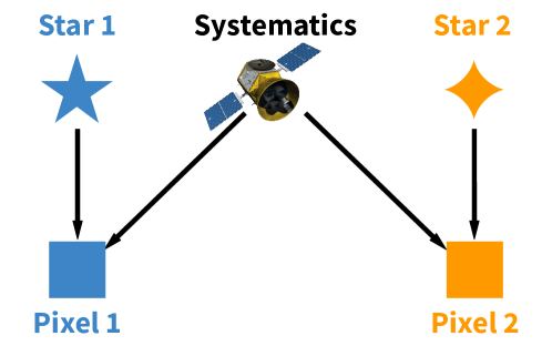
Figure 3: Diagram motivating the half-sibling regression method. The quantities in the top row (Star 1, Systematics, Star 2) are unobserved while the quantities in the bottom row (Pixel 1, Pixel 2) are observed. The two pixels are on the same CCD and separated by at least several times the size of the point spread function to ensure that no flux from one of the stars is simultaneously illuminating both pixels. Pixel 1 and Pixel 2 can be thought of as “half-siblings” as they both share a common parent (Systematics). TESS Spacecraft Image Credit: NASA’s Goddard Space Flight Center

While one key difference between them is the choice of regressors. In the official Kepler pipeline’s Presearch Data Conditioning module (PDC; Smith et al. 2012; Stumpe et al. 2012, 2014), the module responsible for correcting systematics, the regressors were the top eight “Cotrending Basis Vectors” (CBVs). The CBVs were different for each of the and they were obtained by performing Singular Value Decomposition (SVD) on a set of highly correlated and quiet light curves that were then ranked by their singular values. version 8.2 of the Kepler pipeline the above process is performed after first . For each of these time-series of a particular scale, an accompanying set of CBVs is generated and used as regressors in the de-trending step. Foreman-Mackey et al. (2015) took a similar approach by performing Principal Component Analysis (PCA) on a set of K2 Campaign 1 light curves and used the top 150 principal components, referred to as “eigen light curves”, as the regressors. EVEREST (Luger et al., 2016, 2018) uses products of the normalized pixel fluxes in a chosen K2 target’s aperture as the regressors . and the unpopular implementation use the light curves of many other pixels illuminated by distant sources on the same CCD as the regressors.

One subtle but significant aspect that sets CPM-based methods apart from the rest of these methods is that it works exclusively at the pixel level. Kepler PDC and Foreman-Mackey et al. (2015) work exclusively at the aperture photometry level, where both the quantity being modeled (i.e., the regressand) and the regressors are simple aperture photometry (SAP) light curves (technically the regressors are obtained by performing dimensionality reduction on SAP light curves). Aperture photometry is advantageous as individual pixel-level variations caused by systematics, such as pointing drift, can be significantly reduced by choosing an appropriately large aperture. However, particularly for TESS, where choosing a large aperture risks contamination from nearby sources given the relatively large pixels ($21$ arcseconds), working at the pixel level can yield better results. EVEREST incorporates pixel-level variations by generating the regressors from individual pixels’ flux measurements, although the regressand is still an SAP light curve. CPM-based methods go one step further where both the regressand and the regressors are individual pixel’s flux measurements. While a downside to this decision is that each pixel within an aperture must be separately, the computational efficiency of our implementation makes this problem tractable.

A significant concern for these linear models is the possibility of overfitting given their flexibility. That is, since we are fitting a linear combination of multiple regressors to a single time series (i.e., a pixel or aperture light curve), there is a possibility that the systematics model will not only capture the systematics but also variations from the astrophysical signal. One approach to mitigate overfitting is to reduce the flexibility of the model by using fewer regressors; this approach was adopted in the Kepler PDC module (Smith et al., 2012; Stumpe et al., 2012). Foreman-Mackey et al. (2015) prevents the systematics model from overfitting transits, the signal of interest in that study, by simultaneously fitting a transit model to the raw light curves. Another approach is regularization, in which an additional term is added to the objective function to control the behavior of the model and prevent overfitting; this approach was adopted in the CPM methods (Wang et al., 2016, 2017; Poleski et al., 2019). EVEREST 2.0 (Luger et al., 2018) combines both regularization and the simultaneous fitting of a Gaussian process to capture the astrophysical variability. The current approach in unpopular is somewhat similar to EVEREST 2.0 as we also use regularization and allow for simultaneous fitting with an additional model to capture astrophysical variability. However, instead of modeling the astrophysical variability with a Gaussian process as done in EVEREST 2.0, we use a simple polynomial model for computational efficiency.

Modifications to the original CPM method have been made in the unpopular implementation to reflect a change in the scientific objective. In the original CPM implementation, the objective was to detect exoplanet transits in the de-trended light curves. The model was tuned to specifically preserve transit signals, and the intrinsic stellar variability was removed by adding an autoregressive component. As the objective with unpopular is to obtain de-trended light curves for a variety of astrophysical sources, we prioritize preserving non-transit signals including stellar variability. Therefore, we autoregressive component and instead include the previously mentioned optional polynomial component.

2.1 Ordinary Least Squares

We will first write the mathematical formulation for the ordinary least squares (OLS) method. In the following subsection §2.2 we discuss ridge regression, an extension to OLS that incorporates regularization and is the method used in unpopular. We use the notation where lowercase upright fonts in bold ($\mathbf{y}$) are row or column vectors and uppercase upright fonts in bold ($\mathbf{X}$) are matrices.

2.2 Ridge Regression

As flexible linear models have a tendency to overfit, naively using the OLS method discussed above can result in the systematics model capturing most of the variations in the pixel being modeled, resulting in a de-trended pixel light curve that can resemble white noise. Overfitting can occur as the OLS method attempts to simply find the set of coefficients $\mathbf{\hat{w}}$ that minimizes the discrepancy between the model and data. We note that overfitting does not require that the predictors contain information about the (astrophysical) signal being fitted, and it thus also occurs in our setting where the predictors do not contain any information about the astrophysical signal of the target pixel. We therefore regularize our model to prevent overfitting.

Regularization allows us to prevent overfitting by adding an additional term, called the regularization or penalty term, to an objective function. In unpopular we use ridge regression (Hoerl & Kennard, 1970), which involves penalizing large (positive or negative) regression coefficients $w_{i}$ by adding a regularization term proportional to $\lVert\mathbf{w}\rVert_{2}^{2}=\sum_{i}w_{i}^{2}$, the square of the Euclidean ($L^{2}$) norm of $\mathbf{w}$, to the objective function $S(\mathbf{w})$. This penalization has the effect of shrinking the regression coefficients towards zero. Ridge regression is effective in alleviating issues related to having correlated regressors in a linear model (Hastie et al., 2001). The systematics model in unpopular contains many correlated regressors since pixels on a given TESS CCD share systematic trends. In addition, as shown below, ridge regression provides a closed-form expression for the ridge coefficients $\mathbf{\hat{w}_{\mathrm{ridge}}}$. Having a closed-form expression is attractive as it removes the need for iterative optimization algorithms and makes the method computationally efficient.

In the simplest case where all coefficients are equally penalized, the regularization term is $\lambda\lVert\mathbf{w}\rVert_{2}^{2}$ where $\lambda$ is a non-negative scalar that controls the penalization. A larger value of $\lambda$ results in stronger penalization (i.e., smaller regression coefficients). To equally penalize all the regressors, ridge regression is normally performed on normalized inputs (Hastie et al., 2001). We normalize both the regressand and the regressors by dividing by the median and subtracting 1. After de-trending, this process is inverted to return to the original units. For clarity, the normalized variables will be denoted with an asterisk ($*$) subscript (e.g., $\mathbf{y_{*}},\mathbf{X_{*}}$). After adding the regularization term, the modified objective function $S_{\mathrm{ridge}}(\mathbf{w})$ becomes

$$S_{\mathrm{ridge}}(\mathbf{w})=\mathbf{\lVert y_{*}-X_{*}\cdot w\rVert_{\mathrm{2}}^{\mathrm{2}}+\mathrm{\lambda}\lVert w\rVert_{\mathrm{2}}^{\mathrm{2}}}$$ (1)

and the ridge coefficients $\mathbf{\hat{w}_{\mathrm{ridge}}}$ are obtained by minimizing $S_{\mathrm{ridge}}(\mathbf{w})$. The formula to calculate $\mathbf{\hat{w}_{\mathrm{ridge}}}$ is

$$\mathbf{\hat{w}_{\mathrm{ridge}}}=(\mathbf{X_{*}^{\top}\cdot X_{*}}+\lambda\mathbf{I})^{-1}\cdot(\mathbf{X_{*}^{\top}\cdot y_{*}}),$$ (2)

where $\mathbf{I}$ is an identity matrix with the same dimensions as $(\mathbf{X_{*}^{\top}\cdot X_{*}})$.

We can generalize the above formulation to allow for separate specification of the penalization for each coefficient $w_{i}$. In other words, there can be a (possibly) different $\lambda_{i}$ for each $w_{i}$. For concreteness, we will assume the polynomial component is being used and that the size of $\mathbf{w}$ is . The generalization involves replacing the previous regularization parameter $\lambda$ with a matrix. We will denote this matrix as $\mathbf{\Gamma}$ and it will be an square and diagonal matrix

$$\mathbf{\Gamma}=\begin{bmatrix}\gamma_{1}&&\\ &\ddots&\\ &&\gamma_{\scriptscriptstyle{L+P+1}}\\ \end{bmatrix},$$ (3)

where each element $\gamma_{i}$ will turn out to be the square root of the regularization parameter $\lambda_{i}$. The term added to $S(\mathbf{w})$ $\mathbf{\lVert\Gamma\cdot w\rVert_{\mathrm{2}}^{\mathrm{2}}}$, and the modified objective function $S_{\mathrm{ridge}}(\mathbf{w})$ is

$$S_{\mathrm{ridge}}(\mathbf{w})=\mathbf{\lVert y_{*}-X_{*}\cdot w\rVert_{\mathrm{2}}^{\mathrm{2}}+\lVert\Gamma\cdot w\rVert_{\mathrm{2}}^{\mathrm{2}}}.$$ (4)

As shown in Appendix A.2, the coefficients $\mathbf{\hat{w}_{\mathrm{ridge}}}$ can be calculated with the formula

$$\mathbf{\hat{w}_{\mathrm{ridge}}}=(\mathbf{X_{*}^{\top}\cdot X_{*}}+\mathbf{\Gamma^{\top}\cdot\Gamma})^{-1}\cdot(\mathbf{X_{*}^{\top}\cdot y_{*}}).$$ (5)

We can rewrite this formula to more closely parallel Equation (2) by defining $\mathbf{\Lambda\equiv\Gamma^{\top}\cdot\Gamma}$ such that

$$\mathbf{\Lambda}=\begin{bmatrix}\lambda_{1}&&\\ &\ddots&\\ &&\lambda_{\scriptscriptstyle{L+P+1}}\\ \end{bmatrix},$$ (6)

where each element $\lambda_{i}=\gamma_{i}^{2}$. The formula for the coefficients $\mathbf{\hat{w}_{\mathrm{ridge}}}$ is then

$$\mathbf{\hat{w}_{\mathrm{ridge}}}=(\mathbf{X_{*}^{\top}\cdot X_{*}}+\mathbf{\Lambda})^{-1}\cdot(\mathbf{X_{*}^{\top}\cdot y_{*}}).$$ (7)

The simplest case of equal penalization is when $\lambda=\lambda_{i}$ and $\mathbf{\Lambda}=\lambda\mathbf{I}$.

In unpopular, we can currently specify up to two regularization parameters $\lambda_{\mathbf{L}}$ and $\lambda_{\mathbf{P}}$ depending on whether the coefficient is for a predictor pixel light curve (i.e., the systematics model) or for a polynomial component (i.e., astrophysical long-term trend). All the predictor pixel light curve regressors will be penalized with $\lambda_{\mathbf{L}}$, while the polynomial components will be penalized with $\lambda_{\mathbf{P}}$. The intercept term, , is left unpenalized (Hastie et al., 2001). The full regularization matrix $\mathbf{\Lambda}$ can be constructed as

$$\mathbf{\Lambda}=\begin{bmatrix}\mathbf{\Lambda_{\mathbf{L}}}&&\\ &\mathbf{\Lambda_{\mathbf{P}}}&\\ &&0\end{bmatrix},$$ (8)

where $\mathbf{\Lambda_{\mathbf{L}}}$ is an $L\times L$ square and diagonal matrix with all diagonal elements set to $\lambda_{\mathbf{L}}$ ($\mathbf{\Lambda_{L}=\lambda_{L}I}$), and $\mathbf{\Lambda_{\mathbf{P}}}$ is a square and diagonal matrix with all diagonal elements set to $\lambda_{\mathbf{P}}$ ($\mathbf{\Lambda_{P}=\lambda_{P}I}$). The final 0 value indicates that the intercept term is not regularized.

We now have a different set of coefficients $\mathbf{\hat{w}_{\mathrm{ridge}}}$ from using ridge regression instead of OLS. The rest of the approach is the same. The model is $\mathbf{\hat{m}=X_{*}\cdot\hat{w}_{\mathrm{ridge}}}$, and if the polynomial component was used, $\mathbf{\hat{m}}$ can be split up into the systematics component $\mathbf{\hat{m}_{\mathrm{sys}}}$, the astrophysical long-term component $\mathbf{\hat{m}_{\mathrm{poly}}}$, and the intercept term $\mathbf{\hat{m}_{\mathrm{offset}}}$ using Equations (LABEL:eqn:systematics_model), (LABEL:eqn:longterm_model), and (LABEL:eqn:offset). Similar to before, after subtracting $\mathbf{\hat{m}_{\mathrm{sys}}}$ from $\mathbf{y}_{*}$ to remove the systematics, the user can also subtract $\mathbf{\hat{m}_{\mathrm{poly}}}$ to remove any captured long-term trend and subtract $\mathbf{\hat{m}_{\mathrm{offset}}}$ to center the de-trended light curve around its average value.

2.3 Train-and-Test Framework

In unpopular we employ a modified version of the “train-and-test” framework used in the original CPM method (Wang et al., 2016) to further prevent overfitting.

Under this framework, the target pixel data used to calculate the coefficients $\mathbf{\hat{w}_{\mathrm{ridge}}}$, the training data, are from the target pixel data being predicted and de-trended, the test data. As the coefficients are calculated using the training data and the de-trending occurs on the test data, the model overfit signals with timescales shorter than the test data window. The separation is accomplished by splitting the target pixel light curve into $k$ contiguous sections .

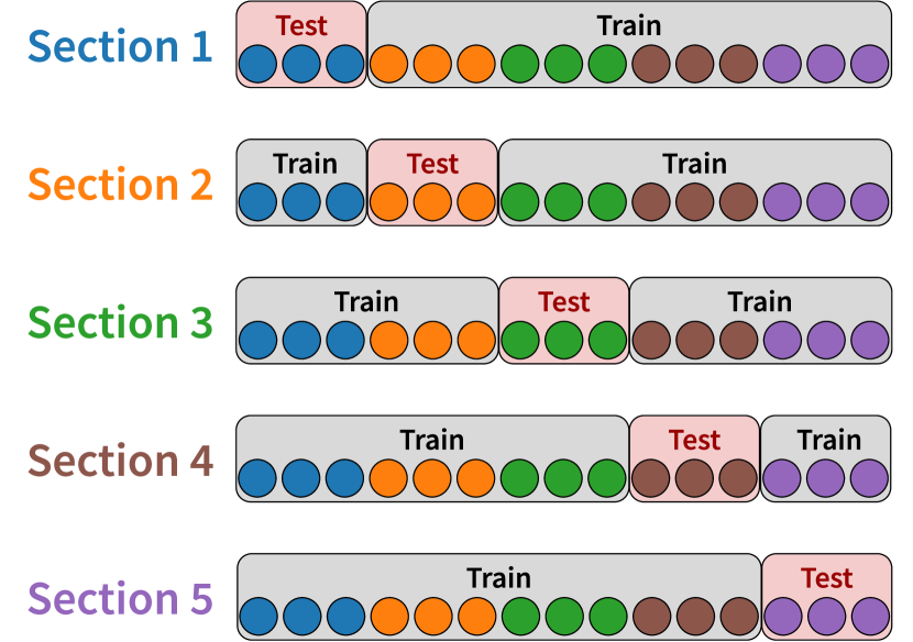
Figure 4: A diagram of the train-and-test framework. In this scenario, the light curve being de-trended is divided into five contiguous sections ($k=5$), each indicated by a separate color. For every test section being de-trended the model coefficients are obtained by fitting to the training data, which is the rest of the light curve. As $k$ is inversely proportional to the number of measurements in a given section, an appropriate choice for $k$ can be made is based on the timescale of the signal of interest.

3 Creating De-trended TESS light curves with unpopular

In this section we describe the steps for using unpopular to extract TESS FFI light curves. We will use the Sector 1 data for ASASSN-18tb/SN 2018fhw (Vallely et al., 2019), a Type-Ia supernova event observed by TESS, as an example. The coordinates for this source are RA, Dec (J2000): $64.525833^{\circ}$, $-63.615669^{\circ}$. While there are several tuning parameters (i.e., values and choices the user must make before de-trending) in these steps, we simply note the tuning parameters used for ASASSN-18tb during each of the steps and postpone discussing the effects of changing these parameters to §3.5.

3.1 Downloading Data

TESS obtains time-series photometry with its 16 CCDs (four CCDs per camera) in a given observing sector. Each CCD has $2048\times 2048$ science pixels, and the full FOV was recorded at either 30-minute cadence (Cycles 1 & 2) or 10-minute cadence (Cycle 3). The stack of all FFIs for a single CCD in a given sector taken with 30-minute cadence requires ${\sim}45$ GB of storage. As files of this size are not user-friendly and since unpopular only requires a region of the FFIs around a given source, we recommend downloading a cutout stack instead of a full FFI stack (see Figure 2). Calibrated FFI cutout stacks of a specified size centered at a given coordinate can be downloaded using tools such as TESScut (Brasseur et al., 2019) or lightkurve (Barentsen et al., 2020). The cutouts must be large enough to allow for enough predictor pixels to be chosen even when taking into account that a set of pixels close to the target pixel will be excluded. Based on our experience, we find that $100\times 100$ FFI cutouts (${\sim}250$ MB for a stack of 30-minute cadence FFIs) are reasonable for sources with aperture regions smaller than $5\times 5$ pixels. While we have not performed any tests, we do not believe our package is appropriate for obtaining light curves from saturated targets that illuminate a large region of the FFI cutouts. For users interested in saturated targets, the “halo-photometry” approach taken by White et al. (2017) and Pope et al. (2019) will likely be more successful.

3.2 Pre-processing

The TESS team provides QUALITY arrays that flag detected anomalies (e.g., spacecraft is in coarse point mode, reaction wheel desaturation event) in the data. The default behavior in unpopular is to remove the FFI cutouts with any quality flags prior to de-trending as they tend to be outliers (see Figure 2). The quality flags used here are those recorded in the FFI data, which are applicable to the entire CCD that the source was observed on.

After this step, unpopular calculates and stores the normalized version of the pixel light curves for all pixels in the FFI cutout. This step is necessary as, discussed in §2.2, ridge regression requires us to normalize both the regressand and the regressors. We divide each pixel light curve by its median value and then subtract 1 from the resulting light curve to center it around zero. This normalization makes the flux measurements unitless and we invert this process after de-trending to recover the physical units. We also allow the user to perform an initial background subtraction before de-trending, where we first obtain the median light curve of the 100 faintest pixels in the FFI cutout then subsequently subtract it from the entire cutout. While this initial background subtraction does not affect the shape of the de-trended light curve, it may rescale the light curve to a more accurate baseline flux level after de-trending. However, as we mention below the baselines fluxes are rough estimates and should not be treated as accurate. We did not perform the initial background subtraction for this example.

3.3 Model Specification

This step involves specifying the aperture, constructing the design matrix, and setting the regularization parameters.

3.3.1 Aperture Specification

While the method explained in §2 de-trends a single pixel light curve, for most scientific studies the user will want an aperture light curve. As unpopular produces a de-trended FFI cutout of a chosen rectangular set of pixels, the aperture light curve can be obtained by summing all the de-trended pixels or a subset of them. For every pixel being de-trended a separate linear model, each with its own set of predictor pixels and coefficients, is constructed. For ASASSN-18tb, we will use a $3\times 3$ square aperture covering rows 49 to 51 and columns 49 to 51, or in detector coordinates, rows 802 to 804 and columns 730 to 732 (Figure 5). The location of the source falls on pixel [50,50]. The $3\times 3$ aperture was chosen by visually inspecting the region around the source in the FFI cutout and by choosing an aperture that encompassed a set of contiguous pixels near the central pixel that were brighter than surrounding empty regions. While this approach is not quantitative nor easily programmable, developing a robust quantitative approach to automate aperture selection is beyond the scope of this work.

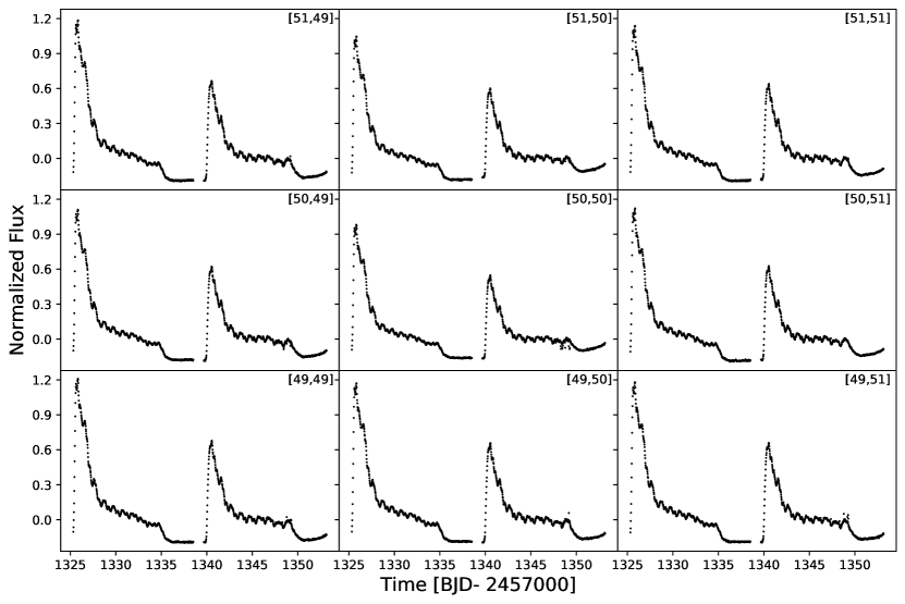
Figure 5: The normalized light curve for each pixel in the $3\times 3$ aperture of ASASSN-18tb. The numbers in the top right of each panel indicate the pixel row and column positions.

3.3.2 Constructing the Design Matrix

Constructing the design matrix consists of selecting the predictor pixels and deciding on whether to include or exclude the polynomial component. As predictor pixels must not be from the same source, we first set an exclusion region around each pixel where no predictor pixels are chosen from. The default exclusion region is an $11\times 11$ square set of pixels centered on each target pixel . For sources that do, the user will need to increase the size of the exclusion region.

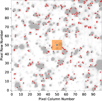
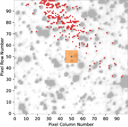
Figure 6: Difference between the choice of predictor pixels based on the selection method. In both panels, the pixel being de-trended is the central pixel (blue star). The exclusion region around the central pixel (shaded and hatched orange area) is where predictor pixels are not chosen from. In the left panel, the predictor pixels (red circles) were chosen based on having a similar median brightness to the pixel being de-trended. In the right panel, the predictor pixels were chosen based on having a high cosine similarity to the pixel being de-trended. The clustering of predictor pixels in the right panel indicates there are local systematic effects in this region.

Once the exclusion region is set we must decide on the number of predictor pixels $L$ and the method to choose them. While these decisions will be the same across all the pixels in the aperture, we reiterate that the set of chosen predictor pixels will be different for each target pixel. The number of predictor pixels must be large enough to allow for a flexible model that can capture most of the systematic effects. After experimentation, we found that the de-trending results were mostly similar for values of $L$ between 64–256. Setting $L$ below this range resulted in the de-trended light curve as the model was inflexible. Setting $L$ above this range increased the runtime (i.e., computational time) while showing similar de-trending results. chose $L=256$ predictor pixels as the default setting and find this value to be acceptable for many sources.

In Figure 6 we show two of the currently implemented methods for selecting the predictor pixels. In the left figure, the predictor pixels are the top $L=256$ pixels with the closest median brightness to the target pixel. This method is based on the idea that systematic effects may be more similar across pixels of similar brightness and is the default method. In the right figure, the predictor pixels are the top $L=256$ pixels with the highest cosine similarity (i.e., similar trend) to the target pixel. The fact that the predictor pixels are clustered in one area indicates that there are local systematic effects in this region. These local systematic effects, likely caused by the change in proximity of the spacecraft to Earth during an orbit, tend to “sweep” from one side of the FOV to the other. Although these “sweeping” signals create an opportunity to use time-lagged versions of pixel light curves as regressors, we postpone exploring this approach to a future study. While the set of predictor pixels are significantly different between these two methods, we found that the de-trending results were similar regardless of which method was chosen. We also found that randomly choosing the predictor pixels worked as well as the other methods. For ASASSN-18tb, we used the default settings for both the number and selection method of the predictor pixels.

The final step in constructing the design matrix is choosing whether to include or exclude the polynomial component. A single polynomial is used for the whole Sector of data. When the source is expected to show long-term astrophysical trends, such as a supernovae or other explosive transients, including the polynomial component mitigates distorting the de-trended light curve. Erroneously excluding the polynomial component when there is long-term astrophysical variability will likely result in a reduction of the amplitude of the long-term signal and distortions in other parts of the light curve as the systematics model will attempt to fit to the astrophysical signal. If the user chooses to include a polynomial component, the default setting creates a cubic polynomial . As the polynomial is simply there to capture long-term astrophysical trends, in general we do not recommend the use of more flexible higher degree polynomials. For this example we included the default cubic polynomial.

3.3.3 Setting the Regularization Parameters

After the design matrix has been constructed, the regularization parameters must be set. The regularization parameters are set separately for the systematics model $\lambda_{\mathbf{L}}$ and the polynomial model $\lambda_{\mathbf{P}}$ (if using). As mentioned in §2, the regularization parameters are defined as the precision, the reciprocal of the variance, of the Gaussian prior for each regressor. Therefore, larger values of $\lambda$ lead to stronger regularization. For ASASSN-18tb, we set $\lambda_{\mathbf{L}}=0.01$ and $\lambda_{\mathbf{P}}=0.01$. The effects of changing these values are discussed in §3.5.

3.4 De-trending

The final tuning parameter to set before de-trending is $k$, the number of sections to use for the train-and-test framework (see §2.3). The smallest possible choice is $k=2$, which separates the light curves into two sections. The largest possible choice is when $k$ is equal to the number of data points, where a separate set of coefficients $\mathbf{\hat{w}_{\mathrm{ridge}}}$ is calculated to predict each data point. We set $k=126$ (approximately ten data points for each section) for ASASSN-18tb. We de-trend each pixel inside the aperture by fitting the linear model defined in §2 and subtracting the systematics component. The de-trending took ${\sim}5$ seconds on a Dell XPS 15 9570 laptop (Intel Core i7-8750H 2.20 GHz) and we show the results in Figure 7. The top plot shows each of the de-trended pixel light curves and the bottom plot shows the aperture light curve. We obtain the aperture light curve by summing all the rescaled de-trended pixel light curves. The rescaling is done by inverting the normalization, or in other words by multiplying each de-trended pixel light curve by its original median value and then adding back the median value. We caution the user that we do not expect adding the median flux will shift the de-trended light curve to the “true” flux level. Shifting the de-trended light curve to an accurate flux level will likely require comparing the de-trended light curve to a known comparison object in the FOV (i.e., relative photometry) and is beyond the scope of this project. Our aperture de-trended light curve is similar to that obtained by Vallely et al. (2019), where they used the ISIS image subtraction package (Alard & Lupton, 1998; Alard, 2000).

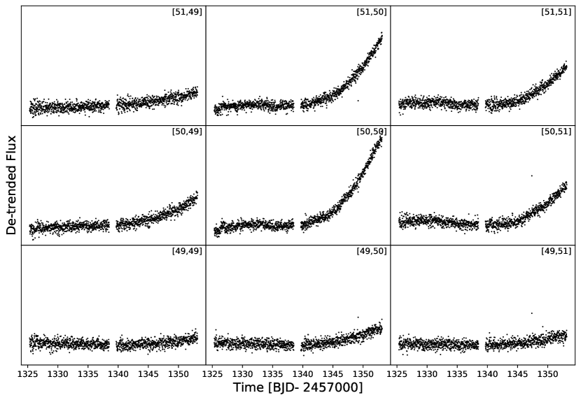
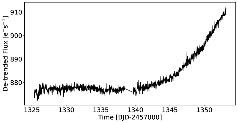
Figure 7: The de-trended pixel light curves (top panel) and the de-trended aperture light curve (bottom panel). Each of the light curves in the top panel are the de-trended versions of those shown in Figure 5. The aperture light curve is obtained by first scaling each pixel light curve to its estimated physical flux and then summing them together. No initial background subtraction was performed, a cubic polynomial was added to capture the long-term trend, and we set $L=256,\lambda_{\mathbf{L}}=0.01,\lambda_{\mathbf{P}}=0.01,k=126$.

3.5 Tuning Parameters

We discuss the effects of modifying the tuning parameters (i.e., hyperparameters) here. We restrict the discussion to three tuning parameters: the regularization parameters $\lambda_{\mathbf{L}}$ and $\lambda_{\mathbf{P}}$, and the number of sections $k$ for the train-and-test framework. We will use ASASSN-18tb’s central pixel ($[50,50]$), the pixel with the largest variation after de-trending (see Figure 7), to demonstrate the effect of changing the tuning parameters.

To quantify the effects of changing these tuning parameters, we calculated a proxy for the 6-hr combined differential photometric precision (CDPP) (Christiansen et al., 2012) on the de-trended pixel light curve. CDPP is a photometric noise metric in units of parts-per-million (ppm) developed by the Kepler team to define the ease of detecting a weak terrestrial transit signature at a given timescale in a light curve. A smaller value is preferred as CDPP is a characterization of the noise. The proxy we use for the 6-hr CDPP, based on the approach by Gilliland et al. (2011), is easier to calculate than the formal wavelet-based CDPP and is implemented in the lightkurve package. The method first fits and subtracts a running 2-day quadratic polynomial (i.e., Savitzky–Golay filter) from the de-trended light curve to remove low-frequency signals. After this step, sigma-clipping at $5\sigma$ is done to remove outliers. The proxy CDPP is then calculated as the standard deviation of the 6-hr (12 measurements with 30-minute cadence data) running mean. We refer to this value as the 6-hr CDPP hereafter.

While we calculate CDPP, we note that for the example source, which is a supernova, CDPP is not a particularly good metric to assess the quality of the de-trended light curve. CDPP was developed for assessing the ease of detecting Earth-like transit signatures and is the appropriate metric to optimize when de-trending light curves for exoplanet searches. For users interested in obtaining supernova light curves, stellar rotation periods, or investigating stellar variability in general, de-trending based on minimizing CDPP risks removing signals of interest. However, as we find that smaller values of CDPP tend to go hand in hand with qualitatively good light curves, we use CDPP for demonstrative purposes. While there exist other metrics developed with studying stellar variability in mind (Basri et al., 2013) we defer investigating these metrics to a future paper.

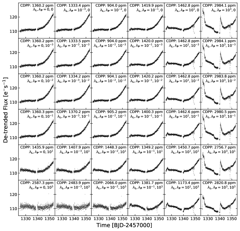
Figure 8: Different de-trending results for the central pixel of ASASSN-18tb when varying $\lambda_{\mathbf{L}}$ and $\lambda_{\mathbf{P}}$ while fixing $L=256,k=126$. Each panel shows the de-trended pixel light curve and the 6-hr CDPP for a specific combination of $\lambda_{\mathbf{L}}$ and $\lambda_{\mathbf{P}}$. The value of $\lambda_{\mathbf{L}}$ increases from the left column to the right column, and the value of $\lambda_{\mathbf{P}}$ increases from the top row to the bottom row. The smallest 6-hr CDPP values of ${\sim}904$ ppm are obtained in the top four rows of the third column where $\lambda_{\mathbf{L}}=10^{-2}$ and $\lambda_{\mathbf{P}}=0,10^{-3},10^{-2},10^{-1}$. The bottom-left panels show signs of the systematic component overfitting to the long-term trend, while the right columns show signs of underfitting

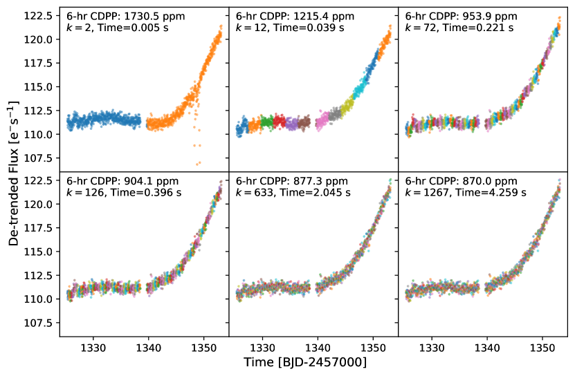
Figure 9: Different de-trending results for the central pixel of ASASSN-18tb when varying $k$, the number of sections to use for the train-and-test framework. Other tuning parameters were kept constant ($L=256,\lambda_{\mathbf{L}}=\lambda_{\mathbf{P}}=10^{-2}$). Each section is indicated by points of the same color (non-contiguous points of the same color are different sections). As $k$ becomes larger, the 6-hr CDPP decreases while the runtime increases. While most values of $k$ show similar results, when $k=2$ the systematic effects around 1348-1350 days are still present in the de-trended light curve.

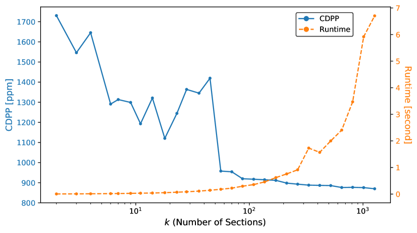
Figure 10: The 6-hr CDPP and runtime for de-trending the central pixel of ASSASSN-18tb as a function of $k$ ($L=256,\lambda_{\mathbf{L}}=\lambda_{\mathbf{P}}=10^{-2}$). Note that the x-axis is scaled logarithmically. The 6-hr CDPP fluctuates while decreasing until around $k{\sim}45$ and then shows a significant decrease beyond that point. It then shows marginal decreases from $k{\sim}100$ while the runtime increases roughly linearly.

In Figure 8 we show the effect of changing the regularization parameters by running the de-trending method on a coarse grid of $\lambda_{\mathbf{L}}$ and $\lambda_{\mathbf{P}}$ and calculating the 6-hr CDPP. Each panel shows the same de-trended pixel light curve, the central pixel for ASASSN-18tb, and the 6-hr CDPP for a different combination of $\lambda_{\mathbf{L}}$ and $\lambda_{\mathbf{P}}$ while we kept the other values constant ($L=256,k=126$). The values that both $\lambda_{\mathbf{L}}$ and $\lambda_{\mathbf{P}}$ can take are $[0,\;10^{-3},\;10^{-2},\;10^{-1},\;10^{1},\;10^{3}]$. The values of $\lambda_{\mathbf{L}}$ are in increasing order from the most left column ($\lambda_{\mathbf{L}}=0$) to the most right column ($\lambda_{\mathbf{L}}=10^{3}$). The values of $\lambda_{\mathbf{P}}$ are in increasing order from the top row ($\lambda_{\mathbf{P}}=0$) to the bottom row ($\lambda_{\mathbf{P}}=10^{3}$). In other words, the regularization increases the further right or down the panel is. Looking at the two most right columns, particularly the most right column, we see that more of the systematic effects remain in the de-trended light curve. This behavior is due to the large value of $\lambda_{\mathbf{L}}$ causing the systematics model to be rigid and therefore underfit. In the lower rows where $\lambda_{\mathbf{P}}$ is large we see that the polynomial model is underfitting and either the systematics model overfits and removes the long-term trend (in the left columns) or the systematics model also underfits and the de-trended light curve looks similar to the original light curve (in the right columns). The smallest values for the 6-hr CDPP are obtained in the third column ($\lambda_{\mathbf{L}}=10^{-2}$) where it is ${\sim}904\,\mathrm{ppm}$ in the top four rows. We see that for each of the columns the top four rows show essentially the same results both in terms of the shape of the de-trended light curve and the 6-hr CDPP, indicating that the results are not particularly sensitive to the choice of $\lambda_{\mathbf{P}}$ and that there is a range of “good” values (spanning several orders of magnitude) when using a cubic polynomial. We further investigated this behavior by experimenting with higher degree polynomials such as a 13th-degree polynomial and a 50th-degree polynomial, and found that the results become more sensitive to the value of $\lambda_{\mathbf{P}}$ as these flexible polynomials start to capture the same variations as the systematic model when not sufficiently regularized.

In Figure 9 and 10 we show the effect of changing $k$, the number of sections to use for the train-and-test framework . As explained in §2.3, each section of the light curve is de-trended using the coefficients obtained from fitting to the of the light curve. The smallest possible value is $k=2$ and the largest possible value is when $k$ is equal to the number of data points. Figure 9 shows the de-trended pixel light curve and the calculated 6-hr CDPP for several different values of $k$. We see that the 6-hr CDPP decreases as we increase $k$ but at the cost of a higher runtime. To further investigate this relationship, we plotted the 6-hr CDPP and the runtime for a given value of $k$ in Figure 10. The 6-hr CDPP fluctuates while decreasing until around $k{\sim}45$ and then shows a significant decrease beyond that point. It then shows marginal decreases from $k{\sim}100$ while the runtime increases roughly linearly. This behavior shows that setting $k$ in the ${\sim}100{-}200$ range is a good trade-off between minimizing the CDPP and the runtime. In general, we believe that this range will be appropriate for most use cases. However, we also recommend the user try a range of values to check for any significant differences between the de-trended light curves. Additionally, for Cycle 3 and beyond where the FFIs will be taken at 10-minute cadence, the value of $k$ will likely need to be increased.

4 Additional Examples & Discussion

In this section we show and discuss additional de-trending results for several sources: the tidal disruption event ASASSN-19bt (Holoien et al., 2019), an exoplanet-hosting star TOI-172 (TIC 29857954) (Rodriguez et al., 2019), and a fast-rotating variable star (TIC 395130640). When appropriate, we compare our method to other de-trending pipelines.

4.1 TDE ASASSN-19bt

Tidal disruption events (TDEs) occur when a star passes sufficiently close to a supermassive black hole and is torn apart by the black hole’s tidal forces. As some of the star’s mass form an accretion disk around the black hole, it produces an observable bright flare. ASASSN-19bt/AT 2019ahk, initially discovered by the ASAS-SN project in January 2019 , was a TDE observed by TESS in its southern Continuous Viewing Zone (CVZ) (Stanek, 2019; Holoien et al., 2019). The CVZ is a ${\sim}12^{\circ}$ radius circular region of the sky centered at the ecliptic pole, in this case the southern ecliptic pole, that TESS observes for roughly a full year (one Cycle). As a source located at RA, Dec (J2000): $105.04811^{\circ},-66.04004^{\circ}$ in the southern CVZ, ASASSN-19bt was observed between Sectors 1-13 excluding Sector 6 where the source fell on a chip gap. The TDE was first observed in the second orbit of Sector 7.

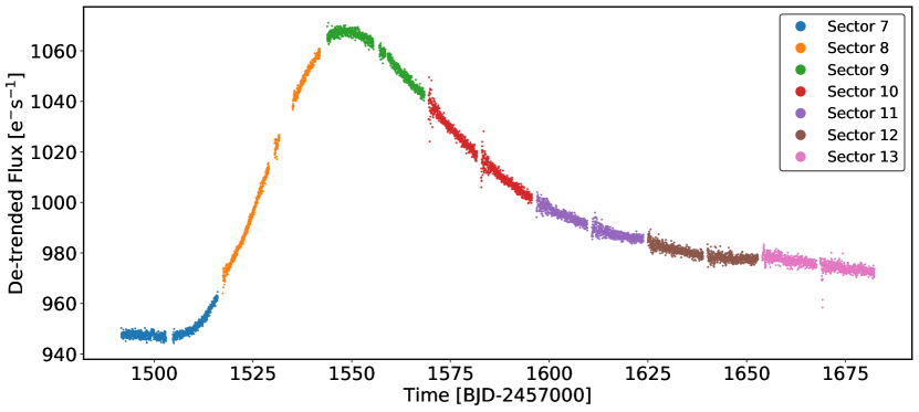
Figure 11: The multi-sector de-trended light curve of the tidal disruption event ASASSN-19bt. Each sector was de-trended separately and the de-trended light curves were stitched together as described in the text. For each sector we chose a $3\times 3$ aperture centered on the source, did not perform an initial background subtraction, added a cubic polynomial, and set $L=256,\lambda_{\mathbf{L}}=\lambda_{\mathbf{P}}=0.01,k=150$.

In 11 we show the results of de-trending Sectors 7-13, which is when the TDE occurred. Data from each sector was de-trended separately as the locations of the predictors pixels are not consistent across sectors. We did not perform the initial background subtraction for this source. For each sector we chose a $3\times 3$ aperture centered on the source, added a cubic polynomial, and used $L=256,\lambda_{\mathbf{L}}=\lambda_{\mathbf{P}}=0.01,k=150$ in the de-trending step. To correct for these offsets we first take the last 100 points from the Sector 7 light curve and the first 100 points from the Sector 8 light curve simultaneously fit for the slope and the two average values of these two portions, and then shift the Sector 8 light curve by adding the linear offset and the difference of the two means. This correction therefore shifts the Sector 8 light curve relative to the Sector 7 light curve. After the Sector 7 and Sector 8 are stitched together, we repeat this process with the partially stitched light curve and the remaining sectors’ light curves until all sectors are stitched together. While this stitching is currently implemented in the package, it is not ideal as this simple linear model is unable to capture any non-linear offsets. However, as stitching light curves is a separate problem, it is beyond the scope of this project to optimize this process. The de-trended light curves from Sectors 7-9 are comparable to those shown in Holoien et al. (2019), where they used the ISIS image subtraction package (Alard & Lupton, 1998; Alard, 2000) to create difference light curves for these three sectors. To our knowledge, our study is the first time the de-trended light curves have been presented for Sectors 10-13.

4.2 TOI-172

TOI-172 (TIC 29857954) is a slightly evolved G star hosting a hot Jupiter exoplanet (TOI-172 b) with a 9.48-day orbital period (Rodriguez et al., 2019). As the star was not pre-selected as a 2-minute cadence target, TOI-172 b was the first confirmed exoplanet in the TESS FFI data (Rodriguez et al., 2019).

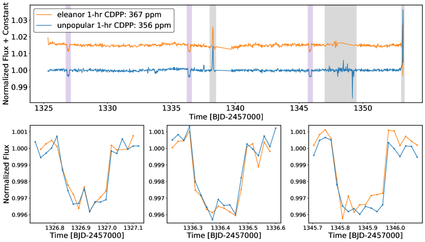
Figure 12: A comparison of de-trending results between the eleanor and unpopular packages. In the top panel we show the two de-trended light curves. Similar to Feinstein et al. (2019), we remove the three transit signals (purple shaded regions) and three specific periods (gray shaded regions), before calculating the 1-hr CDPP using the lightkurve package. The first region is when an asteroid crossed the aperture, the second region is when an improper spacecraft configuration caused high pointing jitter, and the third region is when scattered light from the Moon caused large spikes. The unpopular light curve has a lower 1-hr CDPP of 356 ppm. To obtain the unpopular light curve, we chose a $3\times 3$ aperture centered on the source, did not add a polynomial component, performed the initial background subtraction, and set $L=256,\lambda_{\mathbf{L}}=0.01,k=150$. In the bottom three panels we show the de-trended light curves around the three transit signals. The transit depths are comparable between the two light curves.

While unpopular was not optimized to obtain light curves with transit signals, we tested our de-trending method on Sector 1 data and present our results in Figure 12. We chose a $3\times 3$ aperture centered on the source, did not add a polynomial component, performed the initial background subtraction, and used $L=256,\lambda_{\mathbf{L}}=0.01,k=150$ in our de-trending step. The initial background subtraction was necessary to prevent the transits from becoming shallower in the normalized flux space. After identifying the times where transits occurred, in this case by finding the outliers to the running average of the de-trended light curve, we masked these transits and reran the de-trending step on the original data. This “masking” approach of removing transits during the de-trending step can prevent our misspecified model from erroneously fitting to the transit signals and distorting them. This approach is explained in detail in Section 4.1 of Luger et al. (2016). While the difference was negligible for this source, for light curves containing large signals (e.g., deep transits, eclipsing binaries, flares, microlensing events) this approach will likely result in substantial improvement. An alternative but computationally expensive approach to prevent distorting the transit signal, used in Foreman-Mackey et al. (2015), is to fit a joint transit and systematics model.

In the top panel of Figure 12 we also show the corrected light curve obtained using the eleanor package (Feinstein et al., 2019). Following a similar approach to Feinstein et al. (2019), we calculated the 1-hr CDPP for each light curve after removing the transits and specific excluded periods. The first excluded period $(1338<\mathrm{Time}<1338.5)$ is when an asteroid crossed the aperture (Rodriguez et al., 2019), the second excluded period $(1347<\mathrm{Time}<1349.5)$ is when the spacecraft experienced high pointing jitter due to an improper configuration, and the third excluded period $(\mathrm{Time}>1353)$ is when the scattered light from the Moon entered the FOV. The eleanor 1-hr CDPP is 367 ppm and the unpopular 1-hr CDPP is 356 ppm. This minor difference in the CDPP should not be viewed as unpopular outperforming eleanor given how various choices during the de-trending step can easily change the CDPP. In the bottom three panels, we show the de-trended light curves around the three transit signals. The overall shape and the depth between the two light curves is comparable. We note that the initial background subtraction was necessary to recover this transit depth. Omitting the initial background subtraction resulted in shallower transits as the estimated baseline flux was higher, resulting in suppressed depths in the normalized flux space. The comparable performance of to the eleanor package shows that with similar CDPP and recovered transit depths to the eleanor package, this result indicates that unpopular can also be used for studying exoplanets with comparable performance to other packages optimized for exoplanet searches.

4.3 TIC 395130640

Figure 13: Analysis of Sector 11 TIC 39513064 data. In the top panel we show the background-subtracted and normalized FFI data (black), the systematics prediction from the unpopular package (red), and the de-trended light curve (blue) centered around zero. The two dips at the beginning of each orbit are due to the initial background subtraction overcorrecting the scattered light signal. In the center panel we show the SPOC 2-minute light curve binned to 30 minutes (orange) and the de-trended unpopular FFI light curve (blue). Two regions of strong scattered light at the beginning of each orbit were removed in the SPOC light curve as it affected the SPOC pipeline’s systematics removal process. In the bottom-left panel we plot the Lomb-Scargle periodograms for these two light curves, showing that they both peak at 0.413 days. We folded both light curves with this period and show them in the bottom-right panel. To obtain the unpopular light curve, we used the SPOC aperture, performed an initial background subtraction, did not add a polynomial component, and set $L=256,\lambda_{\mathbf{L}}=1,k=150$.

TIC 395130640 (2MASS J11165730-8027522) is an M dwarf with $M=0.137\;M_{\odot},R=0.179\;R_{\odot}$, and a measured rotation period of $P=0.413\;\mathrm{days}$ (Newton et al., 2018). TIC 395130640 was observed in Sectors 11 & 12, and as a source in the TESS Candidate Target List has 2-minute cadence data de-trended by the SPOC pipeline (Jenkins et al., 2016) We chose to demonstrate our package’s performance on this source simply because it allows us to compare our performance to the official SPOC pipeline and also to verify that we can recover the same rotation period as the previously published value.

Prior to de-trending the Sector 11 FFI data we performed the initial background subtraction as we saw that that the FFI flux values were ${\sim}30\%$ higher than the values for large sections of the light curve. After this subtraction the FFI values were only ${\sim}6\%$ higher. Investigating the cause of this difference is beyond the scope of this paper, but it is likely a product of how the SPOC pipeline calibrates the FFI data and TPF data differently. It is possible that this issue can be attributed to the known issue where the SPOC pipeline can overestimate the background flux level and artificially lower the baseline flux level. (Kostov et al., 2020; Feinstein et al., 2020; Burt et al., 2020)

After this initial background subtraction, we de-trended the Sector 11 FFI data with the same aperture as the SPOC pipeline, did not add a polynomial component, and used $L=256,\lambda_{\mathbf{L}}=1,k=150$ in our de-trending step. . Note that in this case, as our model does not have a sinusoidal component, there is significant misspecification, and regularizing the systematics component more strongly was beneficial.

In the top panel of Figure 13 we show the background-subtracted and normalized FFI data, the prediction from the systematics model, and the de-trended light curve obtained by subtracting the systematics model from the normalized FFI data. These light curves are centered about zero as they have not been rescaled to the original flux levels. The two large dips at the beginning of each orbit in the FFI data are due to the initial background subtraction overcorrecting the scattered light signal. In the center panel we show the median-normalized SPOC 2-minute light curve binned to 30 minutes, to match the cadence of the FFI data, and the median-normalized de-trended unpopular FFI light curve. While the two regions at the beginning of each orbit were removed in the 2-minute data as the strong scattered light from the Earth affected the SPOC pipeline’s systematics removal step, our method was able to de-trend those regions. The unpopular light curve and the binned SPOC light curve show marginal differences besides the smaller amplitude of variability in the unpopular light curve. We believe this amplitude difference is a result of the additional corrections being applied in the PDC module of the SPOC pipeline, as we saw that the amplitudes between the SPOC SAP and the unpopular light curves were similar. While we checked to see whether the difference between the SAP and the PDCSAP flux could be explained by the CROWDSAP value, the ratio of target flux to total flux in the optimal aperture, the differences were still present after multiplying the CROWDSAP value to the PDCSAP flux value. Regardless of the origin of this discrepancy, as PDCSAP light curves are the standard we opt to compare our light curve to those. We used the lightkurve package to identify the periods of the two light curves using the Lomb-Scargle periodogram (Lomb, 1976; Scargle, 1982; VanderPlas, 2018). The periodograms are shown in the bottom-left panel of Figure 13. The maximum power, the semi-amplitude of the oscillation, for the binned SPOC light curve is 0.0128 while it is 0.0107 for the unpopular light curve. The period at maximum power for both light curves is $P=0.413\;\mathrm{days}$ and is in agreement with the previously published value (Newton et al., 2018). We folded both light curve with this period of 0.413 days and show them in the bottom-right panel. These results indicate that our lightweight method will allow users to efficiently produce de-trended FFI light curves of comparable quality to the 2-minute light curves produced by the SPOC pipeline.

5 Discussion & Conclusion

We have presented unpopular, an open-source Python package to efficiently extract de-trended light curves from TESS FFIs. The unpopular package is based on the CPM methods, originally developed for Kepler and K2 data (Wang et al., 2016, 2017), and employs regularized linear regression (i.e., ridge regression) to de-trend individual pixel light curves. Using the realization that pixels illuminated by different sources on the same CCD are likely to share similar systematic effects but unlikely to share similar astrophysical trends, the regressors for this data-driven linear model are pixel light curves from other distant (and thus causally disconnected) sources in the image. To prevent overfitting, we incorporated $L_{2}$ regularization and a train-and-test framework where the data points used to obtain the model coefficients and the data points being de-trended are mutually exclusive. We also allow for adding an additional polynomial component in the model to capture and preserve any long-term trends that may be astrophysical in the data. As the model is linear, de-trending takes only a few seconds for a given source.

We validated our method by de-trending a variety of sources and comparing them to those obtained by other pipelines. Our de-trended light curves for the supernova ASASSN-18tb and the TDE ASASSN-19bt are similar to the published light curves (ASASSN-18tb: Vallely et al. (2019), ASASSN-19bt: Holoien et al. (2019)), where they used the ISIS image subtraction package. We show the de-trended light curves for Sectors 7-13 of ASASSN-19bt, where light curves for Sectors 10-13 have not been published before. For TOI-172, an exoplanet-hosting star, we compared our light curve to that obtained by the eleanor package. Our package was able to recover the transits and also produce a light curve with a lower CDPP than eleanor, indicating that our package can also be used for exoplanet studies. For TIC 395130640, a fast-rotating M dwarf, we compared our FFI light curve to the 2-minute light curve de-trended by the SPOC pipeline. Other than a slightly decreased amplitude in the variation, our light curve shows the same structure as the SPOC light curve, indicating that our lightweight package can produce light curves with similar quality to the SPOC pipeline. Additionally, our package was able to de-trend regions of strong scattered light that the SPOC pipeline was not able to.

While we have presented favorable results, as with any method there are limitations to our approach. One limitation is the lack of an automated method to choose the optimal set of parameters for the de-trending process: the number of predictor pixels $L$, the selection method for choosing the set of predictor pixels, the decision of whether to incorporate a polynomial component, the degree of the polynomial, the regularization parameters $\lambda_{\mathbf{L}},\lambda_{\mathbf{P}}$, and the number of sections to use for the train-and-test framework $k$. While one could in principle make these choices based on minimizing the CDPP, this approach is only appropriate for users interested in exoplanets. For other sources, the user will have to make some of these choices based on the signal they are interested in, such as how the inclusion of the polynomial component and its degree is based on whether the user is attempting to recover sources that contain long-term astrophysical trends (e.g., supernovae, tidal disruption events, slow-rotating stars). Other choices can be made heuristically, such as how the value of $\lambda_{\mathbf{L}}$, as also mentioned in §4.3, will likely need to become larger the more the model is a misspecification for the underlying data. For the examples given in this paper, we chose the values based on visual inspection of the de-trended light curve. Visual inspection is reasonable for sources that already have published light curves, but is impractical for blind searches as the number of light curves will be large. Overcoming this limitation will likely require the development of various light curve “goodness” metrics that can be optimized for different types of sources.

Another limitation is the use of the polynomial component for capturing trends in the data. While the polynomial is effective at capturing certain long-term trends, it is neither physically motivated nor appropriate for certain variations. For example, the sinusoidal variation of TIC 395130640 cannot be captured with a low-degree polynomial. A sufficiently high-degree polynomial could potentially capture the variation but would also likely start fitting to the systematic effects. One approach, used in Angus et al. (2016) and Hedges et al. (2020) is to explicitly include a sinusoidal component and simultaneously fit the systematic effects and periodic variations over a grid of frequencies. Another slightly more general approach, employed in the EVEREST and EVEREST 2.0 pipelines, is to replace the polynomial component with a Gaussian process. While both approaches are more computationally expensive, there will likely be improvements depending on the source.

While the method takes only a few seconds to de-trend a given source, we could still reduce the computational time by parallelizing the code. As each pixel is de-trended independently, parallelizing the code is conceptually straightforward. Significantly reducing the computational time of this method could allow for the production of high-level science products where we de-trend every pixel in the TESS FFIs. These de-trended FFIs could be helpful for detecting both transient events and moving sources in an FFI.

The code is open source under the MIT license and available at https://github.com/soichiro-hattori/unpopular along with a Jupyter notebook tutorial. We hope that this method and the techniques used here can be generalized and applied to upcoming missions such as PLATO (Rauer et al., 2014) and the LSST survey at the Vera C. Rubin Observatory (Ivezić et al., 2019) in removing systematic effects to make new discoveries.

Appendix A Solutions to Linear Least Squares

Consistent with the notation in §2, lowercase upright fonts in bold ($\mathbf{y}$) are row or column vectors and uppercase upright fonts in bold ($\mathbf{X}$) are matrices.

A.1 Ordinary Least Squares

Here we derive the set of coefficients $\mathbf{\hat{w}}$ that minimizes the sum of squared residuals

$$S(\mathbf{w})=\mathbf{\lVert y-X\cdot w\rVert_{\mathrm{2}}^{\mathrm{2}}=(y-X\cdot w)^{\top}\cdot(y-X\cdot w)}.$$ (A1)

Expanding this expression gives

$$S(\mathbf{w}) =\mathbf{(y-X\cdot w)^{\top}\cdot(y-X\cdot w)}$$ (A2)

$$=\mathbf{(y^{\top}-w^{\top}\cdot X^{\top})\cdot(y-X\cdot w)}$$ (A3)

$$=\mathbf{(y^{\top}\cdot y)-(y^{\top}\cdot X\cdot w)-(w^{\top}\cdot X^{\top}\cdot y)+(w^{\top}\cdot X^{\top}\cdot X\cdot w)}$$ (A4)

$$S(\mathbf{w}) =\mathbf{(y^{\top}\cdot y)-\mathrm{2}(w^{\top}\cdot X^{\top}\cdot y)+(w^{\top}\cdot X^{\top}\cdot X\cdot w)}$$ (A5)

where we use $\mathbf{y^{\top}\cdot X\cdot w=(y^{\top}\cdot X\cdot w)^{\top}=w^{\top}\cdot X^{\top}\cdot y}$ as it is a scalar. To find the $\mathbf{w}$ that minimizes $S(\mathbf{w})$, we take the derivative of $S(\mathbf{w})$ with respect to $\mathbf{w}$ and set it to zero. Using the denominator layout convention for matrix differentiation,

$$\frac{\partial S(\mathbf{w})}{\partial\mathbf{w}} =\mathbf{\frac{\partial}{\partial w}(y^{\top}\cdot y)-\mathrm{2}\frac{\partial}{\partial w}(w^{\top}\cdot X^{\top}\cdot y)+\frac{\partial}{\partial w}(w^{\top}\cdot X^{\top}\cdot X\cdot w)}$$ (A6)

$$=\mathbf{\mathrm{0}-\mathrm{2}(X^{\top}\cdot y)+\mathrm{2}(X^{\top}\cdot X\cdot w)}$$ (A7)

$$\frac{\partial S(\mathbf{w})}{\partial\mathbf{w}} =\mathbf{\mathrm{2}(X^{\top}\cdot X\cdot w)-\mathrm{2}(X^{\top}\cdot y)=\mathrm{0}\Rightarrow X^{\top}\cdot X\cdot w=X^{\top}\cdot y}.$$ (A8)

If $(\mathbf{X^{\top}\cdot X})$ is an invertible square matrix, we can left multiply $(\mathbf{X^{\top}\cdot X})^{-1}$ to both sides of the above expression to solve for $\mathbf{\hat{w}}$

$$\mathbf{\hat{w}=(X^{\top}\cdot X)^{-1}\cdot(X^{\top}\cdot y)}.$$ (A9)

A.2 Ridge Regression

Here we derive the ridge coefficients $\mathbf{\hat{w}_{\mathrm{ridge}}}$ that minimize the objective function

$$S_{\mathrm{ridge}}(\mathbf{w})=\mathbf{\lVert y_{*}-X_{*}\cdot w\rVert_{\mathrm{2}}^{\mathrm{2}}+\lVert\Gamma\cdot w\rVert_{\mathrm{2}}^{\mathrm{2}}}.$$ (A10)

The derivation is similar to that of OLS.

$$S_{\mathrm{ridge}}(\mathbf{w})={} \mathbf{(y_{*}-X_{*}\cdot w)^{\top}\cdot(y_{*}-X_{*}\cdot w)+(\Gamma\cdot w)^{\top}\cdot(\Gamma\cdot w)}$$ (A11)

$$={} \mathbf{(y_{*}^{\top}-w^{\top}\cdot X_{*}^{\top})\cdot(y_{*}-X_{*}\cdot w)}+\mathbf{(w^{\top}\cdot\Gamma^{\top})\cdot(\Gamma\cdot w)}$$ (A12)

$$\begin{split}S_{\mathrm{ridge}}(\mathbf{w})={}&\mathbf{(y_{*}^{\top}\cdot y_{*}^{\top})}-\mathbf{\mathrm{2}(w^{\top}\cdot X_{*}^{\top}\cdot y_{*})}\\ &+\mathbf{(w^{\top}\cdot X_{*}^{\top}\cdot X_{*}^{\top}\cdot w)}+\mathbf{(w^{\top}\cdot\Gamma^{\top}\cdot\Gamma\cdot w)}\end{split}$$ (A13)

Taking the derivative of $S_{\mathrm{ridge}}$ and setting it to zero

$$\begin{split}\frac{\partial S_{\mathrm{ridge}}(\mathbf{w})}{\partial\mathbf{w}}={}&\mathbf{\frac{\partial}{\partial w}(y_{*}^{\top}\cdot y_{*}^{\top})-\mathrm{2}\frac{\partial}{\partial w}(w^{\top}\cdot X_{*}^{\top}\cdot y_{*})}\\ &+\mathbf{\frac{\partial}{\partial w}(w^{\top}\cdot X_{*}^{\top}\cdot X_{*}\cdot w)+\frac{\partial}{\partial w}(w^{\top}\cdot\Gamma^{\top}\cdot\Gamma\cdot w)}\end{split}$$ (A14)

$$={} \mathbf{-\mathrm{2}(X_{*}^{\top}\cdot y_{*})+\mathrm{2}(X_{*}^{\top}\cdot X_{*}^{\top}\cdot w)+\mathrm{2}(\Gamma^{\top}\cdot\Gamma\cdot w)}$$ (A15)

$$\begin{split}\frac{\partial S_{\mathrm{ridge}}(\mathbf{w})}{\partial\mathbf{w}}={}&\mathbf{-\mathrm{2}(X_{*}^{\top}\cdot y_{*})}+\mathbf{\mathrm{2}(X_{*}^{\top}\cdot X_{*}^{\top}+\Gamma^{\top}\cdot\Gamma)\cdot w=\mathrm{0}}\\ \Rightarrow&\mathbf{(X_{*}^{\top}\cdot X_{*}+\Gamma^{\top}\cdot\Gamma)\cdot w=X_{*}^{\top}\cdot y_{*}}.\end{split}$$ (A16)

As $\mathbf{(X_{*}^{\top}\cdot X_{*}+\Gamma^{\top}\cdot\Gamma)}$ is an invertible square matrix, we left multiply its inverse to the above expression to calculate $\mathbf{\hat{w}_{\mathrm{ridge}}}$

$$\mathbf{\hat{w}_{\mathrm{ridge}}}=(\mathbf{X_{*}^{\top}\cdot X_{*}}+\mathbf{\Gamma^{\top}\cdot\Gamma})^{-1}\cdot(\mathbf{X_{*}^{\top}\cdot y_{*}}).$$ (A17)

References

- Aigrain et al. (2015) Aigrain, S., Hodgkin, S. T., Irwin, M. J., Lewis, J. R., & Roberts, S. J. 2015, MNRAS, 447, 2880, doi: 10.1093/mnras/stu2638
- Aigrain et al. (2016) Aigrain, S., Parviainen, H., & Pope, B. J. S. 2016, MNRAS, 459, 2408, doi: 10.1093/mnras/stw706
- Alard (2000) Alard, C. 2000, A&AS, 144, 363, doi: 10.1051/aas:2000214
- Alard & Lupton (1998) Alard, C., & Lupton, R. H. 1998, ApJ, 503, 325, doi: 10.1086/305984
- Andrews et al. (2021) Andrews, J. J., Curtis, J. L., Chanamé, J., et al. 2021, arXiv e-prints, arXiv:2110.06278. https://arxiv.org/abs/2110.06278
- Angus et al. (2016) Angus, R., Foreman-Mackey, D., & Johnson, J. A. 2016, ApJ, 818, 109, doi: 10.3847/0004-637X/818/2/109
- Armstrong et al. (2015) Armstrong, D. J., Kirk, J., Lam, K. W. F., et al. 2015, A&A, 579, A19, doi: 10.1051/0004-6361/201525889
- Astropy Collaboration et al. (2013) Astropy Collaboration, Robitaille, T. P., Tollerud, E. J., et al. 2013, A&A, 558, A33, doi: 10.1051/0004-6361/201322068
- Astropy Collaboration et al. (2018) Astropy Collaboration, Price-Whelan, A. M., Sipőcz, B. M., et al. 2018, AJ, 156, 123, doi: 10.3847/1538-3881/aabc4f
- Ballard et al. (2010) Ballard, S., Charbonneau, D., Deming, D., et al. 2010, PASP, 122, 1341, doi: 10.1086/657159
- Barentsen et al. (2020) Barentsen, G., Hedges, C., Vinícius, Z., et al. 2020, KeplerGO/lightkurve: v2.0b3, v2.0b3, Zenodo, doi: 10.5281/zenodo.1181928
- Basri et al. (2013) Basri, G., Walkowicz, L. M., & Reiners, A. 2013, ApJ, 769, 37, doi: 10.1088/0004-637X/769/1/37
- Bernardinelli et al. (2021) Bernardinelli, P. H., Bernstein, G. M., Montet, B. T., et al. 2021, ApJ, 921, L37, doi: 10.3847/2041-8213/ac32d3
- Bouma et al. (2021) Bouma, L. G., Curtis, J. L., Masuda, K., et al. 2021, arXiv e-prints, arXiv:2112.14776. https://arxiv.org/abs/2112.14776
- Brasseur et al. (2019) Brasseur, C. E., Phillip, C., Fleming, S. W., Mullally, S. E., & White, R. L. 2019, Astrocut: Tools for creating cutouts of TESS images. http://ascl.net/1905.007
- Burt et al. (2020) Burt, J. A., Nielsen, L. D., Quinn, S. N., et al. 2020, AJ, 160, 153, doi: 10.3847/1538-3881/abac0c
- Carleo et al. (2021) Carleo, I., Desidera, S., Nardiello, D., et al. 2021, A&A, 645, A71, doi: 10.1051/0004-6361/202039042
- Charbonneau et al. (2005) Charbonneau, D., Allen, L. E., Megeath, S. T., et al. 2005, ApJ, 626, 523, doi: 10.1086/429991
- Christiansen et al. (2012) Christiansen, J. L., Jenkins, J. M., Caldwell, D. A., et al. 2012, PASP, 124, 1279, doi: 10.1086/668847
- Crossfield et al. (2015) Crossfield, I. J. M., Petigura, E., Schlieder, J. E., et al. 2015, ApJ, 804, 10, doi: 10.1088/0004-637X/804/1/10
- Deming et al. (2015) Deming, D., Knutson, H., Kammer, J., et al. 2015, ApJ, 805, 132, doi: 10.1088/0004-637X/805/2/132
- Feinstein et al. (2020) Feinstein, A. D., Montet, B. T., Ansdell, M., et al. 2020, AJ, 160, 219, doi: 10.3847/1538-3881/abac0a
- Feinstein et al. (2019) Feinstein, A. D., Montet, B. T., Foreman-Mackey, D., et al. 2019, PASP, 131, 094502, doi: 10.1088/1538-3873/ab291c
- Foreman-Mackey et al. (2015) Foreman-Mackey, D., Montet, B. T., Hogg, D. W., et al. 2015, ApJ, 806, 215, doi: 10.1088/0004-637X/806/2/215
- Gebhard et al. (2020) Gebhard, T. D., Bonse, M. J., Quanz, S. P., & Schölkopf, B. 2020, arXiv e-prints, arXiv:2010.05591. https://arxiv.org/abs/2010.05591
- Gilliland et al. (2011) Gilliland, R. L., Chaplin, W. J., Dunham, E. W., et al. 2011, ApJS, 197, 6, doi: 10.1088/0067-0049/197/1/6
- Harris et al. (2020) Harris, C. R., Millman, K. J., van der Walt, S. J., et al. 2020, Nature, 585, 357, doi: 10.1038/s41586-020-2649-2
- Hastie et al. (2001) Hastie, T., Tibshirani, R., & Friedman, J. 2001, The Elements of Statistical Learning: Data Mining, Inference, and Prediction, Springer series in statistics (Springer). https://books.google.com/books?id=VRzITwgNV2UC
- Hedges et al. (2020) Hedges, C., Angus, R., Barentsen, G., et al. 2020, Research Notes of the American Astronomical Society, 4, 220, doi: 10.3847/2515-5172/abd106
- Hoerl & Kennard (1970) Hoerl, A. E., & Kennard, R. W. 1970, Technometrics, 12, 55. http://www.jstor.org/stable/1267351
- Hogg et al. (2010) Hogg, D. W., Bovy, J., & Lang, D. 2010, arXiv e-prints, arXiv:1008.4686. https://arxiv.org/abs/1008.4686
- Holman et al. (2019) Holman, M. J., Payne, M. J., & Pál, A. 2019, Research Notes of the American Astronomical Society, 3, 160, doi: 10.3847/2515-5172/ab4ea6
- Holoien et al. (2019) Holoien, T. W. S., Vallely, P. J., Auchettl, K., et al. 2019, ApJ, 883, 111, doi: 10.3847/1538-4357/ab3c66
- Huang et al. (2015) Huang, C. X., Penev, K., Hartman, J. D., et al. 2015, MNRAS, 454, 4159, doi: 10.1093/mnras/stv2257
- Hunter (2007) Hunter, J. D. 2007, Computing in Science and Engineering, 9, 90, doi: 10.1109/MCSE.2007.55
- Ivezić et al. (2019) Ivezić, Ž., Kahn, S. M., Tyson, J. A., et al. 2019, ApJ, 873, 111, doi: 10.3847/1538-4357/ab042c
- Jenkins et al. (2016) Jenkins, J. M., Twicken, J. D., McCauliff, S., et al. 2016, in Society of Photo-Optical Instrumentation Engineers (SPIE) Conference Series, Vol. 9913, Software and Cyberinfrastructure for Astronomy IV, 99133E, doi: 10.1117/12.2233418
- Knutson et al. (2008) Knutson, H. A., Charbonneau, D., Allen, L. E., Burrows, A., & Megeath, S. T. 2008, ApJ, 673, 526, doi: 10.1086/523894
- Kostov et al. (2020) Kostov, V. B., Orosz, J. A., Feinstein, A. D., et al. 2020, AJ, 159, 253, doi: 10.3847/1538-3881/ab8a48
- Kovács et al. (2005) Kovács, G., Bakos, G., & Noyes, R. W. 2005, MNRAS, 356, 557, doi: 10.1111/j.1365-2966.2004.08479.x
- Lomb (1976) Lomb, N. R. 1976, Ap&SS, 39, 447, doi: 10.1007/BF00648343
- Luger et al. (2016) Luger, R., Agol, E., Kruse, E., et al. 2016, AJ, 152, 100, doi: 10.3847/0004-6256/152/4/100
- Luger et al. (2018) Luger, R., Kruse, E., Foreman-Mackey, D., Agol, E., & Saunders, N. 2018, AJ, 156, 99, doi: 10.3847/1538-3881/aad230
- Lund et al. (2015) Lund, M. N., Handberg, R., Davies, G. R., Chaplin, W. J., & Jones, C. D. 2015, ApJ, 806, 30, doi: 10.1088/0004-637X/806/1/30
- Montet et al. (2017) Montet, B. T., Tovar, G., & Foreman-Mackey, D. 2017, ApJ, 851, 116, doi: 10.3847/1538-4357/aa9e00
- Newton et al. (2018) Newton, E. R., Mondrik, N., Irwin, J., Winters, J. G., & Charbonneau, D. 2018, AJ, 156, 217, doi: 10.3847/1538-3881/aad73b
- Payne et al. (2019) Payne, M. J., Holman, M. J., & Pál, A. 2019, Research Notes of the American Astronomical Society, 3, 172, doi: 10.3847/2515-5172/ab5641
- Pedregosa et al. (2011) Pedregosa, F., Varoquaux, G., Gramfort, A., et al. 2011, Journal of Machine Learning Research, 12, 2825
- Poleski et al. (2019) Poleski, R., Penny, M., Gaudi, B. S., et al. 2019, A&A, 627, A54, doi: 10.1051/0004-6361/201834544
- Pope et al. (2019) Pope, B. J. S., White, T. R., Farr, W. M., et al. 2019, ApJS, 245, 8, doi: 10.3847/1538-4365/ab3d29
- Rauer et al. (2014) Rauer, H., Catala, C., Aerts, C., et al. 2014, Experimental Astronomy, 38, 249, doi: 10.1007/s10686-014-9383-4
- Rice & Laughlin (2020) Rice, M., & Laughlin, G. 2020, The Planetary Science Journal, 1, 81, doi: 10.3847/PSJ/abc42c
- Ricker et al. (2014) Ricker, G. R., Winn, J. N., Vanderspek, R., et al. 2014, Journal of Astronomical Telescopes, Instruments, and Systems, 1, 1 , doi: 10.1117/1.JATIS.1.1.014003
- Rodriguez et al. (2019) Rodriguez, J. E., Quinn, S. N., Huang, C. X., et al. 2019, AJ, 157, 191, doi: 10.3847/1538-3881/ab11d9
- Samland et al. (2021) Samland, M., Bouwman, J., Hogg, D. W., et al. 2021, A&A, 646, A24, doi: 10.1051/0004-6361/201937308
- Scargle (1982) Scargle, J. D. 1982, ApJ, 263, 835, doi: 10.1086/160554
- Schölkopf et al. (2016) Schölkopf, B., Hogg, D. W., Wang, D., et al. 2016, Proceedings of the National Academy of Sciences, 113, 7391, doi: 10.1073/pnas.1511656113
- Singh et al. (2021) Singh, K., Rothstein, P., Curtis, J. L., Núñez, A., & Agüeros, M. A. 2021, Research Notes of the American Astronomical Society, 5, 84, doi: 10.3847/2515-5172/abf4e2
- Smith et al. (2012) Smith, J. C., Stumpe, M. C., Van Cleve, J. E., et al. 2012, PASP, 124, 1000, doi: 10.1086/667697
- Stanek (2019) Stanek, K. Z. 2019, Transient Name Server Discovery Report, 2019-167, 1
- Stevenson et al. (2012) Stevenson, K. B., Harrington, J., Fortney, J. J., et al. 2012, ApJ, 754, 136, doi: 10.1088/0004-637X/754/2/136
- Stumpe et al. (2014) Stumpe, M. C., Smith, J. C., Catanzarite, J. H., et al. 2014, PASP, 126, 100, doi: 10.1086/674989
- Stumpe et al. (2012) Stumpe, M. C., Smith, J. C., Van Cleve, J. E., et al. 2012, PASP, 124, 985, doi: 10.1086/667698
- Vallely et al. (2019) Vallely, P. J., Fausnaugh, M., Jha, S. W., et al. 2019, MNRAS, 487, 2372, doi: 10.1093/mnras/stz1445
- Vanderburg & Johnson (2014) Vanderburg, A., & Johnson, J. A. 2014, PASP, 126, 948, doi: 10.1086/678764
- VanderPlas (2018) VanderPlas, J. T. 2018, ApJS, 236, 16, doi: 10.3847/1538-4365/aab766
- Virtanen et al. (2020) Virtanen, P., Gommers, R., Oliphant, T. E., et al. 2020, Nature Methods, 17, 261, doi: 10.1038/s41592-019-0686-2
- Wang et al. (2016) Wang, D., Hogg, D. W., Foreman-Mackey, D., & Schölkopf, B. 2016, PASP, 128, 094503, doi: 10.1088/1538-3873/128/967/094503
- Wang et al. (2017) —. 2017, arXiv e-prints, arXiv:1710.02428. https://arxiv.org/abs/1710.02428
- White et al. (2017) White, T. R., Pope, B. J. S., Antoci, V., et al. 2017, MNRAS, 471, 2882, doi: 10.1093/mnras/stx1050
- Zhou et al. (2021) Zhou, G., Quinn, S. N., Irwin, J., et al. 2021, AJ, 161, 2, doi: 10.3847/1538-3881/abba22