Necessary optimality conditions of a reaction-diffusion SIR model with ABC fractional derivatives

Abstract.

The main aim of the present work is to study and analyze a reaction-diffusion fractional version of the SIR epidemic mathematical model by means of the non-local and non-singular ABC fractional derivative operator with complete memory effects. Existence and uniqueness of solution for the proposed fractional model is proved. Existence of an optimal control is also established. Then, necessary optimality conditions are derived. As a consequence, a characterization of the optimal control is given. Lastly, numerical results are given with the aim to show the effectiveness of the proposed control strategy, which provides significant results using the AB fractional derivative operator in the Caputo sense, comparing it with the classical integer one. The results show the importance of choosing very well the fractional characterization of the order of the operators.

Moulay Rchid Sidi Ammi^a∗, Mostafa Tahiri^a and Delfim F. M. Torres^b

^aDepartment of Mathematics, AMNEA Group, Laboratory MAIS,

Faculty of Sciences and Techniques, Moulay Ismail University of Meknes, Morocco

^bCenter for Research and Development in Mathematics and Applications (CIDMA),

Department of Mathematics, University of Aveiro, 3810-193 Aveiro, Portugal.

1. Introduction

Fractional derivatives give rise to theoretical models that allow a significant improvement in the fitting of real data when compared with analogous classical models [3]. For real data of Florida Department of Health from September 2011 to July 2014, some authors conclude that the absolute error between the solutions obtained statistically and that of fractional models are smaller than those obtained by models of integer derivatives [24]. In the fractional calculus literature, systems using fractional derivatives give a more realistic behavior [26, 25, 23]. There exists many definitions of fractional derivative [23]. Among the more well-known fractional derivatives, we can cite the Riemann–Liouville one. It is not always suitable for modeling physical systems, because the Riemann–Liouville derivative of a constant is not zero, and the initial conditions of associated Cauchy problems are expressed by fractional derivatives. Caputo fractional derivatives offers another alternative, where the derivative of a constant is null and initial conditions are expressed as in the classical case of integer order derivatives [25, 23, 13]. However, the kernel of this derivative has a singularity. Fractional derivatives that possess a non-singular kernel have aroused more interest from the scientific community. This is due to the non-singular memory of the Mittag–Leffler function and also to the non-obedience of the algebraic criteria of associativity and commutativity. The ABC fractional derivative is sometimes preferable for modeling physical dynamical systems, giving a good description of the phenomena of heterogeneity and diffusion at different scales [1, 5, 6].

Fractional calculus plays an important role in many areas of science and engineering. It also finds application in optimal control problems. The principle of mathematical theory of control is to determine a state and a control for a dynamic system during a specified period to optimize a given objective [27]. Fractional optimal control problems have been formulated and studied as fractional problems of the calculus of variations. Some authors have shown that fractional differential equations are more accurate than integer-order differential equations, and that fractional controllers work better than integer-order controllers [7, 20, 21, 28]. In [30], Yuan et al. have studied problems of fractional optimal control via left and right fractional derivatives of Caputo. A numerical technique for the solution of a class of fractional optimal control problems, in terms of both Riemann–Liouville and Caputo fractional derivatives, is presented in [8]. Authors in [9, 11] present a pseudo-state-space fractional optimal control problem formulation. Fixed and free final-time fractional optimal control problems are considered in [10, 12]. Guo [16] formulates a second-order necessary optimality condition for fractional optimal control problems in the sense of Caputo. Optimal control of a fractional-order HIV-immune system, in terms of Caputo fractional derivatives, is discussed in [14]. In [22], authors proposed a fractional-order optimal control model for malaria infection in terms of the Caputo fractional derivative. Optimal control of fractional diffusion equations has also been studied by several authors. For instance, in [2], Agrawal considers two problems, the simplest fractional variation problem and a fractional variational problem in Lagrange form. For both problems, the author developed Euler–Lagrange type necessary conditions, which must be satisfied for the given functional to have an extremum. In [26], authors prove necessary optimality conditions of a nonlocal thermistor problem with ABC fractional time derivatives.

Several infectious diseases confer permanent immunity against reinfection. This type of diseases can be modeled by the $SIR$ model. The total population $(N)$ is divided into three compartments with $N=S+I+R$, where $S$ is the number of susceptible (those able to contract the disease), $I$ is the number of infectious individuals (those capable of transmitting the disease), and $R$ is the number of individuals recovered (those who have recovered and become immune). Vaccines are extremely important and have been proved to be most effective and cost-efficient method of preventing infectious diseases, such as measles, polio, diphtheria, tetanus, pertussis, tuberculosis, etc. The study of fractional calculus with a non-singular kernel is gaining more and more attention. Compared with classical fractional calculus with a singular kernel, non-singular kernel models can describe reality more accurately, which has been shown recently in a variety of fields such as physics, chemistry, biology, economics, control, porous media, aerodynamics and so on. For example, extensive treatment and various applications of fractional calculus with non-singular kernel has been discussed in the works of Atangana and Baleanu [5], and Djida et al. [15]. It has been demonstrated that fractional order differential equations (FODEs) with non-singular kernels give rise to dynamic system models that are more accurately.

In this work, we consider an optimal control problem for the reaction-diffusion SIR system with Atangana–Baleanu fractional derivative in the Caputo sense (the ABC operator). Our aim is to study the effect of non-local memory and vaccination strategies on the cost, needed to control the spread of infectious diseases. Our results generalize to the ABC fractional setting previous studies of classical control theory presented in [17]. The considered model there does not explain the influence of a complete memory of the system. For that, we extend such nonlinear system of first order differential equations to a fractional-order one in the ABC sense. We have further improved the cost and effectiveness of proposed control strategy during a given period of time.

This paper is organized as follows. Some important definitions related to the ABC fractional derivative operator and its properties are presented in Section 2, while the underlying fractional reaction-diffusion SIR mathematical model is formulated in Section 3. This led to the necessity of proving existence and uniqueness of solution to the proposed fractional model as well as existence of an optimal control. These results are extensively discussed in Sections 4 and 5. Section 6 is devoted to necessary optimality conditions. Interesting numerical tests, showing the importance of choosing very well the fractional characterization $\alpha$, are given in Section 7. Finally, conclusions of the present study are widely discussed in Section 8.

2. Preliminary results

We now recall some properties on the Mittag–Leffler function and the definition of ABC fractional time derivative. First, we define the two-parameter Mittag–Leffler function $E_{\alpha,\xi}(z)$, as the family of entire functions of $z$ given by

$$E_{\alpha,\xi}(z)=\sum_{k=0}^{\infty}\frac{z^{k}}{\Gamma(k\alpha+\xi)},\quad z\in\mathbb{C},$$

where $\Gamma(\cdot)$ denotes the Gamma function

$$\Gamma(z)=\int_{0}^{\infty}t^{z-1}e^{-t}dt,\quad Re(z)>0.$$

Observe that the Mittag–Leffler function is a generalization of the exponential function: $E_{1,1}(z)=e^{z}$. For more information about the definition of fractional derivative in the sense of Atangana–Baleanu, the reader can see [5, 6].

Definition 2.1.

For a given function $g\in H^{1}(a,T)$, $T>a$, the Atangana–Baleanu fractional derivative in Caputo sense, shortly called the ABC fractional derivative of $g$ of order $\alpha\in(0,1)$ with base point $a$, is defined at a point $t\in(a,T)$ by

$$^{abc}_{a}D_{t}^{\alpha}g(t)=\frac{B(\alpha)}{1-\alpha}\int_{a}^{t}g^{\prime}(\tau)E_{\alpha}[-\gamma(t-\tau)^{\alpha}]d\tau,$$ (1)

where $\gamma=\frac{\alpha}{1-\alpha}$, $E_{\alpha,1}=E_{\alpha}$ stands for the Mittag–Leffler function, and $B(\alpha)=(1-\alpha)+\frac{\alpha}{\Gamma(\alpha)}$. Furthermore, the Atangana–Baleanu fractional integral of order $\alpha\in(0,1)$ with base point $a$ is defined as

$$^{ab}_{a}I_{t}^{\alpha}g(t)=\frac{1-\alpha}{B(\alpha)}g(t)+\frac{\alpha}{B(\alpha)\Gamma(\alpha)}\int_{a}^{t}g(\tau)(t-\tau)^{\alpha-1}d\tau.$$ (2)

Remark 1.

The usual ordinary derivative $\partial_{t}$ is obtained by letting $\alpha\rightarrow 1$ in (1). If $\alpha=0,1$ in (2), then we get the initial function and the classical integral, respectively.

Definition 2.2 (See [1]).

For a given function $g\in H^{1}(a,T)$, $T>a$, the backward Atangana–Baleanu fractional derivative in Caputo sense of $g$ of order $\alpha\in(0,1)$ with base point $T$, is defined at a point $t\in(a,T)$ by

$$^{abc}_{T}D_{t}^{\alpha}g(t)=-\frac{B(\alpha)}{1-\alpha}\int_{t}^{T}g^{\prime}(\tau)E_{\alpha}[-\gamma(t-\tau)^{\alpha}]d\tau.$$ (3)

3. Model formulation

The SIR model is one of the simplest compartmental models. It was first used by Kermack and McKendrick in 1927. It has subsequently been applied to a variety of diseases, especially airborne childhood diseases with lifelong immunity upon recovery, such as measles, mumps, rubella, and pertussis. We assume that the populations are in a spatially homogeneous environment and their densities depend on space, reflecting the spacial spread of the disease. Then, the model will be formulated as a system of reaction-diffusion equations. In this section, we formulate an optimal control of a nonlocal fractional SIR epidemic model with parabolic equations and boundary conditions. We consider that the movement of the population depends on the time $t$ and the space $x$. Furthermore, all susceptible vaccinates are transferred directly to the recovered class.

Let $Q_{T}=[0,T]\times\Omega$ and $\Sigma_{T}=[0,T]\times\partial\Omega$, where $\Omega$ is a fixed and bounded domain in $\mathbb{R}^{2}$ with smooth boundary $\partial\Omega$, and $[0,T]$ is a finite interval. The dynamic of the ABC fractional SIR system with control is given by

$${}^{abc}_{0}D{{}_{t}^{\alpha}}S(t,x) =\lambda_{1}\Delta S(t,x)+\mu N(t,x)-\beta S(t,x)I(t,x)-dS(t,x)$$ (4)

$$\quad-u(t,x)S(t,x),$$

$${}^{abc}_{0}D{{}_{t}^{\alpha}}I(t,x) =\lambda_{2}\Delta I(t,x)+\beta S(t,x)I(t,x)-(d+r)I(t,x),\hskip 5.69046pt(t,x)\in Q_{T},$$

$${}^{abc}_{0}D{{}_{t}^{\alpha}}R(t,x) =\lambda_{3}\Delta R(t,x)+rI(t,x)-dR(t,x)+u(t,x)S(t,x),$$

with the homogeneous Neumann boundary conditions

$$\frac{\partial S(t,x)}{\partial\nu}=\frac{\partial I(t,x)}{\partial\nu}=\frac{\partial R(t,x)}{\partial\nu}=0,\quad(t,x)\in\Sigma_{T},$$ (5)

and the following initial conditions of the three populations, which are considered positive for biological reasons:

$$S(0,x)=S_{0},\quad I(0,x)=I_{0}\quad\text{ and }\quad R(0,x)=R_{0},\quad x\in\Omega.$$ (6)

The positive constants $\mu$, $r$ and $d$ are respectively the birth rate, the recovery rate of the infective individuals and the natural death rate. Susceptible individuals acquire infection by the contact with individuals in the class $I$ at a rate $\beta SI$, where $\beta$ is the infection coefficient. Positive constants $\lambda_{1}$, $\lambda_{2}$, $\lambda_{3}$ denote the diffusion coefficients for the susceptible, infected and recovered individuals. The control $u$ describes the effect of vaccination. It is assumed that vaccination transforms susceptible individuals to recovered ones and confers them immunity. The notation $\Delta=\frac{\partial^{2}}{\partial x^{2}}+\frac{\partial^{2}}{\partial y^{2}}$ represents the usual Laplacian operator in two-dimensional space; $\nu$ is the outward unit normal vector on the boundary with $\frac{\partial}{\partial\nu}=\nu$; and $\nabla$ is the normal derivative on $\partial\Omega$. The no-flux homogeneous Neumann boundary conditions imply that model (4) is self-contained and there is a dynamic across the boundary, but there is no emigration.

Since the vaccination is limited and represents an economic burden, one important issue and goal is to know how much we should spend in vaccination to reduce the number of infections and, at the same time, save the cost of vaccination program. This can be mathematically interpreted by optimizing the following objective functional:

$$J(S,I,R,u)=\|I(t,x)\|_{L^{2}(Q_{T})}^{2}+\|I(T,\cdot)\|_{L^{2}(\Omega)}^{2}+\theta\|u(t,x)\|_{L^{2}(Q_{T})}^{2},$$ (7)

where $\theta$ is a weight constant for the vaccination control $u$, which belongs to the set

$$U_{ad}=\{u\in L^{\infty}(Q_{T});\|u\|_{L^{\infty}(Q_{T})}<1\quad\mbox{ and }\quad u>0\}$$ (8)

of admissible controls. Let $y=(y_{1},y_{2},y_{3})=(S,I,R)$, $y^{0}=(y_{1}^{0},y_{2}^{0},y_{3}^{0})=(S_{0},I_{0},R_{0})$, $\lambda=(\lambda_{1},\lambda_{2},\lambda_{3})$, $\mathrm{L}^{2}(\Omega)=(L^{2}(\Omega))^{3}$ and $A$ be the linear diffusion operator defined by

$$A:D(A)\subset\mathrm{L}^{2}(\Omega)\rightarrow\mathrm{L}^{2}(\Omega)$$

$$Ay=\lambda\Delta y=(\lambda_{1}\Delta y_{1},\lambda_{2}\Delta y_{2},\lambda_{3}\Delta y_{3}),\quad\forall y\in D(A),$$

where

$$D(A)=\left\{y=(y_{1},y_{2},y_{3})\in(H^{2}(\Omega))^{3},\frac{\partial y_{1}}{\partial\nu}=\frac{\partial y_{2}}{\partial\nu}=\frac{\partial y_{3}}{\partial\nu}=0,\quad\mbox{a.e. }x\in\partial\Omega\right\}.$$

We also set

$$f(y(t))=(f_{1}(y(t)),f_{2}(y(t)),f_{3}(y(t)))$$

with

$$\begin{cases}f_{1}(y(t))=&\mu(y_{1}+y_{2}+y_{3})-\beta y_{1}y_{2}-dy_{1}-uy_{1},\\ f_{2}(y(t))=&\beta y_{1}y_{2}-(d+r)y_{2},\quad t\in[0,T],\\ f_{3}(y(t))=&ry_{2}-dy_{3}+uy_{1}.\end{cases}$$

The problem can be rewritten in a compact form as

$$\begin{cases}{}^{abc}_{0}D_{t}^{\alpha}y=Ay+f(y(t)),\\ y(0)=y^{0},\end{cases}$$

where ${}^{abc}_{0}D_{t}^{\alpha}$ is the Atangana–Baleanu fractional derivative of order $\alpha\in(0,1)$ in the sense of Caputo with respect to time $t$. The symbol $\triangle$ denotes the Laplacian with respect to the spacial variables, defined on $H^{2}(\Omega)\bigcap H_{0}^{1}(\Omega)$.

4. Existence of solution

Existence of solution is proved in the weak sense.

Definition 4.1.

We say that $y$ is a weak solution to (4) if

$$\int_{\Omega}\,(^{abc}_{0}D_{t}^{\alpha}y)vdx+\lambda\int_{\Omega}\nabla y\nabla vdx=\int_{\Omega}f(y)vdx$$ (9)

for all $v\in H^{1}(\Omega)$.

Integrating by parts, involving the ABC fractional-time derivative (see [15]), and using a straightforward calculation, one obtains the following result.

Proposition 1.

Let $y,v\in{C^{\infty}}(\overline{Q_{T}})$. Then,

$$\int_{0}^{T}\,{}^{abc}_{0}D_{t}^{\alpha}y\cdot vdt=-\int_{0}^{T}\,{}^{abc}_{T}D_{t}^{\alpha}v\cdot ydt+\frac{B(\alpha)}{1-\alpha}v(x,T)\int_{0}^{T}yE_{\alpha,\alpha}[-\gamma(T-t)^{\alpha}]dt\\ -\frac{B(\alpha)}{1-\alpha}y(x,0)\int_{0}^{T}E_{\alpha,\alpha}[-\gamma t^{\alpha}]vdt.$$ (10)

Using the boundary conditions (5), we immediately get the following Corollary.

Corollary 1.

Let $y,v\in{C^{\infty}}(\overline{Q_{T}})$. Then,

$$\begin{split}\int_{\Omega}&\int_{0}^{T}\left({}^{abc}_{0}D_{t}^{\alpha}y-\lambda\triangle y\right)vdxdt\\ &=-\frac{B(\alpha)}{1-\alpha}\int_{\Omega}\int_{0}^{T}y(x,0)E_{\alpha,\alpha}[-\gamma t^{\alpha}]+\int_{0}^{T}\int_{\Omega}y\left(-^{abc}_{T}D_{t}^{\alpha}v-\lambda\triangle v\right)dxdt\\ &\quad+\frac{B(\alpha)}{1-\alpha}\int_{\Omega}v(x,T)\int_{0}^{T}yE_{\alpha,\alpha}[-\gamma(T-t)^{\alpha}]dtdx.\end{split}$$

We proceed similarly as in [15]. Let $V_{m}$ define a subspace of $H^{1}(\Omega)$ generated by the $w_{1}$, $w_{2}$, $\ldots$, $w_{m}$ space vectors of orthogonal eigenfunctions of the operator $\Delta$. We seek $u_{m}:t\in(0,T]\rightarrow u_{m}(t)\in V_{m}$, solution of the fractional differential equation

$$\begin{cases}\displaystyle\int_{\Omega}\,^{abc}{}_{0}D_{t}^{\alpha}y_{m}vdx+\int_{\Omega}\nabla y_{m}\nabla vdx=(f(y_{m}),v)&\mbox{ for all }v\in V_{m},\\ y_{m}(x,0)=y_{0m}&\mbox{ for }x\in\Omega.\end{cases}$$

To continue the proof of existence, we recall the following auxiliary result.

Theorem 4.2 (See [15]).

Let $\alpha\in(0,1)$. Assume that $f\in L^{2}(Q_{T})$, $y_{0}\in L^{2}(\Omega)$. Let $(\cdot,\cdot)$ be the scalar product in $L^{2}(\Omega)$ and $a(\cdot,\cdot)$ be the bilinear form in $H^{1}_{0}(\Omega)$ defined by

$$a(\phi,\psi)=\int_{\Omega}\nabla\phi(x)\nabla\psi(x)dx\quad\forall\phi,\psi\in H^{1}(\Omega).$$

Then the problem

$$\begin{cases}\left({}^{abc}_{0}D_{t}^{\alpha}y,v\right)+a(y(t),v)=(f(t),v),&\mbox{ for all }t\in(0,T),\\ y(x,0)=y_{0},&\mbox{ for }x\in\Omega,\end{cases}$$

has a unique solution $y\in L^{2}(0,T,H_{0}^{1}(\Omega))\bigcap{C}(0,T,L^{2}(\Omega))$ given by

$$y(x,t)=\sum_{j=1}^{+\infty}\bigg{(}\zeta_{j}E_{\alpha}[-\gamma_{j}t^{\alpha}]y^{0}_{j}+\frac{(1-\alpha)\zeta_{j}}{B(\alpha)}f_{j}(t)\\ +K_{j}\int_{0}^{t}(t-s)^{\alpha-1}E_{\alpha,\alpha}\left[-\gamma_{j}(t-s)^{\alpha}\right]f_{j}(s)ds\bigg{)}w_{j},$$ (11)

where $\gamma_{j}$ and $\zeta_{j}$ are constants. Moreover, provided $y_{0}\in L^{2}(\Omega)$, $y$ satisfies the inequalities

$$\|y\|_{L^{2}(0,T,H_{0}^{1}(\Omega))}\leq\mu_{1}(\|y_{0}\|_{H_{0}^{1}(\Omega)}+\|f\|_{L^{2}(Q_{T})})$$ (12)

and

$$\|y\|_{L^{2}(\Omega))}\leq\mu_{2}(\|y_{0}\|_{L^{2}(\Omega)}+\|f\|_{L^{2}(Q_{T})}),$$ (13)

where $\mu_{1}$ and $\mu_{2}$ are positive constants.

Since $f(y_{m})\in L^{2}(Q_{T})$, Theorem 4.2 implies that $y_{m}$ is given in a explicit form. The existence of a solution is obtained by using the a priori estimate of Theorem 4.2 and the same arguments used to pass to the limit as those used by us below in the proof of Theorem 5.1.

5. Existence of an optimal control

We prove existence of an optimal control by using minimizing sequences.

Theorem 5.1.

There exists at least an optimal solution $y^{*}(u^{*})\in L^{\infty}(Q_{T})$ satisfying (4)–(6) and minimizing (7).

Proof.

Let $(y^{n},u^{n})$ be a minimizing sequence of $J(y,u)$ such that

$$\lim_{n\rightarrow+\infty}J(y^{n},u^{n})=J(y^{*},u^{*})=\inf J(y,u)$$

with $u^{n},u\in U_{ad}$ and $y^{n}=(y_{1}^{n},y_{2}^{n},y_{3}^{n})$ satisfying the corresponding system to (4)

$$\begin{split}{}^{abc}_{0}D_{t}^{\alpha}y^{n}-\lambda\triangle y^{n}&=f(y^{n})\,,\mbox{ in }Q_{T}=\Omega\times(0,T),\\ \frac{\partial y^{n}}{\partial\nu}&=0\,,\mbox{ on }\Sigma_{T}=\partial\Omega\times(0,T),\\ y^{n}(0,x)&=y^{0}\,,\mbox{ in }\Omega.\end{split}$$

By Theorem 4.2, we know that $(y_{n})$ is bounded, independently of $n$, in $L^{2}(0,T,H^{1}(\Omega))$ and satisfying the inequalities

$$\|y^{n}\|_{L^{2}(0,T,H_{0}^{1}(\Omega))}\leq\mu_{1}(\|y^{0}\|_{H_{0}^{1}(\Omega)}+\|f\|_{L^{2}(Q_{T})})$$ (14)

and

$$\|y^{n}\|_{L^{2}(\Omega))}\leq\mu_{2}(\|y^{0}\|_{L^{2}(\Omega)}+\|f\|_{L^{2}(Q_{T})}),$$ (15)

where $\mu_{1}$ and $\mu_{2}$ are positive constants. Then $(y^{n})$ is bounded in $L^{\infty}(0,T,L^{2}(\Omega))$ and $L^{2}(0,T,H_{0}^{1}(\Omega))$. By using the boundedness of $y_{i}^{n}$ ($|y_{i}|\leq N$, for $i=1,2,3$), the second member $f$ is in $L^{\infty}(Q_{T})$. Then, we have, for a positive constant independent of $n$, that

$$\|^{abc}_{0}D_{t}^{\alpha}y^{n}-\lambda\triangle y^{n}\|_{L^{2}(Q_{T})}\leq c.$$

Therefore, there exists a subsequence of $y^{n}$, still denoted by $(y^{n})$, and $u^{n}\in U_{ad}$ such that

$$\begin{gathered}{}^{abc}_{0}D_{t}^{\alpha}y^{n}-\lambda\triangle y^{n}\rightharpoonup\delta\mbox{ weakly in }L^{2}(Q_{T}),\\ y^{n}\rightharpoonup y^{*}\mbox{ weakly in }L^{2}(0,T,H_{0}^{1}(\Omega)).\end{gathered}$$

We now show that $\frac{\partial y^{n}}{\partial t}$ is bounded in $L^{1}(0,T,H^{-1}(\Omega))$. We shall use the following lemma.

Lemma 5.2.

If $u\in L^{\infty}(0,T,L^{2}(\Omega))\cap H^{1}(0,T,L^{1}(\Omega))$, then there exists a positive constant $c$ such that

$$\|\partial_{t}u\|_{L^{1}(0,T,L^{1}(\Omega))}\leq\frac{c}{E_{\alpha}(-\gamma T^{\alpha})}\|u\|_{L^{\infty}(0,T,L^{2}(\Omega))}.$$

Proof.

Since for $0\leq s\leq t\leq T$, $t\rightarrow E_{\alpha}(-t)$ is completely monotonic, we have

$$E_{\alpha}(-\gamma T^{\alpha})\leq E_{\alpha}(-\gamma(t-s)^{\alpha}).$$

It yields that

$$E_{\alpha}(-\gamma T^{\alpha})\int_{0}^{t}|\partial_{s}u|ds\leq\int_{0}^{t}|\partial_{s}u|E_{\alpha}(-\gamma(t-s)^{\alpha})ds.$$

Using the well-known inequality $\|^{abc}_{0}D{{}_{t}^{\alpha}}u\|_{L^{\infty}(0,T)}\leq\frac{B(\alpha)}{1-\alpha}\|u\|_{L^{\infty}(0,T)}$, we get

$$E_{\alpha}(-\gamma T^{\alpha})\frac{B(\alpha)}{1-\alpha}\int_{0}^{t}|\partial_{s}u|ds \leq\frac{B(\alpha)}{1-\alpha}\int_{0}^{t}|\partial_{s}u|E_{\alpha}(-\gamma(t-s)^{\alpha})ds$$ (16)

$$\leq\|^{abc}_{0}D{{}_{t}^{\alpha}}u\|_{L^{\infty}(0,T)}\leq\frac{B(\alpha)}{1-\alpha}\|u\|_{L^{\infty}(0,T)}.$$

It follows that

$$\int_{0}^{T}|\partial_{s}u|ds\leq\frac{1}{E_{\alpha}(-\gamma T^{\alpha})}\|u\|_{L^{\infty}(0,T)}.$$

Integrating over $\Omega$, we have

$$\int_{0}^{T}\int_{\Omega}|\partial_{s}u|dsdx\leq\frac{1}{E_{\alpha}(-\gamma T^{\alpha})}\int_{\Omega}\|u\|_{L^{\infty}(0,T)}dx.$$

Then, for a positive constant $c$, one has

$$\|\partial_{t}u\|_{L^{1}(0,T,L^{1}(\Omega))} \leq\frac{1}{E_{\alpha}(-\gamma T^{\alpha})}\|u\|_{L^{\infty}(0,T,L^{1}(\Omega))}$$ (17)

$$\leq\frac{c}{E_{\alpha}(-\gamma T^{\alpha})}\|u\|_{L^{\infty}(0,T,L^{2}(\Omega))}.$$

The proof is complete. ∎

By the estimate (15) of $y^{n}$ and Lemma 5.2, we have that $\partial_{t}y^{n}$ is bounded in $L^{1}(0,T,L^{1}(\Omega))$. Due to (14), we have that $y^{n}$ is bounded in $L^{2}(0,T,H_{0}^{1}(\Omega))$. Set

$$W=\{v\in L^{2}(0,T,H_{0}^{1}(\Omega)),\partial_{t}v\in L^{1}(0,T,L^{1}(\Omega))\}.$$

Using the classical argument of Aubin, the space $W$ is compactly embedded in $L^{2}(0,T,L^{2}(\Omega))=L^{2}(Q_{T})$. We can then extract a subsequence from $y^{n}$, not relabeled, such that

$$\begin{gathered}y^{n}\rightharpoonup y^{*}\mbox{ weakly in }L^{\infty}(0,T,L^{2}(\Omega))\mbox{ and in }L^{2}(Q_{T}),\\ y^{n}\rightarrow y^{*}\mbox{ strongly in }L^{2}(Q_{T}),\\ y^{n}\rightarrow y^{*}\mbox{ a. e. in }L^{2}(Q_{T}),\\ y^{n}(T)\rightarrow y^{*}(T)\mbox{ in }L^{2}(\Omega).\end{gathered}$$

Denote $\mathbb{D}^{\prime}(Q_{T})$ the dual of $\mathbb{D}(Q_{T})$, the set of ${C}^{\infty}$ functions on $Q_{T}$ with compact support. We claim that

$${}^{abc}_{0}D_{t}^{\alpha}y^{n}-\lambda\triangle y^{n}\rightharpoonup{{}^{abc}_{0}D_{t}^{\alpha}y^{*}}-\lambda\triangle y^{*}\mbox{ weakly in }\mathbb{D}^{\prime}(Q_{T}).$$

Indeed, we have

$$\int_{0}^{T}\int_{\Omega}y^{n}(^{abc}_{0}D_{t}^{\alpha}v-\lambda\triangle v)dxdt\rightarrow\int_{0}^{T}\int_{\Omega}y^{*}(-^{abc}_{T}D_{t}^{\alpha}v-\lambda\triangle v)dxdt,\forall v\in\mathbb{D}(Q_{T})$$

and

$$\int_{\Omega}v(x,T)\int_{0}^{T}y^{n}E_{\alpha,\alpha}[-\gamma(T-t)^{\alpha}]dtdx\rightarrow\int_{\Omega}v(x,T)\int_{0}^{T}y^{*}E_{\alpha,\alpha}[-\gamma(T-t)^{\alpha}]dtdx.$$

On the other hand, the convergence $y_{i}^{n}\rightarrow y_{i}^{*}$ in $L^{2}(Q_{T})$ and the essential boundedness of $y_{1}^{n}$ and $y_{2}^{n}$ imply $y_{1}^{n}y_{2}^{n}\rightarrow y_{1}^{*}y_{2}^{*}$ in $L^{2}(Q_{T})$. Modulo a subsequence denoted $u^{n}$, we have

$$u^{n}\rightharpoonup u^{*}\text{ weakly in }L^{2}(Q_{T}).$$

We deduce that $u^{*}\in U_{ad}$ as a consequence of the closure and the boundedness of this set in $L^{2}(Q_{T})$ and thus it is weakly closed. Similarly, we can prove that

$$u^{n}y_{1}^{n}\rightarrow u^{*}y_{1}^{*}\text{ in }L^{2}(Q_{T}).$$

Therefore,

$${}^{abc}_{0}D_{t}^{\alpha}y^{n}-\lambda\triangle y^{n}\rightarrow^{abc}_{0}D_{t}^{\alpha}y^{*}-\triangle y^{*}\mbox{ weakly in }\mathbb{D}^{\prime}(Q_{T}).$$

From the uniqueness of the limit, we have

$${}^{abc}_{0}D_{t}^{\alpha}y^{*}-\triangle y^{*}=\delta.$$

By passing to the limit as $n\rightarrow\infty$ in the equation satisfied by $y^{n}$, we deduce that $y^{*}$ is a solution of (4). Finally, the lower semi-continuity of $J$ leads to $J(y^{*},u^{*})=\inf J(y,u)$. Therefore, $y^{*}(u^{*})$ is an optimal solution. ∎

6. Necessary optimality conditions

In this section, our aim is to obtain optimality conditions. As we shall see, our necessary optimality conditions involve an adjoint system defined by means of the backward Atangana–Baleanu fractional-time derivative.

Let $y^{*}(u^{*})$ be an optimal solution and $u^{\varepsilon}=u^{*}+\varepsilon u\in U_{ad}$ be a control function such that $u\in U_{ad}$ and $\varepsilon>0$. Denote $y^{\varepsilon}=(y_{1}^{\varepsilon},y_{2}^{\varepsilon},y_{3}^{\varepsilon})=(y_{1},y_{2},y_{3})(u^{\varepsilon})$ and $y^{*}=(y_{1}^{*},y_{2}^{*},y_{3}^{*})=(y_{1},y_{2},y_{3})(u^{*})$ the solutions of (4)–(6) corresponding to $u^{\varepsilon}$ and $u^{*}$, respectively. Setting $y^{\varepsilon}=y^{*}+\varepsilon z^{\varepsilon}$ and subtracting the system corresponding to $y^{*}$ from the one corresponding to $y^{\varepsilon}$, we have

$$^{abc}_{0}D_{t}^{\alpha}\left(\frac{y^{\varepsilon}-y^{*}}{\varepsilon}\right)-\lambda\triangle\left(\frac{y^{\varepsilon}-y^{*}}{\varepsilon}\right)=\dfrac{f(y^{\varepsilon})-f(y^{*})}{\varepsilon}.$$ (18)

System (18) can be rewritten as

$${}^{abc}_{0}D_{t}^{\alpha}z^{\varepsilon}-\lambda\triangle z^{\varepsilon}=\dfrac{f(y^{\varepsilon})-f(y^{*})}{\varepsilon},$$

associated to Neumann boundary conditions

$$\frac{\partial z_{1}^{\varepsilon}}{\partial\nu}=\frac{\partial z_{2}^{\varepsilon}}{\partial\nu}=\frac{\partial z_{3}^{\varepsilon}}{\partial\nu}=0\text{ on }\Sigma_{T}$$

and initial condition

$$z^{\varepsilon}=0\text{ in }\Omega\,,$$

where $z^{\varepsilon}=(z_{1}^{\varepsilon},z_{2}^{\varepsilon},z_{3}^{\varepsilon})$ and

$$\dfrac{f(y^{\varepsilon})-f(y^{*})}{\varepsilon}=\begin{cases}\dfrac{f_{1}(y^{\varepsilon})-f_{1}(y^{*})}{{\varepsilon}}=&(\mu-\beta y_{2}^{\varepsilon}-d-u^{\varepsilon})z_{1}^{\varepsilon}-(\beta y_{1}^{*}+\mu)z_{2}^{\varepsilon}\\ &\quad+\mu z_{3}^{\varepsilon}-uy_{1}^{*},\\ \dfrac{f_{2}(y^{\varepsilon})-f_{2}(y^{*})}{{\varepsilon}}=&\beta y_{2}^{\varepsilon}z_{1}^{\varepsilon}+(\beta y_{1}^{*}-d-r)z_{2}^{\varepsilon},\\ \dfrac{f_{3}(y^{\varepsilon})-f_{3}(y^{*})}{{\varepsilon}}=&u^{\varepsilon}z_{1}^{\varepsilon}+rz_{2}^{\varepsilon}-dz_{3}^{\varepsilon}+uy_{1}^{*}.\end{cases}$$

Set

$$F^{\varepsilon}=\left(\begin{array}[]{ccc}\mu-\beta y_{2}^{\varepsilon}-d-u^{\varepsilon}&-\beta y_{1}^{*}+\mu&\mu\\ \beta y_{2}^{\varepsilon}&\beta y_{1}^{*}-d-r&0\\ u^{\varepsilon}&r&-d\\ \end{array}\right)$$

and

$$G=\left(\begin{array}[]{c}-y_{1}^{*}\\ 0\\ y_{1}^{*}\\ \end{array}\right).$$

Then, (18) can be reformulated in the following form:

$$\begin{cases}{}^{abc}_{0}D_{t}^{\alpha}z^{\varepsilon}-\lambda\triangle z^{\varepsilon}&=F^{\varepsilon}z^{\varepsilon}+Gu\text{ for }t\in[0,T],\\ z^{\varepsilon}(0)&=0.\end{cases}$$

Since the elements of the matrix $F^{\varepsilon}$ are uniformly bounded with respect to $\varepsilon$ and $(-uy_{1}^{*},0,uy_{1}^{*})$ is bounded in $L^{2}(Q_{T})$, it follows by Theorem 4.2 that $z^{\varepsilon}=\frac{y^{\varepsilon}-y^{*}}{\varepsilon}$ is bounded in $L^{\infty}(0,T,L^{2}(\Omega))\bigcap L^{2}(0,T,H^{1}(\Omega))$. Therefore, up to a subsequence of $z^{\varepsilon}$, there exists $z$ such that as $\varepsilon$ tends to zero we have

$$\begin{gathered}z^{\varepsilon}\rightarrow z\mbox{ weakly in }L^{\infty}(0,T,L^{2}(\Omega))\mbox{ and in }L^{2}(0,T,H^{1}(\Omega)),\\ \frac{\partial z^{\varepsilon}}{\partial t}\rightarrow\frac{\partial z}{\partial t}\mbox{ weakly in }L^{2}(0,T,H^{-1}\Omega)).\end{gathered}$$ (19)

Put

$$F=\left(\begin{array}[]{ccc}\mu-\beta y_{2}^{*}-d-u^{*}&-\beta y_{1}^{*}+\mu&\mu\\ \beta y_{2}^{*}&\beta y_{1}^{*}-d-r&0\\ u^{*}&r&-d\\ \end{array}\right).$$

Note that all the components of the matrix $F^{\varepsilon}$ tend to the corresponding ones of the matrix $F$ in $L^{2}(Q_{T})$ as $\varepsilon\rightarrow 0$. From equations satisfied by $y_{\varepsilon}$ and $y$, we have that

$$\int_{\Omega}\int_{0}^{T}\,{}^{abc}_{0}D_{t}^{\alpha}z^{\varepsilon}vdxdt+\int_{\Omega}\int_{0}^{T}\lambda\nabla z^{\varepsilon}\nabla vdxdt=\int_{\Omega}\int_{0}^{T}\,\dfrac{(f(y^{\varepsilon})-f(y))}{\varepsilon}vdxdt.$$

Letting $\varepsilon\rightarrow 0$, we get

$$\int_{\Omega}\int_{0}^{T}\,{}^{abc}_{0}D_{t}^{\alpha}zvdxdt+\int_{\Omega}\int_{0}^{T}\lambda\nabla z\nabla vdxdt=\int_{\Omega}\int_{0}^{T}\,(Fz+Gu)vdxdt$$

with $z(0)=0$. By Green’s formula, it follows that

$$\int_{\Omega}\int_{0}^{T}\,{}^{abc}_{0}D_{t}^{\alpha}z\cdot vdxdt-\int_{\Omega}\int_{0}^{T}\lambda\Delta z\cdot vdxdt+\int_{0}^{T}\int_{\partial\Omega}\frac{\partial z}{\partial\eta}vdsdt\\ =\int_{\Omega}\int_{0}^{T}\,(Fz+Gu)vdxdt.$$

Then $z$ verifies

$$\begin{gathered}{}^{abc}_{0}D_{t}^{\alpha}z-\lambda\triangle z=Fz+Gu,\mbox{ in }\Omega,\\ \frac{\partial z}{\partial\nu}=0\quad\mbox{ on }\partial\Omega,\\ z(0)=0.\end{gathered}$$

To derive the adjoint operator associated with $z$, we need to introduce an enough smooth adjoint variable $p$ defined in $Q_{T}$. We have

$$\int_{\Omega}\int_{0}^{T}\left({}^{abc}_{0}D_{t}^{\alpha}z-\lambda\triangle z\right)pdxdt=\int_{Q_{T}}(Fz+Gu)pdxdt.$$

Integrating by parts, one has

$$\begin{split}\int_{\Omega}\int_{0}^{T}\,{}^{abc}_{0}D_{t}^{\alpha}z.pdtdx&=-\int_{\Omega}\int_{0}^{T}\,{}^{abc}_{T}D_{t}^{\alpha}p.zdtdx\\ &\quad+\frac{B(\alpha)}{1-\alpha}\int_{\Omega}p(x,T)\int_{0}^{T}zE_{\alpha,\alpha}[-\gamma(T-t)^{\alpha}]dt.\end{split}$$

We conclude that the adjoint function $p$ satisfies the adjoint system given by

$$\begin{gathered}-^{abc}_{T}D_{t}^{\alpha}p-\lambda\triangle p-Fp=D^{*}Dy^{*},\,t\in[0,T],\\ \frac{\partial p}{\partial\nu}=0\mbox{ on }\partial\Omega\times(0,T),\\ p(T,x)=D^{*}Dy^{*}(T,x),\end{gathered}$$ (20)

where $D$ is the matrix defined by

$$\left(\begin{array}[]{ccc}0&0&0\\ 0&1&0\\ 0&0&0\\ \end{array}\right).$$

Similarly to the existence result of Theorem 4.2, one can show that the solution of the adjoint system (20) exists.

Theorem 6.1.

Given an optimal control $u^{*}$ and corresponding state $y^{*}$, there exists a solution $p$ to the adjoint system. Furthermore, $u^{*}$ can be characterized, in explicit form, as

$$\begin{split}u^{*}=&\min\left(1,\max\left(0,-\frac{1}{\theta}G^{*}p\right)\right)\\ =&\min\left(1,\max\left(0,-\frac{y_{1}^{*}}{\theta}(p_{1}-p_{3})\right)\right).\end{split}$$ (21)

The proof of Theorem 6.1 is classical and follows exactly the same arguments as in [17], using the fact that the minimum of the objective function $J$ is achieved at $u^{*}$. For small $\varepsilon$ such that $u^{\varepsilon}=u^{*}+\varepsilon h\in U_{ad}$, one can prove that

$$\begin{split}\frac{J(u^{*}+\varepsilon h)-J(u)}{\varepsilon}&\geq 0,\end{split}$$

equivalent to

$$\begin{split}\int_{0}^{T}(G^{*}p+\theta u^{*},h)dt&\geq 0\quad\forall h\in U_{ad}.\end{split}$$

The characterization result is obtained by standard arguments of variations of $h$.

7. Numerical results

In this section, we study the effect of the order of differentiation $\alpha$ to the dynamic of infection in space during a given time interval. We can mention two cases: absence and presence of vaccination. In the following, we consider a domain of $10km^{2}$ square grid, which represents a city for the population under consideration. We assume that the infection originates in the subdomain $\Omega_{1}=cell(1,1)$ when the disease starts at the lower left corner of $\Omega$. At $t=0$, we assume that the susceptible people are homogeneously distributed with $50$ in each $1km^{2}$ cell except at the subdomain $\Omega_{1}$ of $\Omega$, where we introduce $7$ infected individuals and keep $43$ susceptible there. The parameters and initial values are given in Table 1.

Table 1. Values of initial conditions and parameters.

Symbol	Description (Unit)	Value
$S_{0}(x,y)$	Initial susceptible population $(people/km^{2})$	$43$ for $(x,y)\in\Omega_{1}$               $50$ for $(x,y)\notin\Omega_{1}$
$I_{0}(x,y)$	Initial infected population $(people/km^{2})$	$7$ for $(x,y)\in\Omega_{1}$               $0$ for $(x,y)\notin\Omega_{1}$
$R_{0}(x,y)$	Initial recovered population $(people/km^{2})$	$0$ for $(x,y)\in\Omega_{1}$               $0$ for $(x,y)\notin\Omega_{1}$
$\lambda_{1}=\lambda_{2}=\lambda_{3}$	Diffusion coefficient ($km^{2}/day$)	0.6
$\mu$	Birth rate $(day^{-1})$	0.02
$d$	Natural death rate $(day^{-1})$	0.03
$\beta$	Transmission rate $((people/km^{2})^{-1}.day^{-1})$	0.9
$r$	Recovery rate $(day^{-1})$	0.04
$T$	Final time $(day)$	20

We have used MATLAB to implement the so-called forward-backward sweep method [18] to solve our fractional optimal control problem (4)–(8). The state system and the adjoint equations are numerically integrated using an approximation of the (left/right) ABC fractional derivative, based on a explicit finite difference method [29, 4]. The algorithm can be summarized as follows:

Algorithm 1 Forward-backward sweep method

1:  Set $n$ the number of subdivisions, $h$ the step size, $m$ the number of time steps, $\tau$ the step time, $\delta=0.001$ the tolerance, and $test=-1$.

2:  Initiate the control $u_{old}$, the state $(S_{old},I_{old},R_{old})$ and adjoint $((p_{old})_{1},(p_{old})_{2},(p_{old})_{3})$.

3:  while $test<0$ do

4:     Solve the state equation (4) for $(S,I,R)$ with initial guess $(S_{0},I_{0},R_{0})$, using an explicit finite difference method forward in time.

5:     Solve the adjoint equation (20) for $(p_{1},p_{2},p_{3})$ using the transversality conditions $p_{i}(T)$ and $(S,I,R)$ backward in time.

6:     Update the control using the gradient equation (21) to reach $u$.

7:     Compute the tolerance criteria $\psi_{1}=\delta\|S\|-\|S-S_{old}\|$, $\psi_{2}=\delta\|I\|-\|I-I_{old}\|$, $\psi_{3}=\delta\|R\|-\|R-R_{old}\|$, $\psi_{4}=\delta\|p_{1}\|-\|p_{1}-(p_{old})_{1}\|$, $\psi_{5}=\delta\|p_{2}\|-\|p_{2}-(p_{old})_{2}\|$, $\psi_{6}=\delta\|p_{3}\|-\|p_{3}-(p_{old})_{3}\|$, $\psi_{7}=\delta\|u\|-\|u-u_{old}\|$, and calculate $test=\min\{\psi_{1},\psi_{2},\psi_{3},\psi_{4},\psi_{5},\psi_{6},\psi_{7}\}$.

8:  end while

7.1. Fractional $\alpha$-dynamics without control

Figures 1, 2 and 3 present the numerical results with different values of $\alpha$ in the case of absence of control. We observe that the susceptible individuals are transferred to the infected class while the disease spreads from the lower left corner to the upper right corner. In Figure 1, for $\alpha=1$, we can see that the epidemic takes $20$ days to cover the entire area (50 infected per cell in all $\Omega$), but in Figures 2 and 3 this is not the case for $\alpha=0.95$ and $\alpha=0.9$. It is clear that the number of individuals infected is almost $44$ per cell in the upper right corner.

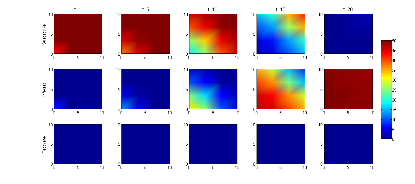
Figure 1. Dynamic of the system without control for $\alpha=1$.

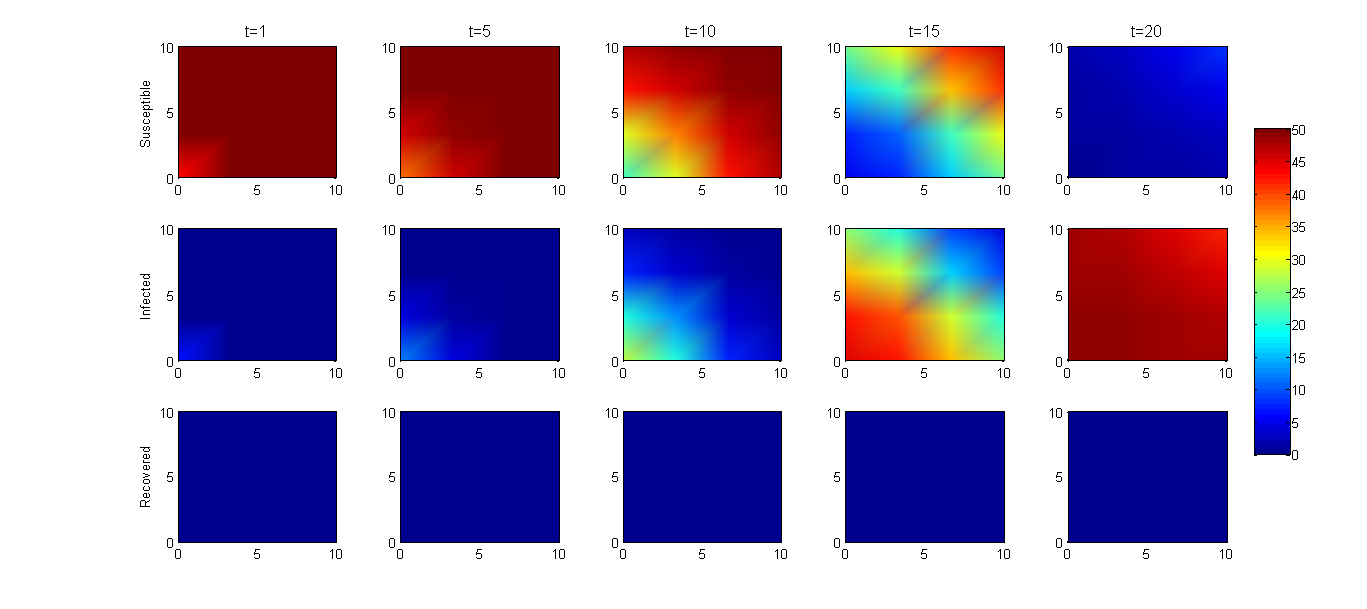
Figure 2. Dynamic of the system without control for $\alpha=0.95$.

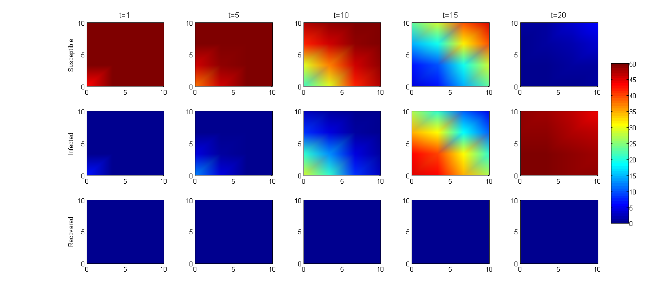
Figure 3. Dynamic of the system without control for $\alpha=0.9$.

7.2. Fractional $\alpha$-dynamics with optimal vaccination strategy

We compare the infection prevalence over a period of $20$ days in the presence of the vaccination strategy. We note that the susceptible individuals are transferred to the recovered class (see Figures 4, 5 and 6). In Figure 4, we see that the number of infected people is $40$ per cell and $10$ per cell for recovered individuals. In Figures 5 and 6, we have almost $5$ susceptible people per cell, $35$ infected people per cell, and $10$ recovered individuals per cell.

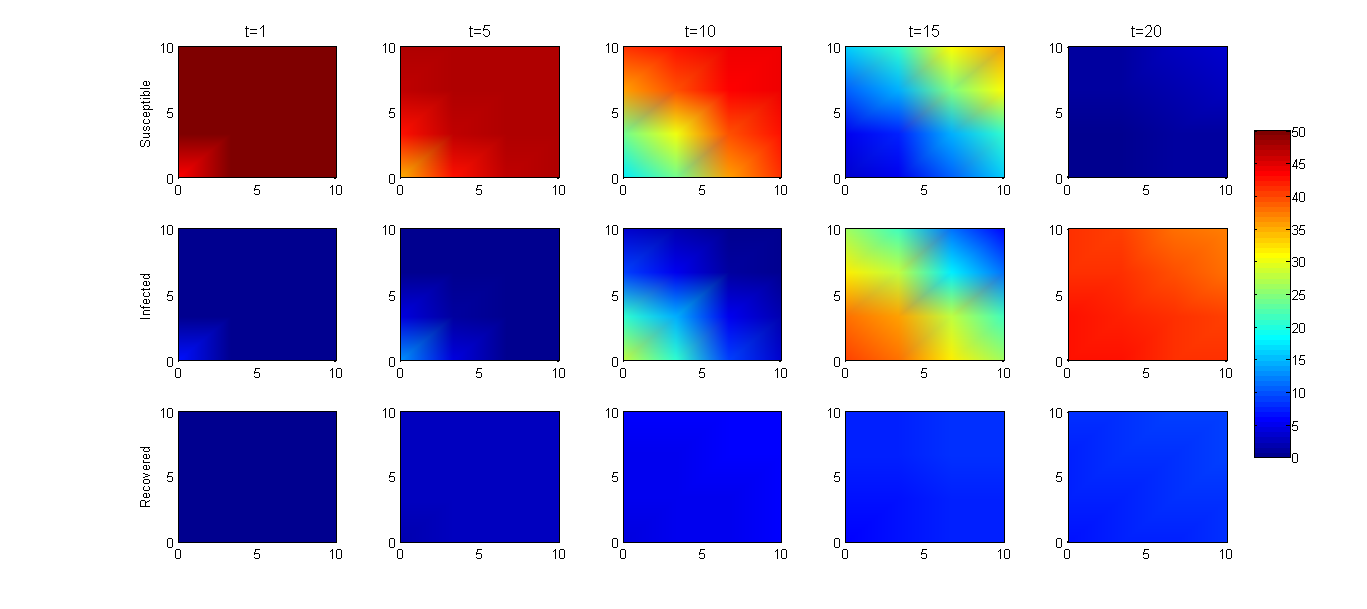
Figure 4. Dynamic of the system with control for $\alpha=1$.

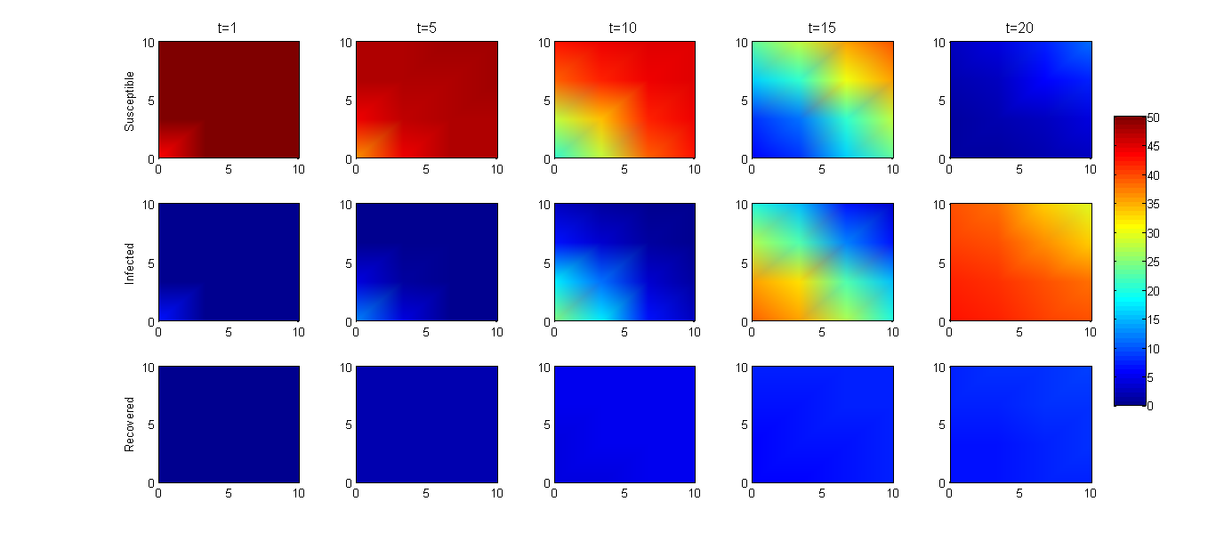
Figure 5. Dynamic of the system with control for $\alpha=0.95$.

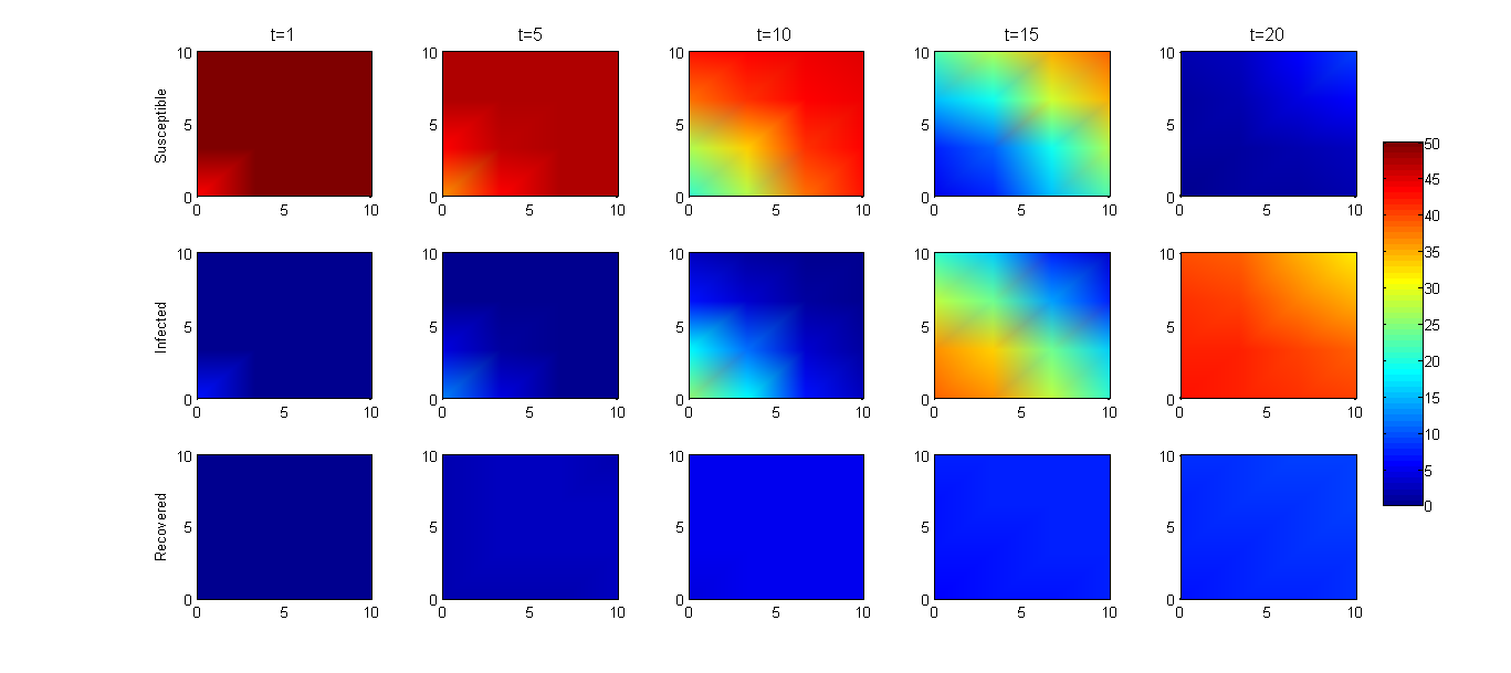
Figure 6. Dynamic of the system with control for $\alpha=0.9$.

Next, we investigate the effect of the order $\alpha$ to the value of the cost functional $J$ in absence and presence of vaccination. Before that, we present the results in Table  2 and Table  3, respectively.

Table 2. Values of the cost functional $J$ without control for different $\alpha$.

$\alpha$	0.9	0.95	1
J	$7.4350e^{+04}$	$7.1586e^{+04}$	$7.7019e^{+04}$

Table 3. Values of the cost functional $J$ with control for different $\alpha$.

$\alpha$	0.9	0.95	1
J	$4.9157e^{+04}$	$4.7489e^{+04}$	$5.2503e^{+04}$

We note that the functional $J$ decreases under the effect of vaccination for different values of $\alpha$, and the value of $J$ is optimal as $\alpha=0.95$. Furthermore, the results obtained in fractional order cases show that the spread of the disease takes more than 20 days to cover the entire space with the same cost of the vaccination strategy in the case of integer derivatives.

8. Conclusion

In this study, we investigated the optimal vaccination strategy for a fractional SIR model. Interactions between susceptible, infected, and recovered are modeled by a system of partial differential equations with Atangana–Baleanu–Caputo fractional time derivative. We proved existence of solutions to our fractional parabolic state system as well as the existence of an optimal control. For a given objective functional $J$, an optimal control is characterized in terms of the corresponding state and adjoint variables. In order to control the infection, we have compared the dynamics of our system with different values of $\alpha$. We noticed that the values of $J$ decreases under the effect of vaccination for different values of $\alpha$. Moreover, with the presence of an optimal vaccination strategy, we found that the smallest value of the cost-functional $J$ is obtained when $\alpha=0.95$. Then, an analysis of the proposed fractional order strategy with a well chosen fractional order $\alpha$ shows that it is more cost-effective than the classical strategy. Finally, the results obtained when $\alpha$ takes a fractional value show that the spread of the disease takes more than $20$ days to cover the entire space with the same cost of the vaccination strategy in the case of integer-order derivatives.

References

- [1] (MR3646671) [10.22436/jnsa.010.03.20] T. Abdeljawad and D. Baleanu, Integration by parts and its applications of a new nonlocal fractional derivative with Mittag–Leffler nonsingular kernel, J. Nonlinear Sci. Appl., 10 (2017), 1098–1107.
- [2] (MR1930721) [10.1016/S0022-247X(02)00180-4] O. P. Agrawal, Formulation of Euler–Lagrange equations for fractional variational problems, J. Math. Anal. Appl., 272 (2002), 368–379.
- [3] (MR3719831) [10.2298/AADM170428002A] R. Almeida, What is the best fractional derivative to fit data?, Appl. Anal. Discrete Math., 11 (2017), 358–368.
- [4] (MR3511679) [10.22436/jnsa.009.06.17] R. T. Alqahtani, Atangana–Baleanu derivative with fractional order applied to the model of groundwater within an unconfined aquifer, J. Nonlinear Sci. Appl., 9, (2016), 3647–3654.
- [5] [10.2298/TSCI160111018A] A. Atangana and D. Baleanu, New fractional derivatives with nonlocal and non–singular kernel: theory and application to heat transfer model, Thermal Science, 20 (2016), 763–769.
- [6] [10.1140/epjp/i2018-12021-3] A. Atangana and J. F. Gómez–Aguilar, Decolonisation of fractional calculus rules: Breaking commutativity and associativity to capture more natural phenomena, Eur. Phys. J. Plus, 133 (2018), Art. 166, 22 pp.
- [7] (MR3764302) [10.1515/fca-2017-0076] G. M. Bahaa, Fractional optimal control problem for variable–order differential systems, Fract. Calc. Appl. Anal., 20 (2017), 1447–1470.
- [8] [10.1115/DETC2009-87008] R. K. Biswas and S. Sen, Numerical method for solving fractional optimal control problems, In Proceedings of the ASME 2009 International Design Engineering Technical Conferences and Computers and Information in Engineering Conference, San Diego, CA, USA, (2010), 1205–1208.
- [9] (MR2849617) [10.1177/1077546310373618] R. K. Biswas and S. Sen, Fractional optimal control problems: A pseudo-state-space approach, J. Vib. Control, 17 (2010), 1034–1041.
- [10] (MR2849617) [10.1177/1077546310373618] R. K. Biswas and S. Sen, Fractional optimal control problems with specified final time, J. Comput. Nonlinear Dyn., 6 (2011), 021009.
- [11] [10.1115/DETC2011-48045] R. K. Biswas and S. Sen, Fractional optimal control within Caputo’s derivative, In Proceedings of the ASME 2011 International Design Engineering Technical Conferences and Computers and Information in Engineering Conference, Washington, DC, USA, (2012), 353–360.
- [12] (MR3151796) [10.1016/j.jfranklin.2013.09.024] R. K. Biswas and S. Sen, Free final time fractional optimal control problems, J. Frankl. Inst., 351 (2014), 941–951.
- [13] (MR3030124) [10.1007/s11071-012-0475-2] K. Diethelm, A fractional calculus based model for the simulation of an outbreak of dengue fever, Nonlinear Dyn., 71 (2013), 613–619.
- [14] [10.1109/TCST.2011.2153203] Y. Ding, Z. Wang and H. Ye, Optimal control of a fractional-order HIV-immune system with memory, IEEE Trans. Control Syst. Technol., 20 (2011), 763–769.
- [15] (MR3968302) [10.1007/s10957-018-1305-6] J. D. Djida, G. M. Mophou and I. Area, Optimal control of diffusion equation with fractional time derivative with nonlocal and nonsingular Mittag-Leffler kernel, J. Optim. Theory Appl. 182 (2019), 540–557.
- [16] (MR3019305) [10.1007/s10957-012-0233-0] T. L. Guo, The necessary conditions of fractional optimal control in the sense of Caputo, J. Optim. Theory Appl., 156 (2013), 115–126.
- [17] (MR3985793) [10.1007/s40435-019-00525-w] A. A. Laaroussi, R. Ghazzali, M. Rachik and S. Benrhila, Modeling the spatiotemporal transmission of Ebola disease and optimal control: a regional approach, Int. J. Dyn. Control, 7 (2019), no. 3, 1110–1124.
- [18] (MR2316829) S. Lenhart and J. T. Workman, Optimal Control Applied to Biological Models, Chapman and Hall, CRC Press, 2007.
- [19] (MR0259693) J-L. Lions Quelques méthodes de résolution des problèmes aux limites non linéaires, Dunod, Gauthier-Villars, Paris 1969.
- [20] (MR2739436) [10.1016/j.camwa.2010.10.030] G. M. Mophou, Optimal control of fractional diffusion equation, Comput. Math. Appl. 61 (2011), 68–78.
- [21] (MR2824729) [10.1016/j.camwa.2011.04.044] G. M. Mophou and G. M. N’Guérékata, Optimal control of fractional diffusion equation with state constraints, Comput. Math. Appl. 62 (2011), 1413–1426.
- [22] E. Okyere, F. T. Oduro, S. K. Amponsah and I. K. Dontwi, Fractional order optimal control model for malaria infection, arXiv preprint https://arxiv.org/abs/1607.01612, (2016).
- [23] (MR1658022) I. Podlubny, Fractional Differential Equations, Mathematics in Science and Engineering, 198, Academic Press, Inc., San Diego, CA, 1999.
- [24] (MR3872489) [10.1016/j.chaos.2018.10.021] S. Rosa and D. F. M. Torres, Optimal control of a fractional order epidemic model with application to human respiratory syncytial virus infectio, Chaos Solitons Fractals 117 (2018), 142–149. \arXiv1810.06900
- [25] (MR4232864) [10.1007/s11786-020-00467-z] M. R. Sidi Ammi, M. Tahiri and D. F. M. Torres, Global stability of a Caputo fractional SIRS model with general incidence rate, Math. Comput. Sci. 15 (2021), no. 1, 91–105. \arXiv2002.02560
- [26] (MR3988048) [10.1016/j.camwa.2019.03.043] M. R. Sidi Ammi and D. F. M. Torres, Optimal control of a nonlocal thermistor problem with ABC fractional time derivatives, Comput. Math. Appl. 78 (2019), no. 5, 1507–1516. \arXiv1903.07961
- [27] (MR3101449) [10.1016/j.mbs.2013.05.005] C. J. Silva and D. F. M. Torres, Optimal control for a tuberculosis model with reinfection and post-exposure interventions, Math. Biosci. 244, (2013), no. 2, 154–164. \arXiv1305.2145
- [28] (MR3395619) [10.1186/s13662-015-0593-5] Q. Tang and QX. Ma, Variational formulation and optimal control of fractional diffusion equations with Caputo derivatives, Adv. Diff. Equa. 2015 (2015), Art. 283, 14 pp.
- [29] (MR3876254) [10.1016/j.chaos.2018.11.009] S. Yadav, R.K. Pandey and A.K. Shukla, Numerical approximations of Atangana–Baleanu Caputo derivative and its application, Chaos, Solitons and Fractals, 118, (2019), 58–64.
- [30] [10.1109/CCDC.2015.7162031] J. Yuan, B. Shi, D. Zhang and S. Cui, A formulation for fractional optimal control problems via Left and Right Caputo derivatives, The 27th Chinese Control and Decision Conference (2015 CCDC), (2015), 816–821.