Microbiome compositional analysis with logistic-tree normal models

Abstract

Modern microbiome compositional data are often high-dimensional and exhibit complex dependency among the microbial taxa. However, existing statistical models for such data either do not adequately account for the dependency among the microbial taxa or lack computational scalability with respect to the number of taxa. This presents challenges in important applications such as association analysis between microbiome compositions and disease risk in which valid statistical analysis requires appropriately incorporating the “variance components” or “random effects” in the microbiome composition. We introduce a generative model, called the “logistic-tree normal” (LTN) model, that addresses this need. LTN marries two popular classes of models—namely, log-ratio normal (LN) and Dirichlet-tree (DT)—and inherits the key benefits of each. LN models are flexible in characterizing covariance structure among taxa but lacks scalability with respect to the number of taxa; DT is computationally more tractable through a tree-based binomial decomposition of the composition but at the same time it incurs restrictive covariance among the taxa. LTN incorporates the tree-based decomposition as the DT does, but it jointly models the corresponding binomial probabilities using a (multivariate) logistic-normal distribution as in LN models. It therefore allows rich covariance structures as LN, along with computational efficiency realized through a Pólya-Gamma augmentation on the binomial models associated with the tree splits. Accordingly, Bayesian inference on LTN can readily proceed by Gibbs sampling. LTN also allows common techniques for effective inference on high-dimensional data—such as those based on sparsity and low-rank assumptions in the covariance structure—to be readily incorporated. We construct a general mixed-effects model using LTN to characterize compositional random effects, which allows flexible taxa covariance. We demonstrate its use in testing association between microbiome composition and disease risk as well as in estimating the covariance among taxa. We carry out an extensive case study using this LTN-enriched compositional mixed-effects model to analyze a longitudinal dataset from the T1D cohort of the DIABIMMUNE project.

1 Introduction

The human microbiome is the collection of genetic information from all microbes residing on or within the human body. The development of high-throughput sequencing technologies has enabled profiling the microbiome in a cost-efficient way through either shotgun metagenomic sequencing or amplicon sequencing on target genes (e.g., the 16S rRNA gene). Various bioinformatic preprocessing pipelines such as MetaPhLAN (Beghini et al., 2021) and DADA2 (Callahan et al., 2016) have been developed to “count” the microbes in each sample and report the results in terms of amplicon sequence variant (ASV) or operational taxonomic unit (OTU) abundance. The resulting datasets are compositional in nature as the total counts of the identified microbes in each sample are determined by the sequencing depth of the study and shall only be interpreted proportionally. Both OTU and ASV can serve as the unit for the downstream analysis of microbial compositions, so for simplicity, we shall use the more classic term “OTU” to refer to either of them. Along with the OTU counts, a typical microbiome dataset also contains a summary of the evolutionary relationship of OTUs in the study in the form of a phylogenetic tree, and covariate information on the participant hosts that are usually collected by medical monitoring or questionnaires.

A central task in microbiome studies is to understand the relationship between microbiome compositions and environmental factors such as the dietary habits or the disease status of the hosts. Since individual microbiome samples are noisy and are prone to be polluted by sequencing errors, a popular practice toward this goal is to compare microbiome compositions across groups of samples defined by the factor of interest. For example, a core research question in the DIABIMMUNE study (Kostic et al., 2015) is to understand the association between infant gut microbiome and Type 1 diabetes (T1D) risk. To this end, previous studies compared microbiome compositions of case samples with healthy controls and have suggested that the gut microbiome of those T1D cases have significantly lower alpha diversity compared to the controls (Kostic et al., 2015).

Traditionally, such cross-group comparisons are achieved through either lower-dimensional summaries of the composition such as alpha diversity or distance-based methods like PERMANOVA (McArdle and Anderson, 2001). Alternatively, a more recent thread of works aims at comparing whole compositions to better account for the variety of possibly variations (Grantham et al., 2017; Tang et al., 2018; Mao et al., 2020; Ren et al., 2020). One fruitful strategy is through building generative models on microbiome compositions that account for key features of of such data including compositionality, high dimensionality, and complex covariance among taxa, which together pose analytical and computational challenges.

A common approach to accounting for the compositional and count nature of microbiome sequencing data is to adopt a multinomial sampling model for the sequencing read counts. Under this strategy, two popular classes of statistical models for the corresponding multinomial probability vector (i.e., the relative abundances of the OTUs) are log-ratio normal (LN) models (Aitchison, 1982) and the more recent Dirichlet-tree multinomial (DTM) model (Dennis III, 1991). The LN model can capture rich covariance structure among the OTUs; however, inference under such models, especially when they are embedded as a component into more sophisticated models, is computationally challenging when the number of OTUs is large ($>50$) due to lack of conjugacy to the multinomial likelihood.

The Dirichlet-multinomial (DM) model is another popular model for low-dimensional compositional data. It simply adopts a Dirichlet “prior”, conjugate to the multinomial sampling model, to account for cross-sample variability, but its induced covariance structure is characterized by a single scalar parameter, and thus is way too restrictive for microbiome abundances. The DTM is a generalization of the DM model, designed to lessen this limitation, while trying to maintain computational simplicity. The DTM preserves the conjugacy by decomposing the multinomial likelihood into a collection of binomials along the phylogenetic tree and modeling the binomial probabilities by beta distributions. With such a decomposition, DTM is conjugate and thus computationally efficient, but the covariance structure, though more relaxed than that of the Dirichlet, is still quite restrictive as it still only uses $K$ parameters to characterize a $K\times K$ covariance structure. Moreover, due to this constraint, the appropriateness of the covariance structure imposed by the DTM relies heavily on the similarity between the phylogenetic tree and the functional relationship among the taxa in the given context, making the resulting inference particularly sensitive to the specification of the tree.

It is also worth noting that while traditional wisdom suggests that the DTM (which contains DM as a special case) is computationally scalable due to the Dirichlet-multinomial conjugacy, applications of the DTM can incur prohibitive computation when it is not the only or top layer in a hierarchical model. That is, when the mean and dispersion parameters that specified a DTM are also unknown and modeled. This is because there exists no known conjugate (hyper)prior to Dirichlet, and hence to the DTM model. For example, when covariate effects on the mean of a DTM or when hyperpriors on the dispersion are incorporated, it will require numerical integration or MCMC strategies such as Metropolis-Hastings to infer these parameters. (If one is willing to sacrifice the Bayesian paradigm, it is also possible to adopt frequentist optimization strategies to compute point estimates or approximations to the parameters of DTM. In this work we consider a fully Bayesian strategy for inference.) Such numerical integration can still be extremely expensive as it will require a minimal of a 2D integral evaluated on each tree node in each MCMC iteration. As such, it is desirable to design a model that enjoys full conjugacy, or in other words has a conjugate (hyper)prior to itself.

We propose a new generative model called “logistic-tree normal” (LTN) that combines the key features of DTM and LN models to inherit their respective desired properties, and resolves the nonconjugacy issue completely. LTN utilizes the tree-based decomposition of multinomial model as DTM does but jointly model the binomial probabilities using a multivariate LN distribution with a general covariance structure. The more flexible covariance structure makes the resulting inference substantially more robust with respect to the choice of the partition tree than DTM, which is a common concern in microbiome analysis based on the phylogenetic tree (Xiao et al., 2018; Zhou et al., 2021). At the same time, by utilizing the tree-based binomial decomposition of the multinomial, LTN restores the full conjugacy with the assistance of Pólya-Gamma (PG) data augmentation (Polson et al., 2013), allowing Gibbs sampling for inference and thereby avoiding the computational difficulty incurred by the classic LN models.

The fully probabilistic, generative nature of the LTN model allows it to be used either as a standalone model or embedded into more sophisticated hierarchical models. With the PG augmentation, LTN has conjugate (hyper)priors and thus maintains full conjugacy even in the presence of additional hierarchical modeling on the mean and covariance, and thus avoids expensive numerical integration as required by DTM. Moreover, the multivariate Gaussian aspect of the model allows common assumptions for effective inference on high-dimensional data, such as those based on sparsity and low-rank assumptions in the covariance structure, to be readily incorporated while maintaining the computational ease.

The rest of the paper is organized as follows. Section 2 introduces the LTN model and describes mixed-effects modeling based on LTN. In Section 3, we investigate the performance of the proposed method with several numerical experiments and a real data application. Section 4 concludes.

2 Methods

2.1 Logistic-tree normal model for OTU counts

In this section we will briefly review the LN and the DTM models for microbiome compositional data, and then introduce the new logistic-tree normal (LTN) model.

Suppose there are $n$ samples and a total of $K$ OTUs, denoted by $u_{1},u_{2},\ldots,u_{K}$. The OTU table is an $n\times K$ matrix, whose $i$th row represents the OTU counts in sample $i$ and the $(i,j)$-th element represents the count of OTU $j$ in that sample. Let $\mathcal{T}=\mathcal{T(I,U;E)}$ be a rooted full binary phylogenetic tree over the $K$ OTUs, where $\mathcal{I,U,E}$ denote the set of interior nodes, leaves, and edges respectively. Formally, we can represent each node $A$ in the phylogenetic tree by the set of its descendent OTUs. Specifically, for a leaf node $A\in\mathcal{U}$, which by definition contains only a single OTU $u$, we let $A=\{u\}$. Then the interior nodes can be defined iteratively from leaf to root. That is, for $A\in\mathcal{I}$ with two children nodes $A_{l}$ and $A_{r}$, we simply have $A=A_{l}\bigcup A_{r}$. Figure 1(a) shows an example of a node $A$ containing four OTUs, $\{u_{1},u_{2},u_{3},u_{4}\}$.

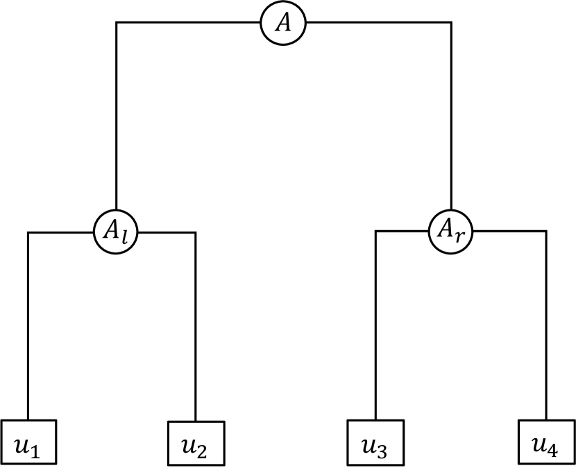
(a) Notation for nodes

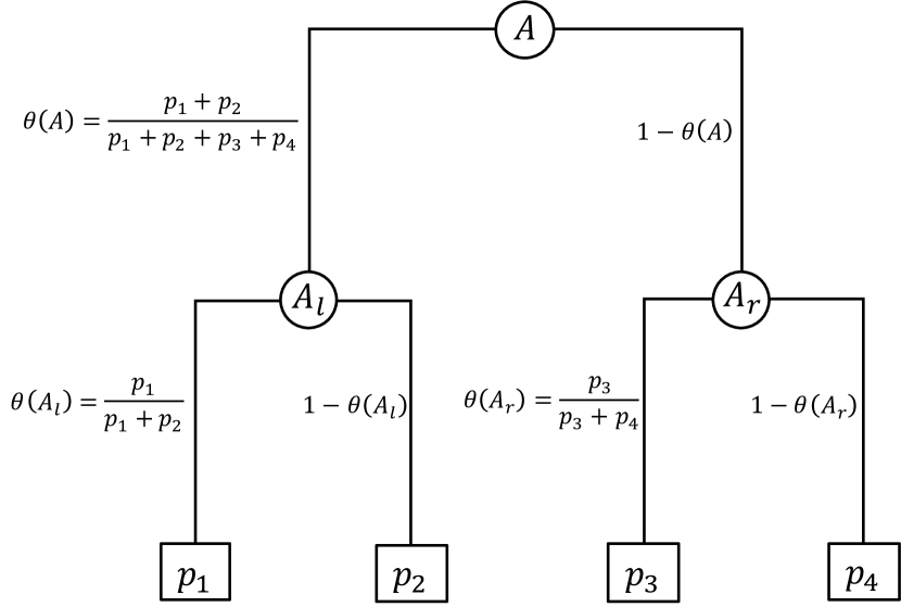
(b) Tree-based transform from $\boldsymbol{p}$ to $\boldsymbol{\theta}$

Figure 1: An example of a phylogenetic tree over four OTUs

Suppose $\boldsymbol{X}=(X_{1},\cdots,X_{K})^{\prime}$ is the OTU counts for a sample, and $N=\sum_{j=1}^{K}X_{j}$ is the total number of OTU counts. A natural sampling model for the OTU counts given the total count $N$ is the multinomial model

$$\boldsymbol{X}\,|\,N,\boldsymbol{p}\sim{\rm Multinomial}(N,\boldsymbol{p}),$$ (1)

where $\boldsymbol{p}=(p_{1},\cdots,p_{K})^{\prime}$ is the underlying OTU (relative) abundance vector, which lies in a $(K-1)$-simplex. That is, $\boldsymbol{p}\in\mathcal{S}_{K}=\{(p_{1},\cdots,p_{K})^{\prime}:p_{j}\geq 0,j=1,\cdots,K,\sum_{j=1}^{K}p_{j}=1\}$. The simplicial constraint on relative abundances can present modeling inconveniences, and a traditional strategy is to apply a so-called log-ratio transformation to map the relative abundance vector into a Euclidean space (Aitchison, 1982).

Three most popular choices of the log-ratio transform are the additive log-ratio (alr), centered log-ratio (clr) (Aitchison, 1982) and isometric log-ratio (ilr) (Egozcue et al., 2003; Egozcue and Pawlowsky-Glahn, 2016; Silverman et al., 2017), all of which have been applied to microbiome compositional data in the literature. For a composition $\boldsymbol{p}$, the alr and clr transforms are defined as follows:

$$clr(\boldsymbol{p})=\{\log(p_{j}/g(\boldsymbol{p})):j=1,\cdots,K\},$$

$$alr(\boldsymbol{p})=\{\log(p_{j}/p_{K}):j=1,\cdots,d\},$$

where $d=K-1$ and $g(\boldsymbol{p})$ is the geometric mean of $\boldsymbol{p}$. The ilr transform, on the other hand, uses a binary partition tree structure to define the log-ratios, and it turns $\boldsymbol{p}$ into “balances” associated with the interior nodes of the tree. The balance $\eta(A)$ associated with an interior node $A$ of the tree is defined as

$$\eta(A)=\sqrt{\frac{|A_{l}||A_{r}|}{|A_{l}|+|A_{r}|}}\log\frac{g(\boldsymbol{p}(A_{l}))}{g(\boldsymbol{p}(A_{r}))},$$

where $|A_{l}|$ and $|A_{r}|$ are the number of OTUs in the left and right subtree of node $A$ respectively, $g(\boldsymbol{p}(A_{l}))$ and $g(\boldsymbol{p}(A_{r}))$) are the corresponding geometric means of the probability compositions of leaves in the left and right subtrees of node $A$. While in many applications finding a suitable binary tree for the ilr might not be easy, in the microbiome context, the phylogenetic tree is a natural and effective choice (Silverman et al., 2017).

The log-ratio normal (LN) model posits that the log-ratios are multivariate Gaussian. These models have been successfully used in characterizing microbial dynamics (Äijö et al., 2017; Silverman et al., 2018) and linking covariates with microbiome compositions (Xia et al., 2013; Grantham et al., 2017). However, inference using the LN models based on the popular log-ratio transforms can incur prohibitive computational challenges when the number of OTUs grow due to the lack of conjugacy between the multinomial likelihood and multivariate normal.

In contrast, another classical approach to modeling the compositional vector $\boldsymbol{p}$ that is computationally easier at a (great) cost of flexibility is the Dirichlet model (La Rosa et al., 2012). This model affords only a single scalar parameter to characterize the covariance structure among the OTUs, essentially assuming that all OTUs are mutually independent modulo the artificial dependence caused by the compositional constraint $\sum_{j}p_{j}=1$. This is clearly too restrictive for high-dimensional compositional data such as microbiome compositions.

The Dirichlet-tree multinomial model (DTM) (Dennis III, 1991) has been introduced to alleviate this limitation of the Dirichlet while maintaining computational tractability. Given a dyadic tree $\mathcal{T}$ over the OTUs, e.g., the phylogenetic tree, the DTM utilizes the fact that multinomial sampling is equivalent to sequential binomial sampling down a binary partition. Specifically, the multinomial sampling model in Eq. (1) is equivalent to

$$y(A_{l})\,|\,y(A),\theta(A)\stackrel{{\scriptstyle\rm ind}}{{\sim}}{\rm Binomial}(y(A),\theta(A))\qquad\text{for all }A\in\mathcal{I},$$

where

$$y(A)=\sum_{j:u_{j}\in A}X_{j}\qquad\text{and}\qquad\theta(A)=\frac{\sum_{j:u_{j}\in A_{l}}p_{j}}{\sum_{j:u_{j}\in A}p_{j}}.$$

See Figure 1(b) for an illustration.

Under this perspective, the relative abundance vector is now represented using the collection of binomial “branching” probabilities $\theta(A)$ for all $A\in\mathcal{I}$. The DTM adopts a beta model for each $\theta(A)$ to attain conjugacy with respect to the binomial likelihood. That is,

$$\theta(A)\stackrel{{\scriptstyle\rm ind}}{{\sim}}{\rm Beta}(\mu(A)\nu(A),(1-\mu(A))\nu(A))\qquad\text{for }A\in\mathcal{I},$$

where $\mu(A)$ specifies the mean of the branching probabilities, and the variance is determined by $\mu(A)$ and $\nu(A)$. While it may appear similar to the ilr-based LN approach, which also uses the phylogenetic tree in transforming the abundance vector, we note that very importantly the factorization under the DTM is not only providing a transform of $\boldsymbol{p}$ in terms of the $\theta(A)$’s, but is decomposing the sampling model (i.e., the multinomial likelihood), which is key to its computational tractability through the beta-binomial conjugacy.

While DTM is more flexible than Dirichlet, it is far from competitive to LN in characterizing the covariance among OTUs. To see this, note that the parameters $\nu(A)$’s are the only ones that characterize the covariance across the $K$ OTUs. In fact, DTM still assumes independence among the $\theta(A)$’s and so there are a total of only $d$ scalar parameters, which along with the underlying phylogenetic tree characterize the covariance among the $K$ OTUs. This also makes inference with DTM particularly sensitive to the phylogenetic tree in each given application. In contrast, LN models, including the tree-based ilr models, allow a full $d\times d$ covariance matrix, regardless of the tree structure, which results in more robust inference even when the choice of the partition tree is not ideal. Also, as mentioned earlier since there is no known (hyper)prior for Dirichlet, DTM will still incur computational challenges should there be additional modeling hierarchies involved, such as covariate effects on its mean and priors on the unknown dispersion parameters, as those features will also break the conjugacy resulting in the need for numerical integration.

Motivated by LN and DTM, we introduce a hybrid model that combines the tree-based factorization of the multinomial sampling model under DTM with the log-ratio transform under LN, thereby achieving both the flexibility and the computational tractability. Specifically, we adopt a log-ratio transform (i.e., a logistic transform) on the binomial branching probability $\theta(A)$ on each interior node $A$. That is, we propose to model the log-odds on the interior nodes

$$\psi(A)=\log\frac{\theta(A)}{1-\theta(A)}\qquad\text{for all }A\in\mathcal{I}$$

jointly as a multivariate Gaussian.

More formally, for a compositional probability vector $\boldsymbol{p}=(p_{1},p_{2},\ldots,p_{K})\in\mathcal{S}_{K}$, we define the tree-based log-ratio (tlr) transform as $tlr(\boldsymbol{p})=\boldsymbol{\psi}=\{\psi(A):A\in\mathcal{I}\}$, where $\psi(A)=\log\frac{\theta(A)}{1-\theta(A)}$. Like other log-ratio transforms, $tlr$ maps a compositional vector $\boldsymbol{p}$ to a vector of $d$ log-odds $\psi(A)$. Finally, modeling the $tlr(\boldsymbol{p})$ as MVN$(\boldsymbol{\mu},\boldsymbol{\Sigma})$, we have the full formulation of a logistic-tree normal (LTN) model:

$$\begin{split}y(A_{l})|y(A),\theta(A)&\stackrel{{\scriptstyle\rm ind}}{{\sim}}{\rm Binomial}(y(A),\theta(A))\qquad\text{for }A\in\mathcal{I},\\ \ \psi(A)&=\log\frac{\theta(A)}{1-\theta(A)}\qquad\text{for }A\in\mathcal{I},\\ \boldsymbol{\psi}&\sim{\rm MVN}(\boldsymbol{\mu},\boldsymbol{\Sigma}).\end{split}$$ (2)

We denote this model by LTN${}_{\mathcal{T}}(\boldsymbol{\mu},\boldsymbol{\Sigma})$. A graphical model representation of the LTN model for a dataset with $n$ exchangeable samples indexed by $i=1,\cdots,n$ is shown in Figure 2(a).

At first glance, while LTN affords flexible mean and covariance structures, it suffers from the same lack of conjugacy as existing LN models based on log-ratio transforms such as alr, clr and ilr. Fortunately, the binomial decomposition of the likelihood under LTN allows a data-augmentation technique called Pólya-Gamma (PG) augmentation (Polson et al., 2013) to restore the conjugacy. In fact, this data-augmentation strategy ensures full conjugacy for LTN models even with additional modeling hierarchical such as covariates and multiple variance components, as one can adopt a variety of conjugate (hyper)priors on the Gaussian parameters $(\boldsymbol{\mu},\boldsymbol{\Sigma})$, making LTN substantially more computationally tractable than DTM.

A graphical model representation of LTN with PG augmentation for a dataset of $n$ exchangeable samples is shown in Figure 2(b). Details of the Pólya-Gamma augmentation for LTN are provided in Supplementary Material A.1.

(a) original model

(b) with Pólya-Gamma augmentation:
$w_{i}(A)|y_{i}(A),\psi_{i}(A)\stackrel{{\scriptstyle\rm ind}}{{\sim}}PG(y_{i}(A),\psi_{i}(A))$ is introduced to restore conjugacy

Figure 2: A graphical model representation of LTN for $n$ exchangeable samples

2.2 Mixed-effects modeling

Next we demonstrate the applicability of LTN through building a mixed-effects model on the compositional counts for longitudinal studies. Mixed-effects models are arguably the most useful statistical device for incorporating study designs into modeling microbiome compositions. Common design features such as covariates, batch effects, multiple time points, and replicates can all be readily incorporated.

For demonstration, consider a common study design where a dataset involves $n$ samples that can be categorized into two contrasting groups (e.g., case vs control, treatment vs placebo, etc.), and the practitioner is interested in testing whether there is cross-group difference in microbiome compositions. For each microbiome composition sample $i$, let $s_{i}\in\{0,1\}$ be the group indicator and $\boldsymbol{z}_{i}$ a $q$-vector of covariates.

We consider random effects that involve measured subgrouping structure (e.g., individuals). Specifically, we assume that there is a random effect for each sample $i$ associated with an observed grouping $g_{i}\in\{1,\cdots,G\}$. For example, in longitudinal studies, $g_{i}$ can represent the individual from which the $i$th sample is collected. We associate the covariates and random effects with the microbiome composition through the following linear model:

$$\boldsymbol{\psi}_{i}=\boldsymbol{\alpha}s_{i}+\boldsymbol{\beta}^{T}\boldsymbol{z}_{i}+\boldsymbol{\gamma}_{g_{i}}+\boldsymbol{\epsilon}_{i},$$ (3)

where $\boldsymbol{\alpha}$ represents the potential cross-group differences, $\boldsymbol{\beta}$ is a $q\times d$ matrix of unknown fixed effect coefficients of the covariates, $\boldsymbol{\gamma}_{g_{i}}$ is the random effect from individual $g_{i}$, which we model exchangeably as $\boldsymbol{\gamma}_{g}\stackrel{{\scriptstyle\rm iid}}{{\sim}}{\rm MVN}(\boldsymbol{0},\boldsymbol{\Sigma})$ for $g=1,\cdots,G$, and $\epsilon_{i}(A)\stackrel{{\scriptstyle\rm ind}}{{\sim}}{\rm N}(0,\sigma_{\epsilon}^{2}(A))$. We adopt inverse-Gamma prior on $\sigma_{\epsilon}^{2}(A)$.

Under this formulation, testing two-group difference can be accomplished through testing a collection of hypotheses on the interior nodes:

$$H_{0}:\alpha(A)=0\text{ versus }H_{1}:\alpha(A)\neq 0\qquad\text{for }A\in\mathcal{I}$$

To perform these local tests, we adopt a Bayesian variable selection strategy and place the following spike-and-slab priors on entries of $\boldsymbol{\alpha}$:

$$\alpha(A)|\pi(A),\phi_{\alpha} \stackrel{{\scriptstyle\rm ind}}{{\sim}}(1-\pi(A))\delta_{0}+\pi(A)(1-\delta_{0}){\rm N}(0,1/\phi_{\alpha})\qquad\text{for }A\in\mathcal{I},$$

$$\pi(A) \stackrel{{\scriptstyle\rm iid}}{{\sim}}{\rm Beta}(m,1-m)\qquad\text{for }A\in\mathcal{I},$$

$$\phi_{\alpha} \sim{\rm Gamma}(t,u),$$

where $\delta_{0}$ is point mass at 0, and $m,t,u$ are pre-specified hyperparameters. We adopt continuous priors on the coefficients of the covariates: $\boldsymbol{\beta}\sim{\rm N}_{q\times d}(0,cn\boldsymbol{I}_{d}\otimes(\boldsymbol{Z}^{T}\boldsymbol{Z})^{-1})$.

Existing literature on microbiome mixed-effects modeling have adopted the low-rank assumption on the covariance structure through introducing latent factors (Grantham et al., 2017; Ren et al., 2020). The LTN framework allows both low-rankness and sparsity to be readily incorporated using existing techniques in multivariate analysis. For demonstration and to investigate the usefulness of sparsity in this context, in the following example we impose sparsity by adopting a graphical Lasso prior on the inverse covariance of random effects. Specifically, the Bayesian graphical lasso prior (Wang, 2012) on $\boldsymbol{\Omega}=\boldsymbol{\Sigma}^{-1}$ takes the form

$$p(\boldsymbol{\Omega}|\lambda)=C^{-1}\prod_{j<j^{\prime}}\{{\rm DE}(\omega_{jj^{\prime}}|\lambda)\}\prod_{j=1}^{d}\{{\rm EXP}(\omega_{jj}|\lambda/2)\}{1}_{\boldsymbol{\Omega}\in M^{+}},$$

where DE$(x|\lambda)=\frac{\lambda}{2}{\exp}(-\lambda|x|)$ is the double exponential density function, EXP$(x|\lambda)=\lambda\exp(-\lambda x)1_{x>0}$ is the exponential density function, $M^{+}$ is the space of positive definite matrices, and $C$ is the normalizing constant that does not involve $\boldsymbol{\Omega}$ or $\lambda$.

Posterior sampling on this model can be conducted using a blocked Gibbs sampling scheme proposed in Wang (2012). With the Pólya-Gamma augmentation, all parts of the model can be drawn from conjugate full conditionals. The details of the sampler are included in Supplementary Materials A.3.

Based on the posterior samples, we can compute Pr$(\alpha(A)\neq 0|\boldsymbol{Y})$, the posterior marginal alternative probability (PMAP) for each $A\in\mathcal{I}$, and Pr$(\boldsymbol{\alpha}\neq\boldsymbol{0}\,|\,\boldsymbol{Y})$, the posterior joint alternative probability (PJAP). The PJAP can be used as a test statistics for rejecting the null hypothesis that no difference at all exists in any microbial taxa between the two groups, whereas PMAP can be used to investigate what microbial taxa are actually different across groups should PJAP indicates that such a difference exists. Both the PMAPs and PJAP can be directly estimated from the posterior samples of $\boldsymbol{\alpha}$.

We note that LTN could also be applied as a standalone generative model for learning the covariance structure among taxa by a sparse Gaussian graph. Indeed, this can be viewed as a special case of the mixed-effects model where $q=1,s_{i}=0,\epsilon_{i}=0,z_{i}=1,g_{i}=i$ for $i=1,\cdots,n$, and the covariance among the nodes is characterized by $\boldsymbol{\Omega}$. Other types of covariance structure of interest (e.g. $clr$ covariance matrix), can be easily obtained via Monte Carlo based on this generative model. We provide more details on posterior inference of the covariance structure in supplementary material A.2.

3 Results

3.1 Simulation studies

In this section, we carry out simulation studies to demonstrate the work of LTN in two-group comparison and covariance estimation based on a mixed-effects model as described in Section 2.2.

We first carry out simulation studies to evaluate the performance of the proposed LTN mixed-effects model in two-group comparison. We compare the proposed mixed-effects model in testing the null that there is no cross-group difference with a state-of-the-art mixed-effects model for microbiome compositions called DirFactor (Ren et al., 2020). DirFactor induces a marginal Dirichlet process prior for the OTU compositions and assumes a low-rank covariance structure in the random effects. Synthetic datasets are generated based on the real data analyzed in case study (Section 3.2). For the simulation, we use a subset of the data with $n=428$ samples, and we focus on the top 100 OTUs with highest relative abundance. The phylogenetic tree of these 100 OTUs is used throughout the simulations. In each simulation round, we randomly divide the samples into two equal-sized groups to generate data under the null, i.e., there is no cross-group difference. Two different scenarios of the alternative are considered: (1) Strong signal at a single OTU by increasing the count of one OTU by $200\%$ in one group, and (2) weak signal at multiple OTUs by increasing the counts of 8 OTUs by $50\%$ in one group.

We fit the mixed-effects model described in Section 2.2 as well as DirFactor to test the existence of differences in microbiome compositions across the two groups. Age at collection is included as a fixed effect, and individuals from which the samples were taken are treated as random effects. The ROC curves of these two approaches are shown in Figure 3. Under both scenarios, LTN has higher power than DirFactor at low to moderate false positive rates. Interestingly, the ROC curves of DirFactor under the two scenarios are similar, while performance of LTN is improved when cross-group differences occur at multiple OTUs. This might be because the signals at multiple OTUs, though relatively weak, could be aggregated along the tree and thus be identified with LTN at their common ancestors.

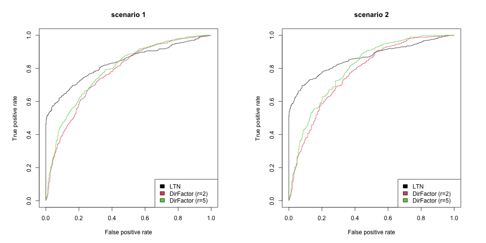
Figure 3: ROC curves under the two simulation scenarios. $r$ is the number of latent factors in DirFactor. The shrinkage parameter $\lambda$ of graphical lasso prior in LTN is set to 10. Left: Cross-group difference exists at a single OTU. In each simulation, we randomly select one of the top 20 OTUs with the highest relative abundance and increase the count of this OTU by $200\%$ in the second group. Right: Cross-group difference exists at multiple OTUs. In each simulation, we randomly select eight OTUs from the top 20 OTUs and increase the count of these OTUs by $50\%$ in the second group.

Next we assess the performance of LTN in terms of covariance estimation and use as a benchmark a state-of-the-art approach called COAT recently introduced in Cao et al. (2019). We simulate datasets with $n=200$ samples and $K=100$ OTUs with fixed phylogenetic tree. We purposefully generate data from LN and DTM to show that even under such model misspecification, the LTN can recover the true covariance structure in a robust manner. We set the parameters of DT to their method of moments estimates based on the same dataset used in two-group comparison simulation study to mimic real data. For LN, we consider three models – Hub, Block and Sparse for the precision matrix under (phylogenetic) $ilr$ transform, which are considered by Cao et al. (2019) as plausible covariance models for microbiome compositions. Further details on the simulation setting can be found in the Supplementary Material B.1.

For the comparison with COAT, we consider four different loss functions—the Frobenious norm, $L_{1}$ norm, entry-wise $L_{\infty}$ norm and the spectral norm of the difference between the estimated clr correlation matrix and the truth. We examine these losses on the clr correlation matrix because COAT aims at estimating the clr covariance, and can only be applied for estimating the clr covariance, while the generative nature of our proposed model can evaluate the induced covariance under the clr transform—or any other transform for that matter—based on the inferred model.

Table 1: Comparisons of risks of two methods under different simulation settings

	LN-Hub			LN-Block			LN-Sparse			DTM
	LTN	COAT		LTN	COAT		LTN	COAT		LTN	COAT
Frobenius	41.46	46.64		40.21	43.33		38.64	52.95		20.81	19.55
$L_{1}$	54.98	76.23		53.11	73.21		56.98	78.80		32.34	33.42
$L_{\infty}$	1.42	1.72		1.47	1.69		1.54	1.74		0.74	0.75
spectral	38.96	34.67		36.86	31.84		35.37	41.22		19.00	19.08

The results are presented in Table 1. Under the LN-sparse setting, LTN outperforms COAT under all four losses. Under the other simulation settings, LTN outperforms COAT under most losses. The flexibility of the multivariate normal allows LTN to effectively characterize the cross-sample variability even when the distribution of the relative abundances is misspecified. As shown in Supplementary Material B.2, the results are robust to the choice of the hyperparameters $\lambda$ and $c$ within certain ranges.

To understand the extent to which the inference based on LTN is sensitive to adoption of the phylogenetic tree, we carried out a sensitivity analysis based on simulation studies and present the results in Supplementary Material C. In summary, we compared the estimates of mean and covariance of the log-odds with LTN based on the correct and misspecified trees. The choice of the tree structure could potentially affect the inference from two aspects. First, it results in different parametrization of multinomial mean, and thus in particular may lead to less effective (i.e., parsimonious) representation of the underlying mean and covariance structure. This generally demonstrates itself in terms of larger posterior uncertainty. Secondly, misspecified trees could also introduce bias into this inference as it might place unreasonable constraint on the underlying mean and covariance. This concern should be much lessened under LTN compared to, say, DTM, as LTN still allows all possible covariance structure even when the tree structure is misspecified. Indeed, the sensitivity analysis reported in Supplementary Material C confirms that the inference of the mean and covariance structure based on LTN with misspecified trees is generally robust even when the tree is grossly incorrect. However, sensitivity does arise at very deep taxonomic levels given the limited amounts of data.

3.2 Case study: DIABIMMUNE data

In this section, we apply the mixed-effects model described in Section 2.2 to the Type 1 diabetes (T1D) cohort of DIABIMMUNE project to study the relationship of microbiome composition with certain covariates. This study collects longitudinal microbiome samples from 33 infants from Finland and Estonia. The full dataset contains counts of 2240 OTUs from 777 samples. The main goal of this study is to compare microbiome in infants who have developed T1D or serum autoantibodies (markers predicting the onset of T1D) with healthy controls in the same area. Within the time-frame of the study, 11 out of 33 infants seroconverted to serum autoantibody positivity, and of those 11 infants, four developed T1D. Previous studies on this dataset have established associations between the microbiome composition with both the T1D status as well as environmental and diet factors. For example, it has been shown that the microbiome of T1D patients tends to have a reduced diversity and increased prevalence of Bacteriodetes taxa (Dedrick et al., 2020; Kostic et al., 2015; Brugman et al., 2006). We focus on T1D status and dietary covariates and study the relationship between microbiome composition with each of the factors. Specifically, our analysis takes three steps for each single factor: (1) dichotomize the samples into two groups based on the level or value of the factor; (2) compare the microbiome compositions at the group level; and (3) identify and report the taxa that show such differences.

Key scientific findings from our analysis are summarized as follows: (i) the microbiome compositions of samples collected from T1D cases and seroconverters are not significantly different from the healthy controls; (ii) the microbiome compositions of samples taken after seroconversion differ from the other samples in terms of the relative abundance within two genera: Bacteroides and Parabacteroides, which are different from the taxa associated with T1D identified in Kostic et al. (2015); (iii) introduction of several kinds of food and cessation of breastfeeding can significantly alter the gut microbiome of the infants. We present details of our study on different host-level factors in the following sections.

3.2.1 T1D status

The DIABIMMUNE dataset records the T1D status of the individuals at the end of the study as one of the three levels: control, seroconverted and T1D onset. This status is used to define the case and control groups, where the case group consists of both seroconverted individuals and those who are clinically classified as T1D. For those in the case group, the age at seroconversion is also recorded.

We perform two comparisons regarding the T1D status variable: (1) a classic case versus control comparison is provided to retrospectively determine the association between gut microbiome and T1D, where $s_{i}=1$ for the cases, and (2) a comparison between the samples collected after seroconversion and the others to detect potential changes in microbiome compositions after seroconversion, where we set $s_{i}=1$ for samples collected after seroconversion.

In each comparison, we include a set of environmental and diet factors that might be associated with the microbiome composition as fixed effects to control false positives. First, we include eight binary dietary variables that indicate whether a specific type of diet was consumed at the time when the sample was collected: breastfeeding, solid food, eggs, fish, soy products, rye, barley, and buckwheat and millet. Age at collection (log-transformed), gender and nationality of the individuals are also included as fixed effects. In addition, individual random effects are included to account for the between-individual variation. We note that adjusting for these covariates are crucial for identifying the real cross-group differences (see Supplementary Material D.1).

We focus on the top 100 OTUs with highest relative abundance and take $\lambda=10$. The PJAPs of the case/control and pre-/post-seroconversion comparisons are 0.56 and 1.00, respectively. This indicates that overall there is no sufficient evidence that the microbiome composition distinguishes the cases and controls; instead, there are significant changes in the relative abundance of certain taxa, which—though might not be direct consequences of seroconversion—occur around the time of seroconversion. We provide visualization of the PMAPs on the phylogenetic tree in Figure 4. Three nodes, marked as $A_{1}$, $A_{2}$ and $A_{3}$, stand out, where descendants of $A_{1}$ and $A_{2}$ all belong to the genus Bacteroides. This result resonates with previous findings of changes in relative abundance of Bacteroides species in T1D cases compared to healthy controls (Giongo et al., 2011; Davis-Richardson et al., 2014; Vatanen et al., 2016). The descendants of node $A_{3}$ are Parabacteroides, and the left child of $A_{3}$ is distasonis. The posterior mean of $\alpha(A_{3})$ is positive. With small PMAPs at all ancestors of $A_{3}$, the positive $\hat{\alpha}(A_{3})$ indicates a higher relative abundance of the left subtree, the distasonis, in the post-seroconversion samples. The species distasonis has not been identified as associated with T1D or seroconversion in the original study of this dataset by Kostic et al. (2015); however, the large PMAP at $A_{3}$ is consistent with the data, where post-seroconversion samples show higher relative abundance of distasonis at older age (Figure 7(a)).

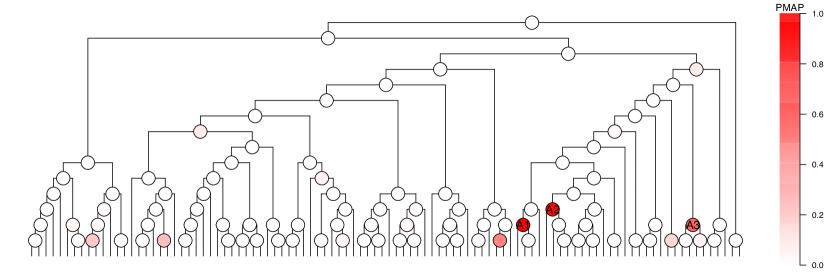
Figure 4: PMAPs of seroconversion. The nodes are colored by PMAP. Descendants of A1 and A2 all belong to the genus Bacteroides. The descendants of node A3 are Parabacteroides, and the left child of A3 is distasonis. The positive $\hat{\alpha}(A_{3})$ indicates a higher relative abundance of the left subtree, the distasonis, in the post-seroconverted samples.

3.2.2 Dietary factors

We also compare the microbiome composition of groups of samples differentiated by each of the eight dietary factors introduced in Section 3.2.1. In particular, the cessation of breastfeeding and the introduction of other types of food are registered continuously. Thus we are essentially comparing the microbiome compositions in samples taken before and after those change points of diet. Similar to Section 3.2.1, we include the T1D status, other dietary covariates, and environmental covariates including age, gender and nationality as fixed effects, individuals as random effects in our mixed effects model. The sample size under different comparisons as well as the PJAPs with $\lambda=10$ are shown in Table 2.

Table 2: PJAPs of the dietary variables

Variable	Group size		PJAP
	On ($s_{i}=1$)	Off ($s_{i}=0$)
Barley	531	246	1.00
Breastfeeding	248	529	1.00
Buckwheat&Millet	198	579	1.00
Eggs	477	300	0.75
Fish	581	196	1.00
Rye	514	263	0.83
Solid Food	681	96	1.00
Soy Product	107	670	1.00

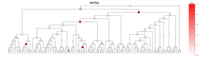
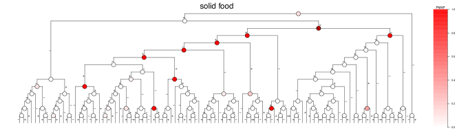
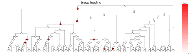
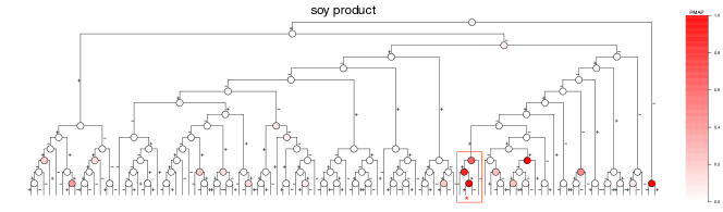
Figure S8: PMAPs of five dietary variables. For each node $A$, the sign of posterior mean of $\alpha(A)$ is marked with “+”/“-” on left and right branches. Node A0 has large PMAP in three comparisons and it corresponds to the “Firmicutes/Bacteroides ratio”. OTU 4439360 is marked with “*”, and its three ancestors form a chain of large PMAPs that indicates cross-group difference in relative abundance of OTU 4439360.

We visualize PMAPs of the dietary variables on the phylogenetic tree in Figure S8. Two interesting patterns are observed in the PMAPs. First, the node whose left and right child are Firmicutes and Bacteroidetes has high PMAP for three dietary variables: barley, rye and solid food. This implies that introduction of these three food is associated with changes in the “Firmicutes/Bacteroides ratio”, which is widely used as an index of dysbiosis (Stojanov et al., 2020). Second, chains of large PMAPs are observed in some comparisons, which can be useful in targeting the taxa contributing to the cross-group difference. For example, for soy product, a chain of three ancestors of OTU 4439360 with the same direction of changes in the relative abundance implies higher relative abundance of OTU 4439360 after introducing soy product, which is consistent with data at older age (see Figure 7(b)).

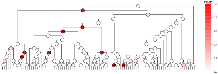
Figure S10: PMAPs of the comparison between samples collected before and after cessation of breastfeeding

In addition to these common patterns, we investigate how breastfeeding shapes the gut microbiome development. The inferred model suggest reduced Lachnospiraceae relative to Veillonellaceae and increased Bifidobacterium in samples collected from infants during breastfeeding; in particular, the enrichment of Bifidobacterium can be attributed to longum and bifidum as well as some other unclassified species. Such results are consistent with previous findings Kostic et al. (2015); Gueimonde et al. (2007); Fehr et al. (2020). PMAPs are visualized on the tree in supplementary Figure S10, and information of nodes with PMAP$>$0.5 are listed in supplementary Table S1.

4 Conclusions

We have introduced the LTN model as a general-purpose model for microbiome compositions. LTN decomposes the multinomial sampling model to a collection of binomials at the interior nodes of the phylogenetic tree, and transforms OTU compositions to node-specific log-odds and adopts multivariate normal model on the log-odds, hence possesses the benefits of both LN and DT models. In particular, the multivariate normal model on the log-odds offers flexible covariance structure among OTUs. With the tree-based decomposition, LTN avoids the computational challenges caused by the lack of conjugacy between multinomial and multivariate normal in LN models, and efficient inference can be carried out with Gibbs sampling by introducing Pólya-Gamma auxiliary variables. This opens the door to adopting a wide range of multivariate analysis models/methods for microbiome analysis while maintaining computational tractability.

The LTN model can be used either as a standalone model or a component in more sophisticated models such as those involving covariate effects and latent structures, which are often needed in microbiome applications. We have provided examples of mixed-effects modeling for cross-group comparison and for inference on the covariance structure to demonstrate its broad applicability. In the covariance estimation example, we have adopted the graphical Lasso prior on the inverse covariance matrix of the log-odds to infer an underlying sparse graph among the interior nodes of the phylogenetic tree. In mixed-effects modeling, we have shown how to carry out cross-group comparison of microbiome compositions through a Bayesian model choice framework. In these examples, our model/prior choices can be substituted with other existing approaches as the practitioner sees fit in the given context.

Finally, we note that while our domain context is microbiome analysis, the LTN model is more broadly applicable to other compositional data along with a binary tree partition over the compositional categories. In other contexts, such a tree can often be obtained based on domain knowledge or from data-driven approaches such as hierarchical clustering. Beyond compositional data, tree-based log-odds decompositions can also be used as device for modeling general probability distributions (Jara and Hanson, 2011), the modeling and inference strategies described herein can be applied in these broader contexts as well.

Software

We provide an R package (LTN: https://github.com/MaStatLab/LTN) implementing the proposed method. Source code for the numerical examples and case study is available at https://github.com/MaStatLab/LTN_analysis1.

Acknowledgements

LM’s research is supported by NIH grant R01-GM135440 as well as NSF grants DMS-1749789 and DMS-2013930.

Supplementary materials

A Inference strategy

A.1 Pólya Gamma augmentation for LTN

In this section we describe the Pólya Gamma augmentation scheme for the proposed LTN method. The binomial sampling model is

$$y(A_{l})|\psi(A),y(A))\stackrel{{\scriptstyle\rm ind}}{{\sim}}{\rm Binomial}\left(y(A),\frac{e^{\psi(A)}}{e^{\psi(A)}+1}\right)\qquad\text{ for all }A\in\mathcal{I}$$

Following Polson et al. (2013), we can write the binomial likelihood for a sample at an interior node $A$ as

$$p(y(A_{l})|y(A),\psi(A))\propto\frac{\left(e^{\psi(A)}\right)^{y(A_{l})}}{\left(1+e^{\psi(A)}\right)^{y(A)}} =2^{-y(A)}e^{\kappa(A)\psi(A)}\int_{0}^{\infty}e^{-w\psi(A)^{2}/2}f(w)dw,$$

where $\kappa(A)=y(A_{l})-y(A)/2$ and

$$f(w)=\frac{2^{y(A)-1}}{\Gamma(y(A))}\sum_{n=0}^{\infty}(-1)^{n}\frac{\Gamma(n+y(A))}{\Gamma(n+1)}\frac{(2n+y(A))}{\sqrt{2\pi w^{3}}}e^{-\frac{(2n+y(A))^{2}}{8w}}$$

is the probability density function of the Pólya-Gamma distribution PG$(y(A),0)$. We can accordingly introduce an auxiliary variable $w(A)$ that is independent of $y(A_{l})$ given $y(A)$ and $\psi(A)$, with

$$p(w(A)|y(A),\psi(A))\propto e^{-w(A)\psi(A)^{2}/2}f(w(A)).$$

In other words, we add the auxiliary variable $w(A)$ into the LTN model in Eq. (2) with

$$w(A)|y(A),\psi(A)\sim{\rm PG}(y(A),\psi(A)).$$

The joint conditional distribution for $w(A)$ and $y(A_{l})$ given $y(A)$ and $\psi(A)$ is then

$$p(w(A),y(A_{l})|y(A),\psi(A))\propto 2^{-y(A)}e^{\kappa(A)\psi(A)-w(A)\psi(A)^{2}/2}f(w(A)),$$

which is a log-quadratic function of $\psi(A)$, and thus is conjugate to the multivariate Gaussian likelihood of $\boldsymbol{\psi}=\{\psi(A):A\in\mathcal{I}\}$.

A.2 Covariance estimation

A common task in microbiome analysis is to learn the covariance structure or network of the microbial taxa, which can shed light on the underlying biological interplay. Here we adopt a graphical modeling approach by assuming a sparse Gaussian graph, i.e., one with a sparse inverse covariance matrix, on the tree-based log-odds, and carrying out inference in a Bayesian fashion through adopting the graphical Lasso prior (Wang, 2012) on the inverse covariance. This can be viewed as a special case of the mixed-effects model based on LTN introduced in section 2.2. Setting $q=1,s_{i}=0,z_{i}=1,g_{i}=i,\epsilon_{i}=0$ for $i=1,\cdots,n$ in Eq.3, the model for covariance estimation is equivalent to the following formulation:

• sampling model on $\boldsymbol{y}_{i}$ for $i=1,\cdots,n$:

  $$\begin{split}y_{i}(A_{l})|\psi_{i}(A),y_{i}(A))&\stackrel{{\scriptstyle\rm ind}}{{\sim}}{\rm Binomial}\left(y_{i}(A),\frac{e^{\psi_{i}(A)}}{e^{\psi_{i}(A)}+1}\right)\qquad\text{ for all }A\in\mathcal{I},\\ \boldsymbol{\psi}_{i}|\boldsymbol{\mu},\boldsymbol{\Omega}&\stackrel{{\scriptstyle\rm iid}}{{\sim}}{\rm MVN}(\boldsymbol{\mu},\boldsymbol{\Omega^{-1}}),\end{split}$$

• prior on $\boldsymbol{\mu}$:

  $$\boldsymbol{\mu}\sim{\rm MVN}(\boldsymbol{0},c\boldsymbol{I}),$$

• prior on $\boldsymbol{\Omega}$:

  $$\boldsymbol{\Omega}|\lambda\sim{\rm glasso}(\lambda),$$

where $\lambda$ and $c$ are hyperparameters. The prior variance $c$ of $\mu(A)$’s should be large enough to cover a wide range of binomial splitting probability, $\frac{e^{\psi_{i}(A)}}{e^{\psi_{i}(A)}+1}$, but not too large so that there are prior probability concentrated in the range of $(0.01,0.99)$ for the binomial splitting probability. Alternatively one can adopt a hyperprior on $c$, but in practice we found that simply setting $c$ in the range of 5 to 10 typically results in indistinguishable inference from this hierarchical approach, and as such we recommend the simple approach. Similarly, the shrinkage parameter $\lambda$ can be further endowed with a Gamma hyperprior, but in practice we have found that simply setting it to a moderate fixed value, such as 1 or 10, leads to similar inference to the hierarchical approach.

After introducing the PG auxiliary variables

$$w_{i}(A)|y_{i}(A),\psi_{i}(A)\stackrel{{\scriptstyle\rm ind}}{{\sim}}{\rm PG}(y_{i}(A),\psi_{i}(A))\quad\text{for }A\in\mathcal{I}\text{ and }i=1,\cdots,n$$

all terms in this model except $\boldsymbol{\Omega}$ are conditionally conjugate. To effectively sample $\boldsymbol{\Omega}$, we adopt a further data augmentation scheme proposed in Wang (2012), which makes all full conditionals available in closed form allowing (blocked) Gibbs sampling. Specifically, because the double exponential distribution on the off-diagonal terms of $\boldsymbol{\Omega}$ is a scale mixture of normals, by introducing latent scale parameters $\boldsymbol{\tau}=\{\tau_{jj^{\prime}}:1\leq j<j^{\prime}\leq d\}$, the data-augmented target distribution can be expressed as follows:

$$\begin{split}p(\boldsymbol{\Omega},\boldsymbol{\tau}|\boldsymbol{\mu},\boldsymbol{\psi},\lambda)\propto|\boldsymbol{\Omega}|^{n/2}\exp\left\{-{\rm tr}\left(\frac{1}{2}\boldsymbol{S}\boldsymbol{\Omega}\right)\prod_{j<j^{\prime}}\left\{\tau_{jj^{\prime}}^{-1/2}\exp\left(-\frac{\omega_{jj^{\prime}}^{2}}{2\tau_{jj^{\prime}}}-\frac{\lambda^{2}}{2}\tau_{jj^{\prime}}\right)\right\}\right\}\\ \times\prod_{j=1}^{d}\left\{\exp\left(-\frac{\lambda}{2}\omega_{jj}\right)\right\}1_{\boldsymbol{\Omega}\in M^{+}},\end{split}$$ (S4)

where $\boldsymbol{S}=\sum_{i=1}^{n}(\boldsymbol{\psi}_{i}-\boldsymbol{\mu})(\boldsymbol{\psi}_{i}-\boldsymbol{\mu})^{T}$, and the marginal distribution of $\boldsymbol{\Omega}$ is the graphical Lasso distribution with parameter $\lambda$.

We summarize the blocked Gibbs sampler with a ${\rm Gamma}(r,s)$ hyperprior on $\lambda$ in Algorithm 1. In the sampler, for any square matrix $\boldsymbol{A}=(A_{jj^{\prime}})$, $\boldsymbol{A}_{-j,-j}$ denotes the submatrix of $\boldsymbol{A}$ formed by removing the $j$th row and $j$th column, and $\boldsymbol{A}_{j,-j}$ the row vector formed by removing $A_{jj}$ from the $j$th row of $\boldsymbol{A}$. For given values $\lambda^{(t)},\boldsymbol{\Omega}^{(t)},\boldsymbol{\tau}^{(t)},\boldsymbol{\mu}^{(t)}$, let $\boldsymbol{\Upsilon}^{(t)}=(\boldsymbol{\tau}^{(t)}_{jj^{\prime}})$ be a $d\times d$ symmetric matrix with zeros in the diagonal entries and $\boldsymbol{\tau}^{(t)}$ in the upper diagonal entries, and define $\boldsymbol{C}^{(t)}_{j}=((S_{jj}^{(t)}+\lambda^{(t)})(\boldsymbol{\Omega}^{(t)}_{-j,-j})^{-1}+diag(\boldsymbol{\Upsilon}^{(t)}_{j,-j}))^{-1}$.

The blocked Gibbs sampler (Algorithm 1) allows drawing from the joint posterior of all parameters in the model. In particular, it generates posterior samples for the log-odds parameters $\psi_{i}(A)$. To investigate the posterior of the original relative abundances or that under a different transform such as alr, clr and ilr, one can apply the inverse tlr to attain samples for the original relative abundance, which can be further transformed as desired. Moreover, the generative mechanism allows quantifying the covariance structure of the compositions under different covariance matrix specifications. As an illustration, suppose that the centered log-ratio covariance matrix $\boldsymbol{\Gamma}=cov(clr(\boldsymbol{p}_{i}))$ is of primary interest. Given estimates ${\hat{\boldsymbol{\mu}}}$ and ${\hat{\boldsymbol{\Omega}}}$ obtained from LTN_T, draw $\boldsymbol{\psi}_{1},\cdots,\boldsymbol{\psi}_{M}\stackrel{{\scriptstyle\rm iid}}{{\sim}}{\rm MVN}(\hat{\boldsymbol{\mu}},\hat{\boldsymbol{\Omega}}^{-1})$ and let $\boldsymbol{l}_{i}=clr(tlr_{\mathcal{T}}^{-1}(\boldsymbol{\psi}_{i}))$, then the sample covariance of $\{\boldsymbol{l}_{i}\}_{i=1}^{M}$ is the Monte Carlo estimate of the centerd logratio covariance matrix corresponding to LTN${}_{\mathcal{T}}(\hat{\boldsymbol{\mu}},\hat{\boldsymbol{\Omega}}^{-1})$. Alternatively, this Monte Carlo procedure can be applied to each posterior draw to obtain posterior samples of $\boldsymbol{\Gamma}$.

Algorithm 1 Blocked Gibbs sampler for LTN with glasso($\lambda$) prior on precision matrix

  Initialize ${\boldsymbol{w}}^{(0)},{\boldsymbol{\psi}}^{(0)},{\boldsymbol{\Omega}}^{(0)},{\boldsymbol{\tau}}^{(0)},{\boldsymbol{\mu}}^{(0)}$.

  for $t=1,\cdots,T$ do

     1. Update ${\boldsymbol{w}}$:

     for $i=1,\cdots,n$ do

        for $A\in\mathcal{I}$ do

           Draw $w_{i}^{(t)}(A)\sim{\rm PG}(y_{i}^{(t-1)}(A),\psi_{i}^{(t-1)}(A))$

        end for

     end for

     2. Update ${\boldsymbol{\psi}}$:

     for $i=1,\cdots,n$ do

        Draw ${\boldsymbol{\psi}}_{i}^{(t)}\sim{\rm MVN}\left(({\boldsymbol{\Omega}}^{(t-1)}+{\rm diag}({\boldsymbol{w}_{i}}^{(t-1)}))^{-1}({\boldsymbol{\Omega}}^{(t-1)}{\boldsymbol{\mu}}^{(t-1)}+{\boldsymbol{\kappa}}_{i}),({\boldsymbol{\Omega}}^{(t-1)}+{\rm diag}({\boldsymbol{w}}_{i}^{(t-1)}))^{-1}\right)$

     end for

     3. Update ${\boldsymbol{\mu}}$:

     Draw ${\boldsymbol{\mu}}^{(t)}\sim{\rm MVN}(({(c\boldsymbol{I})}^{-1}+n{\boldsymbol{\Omega}}^{(t-1)})^{-1}{\boldsymbol{\Omega}}^{(t-1)}\sum_{i=1}^{n}{\boldsymbol{\psi}}_{i}^{(t)},({(c\boldsymbol{I})}^{-1}+n{\boldsymbol{\Omega}}^{(t-1)})^{-1})$

     4. Update ${\boldsymbol{\Omega}}$ and $\boldsymbol{\tau}$

     for $j=1,\cdots,d$ do

        Draw $\gamma\sim{\rm Gamma}(n/2+1,(S^{(t-1)}_{jj}+\lambda^{(t-1)})/2)$

        Draw ${\boldsymbol{\beta}}\sim{\rm MVN}(-{\boldsymbol{C}}_{j}^{(t-1)}{\boldsymbol{S}}^{(t-1)}_{j,-j},{\boldsymbol{C}}_{j}^{(t-1)})$

        Update ${\boldsymbol{\Omega}}^{(t)}_{j,-j}={\boldsymbol{\beta}},{\boldsymbol{\Omega}}^{(t)}_{-j,j}={\boldsymbol{\beta}}^{T},{\Omega}^{(t)}_{jj}=\gamma+{\boldsymbol{\beta}}^{T}({\boldsymbol{\Omega}}^{(t)}_{-j,-j})^{-1}{\boldsymbol{\beta}}$

     end for

     for $1\leq j<j^{\prime}\leq d$ do

        Draw $u_{jj^{\prime}}\sim\text{ Inv-Gaussian}(\sqrt{(\lambda^{(t-1)})^{2}/(\boldsymbol{\Omega}_{jj^{\prime}}^{(t)})^{2}},(\lambda^{(t-1)})^{2})$

        Update $\tau_{jj^{\prime}}^{(t)}=1/u_{jj^{\prime}}$

     end for

     5. Update $\lambda$:

     Draw $\lambda^{(t)}\sim{\rm Gamma}\left(r+p(p+1)/2,s+\frac{1}{2}\sum_{j=1}^{d}\sum_{j^{\prime}=1}^{d}|\boldsymbol{\Omega}^{(t)}_{jj^{\prime}}|\right)$

  end for

A.3 Gibbs sampler for mixed-effects model in section 2.2

For notational simplicity, we rewrite the model in the following form:

$$\underset{n\times d}{\boldsymbol{\Psi}}=\underset{n\times 1}{\boldsymbol{s}}\underset{1\times d}{\boldsymbol{\alpha}}+\underset{n\times q}{\boldsymbol{Z}}\underset{q\times d}{\boldsymbol{\beta}}+\underset{n\times G}{\boldsymbol{H}}\underset{G\times d}{\boldsymbol{\Gamma}}+\underset{n\times d}{\boldsymbol{\epsilon}},$$

where $H_{ij}=I(g_{i}=j)$. We denote the Pólya-Gamma auxiliary variable of node $A$ and sample $i$ with $w_{i}(A)$, and let $\Sigma_{\epsilon}={\rm diag}(\sigma_{\epsilon}^{2}(A):A\in\mathcal{I}),\phi_{\epsilon}(A)=\sigma^{-2}_{\epsilon}(A)\sim{\rm Gamma}(c_{0},d_{0})$.

The sampler cycles through the following steps:

• Sample $\boldsymbol{\beta}$ from

  $$\boldsymbol{\beta}|-\sim N_{q\times d}((\boldsymbol{Z}^{T}{\boldsymbol{Z}})^{-1}{\boldsymbol{Z}}^{T}(\boldsymbol{\Psi}-\boldsymbol{H}\boldsymbol{\Gamma}-{\boldsymbol{s}}\boldsymbol{\alpha})(\boldsymbol{\Sigma}_{\epsilon}^{-1}+\boldsymbol{I}/(cn))^{-1}\boldsymbol{\Sigma}_{\epsilon}^{-1},$$

  $$(\boldsymbol{\Sigma}_{\epsilon}^{-1}+\boldsymbol{I}/(cn))^{-1}\otimes({\boldsymbol{Z}}^{T}{\boldsymbol{Z}})^{-1}).$$

• For each $A\in\mathcal{I}$, sample $\alpha(A)$ from

  $$\alpha(A)|-\sim(1-\pi^{\prime}(A))\delta_{0}(\alpha(A))+\pi^{\prime}(A)(1-\delta_{0}(\alpha(A)))N(b(A)s_{\alpha}^{2}(A),s_{\alpha}^{2}(A)),$$

  where

  $$\pi^{\prime}(A)=\frac{\pi(A)s_{\alpha}(A)\phi_{\alpha}^{1/2}\exp\{b^{2}(A)s_{\alpha}^{2}(A)/2\}}{1-\pi(A)+\pi(A)s_{\alpha}(A)\phi_{\alpha}^{1/2}\exp\{b^{2}(A)s_{\alpha}^{2}(A)/2\}},$$

  $$s_{\alpha}(A)=(\phi_{\alpha}+\sum_{i=1}^{N}{s}_{i}^{2}\phi_{\epsilon}(A))^{-1/2},b(A)=\phi_{\epsilon}(A)\sum_{i=1}^{N}({s}_{i}(\psi_{i}(A)-\gamma_{i}(A)-\boldsymbol{z}_{i}^{T}\boldsymbol{\beta}(A))).$$

• For each $A\in\mathcal{I}$, sample $\pi(A)$ from

  $$\pi(A)|-\sim{\rm Beta}(m+1-I(\alpha(A)=0),1-m+I(\alpha(A)=0)).$$

• For $l=1,\cdots,G$, let

  $$n_{l}=\sum_{i=1}^{n}I(g_{i}=l),\boldsymbol{C}_{l}=(n_{l}\boldsymbol{\Sigma}_{\epsilon}^{-1}+\boldsymbol{\Omega})^{-1},\boldsymbol{m}_{l}=\boldsymbol{C}_{l}(\boldsymbol{\Sigma}_{\epsilon}^{-1}\sum_{i:g_{i}=l}(\boldsymbol{\psi}_{i}-\boldsymbol{\beta}^{T}\boldsymbol{z}_{i}-s_{i}\boldsymbol{\alpha}^{T})),$$

  and sample $\boldsymbol{\gamma}_{l}$ from

  $$\boldsymbol{\gamma}_{l}|-\sim N(\boldsymbol{m}_{l},\boldsymbol{C}_{l}).$$

• For each $A\in\mathcal{I}$, sample $\phi_{\epsilon}(A)$ from

  $$\phi_{\epsilon}(A)|-\sim{\rm Gamma}(c_{0}+n/2,d_{0}+\sum_{i=1}^{n}\epsilon_{i}^{2}(A)/2)$$

• For $i=1,\cdots,n$, let

  $$\boldsymbol{C}_{i}=({\rm diag}(\boldsymbol{w}_{i})+\boldsymbol{\Sigma}_{\epsilon}^{-1})^{-1},\boldsymbol{m}_{i}=\boldsymbol{C}_{i}(\boldsymbol{\kappa}_{i}+\boldsymbol{\Sigma}_{\epsilon}^{-1}(\boldsymbol{\beta}^{T}\boldsymbol{z}_{i}+\boldsymbol{\gamma}_{g_{i}}+s_{i}\boldsymbol{\alpha}^{T})),$$

  then sample $\boldsymbol{\psi}_{i}$ from

  $$\boldsymbol{\psi}_{i}|-\sim N(\boldsymbol{m}_{i},\boldsymbol{C}_{i})$$

• For $i=1,\cdots,n$ and for each $A\in\mathcal{I}$, sample the Pólya-Gamma variable $w_{i}(A)$ from

  $$w_{i}(A)|-\sim{\rm PG}(y_{i}(A),\psi_{i}(A))$$

• Sample $\phi_{\alpha}$ from

  $$\phi_{\alpha}|-\sim{\rm Gamma}(t+\sum_{A\in\mathcal{I}}I({\alpha(A)}\neq 0)/2,u+\sum_{A\in\mathcal{I}}{{\alpha}^{2}(A)}/2)$$

• Update $\boldsymbol{\Omega}$ with the block Gibbs sampling procedure described in Algorithm 1. For the data-augmented target distribution, set $\boldsymbol{S}=\boldsymbol{\Gamma}^{T}\boldsymbol{\Gamma}$.

B Additional details of numerical examples of covariance estimation

B.1 Simulation setting

We simulate datasets with $n=200$ samples and $K=100$ OTUs, where the OTU counts are generated from both LN and DTM models using the phylogenetic tree from the DIABIMMUNE data (Kostic et al., 2015). The simulation setup is described as follows:

1. Log-ratio normal (LN). The OTU counts $\boldsymbol{X}_{1},\cdots,\boldsymbol{X}_{200}$ are from the following model:

   $$\boldsymbol{X}_{i}|\boldsymbol{p}_{i} \stackrel{{\scriptstyle\rm ind}}{{\sim}}{\rm Multinomial}(10^{5},\boldsymbol{p}_{i})$$

   $$\boldsymbol{p}_{i} =ilr^{-1}(\boldsymbol{\eta}_{i})$$

   $$\boldsymbol{\eta}_{i} \stackrel{{\scriptstyle\rm iid}}{{\sim}}{\rm MVN}(\boldsymbol{m},\boldsymbol{\Omega}_{0}^{-1})$$

   where $ilr^{-1}$ is the inverse of the $ilr$ transform based on the phylogenetic tree (Silverman et al., 2017). The components of $\boldsymbol{m}$ are independent samples from N$(0,16)$.

   We adopt three models – Hub, Block and Sparse for $\boldsymbol{\Omega}_{0}$, which are considered by Cao et al. (2019) as plausible covariance models for microbiome compositions.
   Hub: The 100 OTUs are randomly divided into 3 hubs and 97 non-hub points, where ${\rm Pr}(\text{hub connected to other OTU})=0.7,{\rm Pr}(\text{two non-hub OTUs are connected})=0.2$. Each non-zero entry is set to 0.3 (with probability 0.5) or -0.3 (with probability 0.5). The diagonal entries are set large enough so that $\boldsymbol{\Omega}_{0}$ is positive definite.
   Block: The OTUs are equally divided into 10 blocks. Each pair of points in the same block are connected with probability 0.5, while each pair between different blocks are connected with probability 0.2. Each non-zero entry is set to 0.3 (with probability 0.5) or -0.3 (with probability 0.5). The diagonal entries are set large enough so that $\boldsymbol{\Omega}_{0}$ is positive definite.
   Sparse: Let $\boldsymbol{\Omega}_{0}=\begin{pmatrix}\boldsymbol{A}_{1}&0\\ 0&\boldsymbol{I}_{p_{2}}\end{pmatrix},$ where $\boldsymbol{A}_{1}=\boldsymbol{B}+\epsilon\boldsymbol{I}_{p_{1}},p_{1}=\lfloor 3\sqrt{d}\rfloor,p_{2}=d-p_{1}$, $\boldsymbol{B}$ is a $p_{1}\times p_{1}$ symmetric matrix whose lower triangular entries are defined as $B_{ij}=U_{ij}1_{V_{ij}<0.3}$, where $U_{ij}\stackrel{{\scriptstyle\rm iid}}{{\sim}}{\rm Unif}([-1,-0.5]\bigcup[0.5,1])$, $V_{ij}\stackrel{{\scriptstyle\rm iid}}{{\sim}}{\rm Unif}([0,1])$, $U_{ij}$ and $V_{ij}$ are independent, and $\epsilon$ is large enough so that $\boldsymbol{A}_{1}$ is positive definite. Under this simulation setting, there is an underlying sparse network of the interior nodes of the phylogenetic tree in each dataset.

2. DTM. Under this scenario, the samples $\boldsymbol{X}_{1},\cdots,\boldsymbol{X}_{200}$ are from the following DTM model:

   $$\boldsymbol{X}_{i}|\boldsymbol{p}_{i} \stackrel{{\scriptstyle\rm ind}}{{\sim}}{\rm Multinomial}(10^{5},\boldsymbol{p}_{i})$$

   $$\boldsymbol{p}_{i} \stackrel{{\scriptstyle\rm iid}}{{\sim}}{\rm DT}(\boldsymbol{\theta},\boldsymbol{\tau}),$$

   where DT is the Dirichlet-tree distribution. We adopt the phylogenetic tree from the subset of the DIABIMMUNE data described in Section 3.2, and set $\boldsymbol{\theta}$ and $\boldsymbol{\tau}$ to their method of moments estimates based on the same dataset.

Although both scenarios utilize the tree to some extent, we note that under both settings, LTN does not assume the correct distributional form of the relative abundances. In particular, relative abundances generated from ilr-LN are indeed Guassian under other commonly used logratio transforms, but not the tlr. We purposefully simulate from these models that are different from our adopted model to show that even with such model misspecification, LTN can still characterize the true covariance structure in a robust manner.

B.2 Sensitivity analysis

We compare the covariance estimation results of the simulation examples with different $c$ and $\lambda$. As shown in Figure S1, for covariance estimation, the inference is robust for a wide range of $c$ and $\lambda$.

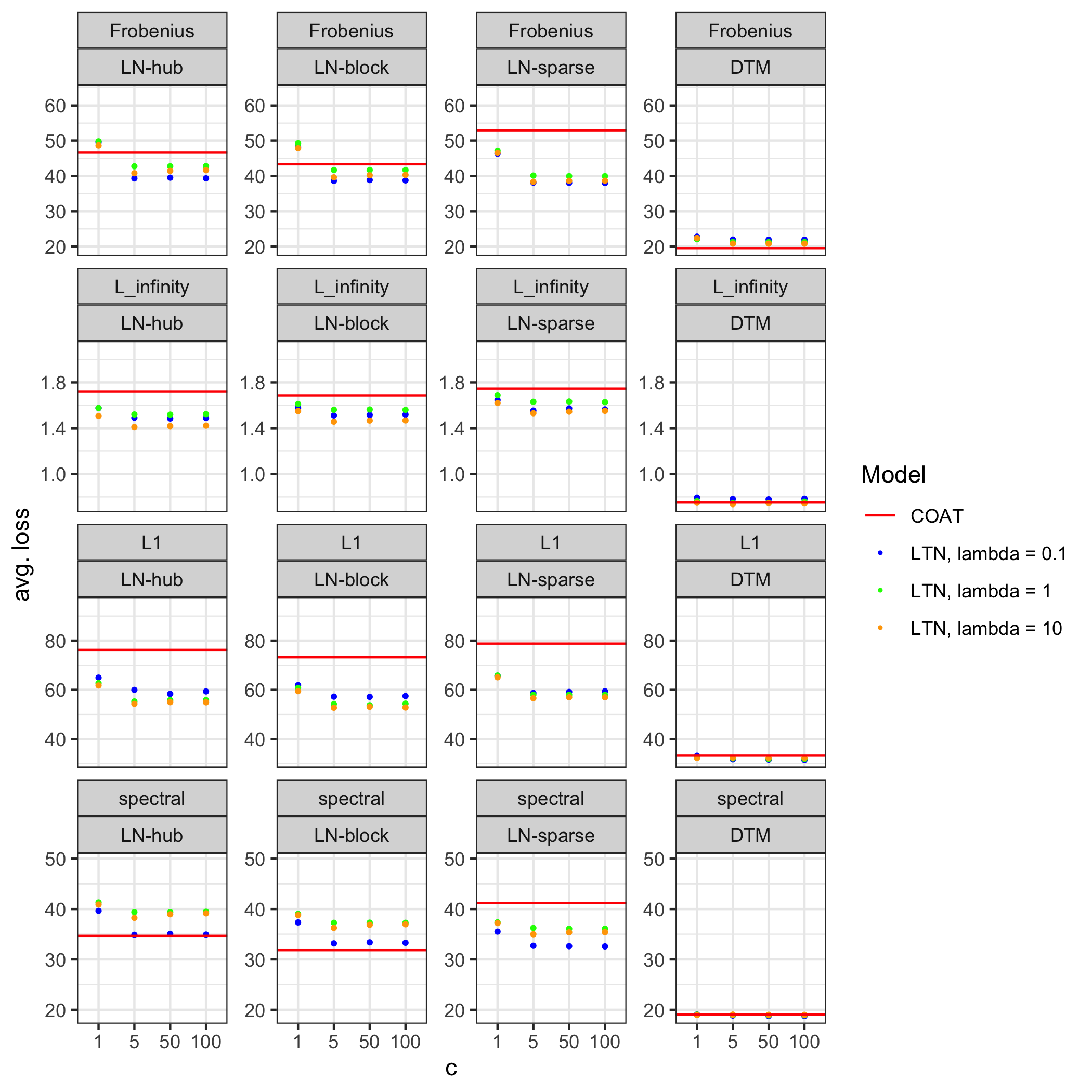
Figure S1: Comparisons of loss of two methods under LN and DTM simulation settings. $\lambda$ is the shrinkage parameter in graphical lasso prior, and the prior covariance of $\boldsymbol{\mu}$ is $c\boldsymbol{I}$

C Sensitivity analysis on tree misspecification

We investigate the robustness of the inference of mean and covariance structure to the choice of partition tree. Let ${\mathcal{T}_{1}}$ be a phylogenetic tree such that all of the right children of the internal nodes are leaves, ${\mathcal{T}_{2}}$ a balanced tree where the left and right subtree of each node have identical shape, and ${\mathcal{T}_{3}}$ the opposite of ${\mathcal{T}_{1}}$, where all of the left children of the internal nodes are leaves. The leaves of the three trees have the same order in the pre-order traversal trace. The data $\boldsymbol{X}_{n\times K}$ is generated from $\rm{LTN}_{{\mathcal{T}_{1}}}(\boldsymbol{\mu}_{1},\boldsymbol{\Sigma}_{1})$, where number of samples $n=200$, number of OTUs $K=64$, $\boldsymbol{\mu}_{1}=(2,\cdots,2),\boldsymbol{\Sigma}_{1}=\boldsymbol{I}$.

For each $\mathcal{T}_{j}(j=1,2,3)$, we fit ${\rm LTN}_{\mathcal{T}_{j}}$ on $\boldsymbol{X}$ to estimate the mean and covariance of the log-odds at the internal nodes of $\mathcal{T}_{j}$, and convert such estimates from the misspecified trees to the correct tree $\mathcal{T}_{1}$ through a similar procedure as in section A.2.

We ran 100 replicates under this simulation setting. The MSE of $\mu$ and marginal correlations on the original tree $\mathcal{T}_{1}$ averaged over the 63 internal nodes are shown in Figure S2. As expected, the estimates under the correct tree almost always have the smallest MSE. Inference under misspecified trees seem to be more sensitive to the hyperparameter $\lambda$ than the correct tree. Interestingly, the tree structure have different effects on the inference of mean and covariance structure, and the balanced tree does not necessarily outperform the opposite of the correct tree.

Figures S3 and S4 provide a closer inspection of the nodes. The estimated mean and marginal correlations of the shallow nodes are relatively robust to the misspecified trees. However, for some of the deepest nodes, estimates based on the incorrect trees have high bias. This is to some extent expected. There is enough data at the shallow nodes for LTN to have reasonable estimates of mean and covariance even under misspecified trees; however, as the counts get sparser at deeper nodes, the inference become more sensitive to the prior on the compositions, which is distorted by the misspecified tree. Also we note that for inference based on $\mathcal{T}_{3}$, the estimated marginal correlations seem to have slightly higher bias at the two most shallow nodes of $\mathcal{T}_{1}$. This might be due to that the mean and correlations at these nodes are reparameterized on $\mathcal{T}_{3}$ in a very ineffective manner, resulting in accumulated errors in estimations.

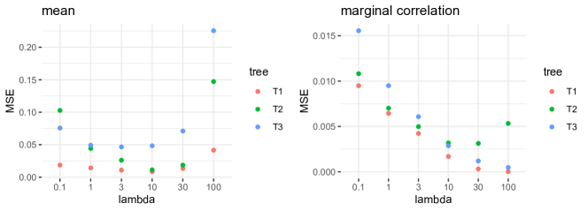
Figure S2: MSE of the estimated mean ($\boldsymbol{\mu}$) and marginal correlations on the original tree, averaged across all nodes. The MSE is calculated based on 100 replicates.

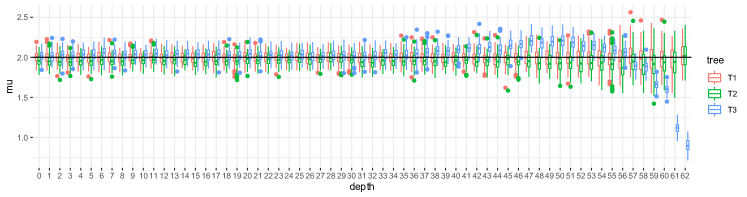
Figure S3: Estimated $\mu$ across nodes with $\lambda=10$. The boxplots are generated based on 100 replicates. The nodes are ordered by their depth in $\mathcal{T}_{1}$.

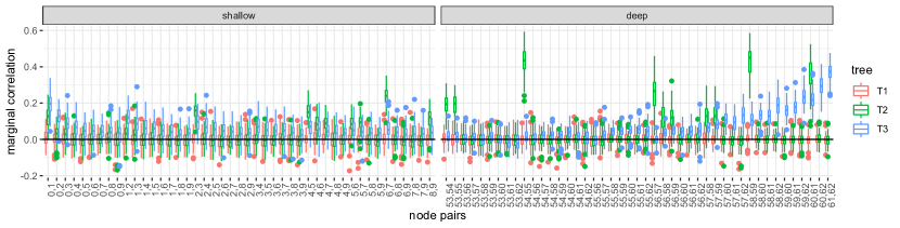
Figure S4: Estimated marginal correlations across nodes with $\lambda=10$. The left panel shows the shallowest ten nodes in $\mathcal{T}_{1}$ while the right shows the deepest ten nodes. The boxplots are generated based on 100 replicates. The nodes are labeled by their depth in $\mathcal{T}_{1}$.

D Additional figures and tables for case study

D.1 Covariates

Fig. S5 shows the multidimensional scaling results of the Bray-Curtis dissimilarity between samples, where age at collection increases almost in the same direction of the first axis, and the Finish and Estonian samples are roughly separated along the second axis in the case group. As shown in Fig. S6, the most abundant phylum has larger between-individual and within-individual variability at the very beginning of life, and stabilizes over time. For this reason, we take log transform of age to account for the more rapid changes in microbiome compositions at early age. Interestingly, seroconversion generally happens after the highly variable phase. Most samples collected after one year old are dominated with either Bacteroidetes or Firmicutes. Moreover, it is worth noting that Actinobacteria dominates other taxa in about half of the samples collected from Estonian individuals during the first year, while that’s not the case for Finnish individuals.

Figure S5: Multidimensional scaling of Bray-Curtis dissimilarity between samples

Figure S6: The most abundant phylum in each sample

D.2 PMAPs

(a)

(b)

Figure S7: (a) Relative abundance of distasonis. Data collected before the first event of seroconversion is omitted. (b) Relative abundance of OTU 4439360.

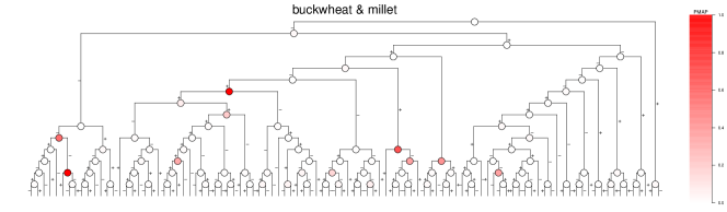
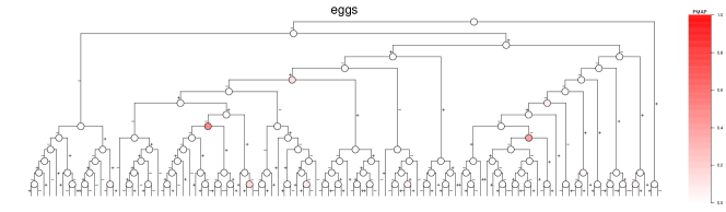
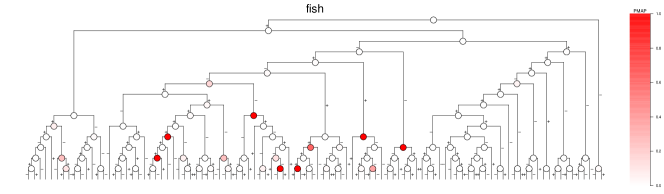
Figure S9: PMAPs of buckwheat & millet, eggs and fish.

Table S1: Nodes with PMAP$>0.5$ for breastfeeding

node	taxon in common	taxa on left	taxa on right	$\hat{\alpha}$
$A_{1}$	Bacteria	Proteobacteria, Actinobacteria	Firmicutes, Bacteroidetes	0.46
$A_{2}$	Actinobacteria	Actinobacteria	Coriobacteriia	0.98
$A_{3}$	Bifidobacterium	unclassified, longum, bifidum	adolescentis	1.40
$A_{4}$	Clostridiales	Lachnospiraceae, Veillonellaceae	Ruminococcaceae	1.06
$A_{5}$	Clostridiales	Lachnospiraceae	Veillonellaceae	-1.62
$A_{6}$	Lachnospiraceae	OTU 289734, OTU 4483337, OTU 2724175, OTU 4448492	OTU 4469576	1.03
$A_{7}$	Ruminococcaceae	Oscillospira, Faecalibacterium, Ruminococcus	unclassified	-1.14
$A_{8}$	Clostridiaceae	OTU 193672	OTU 3576174	-1.85
$A_{9}$	Streptococcus	OTU 4442130	OTU 4425214	1.54

References

- Äijö et al. (2017) Äijö, T., C. L. Müller, and R. Bonneau (2017, 09). Temporal probabilistic modeling of bacterial compositions derived from 16S rRNA sequencing. Bioinformatics 34(3), 372–380.
- Aitchison (1982) Aitchison, J. (1982). The statistical analysis of compositional data. Journal of the Royal Statistical Society. Series B (Methodological) 44(2), 139–177.
- Beghini et al. (2021) Beghini, F., L. J. McIver, A. Blanco-Míguez, L. Dubois, F. Asnicar, S. Maharjan, A. Mailyan, P. Manghi, M. Scholz, A. M. Thomas, M. Valles-Colomer, G. Weingart, Y. Zhang, M. Zolfo, C. Huttenhower, E. A. Franzosa, and N. Segata (2021, May). Integrating taxonomic, functional, and strain-level profiling of diverse microbial communities with biobakery 3. Elife 10.
- Brugman et al. (2006) Brugman, S., F. A. Klatter, J. T. J. Visser, A. C. M. Wildeboer-Veloo, H. J. M. Harmsen, J. Rozing, and N. A. Bos (2006). Antibiotic treatment partially protects against type 1 diabetes in the bio-breeding diabetes-prone rat. is the gut flora involved in the development of type 1 diabetes? Diabetologia 49(9), 2105–2108.
- Callahan et al. (2016) Callahan, B. J., P. J. McMurdie, M. J. Rosen, A. W. Han, A. J. A. Johnson, and S. P. Holmes (2016). Dada2: High-resolution sample inference from illumina amplicon data. Nature Methods 13(7), 581–583.
- Cao et al. (2019) Cao, Y., W. Lin, and H. Li (2019). Large covariance estimation for compositional data via composition-adjusted thresholding. Journal of the American Statistical Association 114(526), 759–772.
- Davis-Richardson et al. (2014) Davis-Richardson, A. G., A. N. Ardissone, R. Dias, V. Simell, M. T. Leonard, K. M. Kemppainen, J. C. Drew, D. Schatz, M. A. Atkinson, B. Kolaczkowski, J. Ilonen, M. Knip, J. Toppari, N. Nurminen, H. Hyöty, R. Veijola, T. Simell, J. Mykkänen, O. Simell, and E. W. Triplett (2014). Bacteroides dorei dominates gut microbiome prior to autoimmunity in finnish children at high risk for type 1 diabetes. Frontiers in Microbiology 5, 678.
- Dedrick et al. (2020) Dedrick, S., B. Sundaresh, Q. Huang, C. Brady, T. Yoo, C. Cronin, C. Rudnicki, M. Flood, B. Momeni, J. Ludvigsson, and E. Altindis (2020, 02). The role of gut microbiota and environmental factors in type 1 diabetes pathogenesis. Frontiers in endocrinology 11, 78–78.
- Dennis III (1991) Dennis III, S. Y. (1991). On the hyper-dirichlet type 1 and hyper-liouville distributions. Communications in Statistics - Theory and Methods 20(12), 4069–4081.
- Egozcue and Pawlowsky-Glahn (2016) Egozcue, J. J. and V. Pawlowsky-Glahn (2016, July). Changing the Reference Measure in the Simplex and its Weighting Effects. Austrian Journal of Statistics 45(4), 25–44.
- Egozcue et al. (2003) Egozcue, J. J., V. Pawlowsky-Glahn, G. Mateu-Figueras, and C. Barceló-Vidal (2003, April). Isometric Logratio Transformations for Compositional Data Analysis. Mathematical Geology 35(3), 279–300.
- Fehr et al. (2020) Fehr, K., S. Moossavi, H. Sbihi, R. C. T. Boutin, L. Bode, B. Robertson, C. Yonemitsu, C. J. Field, A. B. Becker, P. J. Mandhane, M. R. Sears, E. Khafipour, T. J. Moraes, P. Subbarao, B. B. Finlay, S. E. Turvey, and M. B. Azad (2020, Aug). Breastmilk feeding practices are associated with the co-occurrence of bacteria in mothers’ milk and the infant gut: the child cohort study. Cell Host Microbe 28(2), 285–297.
- Giongo et al. (2011) Giongo, A., K. A. Gano, D. B. Crabb, N. Mukherjee, L. L. Novelo, G. Casella, J. C. Drew, J. Ilonen, M. Knip, H. Hyöty, R. Veijola, T. Simell, O. Simell, J. Neu, C. H. Wasserfall, D. Schatz, M. A. Atkinson, and E. W. Triplett (2011). Toward defining the autoimmune microbiome for type 1 diabetes. The ISME Journal 5(1), 82–91.
- Grantham et al. (2017) Grantham, N., B. Reich, E. Borer, and K. Gross (2017, 03). Mimix: a bayesian mixed-effects model for microbiome data from designed experiments. Journal of the American Statistical Association.
- Gueimonde et al. (2007) Gueimonde, M., K. Laitinen, S. Salminen, and E. Isolauri (2007). Breast milk: a source of bifidobacteria for infant gut development and maturation? Neonatology 92(1), 64–66.
- Jara and Hanson (2011) Jara, A. and T. E. Hanson (2011, 09). A class of mixtures of dependent tail-free processes. Biometrika 98(3), 553–566.
- Kostic et al. (2015) Kostic, A. D., D. Gevers, H. Siljander, T. Vatanen, T. Hyötyläinen, A.-M. Hämäläinen, A. Peet, V. Tillmann, P. Pöhö, I. Mattila, H. Lähdesmäki, E. A. Franzosa, O. Vaarala, M. de Goffau, H. Harmsen, J. Ilonen, S. M. Virtanen, C. B. Clish, M. Orešič, C. Huttenhower, M. Knip, and R. J. Xavier (2015, 2020/12/18). The dynamics of the human infant gut microbiome in development and in progression toward type 1 diabetes. Cell Host & Microbe 17(2), 260–273.
- La Rosa et al. (2012) La Rosa, P. S., J. P. Brooks, E. Deych, E. L. Boone, D. J. Edwards, Q. Wang, E. Sodergren, G. Weinstock, and W. D. Shannon (2012). Hypothesis testing and power calculations for taxonomic-based human microbiome data. PloS one 7(12), e52078–e52078.
- Mao et al. (2020) Mao, J., Y. Chen, and L. Ma (2020). Bayesian graphical compositional regression for microbiome data. Journal of the American Statistical Association 115(530), 610–624.
- McArdle and Anderson (2001) McArdle, B. H. and M. J. Anderson (2001). Fitting multivariate models to community data: a comment on distance-based redundancy analysis. Ecology 82(1), 290–297.
- Polson et al. (2013) Polson, N. G., J. G. Scott, and J. Windle (2013). Bayesian inference for logistic models using pólya–gamma latent variables. Journal of the American Statistical Association 108(504), 1339–1349.
- Ren et al. (2020) Ren, B., S. Bacallado, S. Favaro, T. Vatanen, C. Huttenhower, and L. Trippa (2020, 03). Bayesian mixed effects models for zero-inflated compositions in microbiome data analysis. Ann. Appl. Stat. 14(1), 494–517.
- Silverman et al. (2017) Silverman, J., A. Washburne, S. Mukherjee, and L. David (2017, February). A phylogenetic transform enhances analysis of compositional microbiota data. eLife 6.
- Silverman et al. (2018) Silverman, J. D., H. K. Durand, R. J. Bloom, S. Mukherjee, and L. A. David (2018). Dynamic linear models guide design and analysis of microbiota studies within artificial human guts. Microbiome 6(1), 202.
- Stojanov et al. (2020) Stojanov, S., A. Berlec, and B. Štrukelj (2020, 11). The influence of probiotics on the firmicutes/bacteroidetes ratio in the treatment of obesity and inflammatory bowel disease. Microorganisms 8(11), 1715.
- Tang et al. (2018) Tang, Y., L. Ma, and D. L. Nicolae (2018). A phylogenetic scan test on a Dirichlet-tree multinomial model for microbiome data. The Annals of Applied Statistics 12(1), 1 – 26.
- Vatanen et al. (2016) Vatanen, T., A. D. Kostic, E. d’Hennezel, H. Siljander, E. A. Franzosa, M. Yassour, R. Kolde, H. Vlamakis, T. D. Arthur, A.-M. Hämäläinen, A. Peet, V. Tillmann, R. Uibo, S. Mokurov, N. Dorshakova, J. Ilonen, S. M. Virtanen, S. J. Szabo, J. A. Porter, H. Lähdesmäki, C. Huttenhower, D. Gevers, T. W. Cullen, M. Knip, D. S. Group, and R. J. Xavier (2016, 05). Variation in microbiome lps immunogenicity contributes to autoimmunity in humans. Cell 165(4), 842–853.
- Wang (2012) Wang, H. (2012, 12). Bayesian graphical lasso models and efficient posterior computation. Bayesian Anal. 7(4), 867–886.
- Xia et al. (2013) Xia, F., J. Chen, W. K. Fung, and H. Li (2013, December). A Logistic Normal Multinomial Regression Model for Microbiome Compositional Data Analysis: Logistic Normal Multinomial Regression. Biometrics 69(4), 1053–1063.
- Xiao et al. (2018) Xiao, J., L. Chen, Y. Yu, X. Zhang, and J. Chen (2018). A phylogeny-regularized sparse regression model for predictive modeling of microbial community data. Frontiers in Microbiology 9.
- Zhou et al. (2021) Zhou, F., K. He, Q. Li, R. S. Chapkin, and Y. Ni (2021, February). Bayesian biclustering for microbial metagenomic sequencing data via multinomial matrix factorization. Biostatistics.