Fast Bayesian Variable Selection in Binomial and Negative Binomial Regression

Abstract

Bayesian variable selection is a powerful tool for data analysis, as it offers a principled method for variable selection that accounts for prior information and uncertainty. However, wider adoption of Bayesian variable selection has been hampered by computational challenges, especially in difficult regimes with a large number of covariates or non-conjugate likelihoods. Generalized linear models for count data, which are prevalent in biology, ecology, economics, and beyond, represent an important special case. Here we introduce an efficient MCMC scheme for variable selection in binomial and negative binomial regression that exploits Tempered Gibbs Sampling (Zanella and Roberts, 2019) and that includes logistic regression as a special case. In experiments we demonstrate the effectiveness of our approach, including on cancer data with seventeen thousand covariates.

1 Introduction

Generalized linear models are ubiquitous throughout applied statistics and data analysis (McCullagh and Nelder, 2019). One reason for their popularity is their interpretability: they introduce explicit parameters that encode how the observed response depends on each particular covariate. In the scientific setting this interpretability is of central importance. Indeed model fit is often a secondary concern, and the primary goal is to identify a parsimonious explanation of the observed data. This is naturally viewed as a model selection problem, in particular one in which the model space is defined as a nested set of models, with distinct models including distinct sets of covariates.

The Bayesian formulation of this approach, known as Bayesian variable selection in the literature, offers a powerful set of techniques for realizing Occam’s razor in this setting (George and McCulloch, 1993, 1997; Chipman et al., 2001; Dellaportas et al., 2002; O’Hara et al., 2009). Despite the intuitive appeal of this approach, computing or otherwise approximating the resulting posterior distribution can be computationally challenging. A principal reason for this is the astronomical size of the model space that results whenever there are more than a few dozen covariates. Indeed for $P$ covariates the total number of distinct models, namely $2^{P}$, exceeds the estimated number of atoms in the known universe ($\sim\!10^{80}$) for $P\gtrsim 266$. In addition for most models of interest non-conjugate likelihoods make it infeasible to integrate out real-valued model parameters, resulting in a challenging high-dimensional inference problem defined on a transdimensional mixed discrete/continuous latent space.

In this work we develop efficient MCMC methods for Bayesian variable selection for two generalized linear models that are commonly used for analyzing count data: i) binomial regression (and its special case logistic regression); and ii) negative binomial regression. To enable efficient inference we proceed in two steps. First, we utilize Pòlya-Gamma auxiliary variables to establish conjugacy (Polson et al., 2013). Second, to enable targeted exploration of the high-dimensional model space we adapt the Tempered Gibbs Sampler (TGS) introduced by Zanella and Roberts (2019) to our setting. As we will see, this approach ensures that computational resources are strategically utilized to explore high probability regions of model space.

2 Bayesian variable selection in binomial regression

For simplicity we focus on the binomial regression case, leaving a discussion of the negative binomial case to Sec. A.5 in the supplemental materials. Let $X\in\mathbb{R}^{N\times P}$, $C\in\mathbb{Z}^{N}_{>0}$, and $Y\in\mathbb{Z}^{N}_{\geq 0}$ with $Y\leq C$ . We consider the following space of generalized linear models:

$${\rm[inclusion\;variables]}\qquad \gamma_{i}\sim{\rm Bernoulli}(h) {\rm for}\;\;i=1,...,P$$ (1)

$${\rm[bias\;term]}\qquad \beta_{0}\sim\mathcal{N}(0,\tau_{\rm bias}^{-1})$$

$${\rm[coefficients]}\qquad \beta_{\gamma}\sim\mathcal{N}(0,\tau^{-1}\mathbb{1}_{|\gamma|})$$

$${\rm[success\;logits]}\qquad \psi_{n}\equiv\beta_{0}+\beta_{\gamma}\cdot X_{n\gamma} {\rm for}\;\;n=1,...,N$$

$${\rm[responses]}\qquad Y_{n}\sim{\rm Binomial}(C_{n},\sigma(\psi_{n})) {\rm for}\;\;n=1,...,N$$

Here each $\gamma_{i}\in\{0,1\}$ controls whether the $i^{\rm th}$ coefficient $\beta_{i}$—and therefore the $i^{\rm th}$ covariate—is included ($\gamma_{i}=1$) or excluded ($\gamma_{i}=0$) from the model. In the following we use $\gamma$ to refer to the full $P$-dimensional vector $(\gamma_{1},...,\gamma_{P})$. The hyperparameter $h\in(0,1)$ controls the overall level of sparsity; in particular $hP$ is the expected number of covariates included a priori. The bias term is governed by a Normal prior with precision $\tau_{\rm bias}>0$. Likewise the $|\gamma|$ coefficients $\beta_{\gamma}\in\mathbb{R}^{|\gamma|}$ are governed by a Normal prior with precision $\tau>0$. For simplicity we take $\tau=\tau_{\rm bias}$ throughout. Here $|\gamma|\in\{0,1,...,P\}$ denotes the total number of included covariates. Note that we assume that the bias term $\beta_{0}$ is always included. The response $Y_{n}$ is generated from a Binomial distribution with total count $C_{n}$ and success probability $\sigma(\psi_{n})$, where $\sigma(\cdot)$ denotes the logistic or sigmoid function $\sigma(x)\equiv\{1+\exp(-x)\}^{-1}$. This reduces to conventional logistic regression with binary responses if $C_{n}=1$ for all $n$. In the following we drop the $\gamma$ subscript on $\beta_{\gamma}$ to simplify the notation.

3 Inference

3.1 Pòlya-Gamma augmentation

Introducing Pòlya-Gamma auxiliary variables is an example of data augmentation, which is commonly used to establish conjugacy or improve mixing (Tanner and Wong, 1987). Pòlya-Gamma augmentation relies on the identity

$$\frac{(e^{\psi})^{a}}{(1+e^{\psi})^{b}}=2^{-b}e^{(a-\tfrac{1}{2}b)\psi}\mathbb{E}_{{\rm PG}(\omega|b,0)}\left[\exp(-\tfrac{1}{2}\omega\psi^{2})\right]$$ (2)

noted by Polson et al. (2013). Here $a,\psi\in\mathbb{R}$, $b>0$, and ${\rm PG}(\omega|b,0)$ is the Pòlya-Gamma distribution, which has support on the positive real axis. Using this identity we can introduce a $N$-dimensional vector of Pòlya-Gamma variates $\omega$ governed by the prior $\omega_{n}\sim{\rm PG}(C_{n},0)$ and rewrite the Binomial likelihood in Eqn. 1 as follows

$$p(Y_{n}|C_{n},\sigma(\psi_{n}))\propto\sigma(\psi_{n})^{Y_{n}}(1-\sigma(\psi_{n}))^{C_{n}-Y_{n}}=\frac{(\exp(-\psi_{n}))^{C_{n}-Y_{n}}}{(1+\exp(-\psi_{n}))^{C_{n}}}=\frac{(\exp(\psi_{n}))^{Y_{n}}}{(1+\exp(\psi_{n}))^{C_{n}}}$$

so that each Binomial likelihood term in Eqn. 1 is now replaced with a factor

$$\exp(\kappa_{n}\psi_{n}-\tfrac{1}{2}\omega_{n}\psi_{n}^{2})\qquad{\rm with}\qquad\kappa_{n}\equiv Y_{n}-\tfrac{1}{2}C_{n}$$ (3)

This augmentation leaves the marginal distribution w.r.t. $(\gamma,\beta)$ unchanged. Crucially each factor in Eqn. 3 is Gaussian w.r.t. $\beta$, with the consequence that Pòlya-Gamma augmentation establishes conjugacy.

3.2 Binary variables and Metropolized-Gibbs

The augmented model in Sec. 3.1 readily admits a conventional Gibbs sampling scheme. However, the mixing time of the resulting sampler is notoriously slow in high dimensions: the sampler is sticky. For example, consider the scenario in which the two covariates corresponding to $i=1$ and $i=2$ are highly correlated and each on its own is sufficient for explaining the observed data. In this scenario the posterior concentrates on models with $\gamma=(1,0,0,0,...)$ and $\gamma=(0,1,0,0,...)$. Unfortunately, single-site Gibbs updates w.r.t. $\gamma_{i}$ will move between the two modes very infrequently, since they are separated by low probability models like $\gamma=(0,0,0,0,...)$ and $\gamma=(1,1,0,0,...)$.

To motivate the Tempered Gibbs Sampling (TGS) strategy that we use to deal with this stickiness, we consider a single latent binary variable $x$ governed by the probability distribution $p(x)={\rm Bernoulli}(q)$. A Gibbs sampler for this distribution simply samples $x\sim p$ in each iteration of the Markov chain. An alternative strategy is to employ a so-called Metropolized-Gibbs move w.r.t. $x$ (Liu, 1996). For binary $x$ this results in a proposal distribution that is deterministic in the sense that it always proposes a flip: $0\to 1$ or $1\to 0$. The corresponding Metropolis-Hastings (MH) acceptance probability for a proposed move $x\to x^{\prime}$ is given by

$$\alpha(x\!\to\!x^{\prime})=\begin{cases}\min(1,\tfrac{q}{1-q})&{\rm if}\;x=0\\ \min(1,\tfrac{1-q}{q})&{\rm if}\;x=1\end{cases}$$ (4)

As is well known, this update rule is more statistically efficient than the corresponding Gibbs move (Liu, 1996). For our purposes, however, what is particularly interesting is the special case where $q=\tfrac{1}{2}$. In this case the acceptance probability in Eqn. 4 is identically equal to one. Consequently the Metropolized-Gibbs chain is deterministic:

$$...\to 0\to 1\to 0\to 1\to 0\to 1\to...$$ (5)

Indeed this Markov chain can be described as maximally non-sticky.

3.3 A tempered inference scheme

We now describe how we adapt the Tempered Gibbs Sampling (TGS) strategy in Zanella and Roberts (2019) to our setting. The basic idea of TGS in this context is to introduce a tempered auxiliary target distribution that leverages the non-sticky dynamics described in Sec. 3.2. Importantly, this tempered distribution needs to be sufficiently close to the PG-augmented distribution described in Sec. 3.1 so that we can use importance sampling to obtain samples from the PG-augmented distribution while avoiding high-variance importance weights.

In more detail we proceed as follows. The augmented target distribution in Sec. 3.1 is given by

$$p(Y|\beta,\gamma,\omega,X,C)p(\beta)p(\gamma)p(\omega|C) =Zp(\beta,\gamma,\omega|\mathcal{D})$$ (6)

where we define $\mathcal{D}\equiv\{X,Y,C\}$ so that $p(\beta,\gamma,\omega|\mathcal{D})$ is the corresponding posterior and $Z$ is the (intractable) normalization constant. Since the dimension of $\beta$ depends on $\gamma$, it is advantageous to marginalize out $\beta$ to obtain

$$p(Y|\gamma,\omega,X,C)p(\gamma)p(\omega|C)=Zp(\gamma,\omega|\mathcal{D})$$ (7)

Thanks to Pòlya-Gamma augmentation we can compute $p(Y|\gamma,\omega,X,C)$ in closed form. The next step is to induce coordinatewise tempering in Eqn. 7. To do this we introduce an auxiliary variable $i\in\{0,1,2,...,P\}$ that controls which variables, if any, are tempered. In particular we define the following tempered (unnormalized) target distribution:

$$f(\gamma,\omega,i) \equiv Zp(\gamma,\omega|\mathcal{D})\left\{\delta_{i0}\xi+\frac{1}{P}\sum_{j=1}^{P}\delta_{ij}\eta(\gamma_{-j},\omega)\frac{U(\gamma_{j})}{p(\gamma_{j}|\gamma_{-j},\omega,\mathcal{D})}\right\}$$ (8)

$$=\delta_{i0}\xi Zp(\gamma,\omega|\mathcal{D})+\frac{Z}{P}\sum_{j=1}^{P}\delta_{ij}\eta(\gamma_{-j},\omega)U(\gamma_{j})p(\gamma_{-j},\omega|\mathcal{D})$$

Here $\xi>0$ is a hyperparameter whose choice we discuss below and $\delta_{ij}$ is the Kronecker delta. Furthermore $U(\cdot)$ is the uniform distribution on $\{0,1\}$ and $\gamma_{-j}$ denotes all components of $\gamma$ apart from $\gamma_{j}$. Finally $\eta(\gamma_{-j},\omega)$ is an additional weighting factor to be defined later; for now the reader can suppose that $\eta(\gamma_{-j},\omega)=1$.

We note three important features of Eqn. 8. First, since $i$ is included explicitly as a variable in Eqn. 8 we can use $i$ to guide our sampling strategy without violating the conditions of a Markov chain. Second, by construction when $i>0$ the posterior conditional w.r.t. $\gamma_{i}$ is the uniform distribution $U(\gamma_{i})$. Consequently for $i>0$ Metropolized-Gibbs updates w.r.t. $\gamma_{i}$ will result in the desired non-sticky dynamics described in the previous section. Third, as we discuss in more detail in Sec. A.1, the posterior conditional $p(\gamma_{i}|\gamma_{-i},\omega,\mathcal{D})$ in Eqn. 8 can be computed in closed form thanks to Pòlya-Gamma augmentation. This is important because computing $p(\gamma_{i}|\gamma_{-i},\omega,\mathcal{D})$ is necessary for importance weighting as well as computing Rao-Blackwellized posterior inclusion probabilities.

We proceed to construct a sampling scheme for the target distribution Eqn. 8 that utilizes Gibbs updates w.r.t. $i$, Metropolized-Gibbs updates w.r.t. $\gamma_{i}$, and Metropolis-Hastings updates w.r.t. $\omega$.

$i$-updates

If we marginalize $i$ from Eqn. 8 we obtain

$$f(\gamma,\omega)=Zp(\gamma,\omega|\mathcal{D})\left\{\xi+\frac{1}{P}\sum_{j=1}^{P}\eta(\gamma_{-j},\omega)\frac{U(\gamma_{j})}{p(\gamma_{j}|\gamma_{-j},\omega,\mathcal{D})}\right\}=Zp(\gamma,\omega|\mathcal{D})\phi(\gamma,\omega)$$ (9)

where we define

$$\phi(\gamma,\omega)\equiv\xi+\frac{1}{P}\sum_{i=1}^{P}\frac{\tfrac{1}{2}\eta(\gamma_{-i},\omega)}{p(\gamma_{i}|\gamma_{-i},\omega,\mathcal{D})}$$ (10)

As is clear from Eqn. 9, $\phi(\gamma,\omega)^{-1}$ is the importance weight that is used to obtain samples from the non-tempered target Eqn. 7. Additionally these equations imply that we can do Gibbs updates w.r.t. $i$ using the (normalized) distribution

$$f(i|\gamma,\omega)=\frac{1}{\phi(\omega,\gamma)}\left(\delta_{i0}\xi+\frac{1}{P}\sum_{j=1}^{P}\delta_{ij}\frac{\tfrac{1}{2}\eta(\gamma_{-j}|\omega)}{p(\gamma_{j}|\gamma_{-j},\omega,\mathcal{D})}\right)$$ (11)

To better understand the behavior of the auxiliary variable $i$, we compute the marginal distribution w.r.t. $i$ for the special case $\eta(\cdot)=1$:

$$f(i)\propto\delta_{i0}\xi+\frac{1}{P}\sum_{j=1}^{P}\delta_{ij}$$ (12)

We can read off several conclusions from Eqn. 12. First, $\xi$ controls how frequently we visit the $i=0$ state. Second, if $\eta(\cdot)=1$ then the states with $i>0$ (each of which corresponds to a particular covariate in X) are visited equally often. Later we discuss how we can choose $\eta(\cdot)$ to preferentially visit certain states and thus preferentially update $\gamma_{i}$ for particular covariates.

$\gamma$-updates

Whenever $i>0$ we update $\gamma_{i}$. As discussed above, for $i>0$ the posterior conditional w.r.t. $\gamma_{i}$ is the uniform distribution $U(\gamma_{i})$. We employ Metropolized-Gibbs updates w.r.t. $\gamma_{i}$, resulting in deterministic flips that are accepted with probability one: $\gamma_{i}\to 1-\gamma_{i}$.

$\omega$-updates

Whenever $i=0$ we update $\omega$. To do so we use a simple proposal distribution that can be computed in closed form. Importantly $f(\gamma,\omega,i=0)$ is not tempered so we can rely on the conjugate structure that is made manifest when we condition on an explicit value of $\beta$. In more detail, we first compute the mean of the conditional posterior distribution $p(\beta|\gamma,\omega,\mathcal{D})$ of Eqn. 6:

$$\hat{\beta}(\gamma,\omega)\equiv\mathbb{E}_{p(\beta|\gamma,\omega,\mathcal{D})}\left[\beta\right]$$ (13)

Using this (deterministic) value we then form the conditional posterior distribution $p(\omega^{\prime}|\gamma,\hat{\beta},\mathcal{D})$, which is a Pòlya-Gamma distribution whose parameters are readily computed. We then sample a proposal $\omega^{\prime}\sim p(\cdot|\gamma,\hat{\beta},\mathcal{D})$ and compute the corresponding MH acceptance probability $\alpha(\omega\!\to\!\omega^{\prime}|\gamma)$. The proposal is then accepted with probability $\alpha(\omega\!\to\!\omega^{\prime}|\gamma)$; otherwise it is rejected. The acceptance probability can be computed in closed form and is given by

$$\!\!\!\alpha(\omega\!\to\!\omega^{\prime}|\gamma) =\min\!\left(\!1,\frac{p(Y|\gamma,\omega^{\prime},X,C)}{p(Y|\gamma,\omega,X,C)}\frac{p(Y|\gamma,\omega,\hat{\beta}(\gamma,\omega^{\prime}),X,C)}{p(Y|\gamma,\omega^{\prime},\hat{\beta}(\gamma,\omega),X,C)}\frac{p(Y|\gamma,\hat{\beta}(\gamma,\omega),X,C)}{p(Y|\gamma,\hat{\beta}(\gamma,\omega^{\prime}),X,C)}\right)$$ (14)

Each of the terms in Eqn. 14 can be readily computed; conveniently there is no need to compute the Pòlya-Gamma density, which can be challenging in some regimes. See Sec. A.3 for more details.

We note that the proposal distribution $p(\omega^{\prime}|\gamma,\hat{\beta}(\gamma,\omega),\mathcal{D})$ can be thought of as an approximation to the posterior conditional $p(\omega^{\prime}|\gamma,\mathcal{D})=\int\!d\beta\,p(\omega^{\prime}|\gamma,\beta,\mathcal{D})p(\beta|\gamma,\mathcal{D})$ that would be used in a Gibbs update. Since this latter density is intractable, we instead opt for this tractable option. One might worry that the resulting acceptance probability would be very low, since $\omega$ is $N$-dimensional and $N$ can be large. However, $p(\omega^{\prime}|\gamma,\beta,\mathcal{D})$ only depends on $\beta$ through the scalars $\psi_{n}=\beta_{\gamma}\cdot X_{n\gamma}$; the induced posterior over $\psi_{n}$ is typically somewhat narrow, since the $\psi_{n}$ are pinned down by the observed data, and consequently $p(\omega^{\prime}|\gamma,\hat{\beta},\mathcal{D})$ is a reasonably good approximation to the exact posterior conditional. In practice we observe high mean acceptance probabilities $\sim 50\%-95\%$ for all the experiments in this work, even for $N\gg 10^{2}$, although we note that we would expect problematically small acceptance probabilities in sufficiently extreme regimes, for example if both $N$ and $C$ are large.

Weighting factor $\eta$

To finish specifying our inference scheme we need to choose the weighting factor $\eta(\gamma_{-j},\omega)$ in Eqn. 8. As discussed after Eqn. 12, if we choose $\eta(\cdot)=1$ the $P$ states corresponding to $i>0$ will be explored with equal frequency. For covariates $i$ that have very small posterior inclusion probabilities (PIPs), i.e. $p(\gamma_{i}=1|\mathcal{D})\ll 1$, this non-preferential exploration strategy will tend to waste computation on exploring parts of $\gamma$ space with low posterior probability. By choosing $\eta(\cdot)$ accordingly we can steer our computational resources towards high probability regions of the posterior. Similarly to Zanella and Roberts (2019) we let

$$\eta(\gamma_{-j},\omega)=p(\gamma_{j}=1|\gamma_{-j},\omega)+\tfrac{\epsilon}{P}$$ (15)

Here $p(\gamma_{j}=1|\gamma_{-j},\omega)$ is a conditional PIP, and $\epsilon$ is a hyperparameter that trades off between exploitation ($\epsilon\to 0$) and exploration ($\epsilon\to\infty$).

For the full algorithm see Algorithm 1. Following Zanella and Roberts (2019) we call the algorithm with trivial $\eta(\cdot)$ TGS and the algorithm with non-trivial $\eta(\cdot)$ Weighted TGS (wTGS). Furthermore we call the algorithm without tempering but with $\eta(\cdot)$ as in Eqn. 15 wGS. Like (w)TGS this algorithm utilizes Metroplized-Gibbs moves w.r.t. $\gamma_{i}$, although in contrast to (w)TGS the $\gamma_{i}$ update is not deterministic.

Input: Dataset $\mathcal{D}=\{X,Y,C\}$ with $N$ data points and $P$ covariates; total number of MCMC iterations $T$; number of burn-in iterations $T_{\rm burn}$; hyperparameter $\xi>0$ (optional)

Output: Approximate weighted posterior samples $\{\rho_{t},\gamma_{t},\omega_{t}\}^{T}_{t=T_{\rm burn}+1}$

1 Let $\gamma_{0}=(0,...,0)$ and $\omega_{0}\sim{\rm PG}(C,0)$.

2 for $t=1,...,T$ do

3       Sample $i_{t}\sim f(\cdot|\gamma_{t-1},\omega_{t-1})$ using Eqn. 11

4       If $i_{t}>0$ let $\gamma_{t}={\rm flip}(\gamma_{t-1}|i_{t})$ where ${\rm flip}(\gamma|i)$ flips the $i^{\rm th}$ coordinate of $\gamma$: $\gamma_{i}\to 1-\gamma_{i}$.

5       Otherwise if $i_{t}=0$ sample $\omega_{t}^{\prime}\sim p(\cdot|\gamma_{t-1},\hat{\beta}(\gamma_{t-1},\omega_{t-1}),\mathcal{D})$. Set $\omega_{t}=\omega_{t}^{\prime}$ with probability $\alpha(\omega\!\to\!\omega^{\prime}|\gamma)$ given in Eqn. 14. Otherwise set $\omega_{t}=\omega_{t-1}$.

6       Compute the unnormalized weight $\tilde{\rho}_{t}=\phi(\gamma_{t},\omega_{t})^{-1}$ using Eqn. 10.

7       If $\xi$ is not provided and $t\leq T_{\rm burn}$ adapt $\xi$ using the scheme described in Sec. A.4.

8Compute the normalized weights $\rho_{t}=\frac{\tilde{\rho}_{t}}{\sum_{s>T_{\rm burn}}\tilde{\rho}_{s}}$ for $t=T_{\rm burn}+1,...,T$.

return $\{\rho_{t},\gamma_{t},\omega_{t}\}_{t=T_{\rm burn}+1}^{T}$

Algorithm 1 We outline the main steps in (w)TGS. wTGS uses the weighting function $\eta(\cdot)$ in Eqn. 15 and TGS uses $\eta(\cdot)=1$. See Sec. 3 for details.

Importance weights

The Markov chain in Algorithm 1 targets the auxiliary distribution Eqn. 8. To obtain samples from the desired posterior $p(\gamma,\omega|\mathcal{D})$ we must reweight each sample $(\gamma,\omega)$ with an importance weight given by $\rho=\phi(\gamma,\omega)^{-1}$; see Eqn. 9. Crucially, for TGS with $\eta(\cdot)=1$ we necessarily have $\rho\leq(\xi+\tfrac{1}{2})^{-1}$. Likewise for wTGS we necessarily have $\rho\leq(\xi+\tfrac{\epsilon}{2P})^{-1}$. We typically choose a value for $\xi$ in the range $\xi\sim 1-5$. Consequently the importance weights $\rho$ are bounded from above by a $\mathcal{O}(1)$ constant and exhibit only moderate variance. Ultimately this moderate variance can be traced to the coordinatewise tempering scheme used in TGS, which keeps the tempering to a modest level. Nevertheless as we show in experiments in Sec. 5, this modest amount of tempering leads to dramatic improvements in statistical efficiency.

4 Related work

Some of the earliest approaches to Bayesian variable selection (BVS) were introduced by George and McCulloch (1993, 1997). Chipman et al. (2001) provide an in-depth discussion of BVS for linear regression and CART models. Zanella and Roberts (2019) introduce Tempered Gibbs Sampling (TGS) and apply it to BVS for linear regresion. Nikooienejad et al. (2016) and Shin et al. (2018) advocate the use of non-local priors in the BVS setting. (Garcia-Donato and Martinez-Beneito, 2013) compare non-MCMC search methods for BVS to MCMC-based methods. Griffin et al. (2021) introduce an efficient adaptive MCMC method for BVS in linear regression. Wan and Griffin (2021) extend this approach to logistic regression and accelerated failure time models. We include this approach (ASI) in our empirical validation in Sec. 5. Tian et al. (2019) introduce an approach to BVS for logistic regression that relies on joint credible regions. Lamnisos et al. (2009) develop transdimensional MCMC chains for BVS in probit regression. Dellaportas et al. (2002) and O’Hara et al. (2009) review various methods for BVS. Polson et al. (2013) introduce Pòlya-Gamma augmentation and use it to develop efficient Gibbs samplers.

5 Experiments

In this section we validate the performance of Algorithm 1 on synthetic and real world data. We implement all algorithms using PyTorch (Paszke et al., ) and leverage the polyagamma package for sampling from Pòlya-Gamma distributions (Bleki, 2021). Besides our main algorithm wTGS, we consider its two simpler variants TGS and wGS. In addition we compare to ASI (Wan and Griffin, 2021), an adaptive MCMC scheme for logistic (and thus binomial) regression that likewise uses Pòlya-Gamma augmentation. In Sec. 5.1-5.3 we consider binomial and logistic regression and in Sec. 5.4-5.5 we consider negative binomial regression.

5.1 Runtime

In Fig. 1 we depict MCMC iteration times for wTGS for various values of $N$ and $P$. To make the benchmark realistic we use semi-synthetic data derived from the DUSP4 cancer dataset ($N=907$, $P=17273$) used in Sec. 5.3. As discussed in more detail in Sec. A.2 in the supplemental materials, all four algorithms have similar runtimes, since each is dominated by the $\mathcal{O}(P)$ cost of computing $p(\gamma_{j}=1|\gamma_{-j},\omega)$ for $j=1,...,P$. As can be seen in Fig. 1 for any given $N$ the iteration time is lower on CPU for small $P$, but GPU parallelization is advantageous for sufficiently large $P$. We also note that the computational complexity of wTGS is no worse than linear in $N$, with the consequence that wTGS can be applied to datasets with large $N$ and large $P$ in practice, at least if the sparsity assumption holds (i.e. most variables are excluded in the posterior: ${|\gamma|}\ll P$).

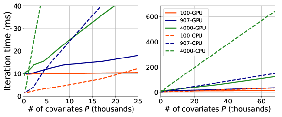
Figure 1: We depict MCMC iteration times in milliseconds for wTGS on CPU and GPU as the number of covariates $P$ is varied. We also vary the number of data points $N\in\{100,907,4000\}$. See Sec. 5.1 for details. Note that the figure on the left is a magnified version of the figure on the right. The CPU has 24 cores (Intel Xeon Gold 5220R 2.2GHz) and the GPU is a NVIDIA Tesla K80 GPU.

5.2 Correlated covariates scenario

We consider simulated datasets in which two covariates ($i=1$ and $i=2$) are highly-correlated and each on its own is able to fully explain the response $Y$. As discussed in Sec. 3.2 this can be a challenging regime for MCMC methods, since it is easy for the MCMC chain to get stuck in one mode and fail to explore the other mode. We consider four datasets with $(N,P)\in\{(32,32),(128,128),(512,1024),(512,4096)\}$. Each dataset has $C_{n}=10$ for all data points. See Fig. 2 and Fig. 3 for the results.

We see that wGS does poorly on all datasets, including the smallest one with $P=32$ covariates. By contrast wTGS yields low-variance PIP estimates in all cases. TGS does well for $P=32$ and $P=128$ but exhibits large variance for $P\geq 1024$. Together these results demonstrate the benefit of the non-sticky dynamics enabled by tempering, which allows (w)TGS to make frequent moves between the two modes. Comparing wTGS to TGS we see that the targeted $i$-updates enabled by $\eta(\cdot)$ further lower variance, especially for larger $P$. ASI estimates exhibit low variance for $P=32$ (apart from a single outlier) but are high variance for larger $P$. This outcome is easy to understand. Since ASI adapts its proposal distribution during warmup using a running estimate of each PIP, it is vulnerable to a rich-get-richer phenomenon in which covariates with large initial PIP estimates tend to crowd out covariates with which they are highly correlated. In the present scenario the result is that the ASI PIP estimates for the first two covariates are strongly anti-correlated. That this anti-correlation is ultimately due to suboptimal adaptation is easily verified. For example for $P=1024$ ($P=4096$) the Pearson correlation coefficient between the difference of final PIP estimates, i.e. PIP(1) - PIP(2), and the difference of the corresponding initial PIP estimates that define the proposal distribution is $0.904$ ($0.998$), respectively.

Figure 2: We depict posterior inclusion probability (PIP) estimates for the first covariate in the scenario described in Sec. 5.2 for four different MCMC methods. We depict results for $(N,P)=(32,32)$ [left] and $(N,P)=(128,128)$ [right]. At each iteration $t$ the PIP is computed using all samples obtained through iteration $t$. The mean PIP is depicted with a solid black line and light and dark grey confidence intervals denote $10\%\!-\!90\%$ and $30\%\!-\!70\%$ quantiles, respectively. The true PIP is almost exactly $\tfrac{1}{2}$. In each case we run 100 independent chains. For each method we also report the final PIP estimate (mean and standard deviation) in parentheses.

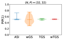
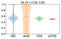
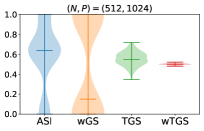
Figure 3: We depict violin plots for PIP estimates for the first covariate obtained with $10^{5}$ MCMC samples for four different methods on four datasets with varying numbers of data points $N$ and covariates $P$. Horizontal bars denote the minimum, median, and maximum PIP estimates obtained from 100 independent MCMC runs. See Sec. 5.2 for details.

5.3 Cancer data

We consider data from the Cancer Dependency Map project (Meyers et al., 2017; Behan et al., 2019; Pacini et al., 2021; DepMap, 2019a, b). This dataset includes 900+ cancer cell lines spanning 26 different tissue types. Each cell line has been subjected to a loss-of-function genetic screen that leverages CRISPR-Cas9 genetic editing to identify genes essential for cancer proliferation and survival. Genes identified by such screens are thought to be promising candidates for genetic vulnerabilities that can be used to guide the development of treatment strategies and novel therapeutics.

In more detail, we consider a subset of the data that includes $N=907$ cell lines and $P=17273$ covariates, with each covariate encoding the RNA expression level for a given gene. We consider two gene knockouts: DUSP4 and HNF1B. We make this choice because it is known that for both knockouts the RNA expression level of the corresponding gene is highly predictive of cell viability—this serves as a useful sanity check of our results. For each knockout the dataset contains a real-valued response that encodes the effect size of knocking out that particular gene. This response variable has a heavy tail that skews left; this tail corresponds to the small number of cancer cell lines for which the gene knockout has a large detrimental effect on cell viability and reflects the significant variability among different cell lines. We binarize this response variable by using the 20% quantile as a cutoff.

A minimum requirement for Bayesian variable selection to be useful in this setting is that results are reproducible across different MCMC runs. In Fig. 4 we depict the results we obtain from running pairs of independent MCMC chains for $2.5\times 10^{5}$ iterations after a burn-in of $2.5\times 10^{4}$ iterations. We see that the wTGS estimates show significantly more concordance between runs than is the case for ASI. For example, if we look at genes for which the PIP estimate for the DUSP4 dataset is at least $0.01$ ($0.10$) in at least one chain and compute inter-chain PIP ratios, then the maximum discrepancy for wTGS is $3.15$ ($1.33$), while the maximum discrepancy for ASI is $76.77$ ($12.79$), respectively. The corresponding numbers for HNF1B are $2.59$ ($1.35$) for wTGS and $40.19$ ($26.91$) for ASI.

What makes this dataset particularly challenging for analysis is that the $P=17273$ covariates are strongly correlated. For example, the DUSP4 RNA expression level exhibits a correlation greater than $0.40$ ($0.30)$ with $19$ ($203$) other covariates, respectively. Indeed the MIA covariate identified by both algorithms (see Fig. 4) exhibits a $0.43$ correlation with DUSP4, while PPP2R3A exhibits a $0.43$ correlation with KRT80. Similarly the HNF1B RNA expression level has a correlation greater than $0.70$ ($0.50)$ with $2$ ($33$) other covariates, respectively. This is typical for these kinds of datasets, since similar cell types employ similar cellular ‘programs.’

The runtime for each wTGS chain in Fig. 4 is $\sim\!70$ minutes on a NVIDIA Tesla K80 GPU. To obtain a much lower variance result we run wTGS for $\sim\!24$ hours and obtain $5\times 10^{6}$ samples. In Fig. 5 we confirm that the good concordance exhibited by wTGS PIP estimates obtained from chains with $2.5\times 10^{5}$ samples reflects the lower variance of wTGS PIP estimates as compared to ASI estimates. See Table 1 in the supplemental materials for a list of all the top hits.

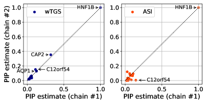
Figure 4: We depict PIP estimates for two independent MCMC chains for two cancer datasets (left: DUSP4; right: HNF1B) using two MCMC methods. For each method we depict the top 20 PIPs from chain #1 paired with the estimate from chain #2. The wTGS estimates show much better inter-chain concordance. For example, the PIPs obtained with ASI for KRT7 on the DUSP4 dataset (marked with a purple caret ^) differ by a factor of $12.8$ between the two chains, while the two wTGS estimates are $0.025$ and $0.021$. Similarly the PIPs obtained with ASI for C12orf54 on the HNF1B dataset differ by a factor of 26.9, while the two wTGS estimates are $0.113$ and $0.152$. See Sec. 5.3 for details.

Figure 5: In this companion figure to Fig. 4 we compare PIP estimates obtained from short wTGS and ASI chains with $2.5\times 10^{5}$ samples to a long wTGS chain with $5\times 10^{6}$ samples. For each method we depict the top 20 PIPs from the long chain paired with estimates from the short chains (top row: chain #1; bottom row: chain #2). The wTGS estimates obtained with the short chains are significantly more accurate than is the case for ASI. See Sec. 5.3 for details.

5.4 Hospital data

We consider a hospital visit dataset with $N=1798$ considered in (Hilbe, 2011) and gathered from Arizona Medicare data. The response variable is length of hospital stay for patients undergoing a particular class of heart procedure and ranges between 1 and 53 days. We expect the hospital stay to exhibit significant dispersion and so we use a negative binomial likelihood. There are three binary covariates: sex (female/male), admission type (elective/urgent), and age (over/under 75). To make the analysis more challenging we add 97 superfluous covariates drawn i.i.d. from a unit Normal distribution so that $P=100$.

Running wTGS on the full dataset we find strong evidence for inclusion of two of the covariates: sex (PIP $\approx 0.95$) and admission type (PIP $\approx 1.0$). The corresponding coefficients are negative ($-0.15\pm 0.02$) and positive ($0.63\pm 0.03$), respectively. This corresponds to shorter hospital stays for males and longer hospital stays for urgent admissions. In Fig. 6 (left) we depict trace plots for a few latent variables, each of which is consistent with good mixing.

Next we hold-out half of the dataset in order to assess the quality of the model-averaged predictive distribution. We use the mean predicted hospital stay to rank the held-out patients and then partition them into two groups of equal size. Comparing this predicted partition to the observed partition of patients into short- and long-stay patients, we find a classification accuracy of 66.6%. In Fig. 6 (right) we depict a more fine-grained predictive diagnostic, namely Dawid’s Probability Integral Transform (PIT) (Dawid, 1984). Since the PIT values are approximately uniformly distributed, we conclude that the predictive distribution is reasonably well-calibrated, although probably somewhat overdispersed.

Figure 6: Left: We depict trace plots for $\log(\nu)$ and two randomly chosen Pòlya-Gamma variates $\omega_{1}$ and $\omega_{2}$ for a wTGS run on the hospital data in Sec. 5.4. As expected the data is quite dispersed, with the posterior mean of the dispersion parameter $\nu$ being about $5.4$. Right: We depict the Probability Integral Transform histogram for $899$ held-out test points for the hospital data in Sec. 5.4.

5.5 Health survey data

We consider the German health survey with $N=1127$ considered in (Hilbe and Greene, 2007). The response variable is the annual number of visits to the doctor and ranges from $0$ to $40$ with a mean of $2.35$. As in Sec. 5.4, we expect significant dispersion and thus use a negative binomial likelihood. There are two covariates: i) a binary covariate for self-reported health status (not bad/bad); and ii) an age covariate, which ranges from 20 to 60. To make the analysis more challenging we add 198 superfluous covariates drawn i.i.d. from a unit Normal distribution so that $P=200$.

Running wTGS on the full dataset we find strong evidence for inclusion of the health status covariate (PIP $\approx 1.0$) and only marginal evidence for including age (PIP $\approx 0.08$). The health status coefficient is positive ($1.15\pm 0.10$), suggesting that patients whose health is self-reported as bad have $e^{1.15}\approx 3.17$ times as many visits to the doctor as compared to those who report otherwise. We find that the data are very overdispersed and infer the dispersion parameter to be $\nu=0.99\pm 0.07$. See Sec. A.5 for additional details on wTGS for negative binomial regression.

6 Discussion

Several possible improvements to wTGS as outlined above suggest themselves. A natural direction would be to combine the strengths of wTGS and ASI. Indeed one of the attractive features of ASI (Griffin et al., 2021; Wan and Griffin, 2021) is that the proposal enables moderately large moves in $\gamma$ space, i.e. not just single-site moves. Thus one possibility would be to incorporate such moves into wTGS, perhaps interleaving them with the wTGS moves. Alternatively, one could make ASI more like wTGS. In particular one could initialize the ASI proposal distribution using PIP estimates obtained with wTGS. This should help alleviate the difficulty with highly-correlated covariates exhibited by ASI in experiments in Sec. 5.2-5.3.

An additional challenge is the binomial regression regime with large $N$ and large $C$. As mentioned in Sec. 3.3, $\omega$-updates may suffer from low acceptance probabilities in this regime. Finding a suitably robust proposal distribution for this case remains an open problem.

More broadly, one of the principle challenges with Bayesian variable selection in the highly-correlated setting beyond inference itself is that of interpretation. How can one best convey to a user a manageable set of parsimonious models that are supported by the data? In scenarios with a large number of highly-correlated covariates, as is common for example in much of biology, posteriors that exhibit marginal evidence for a large number of highly-correlated covariates are inherently difficult to interpret. While this issue is common to Bayesian variable selection in all generalized linear models and not just (negative) binomial regression, better methods for making sense of complex high-dimensional posteriors are essential if Bayesian model selection is to find wider use among data analysts and scientists alike.

Appendix A Appendix

This appendix is organized as follows. In Sec. A.1 we discuss conditional marginal log likelihood computations. In Sec. A.2 we discuss computational complexity. In Sec. A.3 we discuss $\omega$-updates. In Sec. A.4 we discuss $\xi$ adapation. In Sec. A.5 we discuss the modifications of our basic algorithm that are needed to accommodate negative binomial likelihoods. In Sec. A.6 we include additional figures and tables accompanying Sec. 5. In Sec. A.7 we discuss experimental details.

A.1 Efficient linear algebra for the (conditional) marginal log likelihood

The conditional marginal log likelihood $\log p(Y|X,C,\gamma,\omega)$ can be computed in closed form where, up to irrelevant constants, we have

$$\log p(Y|X,C,\gamma,\omega) =\tfrac{1}{2}\mathcal{Z}_{\gamma+1}^{\rm T}(X_{\gamma+1}^{\rm T}\Omega X_{\gamma+1}+\tau\mathbb{1}_{\gamma+1})^{-1}\mathcal{Z}_{\gamma+1}$$ (16)

$$-\tfrac{1}{2}\log\det(X_{\gamma+1}^{\rm T}\Omega X_{\gamma+1}+\tau\mathbb{1}_{\gamma+1})-\tfrac{1}{2}\log\det(\tau^{-1}\mathbb{1}_{\gamma+1})$$

where $\mathcal{Z}\in\mathbb{R}^{P+1}$ with $\mathcal{Z}_{j}=\sum_{n=1}^{N}\kappa_{n}X_{n,j}$ for $j=1,...,P$ and the final component $\mathcal{Z}_{P+1}=\sum_{n=1}^{N}\kappa_{n}$ corresponds to the bias. Here and elsewhere in the appendix $X$ is augmented with a column of all ones and $\kappa_{n}\equiv Y_{n}-\tfrac{1}{2}C_{n}$, $\Omega$ is the $N\times N$ diagonal matrix formed from $\omega$, and ${\gamma+1}$ is used to refer to the active indices in $\gamma$ as well as the bias, which is always included in the model by assumption. Using a Cholesky decomposition the quantity in Eqn. 16 can be computed in $\mathcal{O}({|\gamma|}^{3}+{|\gamma|}^{2}N)$ time. If done naively this becomes expensive in cases where Eqn. 16 needs to be computed for many values of $\gamma$ (as is needed e.g. to compute Rao-Blackwellized PIPs). Luckily, and as is done by [Zanella and Roberts, 2019] and others in the literature, the computational cost can be reduced significantly since we can exploit the fact that in practice we always consider ‘neighboring’ values of $\gamma$ and so we can leverage rank-1 update structure where appropriate. In the following we provide the formulae necessary for doing so. We keep the derivation generic and consider the case of adding arbitrarily many variables to $\gamma$ even though in practice we only make use of the rank-1 formulae.

In more detail we proceed as follows. Let $\mathcal{I}$ be the active indices in $\gamma$ together with the bias index $P+1$ (i.e. we conveniently augment $X$ by an all-ones feature column in the following). Let $\mathscr{k}$ be a non-empty set of indices not in $\mathcal{I}$ and let $\mathcal{I}_{\mathscr{k}}=\mathcal{I}\cup\mathscr{k}$. We let $\mathcal{X}=\Omega^{\tfrac{1}{2}}X$ and rewrite $F_{\mathcal{I}_{\mathscr{k}}}\equiv(\mathcal{X}_{\mathcal{I}_{\mathscr{k}}}^{\rm T}\mathcal{X}_{\mathcal{I}_{\mathscr{k}}}+\tau\mathbb{1}_{\mathcal{I}_{\mathscr{k}}})^{-1}$ in terms of $F_{\mathcal{I}}\equiv(\mathcal{X}_{\mathcal{I}}^{\rm T}\mathcal{X}_{\mathcal{I}}+\tau\mathbb{1}_{\mathcal{I}})^{-1}$ as follows:

$$F_{\mathcal{I}_{\mathscr{k}}}=\begin{pmatrix}\mathcal{X}_{\mathcal{I}}^{\rm T}\mathcal{X}_{\mathcal{I}}+\tau\mathbb{1}_{\mathcal{I}}&\mathcal{X}_{\mathcal{I}}^{\rm T}\mathcal{X}_{\mathscr{k}}\\ \mathcal{X}_{\mathscr{k}}^{\rm T}\mathcal{X}_{\mathcal{I}}&\mathcal{X}_{\mathscr{k}}^{\rm T}\mathcal{X}_{\mathscr{k}}+\tau\mathbb{1}_{\mathscr{k}}\end{pmatrix}^{-1}=\begin{pmatrix}F_{\mathcal{I}}+F_{\mathcal{I}}\mathcal{X}_{\mathcal{I}}^{\rm T}\mathcal{X}_{\mathscr{k}}G_{\mathscr{k}}\mathcal{X}_{\mathscr{k}}^{\rm T}X_{\mathcal{I}}F_{\mathcal{I}}&-F_{\mathcal{I}}\mathcal{X}_{\mathcal{I}}^{\rm T}\mathcal{X}_{\mathscr{k}}G_{\mathscr{k}}\\ -G_{\mathscr{k}}\mathcal{X}_{\mathscr{k}}^{\rm T}\mathcal{X}_{\mathcal{I}}F_{\mathcal{I}}&G_{\mathscr{k}}\end{pmatrix}$$ (17)

where $G_{\mathscr{k}}^{-1}\equiv\mathcal{X}_{\mathscr{k}}^{\rm T}\mathcal{X}_{\mathscr{k}}+\tau\mathbb{1}_{\mathscr{k}}-\mathcal{X}_{\mathscr{k}}^{\rm T}\mathcal{X}_{\mathcal{I}}F_{\mathcal{I}}\mathcal{X}_{\mathcal{I}}^{\rm T}\mathcal{X}_{\mathscr{k}}$.

To efficiently compute the quadratic term in Eqn. 16 we need to compute $\mathcal{Z}_{\mathcal{I}_{\mathscr{k}}}^{\rm T}F_{\mathcal{I}_{\mathscr{k}}}\mathcal{Z}_{\mathcal{I}_{\mathscr{k}}}$ in terms of $\mathcal{Z}_{\mathcal{I}}^{\rm T}F_{\mathcal{I}}\mathcal{Z}_{\mathcal{I}}$. Write $\mathcal{Z}_{\mathcal{I}_{\mathscr{k}}}=(\mathcal{Z}_{\mathcal{I}},\mathcal{Z}_{\mathscr{k}})$ so we have

$$\mathcal{Z}_{\mathcal{I}_{\mathscr{k}}}^{\rm T}F_{\mathcal{I}_{\mathscr{k}}}\mathcal{Z}_{\mathcal{I}_{\mathscr{k}}}= \begin{pmatrix}\mathcal{Z}_{\mathcal{I}}\\ \mathcal{Z}_{\mathscr{k}}\end{pmatrix}^{\rm T}\begin{pmatrix}F_{\mathcal{I}}+F_{\mathcal{I}}\mathcal{X}_{\mathcal{I}}^{\rm T}\mathcal{X}_{\mathscr{k}}G_{\mathscr{k}}\mathcal{X}_{\mathscr{k}}^{\rm T}\mathcal{X}_{\mathcal{I}}F_{\mathcal{I}}&-F_{\mathcal{I}}\mathcal{X}_{\mathcal{I}}^{\rm T}\mathcal{X}_{\mathscr{k}}G_{\mathscr{k}}\\ -G_{\mathscr{k}}\mathcal{X}_{\mathscr{k}}^{\rm T}\mathcal{X}_{\mathcal{I}}F_{\mathcal{I}}&G_{\mathscr{k}}\end{pmatrix}\begin{pmatrix}\mathcal{Z}_{\mathcal{I}}\\ \mathcal{Z}_{\mathscr{k}}\end{pmatrix}$$ (18)

$$=\; \mathcal{Z}_{\mathcal{I}}^{\rm T}F_{\mathcal{I}}\mathcal{Z}_{\mathcal{I}}+\mathcal{Z}_{\mathcal{I}}^{\rm T}F_{\mathcal{I}}\mathcal{X}_{\mathcal{I}}^{\rm T}\mathcal{X}_{\mathscr{k}}G_{\mathscr{k}}\mathcal{X}_{\mathscr{k}}^{\rm T}\mathcal{X}_{\mathcal{I}}F_{\mathcal{I}}\mathcal{Z}_{\mathcal{I}}$$ (19)

$$-\mathcal{Z}_{\mathcal{I}}^{\rm T}F_{\mathcal{I}}\mathcal{X}_{\mathcal{I}}^{\rm T}\mathcal{X}_{\mathscr{k}}G_{\mathscr{k}}\mathcal{Z}_{\mathscr{k}}-\mathcal{Z}_{\mathscr{k}}^{\rm T}G_{\mathscr{k}}\mathcal{X}_{\mathscr{k}}^{\rm T}\mathcal{X}_{\mathcal{I}}F_{\mathcal{I}}\mathcal{X}_{\mathcal{I}}+\mathcal{Z}_{\mathscr{k}}^{\rm T}G_{\mathscr{k}}\mathcal{Z}_{\mathscr{k}}$$ (20)

$$=\; \tilde{\mathcal{Z}}_{\mathcal{I}}^{\rm T}\tilde{\mathcal{Z}}_{\mathcal{I}}+(\tilde{\mathcal{X}}_{\mathscr{k}}^{\rm T}\tilde{\mathcal{X}}_{\mathcal{I}}\tilde{\mathcal{Z}}_{\mathcal{I}})^{\rm T}(\tilde{\mathcal{X}}_{\mathscr{k}}^{\rm T}\tilde{\mathcal{X}}_{\mathcal{I}}\tilde{\mathcal{Z}}_{\mathcal{I}})-2(\tilde{\mathcal{X}}_{\mathscr{k}}^{\rm T}\tilde{\mathcal{X}}_{\mathcal{I}}\tilde{\mathcal{Z}}_{\mathcal{I}})^{\rm T}\tilde{\mathcal{Z}}_{\mathscr{k}}+\tilde{\mathcal{Z}}_{\mathscr{k}}^{\rm T}\tilde{\mathcal{Z}}_{\mathscr{k}}$$ (21)

$$=\; \tilde{\mathcal{Z}}_{\mathcal{I}}^{\rm T}\tilde{\mathcal{Z}}_{\mathcal{I}}+\left|\left|\tilde{\mathcal{X}}_{\mathscr{k}}^{\rm T}\tilde{\mathcal{X}}_{\mathcal{I}}\tilde{\mathcal{Z}}_{\mathcal{I}}-\tilde{\mathcal{Z}}_{\mathscr{k}}\right|\right|^{2}.$$ (22)

where $\left|\left|\cdot\right|\right|$ is the 2-norm in $\mathbb{R}^{|\mathscr{k}|}$ and we define

$$L_{\mathcal{I}}L_{\mathcal{I}}^{\rm T} =\mathcal{X}_{\mathcal{I}}^{\rm T}\mathcal{X}_{\mathcal{I}}+\tau\mathbb{1}_{\mathcal{I}}=F_{\mathcal{I}}^{-1}$$ (23)

$$L_{\mathscr{k}}L_{\mathscr{k}}^{\rm T} =\mathcal{X}_{\mathscr{k}}^{\rm T}\mathcal{X}_{\mathscr{k}}+\tau\mathbb{1}_{\mathscr{k}}-\mathcal{X}_{\mathscr{k}}^{\rm T}\mathcal{X}_{\mathcal{I}}F_{\mathcal{I}}\mathcal{X}_{\mathcal{I}}^{\rm T}\mathcal{X}_{\mathscr{k}}=\mathcal{X}_{\mathscr{k}}^{\rm T}\mathcal{X}_{\mathscr{k}}+\tau\mathbb{1}_{\mathscr{k}}-\mathcal{X}_{\mathscr{k}}^{\rm T}\tilde{\mathcal{X}}_{\mathcal{I}}\tilde{\mathcal{X}}_{\mathcal{I}}^{\rm T}\mathcal{X}_{\mathscr{k}}=G_{\mathscr{k}}^{-1}$$

$$\tilde{\mathcal{Z}}_{\mathcal{I}} \equiv L_{\mathcal{I}}^{-1}\mathcal{Z}_{\mathcal{I}}\qquad\qquad\tilde{\mathcal{Z}}_{\mathscr{k}}\equiv L_{\mathscr{k}}^{-1}\mathcal{Z}_{\mathscr{k}}\qquad\tilde{\mathcal{X}}_{\mathcal{I}}\equiv\mathcal{X}_{\mathcal{I}}L_{\mathcal{I}}^{-{\rm T}}\qquad\tilde{\mathcal{X}}_{\mathscr{k}}\equiv\mathcal{X}_{\mathscr{k}}L_{\mathscr{k}}^{-{\rm T}}$$

Here $L_{\mathcal{I}}$ and $L_{\mathscr{k}}$ are Cholesky factors. This can be rewritten as

$$\mathcal{Z}_{\mathcal{I}_{\mathscr{k}}}^{\rm T}F_{\mathcal{I}_{\mathscr{k}}}\mathcal{Z}_{\mathcal{I}_{\mathscr{k}}}=\tilde{\mathcal{Z}}_{\mathcal{I}}^{\rm T}\tilde{\mathcal{Z}}_{\mathcal{I}}+\left|\left|W_{\mathscr{k}}\right|\right|^{2}\qquad{\rm with}\qquad W_{\mathscr{k}}\equiv L_{\mathscr{k}}^{-1}\left(\mathcal{X}_{\mathscr{k}}^{\rm T}\tilde{\mathcal{X}}_{\mathcal{I}}\tilde{\mathcal{Z}}_{\mathcal{I}}-\mathcal{Z}_{\mathscr{k}}\right)$$ (24)

Together these formulae can be used to compute the quadratic term efficiently.

Next we turn to the log determinant in Eqn. 16. We begin by noting that

$$\log\det\left(\mathcal{X}_{\mathcal{I}_{\mathscr{k}}}^{\rm T}\mathcal{X}_{\mathcal{I}_{\mathscr{k}}}+\tau\mathbb{1}_{\mathcal{I}_{\mathscr{k}}}\right)+\log\det(\tau^{-1}\mathbb{1}_{\mathcal{I}_{\mathscr{k}}})=\log\det(\Omega)+\log\det\left(X_{\mathcal{I}_{\mathscr{k}}}X_{\mathcal{I}_{\mathscr{k}}}^{\rm T}/\tau+\Omega^{-1}\right)$$ (25)

and

$$\log\det\left(X_{\mathcal{I}_{\mathscr{k}}}X_{\mathcal{I}_{\mathscr{k}}}^{\rm T}/\tau+\Omega^{-1}\right) =\log\det\left(X_{\mathcal{I}}X_{\mathcal{I}}^{\rm T}/\tau+\Omega^{-1}\right)+\log\det\left(\mathbb{1}_{\mathscr{k}}/\tau\right)$$ (26)

$$+\log\det\left(\tau\mathbb{1}_{\mathscr{k}}+X_{\mathscr{k}}^{\rm T}(X_{\mathcal{I}}X_{\mathcal{I}}^{\rm T}/\tau+\Omega^{-1})^{-1}X_{\mathscr{k}}\right)$$ (27)

which together imply

$$\{\log\det\left(\mathcal{X}_{\mathcal{I}_{\mathscr{k}}}^{\rm T}\mathcal{X}_{\mathcal{I}_{\mathscr{k}}}+\tau\mathbb{1}_{\mathcal{I}_{\mathscr{k}}}\right)+\log\det(\tau^{-1}\mathbb{1}_{\mathcal{I}_{\mathscr{k}}})\}-$$

$$\{\log\det\left(\mathcal{X}_{\mathcal{I}}^{\rm T}\mathcal{X}_{\mathcal{I}}+\tau\mathbb{1}_{\mathcal{I}}\right)+\log\det(\tau^{-1}\mathbb{1}_{\mathcal{I}})\} =\log\det\left(X_{\mathcal{I}_{\mathscr{k}}}X_{\mathcal{I}_{\mathscr{k}}}^{\rm T}/\tau+\Omega^{-1}\right)-\log\det\left(X_{\mathcal{I}}X_{\mathcal{I}}^{\rm T}/\tau+\Omega^{-1}\right)$$

$$=\log\det\left(\mathbb{1}_{\mathscr{k}}+\tau^{-1}X_{\mathscr{k}}^{\rm T}(X_{\mathcal{I}}X_{\mathcal{I}}^{\rm T}/\tau+\Omega^{-1})^{-1}X_{\mathscr{k}}\right)$$

While these equations can be used to compute the log determinant reasonably efficiently, they exhibit cubic computational complexity w.r.t. $N$. So instead we write

$$\det(\mathcal{X}_{\mathcal{I}_{\mathscr{k}}}^{\rm T}\mathcal{X}_{\mathcal{I}_{\mathscr{k}}}+\tau\mathbb{1}_{\mathcal{I}_{\mathscr{k}}}) =\det\begin{pmatrix}\mathcal{X}_{\mathcal{I}}^{\rm T}\mathcal{X}_{\mathcal{I}}+\tau\mathbb{1}_{\mathcal{I}}&\mathcal{X}_{\mathcal{I}}^{\rm T}\mathcal{X}_{\mathscr{k}}\\ \mathcal{X}_{\mathscr{k}}^{\rm T}\mathcal{X}_{\mathcal{I}}&\mathcal{X}_{\mathscr{k}}^{\rm T}\mathcal{X}_{\mathscr{k}}+\tau\mathbb{1}_{\mathscr{k}}\end{pmatrix}$$ (28)

$$=\det(\mathcal{X}_{\mathscr{k}}^{\rm T}\mathcal{X}_{\mathscr{k}}+\tau\mathbb{1}_{\mathscr{k}}-\mathcal{X}_{\mathscr{k}}^{\rm T}\mathcal{X}_{\mathcal{I}}(\mathcal{X}_{\mathcal{I}}^{\rm T}\mathcal{X}_{\mathcal{I}}+\tau\mathbb{1}_{\mathcal{I}})^{-1}\mathcal{X}_{\mathcal{I}}^{\rm T}\mathcal{X}_{\mathscr{k}})\times\det(\mathcal{X}_{\mathcal{I}}^{\rm T}\mathcal{X}_{\mathcal{I}}+\tau\mathbb{1}_{\mathcal{I}})$$

$$=\det(G_{\mathscr{k}}^{-1})\times\det(\mathcal{X}_{\mathcal{I}}^{\rm T}\mathcal{X}_{\mathcal{I}}+\tau\mathbb{1}_{\mathcal{I}})$$

This form is convenient because it relies on the term $G_{\mathscr{k}}$ that we in any case need to compute the quadratic form. Similarly $\det(\mathcal{X}_{\mathcal{I}}^{\rm T}\mathcal{X}_{\mathcal{I}}+\tau\mathbb{1}_{\mathcal{I}})$ is easily computed from the Cholesky factor $L_{\mathcal{I}}$.

A.2 Computational complexity

The primary computational cost in all four algorithms considered in the main text arises in computing the conditional PIPs $p(\gamma_{j}=1|\gamma_{-j},\omega)$ for $j=1,...,P$. The MCMC algorithms wTGS, TGS, and ASI all use $p(\gamma_{j}=1|\gamma_{-j},\omega)$ directly in that (conditional) PIPs are used to define the Markov chain, although in the case of ASI the PIPs are only strictly necessary during the warm-up/adaptation phase. In any case computing these quantities is necessary for Rao-Blackwellizing PIP estimates, and so in practice all four algorithms spend the majority of compute on calculating $p(\gamma_{j}=1|\gamma_{-j},\omega)$. The next largest computational cost is usually sampling Pòlya-Gamma variables, although this is $\mathcal{O}(N)$ and so the cost is moderate in most cases. For wTGS, TGS, and wGS computing the acceptance probability Eqn. 14 is another subdominant but non-negligible cost.

The precise computational cost of computing $p(\gamma_{j}=1|\gamma_{-j},\omega)$ depends on the details of how the formulae in Sec. A.1 are implemented. For example in [Zanella and Roberts, 2019], where there is no $\omega$ variable, additional computational savings are made possible by caching certain intermediate quantites from iteration to iteration. (Additionally, in this setting it can be advantageous to pre-compute $X^{\rm T}X$.) In our case where $\omega$ changes every few MCMC iterations, there is little to be gained from the additional complexity that would be required by such caching. Instead we compute most quantities afresh from iteration to iteration.

Using the rank-1 update formulae from Sec. A.1 the result is $\mathcal{O}({|\gamma|}NP+N{|\gamma|}^{3}+{|\gamma|}^{4})$ computational complexity per MCMC iteration with $i>0$ and $\mathcal{O}(N)$ per MCMC iteration with $i=0$. Here the $\mathcal{O}({|\gamma|}NP)$ term arises from computing $\tilde{\mathcal{X}}_{\mathcal{I}}^{\rm T}\mathcal{X}_{\mathscr{k}}$ for ${|\gamma|}$ active indices and $\mathcal{O}(P)$ inactive indices $\mathscr{k}$ (see Eqn. 23). We note, however, that these asymptotic formulae are somewhat misleading in practice, since most of the necessary tensor ops are highly-parallelizable and very efficiently implemented on modern hardware. For this reason Fig. 1 is particularly useful for understanding the runtime in practice, since the various parts of the computation will be more or less expensive depending on the precise regime and the underlying low-level implementation and hardware. Here the $\mathcal{O}(N{|\gamma|}^{3}+{|\gamma|}^{4})$ terms come from our avoidance of rank-1 downdate formulae: in essence we compute $p(\gamma_{j}=1|\gamma_{-j},\omega)$ directly without any tricks for the (assumed small) number of $j$ with $\gamma_{j}=1$. We note that the computational complexity could be improved at the cost of additional code complexity and possible round-off errors.

A.3 $\omega$-update

The acceptance probability for the $\omega$-update in Sec. 3.3 is given by

$$\alpha(\omega\!\to\!\omega^{\prime}|\gamma) =\min\left(1,\frac{p(Y|\gamma,\omega^{\prime},X,C)p(\gamma)p(\omega^{\prime}|C)}{p(Y|\gamma,\omega,X,C)p(\gamma)p(\omega|C)}\frac{p(\omega|\gamma,\hat{\beta}(\gamma,\omega^{\prime}),\mathcal{D})}{p(\omega^{\prime}|\gamma,\hat{\beta}(\gamma,\omega),\mathcal{D})}\right)$$ (29)

where the ratio of proposal densities is given by

$$\frac{p(\omega|\gamma,\hat{\beta}(\gamma,\omega^{\prime}),\mathcal{D})}{p(\omega^{\prime}|\gamma,\hat{\beta}(\gamma,\omega),\mathcal{D})} =\frac{p(Y|\gamma,\omega,\hat{\beta}(\gamma,\omega^{\prime}),X,C)p(\gamma)p(\omega|C)p(\hat{\beta}(\gamma,\omega^{\prime}))}{\int\!d\hat{\omega}\,p(Y|\gamma,\hat{\omega},\hat{\beta}(\gamma,\omega^{\prime}),X,C)p(\gamma)p(\hat{\omega}|C)p(\hat{\beta}(\gamma,\omega^{\prime}))}\times$$

$$\left\{\frac{p(Y|\gamma,\omega^{\prime},\hat{\beta}(\gamma,\omega),X,C)p(\gamma)p(\omega^{\prime}|C)p(\hat{\beta}(\gamma,\omega))}{\int\!d\hat{\omega}\,p(Y|\gamma,\hat{\omega},\hat{\beta}(\gamma,\omega),X,C)p(\gamma)p(\hat{\omega}|C)p(\hat{\beta}(\gamma,\omega))}\right\}^{-1}$$ (30)

Simplifying we have that the ratio in $\alpha(\omega\!\to\!\omega^{\prime}|\gamma)$ is given by

$$\frac{p(Y|\gamma,\omega^{\prime},X,C)}{p(Y|\gamma,\omega,X,C)}\frac{p(Y|\gamma,\omega,\hat{\beta}(\gamma,\omega^{\prime}),X,C)}{\int\!d\hat{\omega}\,p(Y|\gamma,\hat{\omega},\hat{\beta}(\gamma,\omega^{\prime}),X,C)p(\hat{\omega}|C)}\frac{\int\!d\hat{\omega}\,p(Y|\gamma,\hat{\omega},\hat{\beta}(\gamma,\omega),X,C)p(\hat{\omega}|C)}{p(Y|\gamma,\omega^{\prime},\hat{\beta}(\gamma,\omega),X,C)}$$

$$=\frac{p(Y|\gamma,\omega^{\prime},X,C)}{p(Y|\gamma,\omega,X,C)}\frac{p(Y|\gamma,\omega,\hat{\beta}(\gamma,\omega^{\prime}),X,C)}{p(Y|\gamma,\hat{\beta}(\gamma,\omega^{\prime}),X,C)}\frac{p(Y|\gamma,\hat{\beta}(\gamma,\omega),X,C)}{p(Y|\gamma,\omega^{\prime},\hat{\beta}(\gamma,\omega),X,C)}$$

$$=\frac{p(Y|\gamma,\omega^{\prime},X,C)}{p(Y|\gamma,\omega,X,C)}\frac{p(Y|\gamma,\omega,\hat{\beta}(\gamma,\omega^{\prime}),X,C)}{p(Y|\gamma,\omega^{\prime},\hat{\beta}(\gamma,\omega),X,C)}\frac{p(Y|\gamma,\hat{\beta}(\gamma,\omega),X,C)}{p(Y|\gamma,\hat{\beta}(\gamma,\omega^{\prime}),X,C)}$$

which is Eqn. 14 in the main text. Here

$$\frac{p(Y|\gamma,\omega,\hat{\beta}(\gamma,\omega^{\prime}),X,C)}{p(Y|\gamma,\omega^{\prime},\hat{\beta}(\gamma,\omega),X,C)} =\frac{\exp(\kappa\cdot\hat{\psi}(\gamma,\omega^{\prime})-\tfrac{1}{2}\omega\cdot\hat{\psi}(\gamma,\omega^{\prime})^{2})}{\exp(\kappa\cdot\hat{\psi}(\gamma,\omega)-\tfrac{1}{2}\omega^{\prime}\cdot\hat{\psi}(\gamma,\omega)^{2})}$$ (31)

and

$$\frac{p(Y|\gamma,\hat{\beta}(\gamma,\omega),X,C)}{p(Y|\gamma,\hat{\beta}(\gamma,\omega^{\prime}),X,C)} =\frac{\prod_{n}\exp(\hat{\psi}(\gamma,\omega)_{n}))^{Y_{n}}}{\prod_{n}(1+\exp(\hat{\psi}(\gamma,\omega)_{n}))^{C_{n}}}\frac{\prod_{n}(1+\exp(\hat{\psi}(\gamma,\omega^{\prime})_{n}))^{C_{n}}}{\prod_{n}\exp(\hat{\psi}(\gamma,\omega^{\prime})_{n}))^{Y_{n}}}$$ (32)

where

$$(\hat{\psi}(\gamma,\omega))_{n}\equiv\hat{\beta}(\gamma,\omega)_{0}+\hat{\beta}(\gamma,\omega)_{\gamma}\cdot X_{n\gamma}$$ (33)

and

$$\hat{\beta}(\gamma,\omega)=(X_{\gamma+1}^{\rm T}\Omega X_{\gamma+1}+\tau\mathbb{1}_{|\gamma|+1})^{-1}X_{\gamma+1}^{\rm T}\kappa\in\mathbb{R}^{{|\gamma|+1}}$$ (34)

where as in Sec. A.1 $X$ is here augmented with a column of all ones. As detailed in [Polson et al., 2013] the (approximate) Gibbs proposal distribution that results from conditioning on $\hat{\beta}$ is given by a Pòlya-Gamma distribution determined by $C$ and $\hat{\psi}$:

$$p(\omega^{\prime}|\gamma,\hat{\beta}(\gamma,\omega),\mathcal{D})={\rm PG}(\omega^{\prime}|C,\hat{\psi}(\gamma,\omega))$$ (35)

In practice we do without the MH rejection step for $\omega$ in the early stages of burn-in to allow the MCMC chain to more quickly reach probable states.

A.4 $\xi$-adaptation

The magnitude of $\xi$ controls the frequency of $\omega$ updates. Ideally $\xi$ is such that an $\mathcal{O}(1)$ fraction of MCMC iterations result in a $\omega$ update, with the remainder of the computational budget being spent on $\gamma$ updates. Typically this can be achieved by choosing $\xi$ in the range $\xi\sim 1-5$. Here we describe a simple scheme for choosing $\xi$ adaptively during burn-in to achieve the desired behavior.

We introduce a hyperparameter $f_{\omega}\in(0,1)$ that controls the desired $\omega$ update frequency. Here $f_{\omega}$ is normalized such that $f_{\omega}=1$ corresponds to a situation in which all updates are $\omega$ updates, i.e. all states in the MCMC chain are in the $i=0$ state (something that would be achieved by taking $\xi\to\infty$). Since $\omega$ updates are of somewhat less importance for obtaining accurate PIP estimates than $\gamma$ updates, we recommend a somewhat moderate value of $f_{\omega}$, e.g. $f_{\omega}\sim 0.1-0.4$. For all experiments in this paper we use $f_{\omega}=0.25$.

Our adaptation scheme proceeds as follows. We initialize $\xi_{0}=5$. At iteration $t$ during the burn-in a.k.a. warm-up phase we update $\xi_{t}$ as follows:

$$\xi_{t+1}=\xi_{t}+\frac{f_{\omega}-\frac{\xi_{t}}{\phi(\gamma_{t},\omega_{t})}}{\sqrt{t+1}}$$ (36)

By construction this update aims to achieve that a fraction $f_{\omega}$ of MCMC states satisfy $i=0$, since the quantity

$$\phi(\gamma,\omega)=\xi+\frac{1}{P}\sum_{i=1}^{P}\frac{\tfrac{1}{2}\eta(\gamma_{-i},\omega)}{p(\gamma_{i}|\gamma_{-i},\omega,\mathcal{D})}$$ (37)

encodes the total probability mass assigned to states $i=0$ and $i>0$.

A.5 Negative binomial likelihood

We specify in more detail how we can accommodate the negative binomial likelihood using Pòlya-Gamma augmentation. Using the identity Eqn. 2 we write

$${\rm NegBin}(Y_{n}|\psi_{n},\nu) =\frac{\Gamma(Y_{n}+\nu)}{\Gamma(Y_{n}+1)\Gamma(\nu)}\left(\frac{\exp(\psi_{n}+\psi_{0}-\log\nu)}{1+\exp(\psi_{n}+\psi_{0}-\log\nu)}\right)^{Y_{n}}\left(\frac{1}{1+\exp(\psi_{n}+\psi_{0}-\log\nu)}\right)^{\nu}$$ (38)

$$\propto\frac{1}{2^{\nu}}e^{\tfrac{1}{2}(Y_{n}-\nu)(\psi_{n}+\psi_{0}-\log\nu)}\mathbb{E}_{p(\omega_{n}|Y_{n}+\nu,0)}\left[\exp(-\tfrac{1}{2}\omega_{n}(\psi_{n}+\psi_{0}-\log\nu)^{2})\right]$$

where as before $\psi_{n}=\beta_{0}+\beta_{\gamma}\cdot X_{n\gamma}$ and $\psi_{0}$ is a user-specified offset. Here $\nu>0$ controls the overdispersion of the negative binomial likelihood. We note that by construction the mean of ${\rm NegBin}(Y_{n}|\psi_{n},\nu)$ is given by $\exp(\psi_{n}+\psi_{0})$. Thus $\psi_{0}$ (which can potentially depend on $n$) can be used to specify a prior mean for $Y$. This is equivalent to adjusting the prior mean of the bias $\beta_{0}$.

Comparing to Sec. 3.1 we see that $\kappa_{n}$ is now given by $\kappa_{n}=\tfrac{1}{2}(Y_{n}-\nu)$. When computing $\log p(Y|X,\gamma,\omega)$ the quantity $\mathcal{Z}$ now becomes $\mathcal{Z}_{j}=\sum_{n}X_{n,j}\left(\kappa_{n}-\omega_{n}(\psi_{0}-\log\nu)\right)$, see Sec. A.1. One also picks up an additional factor of

$$\exp(\kappa\cdot(\psi_{0}-\log\nu)-\tfrac{1}{2}\omega\cdot(\psi_{0}-\log\nu)^{2})$$ (39)

In our experiments we infer $\nu$, which we assume to be unknown. For simplicity we put a flat (i.e. improper) prior on $\log\nu$, although other choices are easily accommodated. To do so we modify the $\omega$ update described in Sec. A.3 to a joint $(\omega,\log\nu)$ update. In more detail we use a simple gaussian random walk proposal for $\log\nu$ with a user-specified scale (we use $0.03$ in our experiments). Conditioned on a proposal $\log\nu^{\prime}$ we then sample a proposal $\omega^{\prime}$. Similar to the binomial likelihood case, we do this by computing

$$\hat{\beta}(\gamma,\omega,\nu)\equiv\mathbb{E}_{p(\beta|\gamma,\omega,\nu,\mathcal{D})}\left[\beta\right]$$ (40)

and use a proposal distribution $\omega^{\prime}\sim p(\cdot|\gamma,\hat{\beta},\nu^{\prime},\mathcal{D})$. In the negative binomial case the formula for $\hat{\beta}$ in Eqn. 34 becomes

$$\hat{\beta}(\gamma,\omega,\nu)=(X_{\gamma+1}^{\rm T}\Omega X_{\gamma+1}+\tau\mathbb{1}_{|\gamma|+1})^{-1}X_{\gamma+1}^{\rm T}\left(\kappa-\omega(\psi_{0}-\log\nu)\right)\in\mathbb{R}^{{|\gamma|+1}}$$ (41)

Additionally the proposal distribution is given by

$$p(\omega^{\prime}|\gamma,\hat{\beta}(\gamma,\omega,\nu),\nu^{\prime},\mathcal{D})={\rm PG}(\omega^{\prime}|Y+\nu^{\prime},\hat{\psi}(\gamma,\omega,\nu))$$ (42)

The acceptance probability can then be computed as in Sec. A.3, although in this case the resulting formulae are somewhat more complicated because of the need to keep track of $\nu$ and $\nu^{\prime}$ as well as the fact that there is less scope for cancellations so that we need to compute quantities like $\Gamma(\nu)$. Happily, just like in the binomial regression case, the acceptance probability can be computed without recourse to the Pòlya-Gamma density.

A.6 Additional figures and tables

Additional trace plots analogous to Fig. 2 in the main text are depicted in Fig. 7. In Table 1 we report PIP estimates for top hits in the cancer experiment in Sec. 5.3.

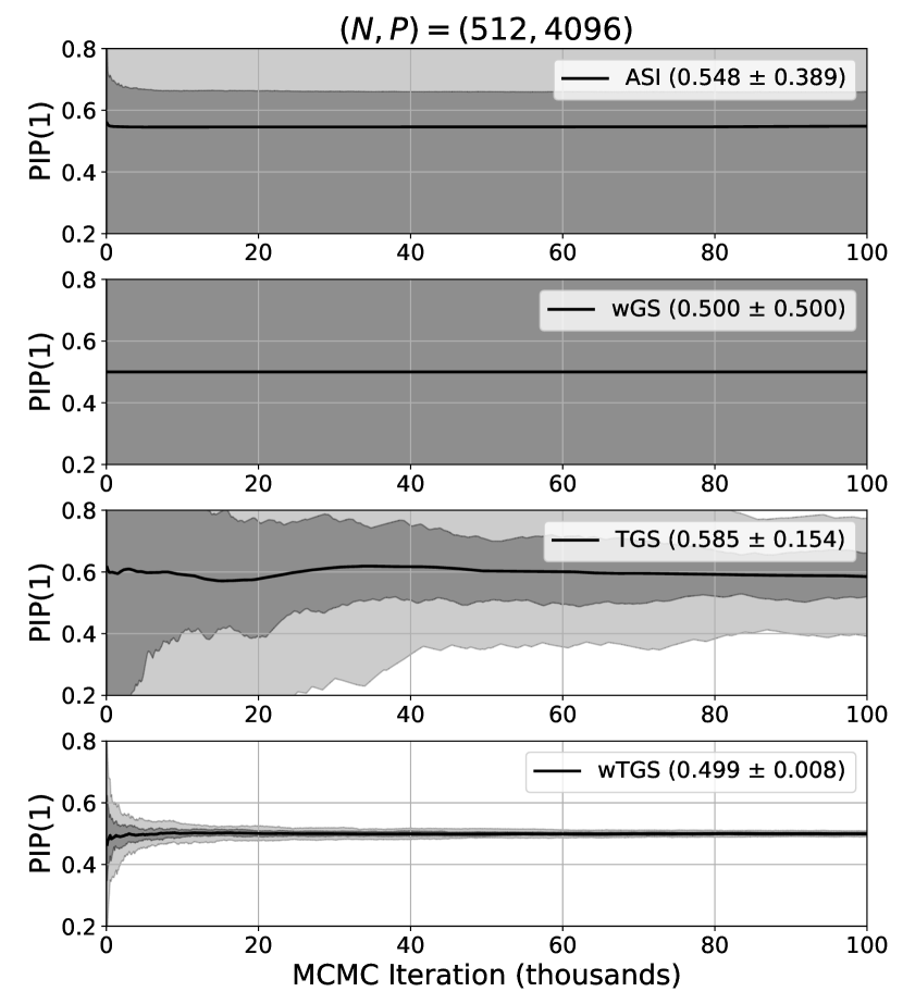
Figure 7: This is a companion figure to Fig. 2. We depict posterior inclusion probability (PIP) estimates for the first covariate in the scenario described in Sec. 5.2 for four different MCMC methods. On the left we depict results for a dataset with $(N,P)=(512,1024)$, while on the right we depict results for a dataset with $(N,P)=(512,4096)$. At each iteration $t$ the PIP is computed using all samples obtained through iteration $t$. The mean PIP is depicted with a solid black line and light and dark grey confidence intervals denote $10\%\!-\!90\%$ and $30\%\!-\!70\%$ quantiles, respectively. The true PIP is almost exactly $\tfrac{1}{2}$. In each case we run 100 independent chains. For each method we also report the final PIP estimate (mean and standard deviation) in parentheses.

Gene	wTGS-5M	wTGS-250k	ASI-250k
DUSP4	1.000	1.000 / 1.000	1.000 / 1.000
PPP2R3A	0.669	0.576 / 0.647	0.466 / 0.318
MIA	0.383	0.338 / 0.365	0.282 / 0.138
KRT80	0.272	0.364 / 0.296	0.502 / 0.482
RELN	0.243	0.286 / 0.219	0.346 / 0.502
ZNF132	0.096	0.124 / 0.093	0.120 / 0.142
TRIM51	0.094	0.075 / 0.099	0.080 / 0.053
ZNF471	0.083	0.107 / 0.081	0.139 / 0.181
S100B	0.063	0.053 / 0.068	0.028 / 0.022
ZNF571	0.062	0.065 / 0.058	0.064 / 0.065
ZNF304	0.060	0.067 / 0.069	0.095 / 0.068
ZNF772	0.040	0.039 / 0.034	0.044 / 0.028
RXRG	0.032	0.026 / 0.025	0.010 / 0.028
ZNF17	0.031	0.033 / 0.037	0.047 / 0.040
ZNF134	0.026	0.026 / 0.029	0.026 / 0.033
KRT7	0.025	0.025 / 0.021	0.016 / 0.206
ZNF71	0.020	0.022 / 0.014	0.045 / 0.023
CCIN	0.019	0.035 / 0.037	0.019 / 0.026
ZNF419	0.018	0.019 / 0.017	0.018 / 0.006
ZMYM3	0.017	0.016 / 0.027	0.014 / 0.036

Gene	wTGS-5M	wTGS-250k	ASI-250k
HNF1B	1.000	1.000 / 1.000	1.000 / 1.000
CAP2	0.323	0.322 / 0.354	0.079 / 0.068
C12orf54	0.172	0.113 / 0.152	0.145 / 0.005
AQP1	0.122	0.127 / 0.128	0.061 / 0.096
FAM43B	0.067	0.059 / 0.050	0.013 / 0.077
KLRF1	0.063	0.059 / 0.065	0.032 / 0.034
ARMC4	0.059	0.062 / 0.035	0.027 / 0.120
SERPINE1	0.050	0.047 / 0.052	0.040 / 0.003
CLIC6	0.049	0.050 / 0.057	0.013 / 0.094
GSDME	0.048	0.056 / 0.050	0.101 / 0.066
UGCG	0.044	0.042 / 0.034	0.108 / 0.093
NEK6	0.039	0.041 / 0.041	0.019 / 0.005
SERPINA10	0.032	0.027 / 0.026	0.007 / 0.017
ECH1	0.029	0.028 / 0.022	0.054 / 0.029
KIF1C	0.029	0.034 / 0.024	0.066 / 0.081
S100A4	0.028	0.029 / 0.025	0.083 / 0.009
MSANTD3	0.023	0.029 / 0.023	0.005 / 0.006
PLIN3	0.023	0.019 / 0.020	0.043 / 0.007
IL4R	0.021	0.018 / 0.021	0.016 / 0.003
SHBG	0.020	0.016 / 0.022	0.005 / 0.027

Table 1: These tables are companions to Fig. 4-5. We depict PIP estimates for DUSP4 (left) and HNF1B (right). In each case we include the result from a wTGS run with five million samples as well as two shorter runs from wTGS and ASI. We depict the top 20 genes as determined by the long wTGS run. The much lower variance and higher accuracy of wTGS are apparent.

A.7 Experimental details

Unless specified otherwise we set $\tau=0.01$ and $h=5/P$ throughout our experiments.

wGS/TGS/wTGS

We choose the exploration parameter $\epsilon$ to be $\epsilon=5$ (see Eqn. 15). We use the $\xi$-adaptation scheme described in Sec. A.4.

ASI

ASI has several hyperparameters which we set as follows. We set the exponent $\lambda_{\rm ASI}$ that controls adaptation to $\lambda_{\rm ASI}=0.75$. We set $\epsilon_{\rm ASI}=0.1/P$ as suggested by the authors. We target an acceptance probability of $\tau_{\rm ASI}=0.25$.

Runtime experiment

For each value of $N$ and $P$ we run each MCMC chain for 2000 burn-in iterations and report iteration times averaged over a subsequent $10^{4}$ iterations.

Correlated covariates scenario

The covariates for $p=3,4,...,P$ are generated independently from a standard Normal distribution: $X_{n,p}\sim\mathcal{N}(0,1)$ for all $n$. We then generate $z\in\mathbb{R}^{N}$ with $z_{n}\sim\mathcal{N}(0,1)$ and set $X_{n,p=1}\sim\mathcal{N}(z_{n},10^{-4})$ and $X_{n,p=2}\sim\mathcal{N}(z_{n},10^{-4})$. That is the first two covariates are almost identical apart from a small amount of noise. We then generate the responses $Y_{n}$ using success logits given by $\psi_{n}=z_{n}$. The total count $C_{n}$ for each data point is set to 10. Consequently the true posterior concentrates on two modes with $\gamma=(1,0,0,...)$ and $\gamma=(0,1,0,...)$. We set $h=1/P$ and run each algorithm for 10 thousand burn-in/warmup iterations and use the subsequent 100 thousand samples for analysis.

Cancer data

All chains are run for 25 thousand burn-in/warmup iterations.

Hospital data

We run wTGS for 10 thousand burn-in iterations and use the subsequent 100 thousand samples for analysis. The $899$ held-out patients are chosen at random. We use a random walk proposal scale for $\log\nu$ of $0.03$. We set $\psi_{0}$ to be the logarithm of the mean of the observed $Y$ (this is equivalent to shifting the prior mean of the bias $\beta_{0}$; see Sec A.5).

Health survey data

We run wTGS for 10 thousand burn-in iterations and use the subsequent 100 thousand samples for analysis. We use a random walk proposal scale for $\log\nu$ of $0.03$. We set $\psi_{0}$ to be the logarithm of the mean of the observed $Y$ (this is equivalent to shifting the prior mean of the bias $\beta_{0}$; see Sec A.5).

References

- Behan et al. [2019] Fiona M Behan, Francesco Iorio, Gabriele Picco, Emanuel Gonçalves, Charlotte M Beaver, Giorgia Migliardi, Rita Santos, Yanhua Rao, Francesco Sassi, Marika Pinnelli, et al. Prioritization of cancer therapeutic targets using crispr–cas9 screens. Nature, 568(7753):511–516, 2019.
- Bleki [2021] Zolisa Bleki. polyagamma: An efficient and flexible sampler of the polya-gamma distribution with a numpy/scipy compatible interface., May 2021. URL https://pypi.org/project/polyagamma/.
- Chipman et al. [2001] Hugh Chipman, Edward I George, Robert E McCulloch, Merlise Clyde, Dean P Foster, and Robert A Stine. The practical implementation of bayesian model selection. Lecture Notes-Monograph Series, pages 65–134, 2001.
- Dawid [1984] A Philip Dawid. Present position and potential developments: Some personal views statistical theory the prequential approach. Journal of the Royal Statistical Society: Series A (General), 147(2):278–290, 1984.
- Dellaportas et al. [2002] Petros Dellaportas, Jonathan J Forster, and Ioannis Ntzoufras. On bayesian model and variable selection using mcmc. Statistics and Computing, 12(1):27–36, 2002.
- DepMap [2019a] DepMap. Wellcome sanger institute. cancer dependency map., 2019a. URL https://depmap.sanger.ac.uk/.
- DepMap [2019b] DepMap. Broad institute of harvard and mit. cancer dependency map., 2019b. URL https://depmap.org/.
- Garcia-Donato and Martinez-Beneito [2013] Gonzalo Garcia-Donato and Miguel A Martinez-Beneito. On sampling strategies in bayesian variable selection problems with large model spaces. Journal of the American Statistical Association, 108(501):340–352, 2013.
- George and McCulloch [1993] Edward I George and Robert E McCulloch. Variable selection via gibbs sampling. Journal of the American Statistical Association, 88(423):881–889, 1993.
- George and McCulloch [1997] Edward I George and Robert E McCulloch. Approaches for bayesian variable selection. Statistica sinica, pages 339–373, 1997.
- Griffin et al. [2021] JE Griffin, KG Łatuszyński, and MFJ Steel. In search of lost mixing time: adaptive markov chain monte carlo schemes for bayesian variable selection with very large p. Biometrika, 108(1):53–69, 2021.
- Hilbe and Greene [2007] JM Hilbe and WH Greene. Count response regression models, in (eds) cr rao, jp miller, and dc rao, epidemiology and medical statistics, 2007.
- Hilbe [2011] Joseph M Hilbe. Negative binomial regression. Cambridge University Press, 2011.
- Lamnisos et al. [2009] Demetris Lamnisos, Jim E Griffin, and Mark FJ Steel. Transdimensional sampling algorithms for bayesian variable selection in classification problems with many more variables than observations. Journal of Computational and Graphical Statistics, 18(3):592–612, 2009.
- Liu [1996] Jun S Liu. Peskun’s theorem and a modified discrete-state gibbs sampler. Biometrika, 83(3), 1996.
- McCullagh and Nelder [2019] Peter McCullagh and John A Nelder. Generalized linear models. Routledge, 2019.
- Meyers et al. [2017] Robin M Meyers, Jordan G Bryan, James M McFarland, Barbara A Weir, Ann E Sizemore, Han Xu, Neekesh V Dharia, Phillip G Montgomery, Glenn S Cowley, Sasha Pantel, et al. Computational correction of copy number effect improves specificity of crispr–cas9 essentiality screens in cancer cells. Nature genetics, 49(12):1779–1784, 2017.
- Nikooienejad et al. [2016] Amir Nikooienejad, Wenyi Wang, and Valen E Johnson. Bayesian variable selection for binary outcomes in high-dimensional genomic studies using non-local priors. Bioinformatics, 32(9):1338–1345, 2016.
- O’Hara et al. [2009] Robert B O’Hara, Mikko J Sillanpää, et al. A review of bayesian variable selection methods: what, how and which. Bayesian analysis, 4(1):85–117, 2009.
- Pacini et al. [2021] Clare Pacini, Joshua M Dempster, Isabella Boyle, Emanuel Gonçalves, Hanna Najgebauer, Emre Karakoc, Dieudonne van der Meer, Andrew Barthorpe, Howard Lightfoot, Patricia Jaaks, et al. Integrated cross-study datasets of genetic dependencies in cancer. Nature communications, 12(1):1–14, 2021.
- [21] Adam Paszke, Sam Gross, Francisco Massa, Adam Lerer, James Bradbury, Gregory Chanan, Trevor Killeen, Zeming Lin, Natalia Gimelshein, Luca Antiga, et al. Pytorch: An imperative style, high-performance deep learning library.
- Polson et al. [2013] Nicholas G Polson, James G Scott, and Jesse Windle. Bayesian inference for logistic models using pólya–gamma latent variables. Journal of the American statistical Association, 108(504):1339–1349, 2013.
- Shin et al. [2018] Minsuk Shin, Anirban Bhattacharya, and Valen E Johnson. Scalable bayesian variable selection using nonlocal prior densities in ultrahigh-dimensional settings. Statistica Sinica, 28(2):1053, 2018.
- Steel and Ley [2007] Mark FJ Steel and Eduardo Ley. On the effect of prior assumptions in Bayesian model averaging with applications to growth regression. The World Bank, 2007.
- Tanner and Wong [1987] Martin A Tanner and Wing Hung Wong. The calculation of posterior distributions by data augmentation. Journal of the American statistical Association, 82(398):528–540, 1987.
- Tian et al. [2019] Yiqing Tian, Howard D Bondell, and Alyson Wilson. Bayesian variable selection for logistic regression. Statistical Analysis and Data Mining: The ASA Data Science Journal, 12(5):378–393, 2019.
- Wan and Griffin [2021] Kitty Yuen Yi Wan and Jim E Griffin. An adaptive mcmc method for bayesian variable selection in logistic and accelerated failure time regression models. Statistics and Computing, 31(1):1–11, 2021.
- Zanella and Roberts [2019] Giacomo Zanella and Gareth Roberts. Scalable importance tempering and bayesian variable selection. Journal of the Royal Statistical Society: Series B (Statistical Methodology), 81(3):489–517, 2019.