Hop-Constrained Metric Embeddings and their Applications

Abstract

In network design problems, such as compact routing, the goal is to route packets between nodes using the (approximated) shortest paths. A desirable property of these routes is a small number of hops, which makes them more reliable, and reduces the transmission costs.

Following the overwhelming success of stochastic tree embeddings for algorithmic design, Haeupler, Hershkowitz, and Zuzic (STOC’21) studied hop-constrained Ramsey-type metric embeddings into trees. Specifically, embedding $f:G(V,E)\rightarrow T$ has Ramsey hop-distortion $(t,M,\beta,h)$ (here $t,\beta,h\geq 1$ and $M\subseteq V$) if $\forall u\in M,v\in V$, $d_{G}^{(\beta\cdot h)}(u,v)\leq d_{T}(u,v)\leq t\cdot d_{G}^{(h)}(u,v)$. $t$ is called the distortion, $\beta$ is called the hop-stretch, and $d_{G}^{(h)}(u,v)$ denotes the minimum weight of a $u-v$ path with at most $h$ hops. Haeupler et al. constructed embedding where $M$ contains $1-\epsilon$ fraction of the vertices and $\beta=t=O(\frac{\log^{2}n}{\epsilon})$. They used their embedding to obtain multiple bicriteria approximation algorithms for hop-constrained network design problems.

In this paper, we first improve the Ramsey-type embedding to obtain parameters $t=\beta=\frac{\tilde{O}(\log n)}{\epsilon}$, and generalize it to arbitrary distortion parameter $t$ (in the cost of reducing the size of $M$). This embedding immediately implies polynomial improvements for all the approximation algorithms from Haeupler et al.. Further, we construct hop-constrained clan embeddings (where each vertex has multiple copies), and use them to construct bicriteria approximation algorithms for the group Steiner tree problem, matching the state of the art of the non constrained version. Finally, we use our embedding results to construct hop constrained distance oracles, distance labeling, and most prominently, the first hop constrained compact routing scheme with provable guarantees. All our metric data structures almost match the state of the art parameters of the non-constrained versions.

1 Introduction

Low distortion metric embeddings provide a powerful algorithmic toolkit, with applications ranging from approximation/sublinear/online/distributed algorithms [LLR95, AMS99, BCL⁺18, KKM⁺12] to machine learning [GKK17], biology [HBK⁺03], and vision [AS03]. The basic idea in order to solve a problem in a “hard” metric space $(X,d_{X})$, is to embed the points $X$ into a “simple” metric space $(Y,d_{Y})$ that preserves all pairwise distances up to small multiplicative factor. Then one solve the problem in $Y$, and “pull-back” the solution into $X$.

A highly desirable target space is trees, as many hard problems become easy once the host space is a tree metric. Fakcharoenphol, Rao, and Talwar [FRT04] (improving over [AKPW95, Bar96, Bar98], see also [Bar04]) showed that every $n$ point metric space could be embedded into distribution $\mathcal{D}$ over dominating trees with expected distortion $O(\log n)$. Formally, $\forall x,y\in X$, $T\in\mathrm{supp}(\mathcal{D})$, $d_{X}(x,y)\leq d_{T}(x,y)$, and $\mathbb{E}_{T\sim\mathcal{D}}[d_{T}(x,y)]\leq O(\log n)\cdot d_{X}(x,y)$. This stochastic embedding enjoyed tremendous success and has numerous applications. However, the distortion guarantee is only in expectation. A different solution is Ramsey type embeddings which have a worst case guarantee, however only w.r.t. a subset of the points. Specifically, Mendel and Naor [MN07] (see also [BFM86, BBM06, BLMN05a, NT12, BGS16, ACE⁺20, Bar21]) showed that for every parameter $k$, every $n$-point metric space contains a subset $M$ of at least $n^{1-\frac{1}{k}}$ points, where $X$ could be embedded into a tree such that all the distances in $M\times X$ are preserved up to an $O(k)$ multiplicative factor. Formally, $\forall x,y\in X$, $d_{X}(x,y)\leq d_{T}(x,y)$, and $\forall x\in M,y\in X$, $d_{T}(x,y)\leq O(k)\cdot d_{X}(x,y)$. Finally, in order to obtain worst case guarantee w.r.t. all point pairs, the author and Hung [FL21a] introduced clan embeddings into trees. Here each point $x$ is mapped into a subset $f(x)\subseteq Y$ which called copies of $x$, with a special chief copy $\chi(x)\in f(x)$. For every parameter $k$, [FL21a] constructed distribution over dominating clan embeddings such that for every pair of vertices $x,y$, some copy of $x$ is close to the chief of $y$: $d_{X}(x,y)\leq\min_{x^{\prime}\in f(x),y^{\prime}\in f(y)}d_{T}(x^{\prime},y^{\prime})\leq\min_{x^{\prime}\in f(x)}d_{T}(x^{\prime},\chi(y))\leq O(k)\cdot d_{X}(x,y)$, and the expected number of copies of every vertex is bounded: $\mathbb{E}[|f(x)|]=O(n^{\frac{1}{k}})$.

In many applications, the metric space is the shortest path metric $d_{G}$ of a weighted graph $G=(V,E,w)$. Here, in addition to metric distances, there are often hop-constrains. For instance, one may wish to route a packet between two nodes, using a path with at most ${\color[rgb]{1,0,0}h}$ hops, i.e. the number of edges in the path. Such hop constrains are desirable as each transmission causes delays, which are non-negligible when the number of transmissions is large [AT11, BF18]. Another advantage is that low-hop routes are more reliable: if each transmission is prone to failure with a certain probability, then low-hop routes are much more likely to reach their destination [BF18, WA88, RAJ12]. Electricity and telecommunications distribution network configuration problems include hop constraints that limit the maximum number of edges between a customer and its feeder [BF18], and there are many other (practical) network design problems with hop constraints [LCM99, BA92, GPdSV03, GM03, PS03]. Hop-constrained network approximation is often used in parallel computing [Coh00, ASZ20], as the number of hops governs the number of required parallel rounds (e.g. in Dijkstra). Finally, there is an extensive work on approximation algorithms for connectivity problems like spanning tree and Steiner tree with hop constraints [Rav94, KP97, MRS⁺98, AFH⁺05, KLS05, KP09, HKS09, KS16], and for some generalizations in [HHZ21b].

Given a weighted graph $G=(V,E,w)$, $d_{G}^{{\color[rgb]{1,0,0}(h)}}(u,v)$ denotes the minimum weight of a $u$-$v$ path containing at most ${\color[rgb]{1,0,0}h}$ hops. Following the tremendous success of tree embeddings, Haeupler, Hershkowitz and Zuzic [HHZ21b] suggested to study hop-constrained tree embeddings. That is, embedding the vertex set $V$ into a tree $T$, such that $d_{T}(u,v)$ will approximate the ${\color[rgb]{1,0,0}h}$-hop constrained distance $d_{G}^{{\color[rgb]{1,0,0}(h)}}(u,v)$. Unfortunately, [HHZ21b] showed that $d_{G}^{{\color[rgb]{1,0,0}(h)}}$ is very far from being a metric space, and the distortion of every embedding of $d_{G}^{{\color[rgb]{1,0,0}(h)}}$ is unbounded. To overcome this issue, [HHZ21b] allowed hop-stretch. Specifically, allowing bi-criteria approximation in the following sense: $d_{G}^{{\color[rgb]{1,0,0}(\beta\cdot h)}}(u,v)\leq d_{T}(u,v)\leq t\cdot d^{{\color[rgb]{1,0,0}(h)}}_{G}(u,v)$, for some parameters ${\color[rgb]{1,0,0}\beta}$, and $t$. However, even this relaxation is not enough as long as ${\color[rgb]{1,0,0}\beta\cdot h}<n-1$. To see this, consider the unweighted $n$-path $P_{n}=\{v_{0},\dots,v_{n-1}\}$. Then $d_{G}^{{\color[rgb]{1,0,0}(n-2)}}(v_{0},v_{n-1})=\infty$, implying that for every metric $X$ over $V$, $\max_{i}\{d_{X}(v_{i},v_{i+1})\}\geq\frac{1}{n-1}\sum_{i}d_{X}(v_{i},v_{i+1})\geq\frac{d_{X}(v_{0},v_{n-1})}{n-1}\geq\frac{d_{G}^{{\color[rgb]{1,0,0}(n-2)}}(v_{0},v_{n-1})}{n-1}=\infty$. As a result, some pairs have distortion $\infty$, and hence no bi-criteria metric embedding is possible. In particular, there is no hop-constrained counterpart for [FRT04].

To overcome this barrier, [HHZ21b] studied hop-constrained Ramsey-type tree embeddings. Their main result, is that every $n$-point weighted graph $G=(V,E,w)$ with polynomial aspect ratio, and parameter $\epsilon\in(0,1)$, there is distribution over pairs $(T,M)$, where $M\subseteq V$, and $T$ is a tree with $M$ as its vertex set such that

$$\forall u,v\in M,\qquad d_{G}^{{\color[rgb]{1,0,0}(O(\frac{\log^{2}n}{\epsilon})\cdot h)}}(u,v)\leq d_{T}(u,v)\leq O(\frac{\log^{2}n}{\epsilon})\cdot d_{G}^{{\color[rgb]{1,0,0}(h)}}(u,v)\leavevmode\nobreak\ ,$$

and for every $v\in V$, $\Pr[v\in M]\geq 1-\epsilon$ (referred to as inclusion probability). Improving the distortion, and hop-stretch, was left as the “main open question” in [HHZ21b].

Question 1 ([HHZ21b]).

Is it possible to construct better hop-constrained Ramsey-type tree embeddings? What are the optimal parameters?

Adding hop-constrains to a problem often makes it considerably harder. For example, obtaining $o(\log n)$ approximation for the Hop constrained MST problem (where the hop-diameter must be bounded by ${\color[rgb]{1,0,0}h}$) is NP-hard [BKP01], while MST is simple problem without it. Similarly, for every ${\epsilon>0}$, obtaining $o(2^{\log^{1-\epsilon}}n)$-approximation for the hop-constrained Steiner forest problem is NP-hard [DKR16] (while constant approximation is possible without hop constrains [AKR95]).

[HHZ21b] used their hop-constrained Ramsey-type tree embeddings to construct many approximation algorithms. Roughly, given that some problem has (non constrained) approximation ratio $\alpha$ for trees, [HHZ21b] obtain a bicriteria approximation for the hop constrained problem with cost $O(\alpha\cdot\log^{3}n)$, and hop-stretch $O(\log^{3}n)$. For example, in the group Steiner tree problem we are given $k$ sets $g_{1},\dots,g_{k}\subseteq V$, and a root vertex $r\in V$. The goal is to construct a minimal weight tree spanning the vertex $r$ and at least one vertex from each group (set) $g_{i}$. In the hop-constrained version of the problem, we are given in addition a hop-bound ${\color[rgb]{1,0,0}h}$, and the requirement is to find a minimum weight subgraph $H$, such that for every $g_{i}$, $\mathrm{hop}_{H}(r,g_{i})\leq{\color[rgb]{1,0,0}h}$. Denote by $\mathrm{OPT}$ the weight of the optimal solution. In the non-constrained version, where the input metric is a tree, [GKR00] provided a $O(\log n\cdot\log k)$ approximation. Using the scheme of [HHZ21b], one can find a solution $H$ of weight $O(\log^{4}n\cdot\log k)\cdot\mathrm{OPT}$, such that for every $g_{i}$, $\mathrm{hop}_{H}(r,g_{i})\leq{\color[rgb]{1,0,0}O(\log^{3}n)\cdot h}$. The best approximation for the non-constrained group Steiner tree problem is $O(\log^{2}n\cdot\log k)$ [GKR00]. Clearly, every improvement over the hop-constrained Ramsey-type embedding will imply better bicriteria approximation algorithms. However, even if one would use [HHZ21b] framework on optimal Ramsey-type embeddings (ignoring hop-constrains), the cost factors will be inferior compared to the non-constrained versions (specifically $O(\log^{3}n\cdot\log k)$ for GST). It is interesting to understand whether there is a separation between the cost of a bicriteria approximation for hop-constrained problems to their non-constrained counterparts. A more specific question is the following:

Question 2.

Could one match the state of the art cost approximation of the (non hop-constrained) group Steiner tree problem while having $\mathrm{polylog}(n)$ hop-stretch?

Metric data structures such as distance oracles, distance labeling, and compact routing schemes are extensively studied, and widely used throughout algorithmic design. A natural question is whether one can construct similar data structures w.r.t. hop-constrained distances. Most prominently is the question of compact routing scheme [TZ01], where one assigns each node in a network a short label and small local routing table, such that packets could be routed throughout the network with routes not much longer than the shortest paths. Hop-constrained routing is a natural question due to it’s clear advantages (bounding transmission delays, and increasing reliability). Indeed, numerous papers developed different heuristics for different models of hop-constrained routing. However, to the best knowledge of the author, no prior provable guarantees were provided for hop-constrained compact routing scheme.

Question 3.

What hop-constrained compact routing schemes are possible?

1.1 Our contribution

1.1.1 Metric embeddings

Here we present our metric embedding results. Our embeddings will be into ultrametrics, which are structured type of trees having the strong triangle inequality (see Definition 1). Our first contribution is an improved Ramsey-type hop-constrained embedding into trees, partially solving 1. Embedding $f:V(G)\rightarrow U$ is said to have Ramsey hop-distortion $(t,M,{\color[rgb]{1,0,0}\beta},{\color[rgb]{1,0,0}h})$ if $\forall u,v\in V$ $d_{G}^{{\color[rgb]{1,0,0}(\beta\cdot h)}}(u,v)\leq d_{U}(u,v)$, and $\forall u\in M,v\in V$, $d_{U}(u,v)\leq t\cdot d_{G}^{{\color[rgb]{1,0,0}(h)}}(u,v)$ (see Definition 4).

Theorem 1 (Hop Constrained Ramsey Embedding).

Consider an $n$-vertex graph $G=(V,E,w)$ with polynomial aspect ratio, and parameters $k,{\color[rgb]{1,0,0}h}\in[n]$. Then there is a distribution $\mathcal{D}$ over dominating ultrametrics, such that:

1. Every $U\in\mathrm{supp}(\mathcal{D})$, has Ramsey hop-distortion $(O(k),M,{\color[rgb]{1,0,0}O(k\cdot\log n)},{\color[rgb]{1,0,0}h})$, where $M\subseteq V$ is a random variable.

2. For every $v\in V$, $\Pr_{U\sim\mathcal{D}}[v\in M]\geq\Omega(n^{-\frac{1}{k}})$.

In addition, for every $\epsilon\in(0,1)$, there is distribution $\mathcal{D}$ as above such that every $U\in\mathrm{supp}(\mathcal{D})$ has Ramsey hop-distortion $(O(\frac{\log n}{\epsilon}),M,{\color[rgb]{1,0,0}O(\frac{\log^{2}n}{\epsilon})},{\color[rgb]{1,0,0}h})$, and for every $v\in V$, $\Pr[v\in M]\geq 1-\epsilon$.

Ignoring the hop-distortion (e.g. setting ${\color[rgb]{1,0,0}h=n}$), the tradeoff in Theorem 1 between the distortion to the inclusion probability is asymptotically tight (see [BBM06, FL21a]). However, it is yet unclear what is the best possible hop-stretch obtainable with asymptotically optimal distortion-inclusion probability tradeoff. Interestingly, we show that by increasing the distortion by a $\log\log n$ factor, one can obtain sub-logarithmic hop-stretch. Further, in this version we can also drop the polynomial aspect ratio assumption.

Theorem 2 (Hop Constrained Ramsey Embedding).

Consider an $n$-vertex graph $G=(V,E,w)$, and parameters $k,{\color[rgb]{1,0,0}h}\in[n]$. Then there is a distribution $\mathcal{D}$ over dominating ultrametrics with $V$ as leafs, such that every $U\in\mathrm{supp}(\mathcal{D})$ has Ramsey hop-distortion $(O(k\cdot\log\log n),M,{\color[rgb]{1,0,0}O(k\cdot\log\log n)},{\color[rgb]{1,0,0}h})$, where $M\subseteq V$ is a random variable, and $\forall v\in V$, $\Pr_{U\sim\mathcal{D}}[v\in M_{U}]\geq\Omega(n^{-\frac{1}{k}})$
In addition, for every $\epsilon\in(0,1)$, there is distribution $\mathcal{D}$ as above such that every $U\in\mathrm{supp}(\mathcal{D})$ has Ramsey hop-distortion $(O(\frac{\log n\cdot\log\log n}{\epsilon}),M,{\color[rgb]{1,0,0}O(\frac{\log n\cdot\log\log n}{\epsilon})},{\color[rgb]{1,0,0}h})$, and $\forall v\in V$, $\Pr[v\in M]\geq 1-\epsilon$.

Next, we construct hop-constrained clan embedding $(f,\chi)$. Embedding $f:V(G)\rightarrow 2^{U}$ is said to have hop-distortion $(t,{\color[rgb]{1,0,0}\beta},{\color[rgb]{1,0,0}h})$ if $\forall u,v\in V$, $d^{{\color[rgb]{1,0,0}(\beta\cdot h)}}_{G}(x,y)\leq\min_{u^{\prime}\in f(u),v^{\prime}\in f(v)}d_{U}(u^{\prime},v^{\prime})\leq\min_{u^{\prime}\in f(u)}d_{U}(u^{\prime},\chi(v))\leq t\cdot d^{{\color[rgb]{1,0,0}(h)}}_{G}(u,v)$. See Definition 3 for formal definition, and Definition 7 of hop-path-distortion.

Theorem 3 (Clan embedding into ultrametric).

Consider an $n$-vertex graph $G=(V,E,w)$ with polynomial aspect ratio, and parameters $k,{\color[rgb]{1,0,0}h}\in[n]$. Then there is a distribution $\mathcal{D}$ over clan embeddings $(f,\chi)$ into ultrametrics with hop-distortion $\left(O(k),{\color[rgb]{1,0,0}O(k\cdot\log n)},{\color[rgb]{1,0,0}h}\right)$, hop-path-distortion $\left({O(k\cdot\log n)},{\color[rgb]{1,0,0}h}\right)$, and such that for every vertex $v\in V$, $\mathbb{E}_{f\sim\mathcal{D}}[|f(v)|]\leq O(n^{\frac{1}{k}})$.

In addition, for every $\epsilon\in(0,1)$, there is distribution $\mathcal{D}$ as above such that every $U\in\mathrm{supp}(\mathcal{D})$ has hop-distortion $\left(O(\frac{\log n}{\epsilon}),{\color[rgb]{1,0,0}O(\frac{\log^{2}n}{\epsilon})},{\color[rgb]{1,0,0}h}\right)$, hop-path-distortion $\left({O(\frac{\log^{2}n}{\epsilon})},{\color[rgb]{1,0,0}h}\right)$, and such that for every vertex $v\in V$, $\mathbb{E}_{f\sim\mathcal{D}}[|f(v)|]\leq 1+\epsilon$.

Similarly to the Ramsey case, the tradeoff in Theorem 3 between the distortion to the expected clan size is asymptotically optimal [FL21a]. However, it is yet unclear what is the best possible hop-stretch obtainable with asymptotically optimal distortion-expected clan size tradeoff. Here as well we show that by increasing the distortion by a $\log\log n$ factor, one can obtain sub-logarithmic hop-stretch. The polynomial aspect ratio assumption is dropped as well.

Theorem 4 (Clan embedding into ultrametric).

Consider an $n$-vertex graph $G=(V,E,w)$, and parameters $k,{\color[rgb]{1,0,0}h}\in[n]$. Then there is a distribution $\mathcal{D}$ over clan embeddings $(f,\chi)$ into ultrametrics with hop-distortion $\left(O(k\cdot\log\log n),{\color[rgb]{1,0,0}O(k\cdot\log\log n)},{\color[rgb]{1,0,0}h}\right)$, hop-path-distortion $\left(O(k\cdot\log n\cdot\log\log n),{\color[rgb]{1,0,0}h}\right)$, and such that for every point $v\in V$, $\mathbb{E}_{f\sim\mathcal{D}}[|f(v)|]\leq O(n^{\frac{1}{k}})$.

In addition, for every $\epsilon\in(0,1)$, there is distribution $\mathcal{D}$ as above such that every $U\in\mathrm{supp}(\mathcal{D})$ has hop-distortion $\left(O(\frac{\log n\cdot\log\log n}{\epsilon}),{\color[rgb]{1,0,0}O(\frac{\log n\cdot\log\log n}{\epsilon})},{\color[rgb]{1,0,0}h}\right)$, hop-path-distortion $\left({O(\frac{\log^{2}n\cdot\log\log n}{\epsilon})},{\color[rgb]{1,0,0}h}\right)$, and such that for every vertex $v\in V$, $\mathbb{E}_{f\sim\mathcal{D}}[|f(v)|]\leq 1+\epsilon$.

Our final embedding result is a one-to-many “subgraph preserving” embedding. A path-tree one-to-many embedding $f$ is a map where each path $P$ in $T$ between copies $u^{\prime}\in f(u),v^{\prime}\in f(v)$ is associated with a path in $G$ from $u$ to $v$. Such an embedding is said to have hop bound ${\color[rgb]{1,0,0}\beta}$ if every such associated path in $G$ has at most ${\color[rgb]{1,0,0}\beta}$ hops (see Definition 8).

Theorem 5 (Subgraph Preserving Embedding).

Consider an $n$-point graph $G=(V,E,w)$ with polynomial aspect ratio, parameter ${\color[rgb]{1,0,0}h}\in\mathbb{N}$ and vertex $r\in V$. Then there is a path-tree one-to-many embedding $f$ of $G$ into a tree $T$ with hop bound ${\color[rgb]{1,0,0}O(\log^{3}n)\cdot h}$, $|f(V)|=O(n^{1.5})$, $|f(r)|=1$, and such that for every sub-graph $H$, there is a subgraph $H^{\prime}$ of $T$ where for every $u,v\in H$ with $\mathrm{hop}_{H}(u,v)\leq{\color[rgb]{1,0,0}h}$, $H^{\prime}$ contains a pair of copies $u^{\prime}\in f(u)$ and $v^{\prime}\in f(v)$ in the same connected component. Further, $w_{T}(H^{\prime})\leq O(\log n)\cdot w(H)$.

In Theorem 11 we prove an alternative version of Theorem 5 where the hop bound is ${\color[rgb]{1,0,0}\tilde{O}(\log^{2}n)\cdot h}$ and the bound on the weight of $H^{\prime}$ is only $\tilde{O}(\log n)\cdot w(H)$. [HHZ21b] obtained a theorem similar to Theorem 5, where they have the same hop bound, and the differences are that $|f(V)|$ is bounded by $\tilde{O}(n)$, and the weight of $H^{\prime}$ is only bounded by $O(\log^{3}n)\cdot w(H)$. Thus we get a cubic improvement.

1.1.2 Approximation algorithms

Hop-Constrained Problem	Cost Apx.	Hop Apx.	Reference
Application of the clan embedding
H.C. Group Steiner Tree	$O(\log^{4}n\cdot\log k)$	$O(\log^{3}n)$	[HHZ21b]
	$O(\log^{2}n\cdot\log k)$	$O(\log^{2}n)$	Theorem 6 (✓)
	$\tilde{O}(\log^{2}n\cdot\log k)$	$\tilde{O}(\log n)$	Theorem 6
H.C. Online Group Steiner Tree	$O(\log^{5}n\cdot\log k)$	$O(\log^{3}n)$	[HHZ21b]
	$O(\log^{3}n\cdot\log k)$	$O(\log^{2}n)$	Theorem 13 (✓)
	$\tilde{O}(\log^{3}n\cdot\log k)$	$\tilde{O}(\log n)$	Theorem 13
H.C. Group Steiner Forest	$O(\log^{6}n\cdot\log k)$	$O(\log^{3}n)$	[HHZ21b]
	$O(\log^{4}n\cdot\log k)$	$O(\log^{3}n)$	Theorem 7
	$\tilde{O}(\log^{4}n\cdot\log k)$	$\tilde{O}(\log^{2}n)$
H.C. Online Group Steiner Forest	$O(\log^{7}n\cdot\log k)$	$O(\log^{3}n)$	[HHZ21b]
	$O(\log^{5}n\cdot\log k)$	$O(\log^{3}n)$	Theorem 14 (✓)
	$\tilde{O}(\log^{5}n\cdot\log k)$	$\tilde{O}(\log^{2}n)$	Theorem 14
Application of the Ramsey type embedding
H.C. Relaxed $k$-Steiner Tree	$O(\log^{3}n)$	$O(\log n)$	[HKS09]
	$O(\log^{2}n)$	$O(\log^{3}n)$	[HHZ21b]
	$O(\log n)$	$O(\log^{3}n)$	Corollary 3
	$\tilde{O}(\log n)$	$\tilde{O}(\log^{2}n)$
H.C. $k$-Steiner Tree	$O(\log^{3}n\cdot\log k)$	$O(\log^{2}n)$	[HKS09]
	$O(\log^{2}n)$	$O(\log n)$	[KS16]
	$O(\log^{2}n\cdot\log k)$	$O(\log^{3}n)$	[HHZ21b]
	$O(\log n\cdot\log k)$	$O(\log^{3}n)$	Corollary 3
	$\tilde{O}(\log n\cdot\log k)$	$\tilde{O}(\log^{2}n)$
H.C. Oblivious Steiner Forest	$O(\log^{3}n)$	$O(\log^{3}n)$	[HHZ21b]
	$O(\log^{2}n)$	$O(\log^{3}n)$	Corollary 3
	$\tilde{O}(\log^{2}n)$	$\tilde{O}(\log^{2}n)$
H.C. Oblivious Network Design	$O(\log^{4}n)$	$O(\log^{3}n)$	[HHZ21b]
	$O(\log^{3}n)$	$O(\log^{3}n)$	Corollary 3
	$\tilde{O}(\log^{3}n)$	$\tilde{O}(\log^{2}n)$

Table 1: Our bicriteria approximation results. All approximation guarantees are in worst case, other than for the two online problems where the approximation is in expectation. All input graphs are assumed to have polynomial (in $n$) aspect ratio. The parameter $k$ in online group Steiner tree/forest, denotes the size of an initial set $\mathcal{K}$ containing all potential requests.
Our results for the group Steiner tree/forest, and online group Steiner tree/forest are based on our hop-constrained clan embedding. All the other results are application of our Ramsey type hop-constrained embedding, and obtained from [HHZ21b] in a black box manner. The results marked with $(\checkmark)$ match the state of the art approximation factor (when one ignores hop constrains). Note that we obtain first improvement over the cost approximation to the well studied h.c. $k$-Steiner tree problems (since the 2011 conference version of [KS16].)

[HHZ21b] used their Ramsey type embeddings to obtain many different approximation algorithms on hop-constrained (abbreviated h.c.). Our improved Ramsey embeddings imply directly improved approximation factors, and hop-stretch, for all these problems. Most prominently, we improve the cost approximation for the well studied h.c. $k$-Steiner tree problem over [KS16] ([KS16] approximation is superior to [HHZ21b]). See Corollary 3 and Table 1 for a summary.

We go beyond applying our embeddings into [HHZ21b] as a black box and obtain further improvements. A subgraph $H$ of $G$ is ${\color[rgb]{1,0,0}h}$-respecting if for every $u,v\in V(H)$, $d^{{\color[rgb]{1,0,0}(h)}}_{G}(u,v)\leq d_{H}(u,v)$. In Corollary 1 we show that there is a one-to-many embedding $f:V(G)\rightarrow 2^{T}$ into a tree, such that for every connected ${\color[rgb]{1,0,0}h}$-respecting subgraph $H$, there is a connected subgraph $H^{\prime}$ of $T$ of weight $O(\log n)\cdot w(H)$ and hop diameter ${\color[rgb]{1,0,0}O(\log^{2}n)\cdot h}$ containing at least one vertex from $f(u)$ for every $u\in V(H)$, see Corollary 1 (alternatively, in Corollary 2 we are guaranteed a similar subgraph of weight $\tilde{O}(\log n)\cdot w(H)$ and hop diameter ${\color[rgb]{1,0,0}\tilde{O}(\log n)\cdot h}$). We use Corollary 1 to construct bicriteria approximation algorithm for the h.c. group Steiner tree problem, the cost of which matches the state of the art for the (non h.c.) group Steiner tree problem, thus answering 2. Later, we apply Corollary 1 on the online h.c. group Steiner tree problem, and obtain competitive ratio that matches the competitive ratio non constrained version (see Theorem 13).

Theorem 6.

Given an instance of the ${\color[rgb]{1,0,0}h}$-h.c. group Steiner tree problem with $k$ groups on a graph with polynomial aspect ratio, there is a poly-time algorithm that returns a subgraph $H$ such that $w(H)\leq O(\log^{2}n\cdot\log k)\cdot\mathrm{OPT}$, and $\mathrm{hop}_{H}(r,g_{i})\leq{\color[rgb]{1,0,0}O(\log^{2}n)\cdot h}$ for every $g_{i}$, where $\mathrm{OPT}$ denotes the weight of the optimal solution.  Alternatively, one can return a subgraph $H$ such that $w(H)\leq\tilde{O}(\log^{2}n\cdot\log k)\cdot\mathrm{OPT}$, and $\mathrm{hop}_{H}(r,g_{i})\leq{\color[rgb]{1,0,0}\tilde{O}(\log n)\cdot h}$ for every $g_{i}$.

Next we study the group h.c. group Steiner forest problem, where we are given parameter ${\color[rgb]{1,0,0}h}$, and $k$ subset pairs $(S_{1},R_{1}),\dots,(S_{k},R_{k})\subseteq V$, where for every $i\in[k]$, $S_{i},R_{i}\subseteq V$. The goal is to construct a minimal weight forest $F$, such that for every $i$, there is a path with at most ${\color[rgb]{1,0,0}h}$ hops from a vertex in $S_{i}$ to a vertex in $R_{i}$. As the optimal solution to the h.c. group Steiner forest is not necessarily ${\color[rgb]{1,0,0}h}$ respecting, we cannot use Corollary 1. Instead, we using our subgraph-preserving embeddings (Theorems 5 and 11) to obtain a bicriteria approximation. A similar result for the online h.c. group Steiner forest problem is presented in Theorem 14.

Theorem 7.

Given an instance of the ${\color[rgb]{1,0,0}h}$-hop-constrained group Steiner forest problem with $k$ groups on a graph with polynomial aspect ratio, there is a poly-time algorithm that returns a subgraph $H$ such that $w(H)\leq O(\log^{4}n\cdot\log k)\cdot\mathrm{OPT}$, and $\mathrm{hop}_{H}(S_{i},R_{i})\leq{\color[rgb]{1,0,0}O(\log^{3}n)\cdot h}$ for every $i$, where $\mathrm{OPT}$ denotes the weight of the optimal solution.  Alternatively, one can return a subgraph $H$ such that $w(H)\leq\tilde{O}(\log^{4}n\cdot\log k)\cdot\mathrm{OPT}$, and $\mathrm{hop}_{H}(S_{i},R_{i})\leq{\color[rgb]{1,0,0}\tilde{O}(\log^{2}n)\cdot h}$ for every $i$.

1.1.3 Hop-constrained metric data structures

In metric data structures, our goal is to construct data structure that will store (estimated) metric distances compactly, and answer distance (or routing) queries efficiently. As the distances returned by such data structure, do not have to respect the triangle inequality, one might hope to avoid any hop-stretch. This is impossible in general. Consider a complete graph with edge weights sampled randomly from $\{1,\alpha\}$ for some large $\alpha$. Clearly, from information theoretic considerations, in order to estimate $d_{G}^{{\color[rgb]{1,0,0}(1)}}$ with arbitrarily large distortion (but smaller than $\alpha$), one must use $\Omega(n^{2})$ space. Therefore, in our metric data structures we will allow hop-stretch.

Distance Oracles.

A distance oracle is a succinct data structure $\mathsf{DO}$ that (approximately) answers distance queries. Chechik [Che15] (improving over previous results [TZ05, RTZ05, MN07, Wul13, Che14]) showed that any metric (or graph) with $n$ points has a distance oracle of size $O(n^{1+\frac{1}{k}})$, that can report any distance in $O(1)$ time with stretch at most $2k-1$ (which is asymptotically optimal assuming Erdős girth conjecture [Erd64]). That is on query $u,v$, the answer $\mathsf{DO}(u,v)$ satisfies $d_{G}(u,v)\leq\mathsf{DO}(u,v)\leq(2k-1)\cdot d_{G}(u,v)$.

Here we introduce the study of h.c. distance oracles. That is, given a parameter ${\color[rgb]{1,0,0}h}$, we would to construct a distance oracle that on query $u,v$, will return $d^{{\color[rgb]{1,0,0}(h)}}(u,v)$, or some approximation of it. Our result is the following:

Theorem 8 (Hop constrained Distance Oracle).

For every weighted graph $G=(V,E,w)$ on $n$ vertices with polynomial aspect ratio, and parameters $k\in\mathbb{N}$, $\epsilon\in(0,1)$, ${\color[rgb]{1,0,0}h}\in\mathbb{N}$, there is an efficiently constructible distance oracle $\mathsf{DO}$ of size $O(n^{1+\frac{1}{k}}\cdot\log n)$, that for every distance query $(u,v)$, in $O(1)$ time returns a value $\mathsf{DO}(u,v)$ such that $d_{G}^{{\color[rgb]{1,0,0}(O(\frac{k\cdot\log\log n}{\epsilon})\cdot h)}}(u,v)\leq\mathsf{DO}(u,v)\leq(2k-1)(1+\epsilon)\cdot d_{G}^{{\color[rgb]{1,0,0}(h)}}(u,v)$.

Distance Labeling.

A distance labeling is a distributed version of a distance oracle. Given a graph $G=(V,E,w)$, each vertex $v$ is assigned a label $\ell(v)$, and there is an algorithm $\mathcal{A}$, that given $\ell(u),\ell(v)$ returns a value $\mathcal{A}(\ell(u),\ell(v))$ approximating $d_{G}(u,v)$. In their celebrated work, Thorup and Zwick [TZ05] constructed a distance labeling scheme with labels of $O(n^{\frac{1}{k}}\cdot\log n)$ size ${}^{\ref{foot:wordsize}}$, and such that in $O(k)$ time, $\mathcal{A}(\ell(u),\ell(v))$ approximates $d_{G}(u,v)$ within a $2k-1$ factor. We refer to [FGK20] for further details on distance labeling (see also [Pel00, GPPR04, EFN18]).

Matoušek [Mat96] showed that every metric space $(X,d)$ could be embedded into $\ell_{\infty}$ of dimension $O(n^{\frac{1}{k}}\cdot k\cdot\log n)$ with distortion $2k-1$ (for the case $k=O(\log n)$, [ABN11] later improved the dimension to $O(\log n)$). As was previously observed, this embedding can serve as a labeling scheme (where the label of each vertex will be the representing vector in the embedding). From this point of view, the main contribution of [TZ05] is the small $O(k)$ query time (as the label size/distortion tradeoff is similar).

Here we introduce the study of h.c. labeling schemes, where the goal is to approximate $d^{{\color[rgb]{1,0,0}(h)}}_{G}(u,v)$. Note that $d^{{\color[rgb]{1,0,0}(h)}}_{G}$ is not a metric function, and in particular does not embed into $\ell_{\infty}$ with bounded distortion. Hence there is no trivial labeling scheme which is embedding based. Our contribution is the following:

Theorem 9 (Hop constrained Distance Labeling).

For every weighted graph $G=(V,E,w)$ on $n$ vertices with polynomial aspect ratio, and parameters $k\in\mathbb{N}$, $\epsilon\in(0,1)$, ${\color[rgb]{1,0,0}h}\in\mathbb{N}$, there is an efficient construction of a distance labeling that assigns each node $v$ a label $\ell(v)$ of size $O(n^{\frac{1}{k}}\cdot\log^{2}n)$, and such that there is an algorithm $\mathcal{A}$ that on input $\ell(u),\ell(v)$, in $O(k)$ time returns a value such that $d_{G}^{{\color[rgb]{1,0,0}(O(\frac{k\cdot\log\log n}{\epsilon})\cdot h)}}(v,u)\leq\mathcal{A}(\ell(v),\ell(u))\leq(2k-1)(1+\epsilon)\cdot d_{G}^{{\color[rgb]{1,0,0}(h)}}(v,u)$.

Compact Routing Scheme.

A routing scheme in a network is a mechanism that allows packets to be delivered from any node to any other node. The network is represented as a weighted undirected graph, and each node can forward incoming data by using local information stored at the node, called a routing table, and the (short) packet’s header. The routing scheme has two main phases: in the preprocessing phase, each node is assigned a routing table and a short label; in the routing phase, when a node receives a packet, it should make a local decision, based on its own routing table and the packet’s header (which may contain the label of the destination, or a part of it), of where to send the packet. The stretch of a routing scheme is the worst-case ratio between the length of a path on which a packet is routed to the shortest possible path. For fixed $k$, the state of the art is by Chechik [Che13] (improving previous works [PU89, ABLP90, AP92, Cow01, EGP03, TZ01]) who obtain stretch $3.68k$ while using $O(k\cdot n^{\frac{1}{k}})$ size ${}^{\ref{foot:wordsize}}$ tables and labels of size $O(k\cdot\log n)$. For stretch $\Omega(\log n)$ further improvements were obtained by Abraham et al. [ACE⁺20], and the Author and Le [FL21a].

Here we introduce the study of h.c. routing schemes, where the goal is to route the packet in a short path with small number of hops. Specially, for parameter ${\color[rgb]{1,0,0}h}$, we are interested in a routing scheme that for every $u,v$ will use a route with at most ${\color[rgb]{1,0,0}\beta\cdot h}$ hops, and weight $\leq t\cdot d^{{\color[rgb]{1,0,0}(h)}}_{G}(u,v)$, for some parameters ${\color[rgb]{1,0,0}\beta},t$. If $\mathrm{hop}_{G}(u,v)\geq{\color[rgb]{1,0,0}h}$, the routing scheme is not required to do anything, and any outcome will be accepted. We answer 3 in the following:

Theorem 10 (Hop constrained Compact Routing Scheme).

For every weighted graph $G=(V,E,w)$ on $n$ vertices with polynomial aspect ratio, and parameters $k\in\mathbb{N}$, $\epsilon\in(0,1)$, ${\color[rgb]{1,0,0}h}\in\mathbb{N}$, there is an efficient construction of a compact routing scheme that assigns each node a table of size $O(n^{\frac{1}{k}}\cdot k\cdot\log n)$, label of size $O(k\cdot\log^{2}n)$, and such that routing a packet from $u$ to $v$, will be done using a path $P$ such that $\mathrm{hop}(P)={\color[rgb]{1,0,0}O(\frac{k^{2}\cdot\log\log n}{\epsilon})\cdot h}$, and $w(P)\leq 3.68k\cdot(1+\epsilon)\cdot d_{G}^{{\color[rgb]{1,0,0}(h)}}(u,v)$. ‘

1.2 Related work

Hop-constrained network design problems, and in particular routing, received considerable attention from the operations research community, see [WA88, Gou95, Gou96, Voß99, GR01, GM03, AT11, RAJ12, BFGP13, BHR13, BFG15, TCG15, DGM⁺16, Lei16, BF18, DMMY18] for a sample of papers.

Approximation algorithm for h.c. problems were previously constructed. They are usually considerably harder than their non h.c. counter parts, and often require for bicriteria approximation. Previously studied problems include minimum depth spanning tree [AFH⁺05], degree bounded minimum diameter spanning tree [KLS05], bounded depth Steiner tree [KP97, KP09], h.c. MST [Rav94], Steiner tree [MRS⁺98], and $k$-Steiner tree [HKS09, KS16]. We refer to [HHZ21b] for further details.

Recently, Ghaffari et al. [GHZ21] obtained a hop-constrained $\mathrm{poly}(\log)$ competitive oblivious routing scheme using techniques based on [HHZ21b] hop-constrained Ramsey trees. Notably, even though the $O(\frac{\log n}{\epsilon})$ distortion in Theorem 1 is superior to the $O(\frac{\log^{2}n}{\epsilon})$ distortion in a similar theorem in [HHZ21b], [HHZ21b] showed that the expected distortion in their embedding is only $\tilde{O}(\log\frac{n}{\epsilon})$. This additional property turned out to be important for the oblivious routing application.

Given a graph $G=(V,E,w)$, a hop-set is a set of edges $G^{\prime}$ that when added to $G$, $d_{G\cup G^{\prime}}^{{\color[rgb]{1,0,0}(h)}}$ well approximates $d_{G}$. Formally, an $(t,{\color[rgb]{1,0,0}h})$-hop-set is a set $G^{\prime}$ such that $\forall u,v\in V$, $d_{G}(u,v)\leq d_{G\cup G^{\prime}}^{{\color[rgb]{1,0,0}(h)}}(u,v)\leq t\cdot d_{G}(u,v)$. Most notably, [EN19] constructed $\left(1+\epsilon,{\color[rgb]{1,0,0}\left(\frac{\log k}{\epsilon}\right)^{\log k-2}}\right)$ hop-sets with $O_{\epsilon,k}(n^{1+\frac{1}{k}})$ edges. Hop-sets were extensively studied, we refer to [EN20] for a survey. Another related problem is ${\color[rgb]{1,0,0}h}$-hop $t$-spanners. Here we are given a metric space $(X,d)$, and the goal is to construct a graph $G$ over $X$ such that $\forall x,y\in X$, $d_{X}(x,y)\leq d_{G}^{{\color[rgb]{1,0,0}(h)}}(x,y)\leq t\cdot d_{X}(x,y)$. See [AMS94, Sol13, HIS13] for Euclidean metrics, [FN18] for different metric spaces, [FL21b] for reliable ${\color[rgb]{1,0,0}2}$-hop spanners, and [ASZ20] for low-hop emulators (where $d_{G}^{{\color[rgb]{1,0,0}(O(\log\log n))}}$ respects the triangle inequality).

The idea of one-to-many embedding of graphs was originated by Bartal and Mendel [BM04], who for $k\geq 1$ constructed embedding into ultrametric with $O(n^{1+\frac{1}{k}})$ nodes and path distortion $O(k\cdot\log n\cdot\log\log n)$ (see Definition 8, and ignore all hop constrains). The path distortion was later improved to $O(k\cdot\log n)$ [FL21a, Bar21]. Recently, Haeupler et al. [HHZ21a] studied approximate copy tree embedding which is essentially equivalent to one-to-many tree embeddings. Their “path-distortion” is inferior: $O(\log^{2}n)$, however they were able to bound the number of copies of each vertex by $O(\log n)$ in the worst case (not obtained by previous works). One-to-many embeddings were also studied in the context of minor-free graphs, where Cohen-Addad et al. [CFKL20] constructed embedding into low treewidth graphs with expected additive distortion. Later, the author and Le [FL21a] also constructed clan, and Ramsey type, embeddings of minor free graph into low treewidth graphs.

Bartal et al. [BFN19] showed that even when the metric space is the shortest path metric of a planar graph with constant doubling dimension, the general metric Ramsey type embedding [MN07] cannot be substantially improved. Finally, there are also versions of Ramsey type embeddings [ACE⁺20], and clan embeddings [FL21a] into spanning trees of the input graph. This embeddings loses a $\log\log n$ factor in the distortion compared with the embeddings into (non-spanning) trees.

1.3 Paper overview

The paper overview uses terminology presented in the preliminaries Section 2.

1.3.1 Ramsey type embeddings

Previous approach.

The construction of Ramsey type embeddings in [HHZ21b] is based on padded decompositions such as in [Bar96, Fil19a]. Specifically, they show that for every parameter $\Delta$, one can partition the vertices into clusters $\mathcal{C}$ such that for every $C\in\mathcal{C}$, $\mathrm{diam}^{{\color[rgb]{1,0,0}(O(\log^{2}n)\cdot h)}}(C)=\max_{u,v\in C}d_{G}^{{\color[rgb]{1,0,0}(O(\log^{2}n)\cdot h)}}(u,v)\leq\Delta$ and every ball $B^{{\color[rgb]{1,0,0}(h)}}(v,r)=\{u\mid d^{{\color[rgb]{1,0,0}(h)}}_{G}(u,v)\leq r\}$, for $r=\Omega(\frac{\Delta}{\log^{2}n})$, belongs to a single cluster (i.e. $v$ is “padded”) with probability $\approx 1-\frac{1}{\log n}$. [HHZ21b] then recursively partitions the graph to create clusters with geometrically decreasing diameter $\Delta$. The resulting hierarchical partition defines an ultrametric, where the vertices that padded in all the levels belong to the set $M$. By union bound each vertex belong to $M$ with probability at least $\frac{1}{2}$, and the distortion and hop-stretch equal to the parameters of the decomposition: $O(\log^{2}n)$.

Theorem 1: optimal distortion - inclusion probability tradeoff.

We use a more sophisticated approach, similar to previous works on clan embeddings [FL21a], and deterministic construction of Ramsey trees [ACE⁺20]. The main task is to prove a “distributional” version of Theorem 1. Specifically, given a parameter $k$, and a measure $\mu:X\rightarrow\mathbb{R}_{\geq 1}$, we construct a Ramsey type embedding with Ramsey hop-distortion $(16k,M,{\color[rgb]{1,0,0}O(k\cdot\log n)},{\color[rgb]{1,0,0}h})$ such that $\mu(M)\geq\mu(X)^{1-\frac{1}{k}}$ (Lemma 1). Theorem 1 than follows using the minimax theorem. The construction of the distributional Lemma 1 is a deterministic recursive ball growing algorithm. Given a cluster $X$ and scale parameter $2^{i}$, we partition $X$ into clusters $X_{1},\dots,X_{s}$ such that each $X_{i}$ is contained in a hop bounded ball $B_{X}^{{\color[rgb]{1,0,0}(i\cdot O(k)\cdot h)}}(v,2^{i-2})$. Then we recursively construct a Ramsey type embedding for each cluster $X_{q}$ (with scale $2^{i-1}$), and combine the obtained ultrametrics using a new root with label $2^{i}$. Note that there is a dependence between the radius of the balls, to the number of hops they are allowed. Specifically, in each level we decrease the radius by multiplicative factor of $2$, and the number of hops by an additive factor of ${\color[rgb]{1,0,0}h^{\prime}=O(k)\cdot h}$. We maintain a set of active vertices $M$. Initially all the vertices are active. An active vertex $v\in M$ will cease to be active if the ball $B_{G}^{{\color[rgb]{1,0,0}(h)}}(v,\Theta(\frac{2^{i}}{k}))$ intersects more than one cluster. The set of vertices that remain active till the end of the algorithm, e.g. vertices that were “padded” in every level, will constitute the set $M$ in Lemma 1. The “magic” happens in the creation of the clusters (Algorithm 3), so that to ensure that large enough portion of the vertices remain active till the end of the algorithm. On an (inaccurate and) intuitive level, inductively, at level $i-1$, the “probability” of a vertex $v$ to be padded in all future levels is $\left(|B^{{\color[rgb]{1,0,0}(i\cdot h^{\prime})}}(v,2^{i-3})|\right)^{-\frac{1}{k}}$. By a ball growing argument, $v$ is padded in the $i$’th level with “probability” $\left(\frac{|B^{{\color[rgb]{1,0,0}((i+1)\cdot h^{\prime})}}(v,2^{i-2})|}{|B^{{\color[rgb]{1,0,0}(i\cdot h^{\prime})}}(v,2^{i-3})|}\right)^{-\frac{1}{k}}$. Hence by the induction hypothesis, $v$ is padded at level $i$ and all the future levels with probability $\left(|B^{{\color[rgb]{1,0,0}((i+1)\cdot h^{\prime})}}(v,2^{i-2})|\right)^{-\frac{1}{k}}$. Note that for this cancellations to work out, we are paying an ${\color[rgb]{1,0,0}h^{\prime}=O(k\cdot h)}$ additive factor in the hop-stretch in each level, as we need that the “minimum possible cluster” at the current level will contain the “maximum possible cluster” in the next one.

Theorem 2: $\log\log n$ hop-stretch.

The construction of the embedding for Theorem 2 is the same as that of Theorem 1 in all aspects other than the cluster creation. In particular, we first prove a distributional lemma (Lemma 4) and use the minimax theorem.

The dependence between the different scale levels in the algorithm for Theorem 1 contributes an additive factor of ${\color[rgb]{1,0,0}O(kh)}$ to the hop allowance per level. Thus for polynomial aspect ratio it has ${\color[rgb]{1,0,0}O(k\cdot\log n)}$ hop-stretch. To decrease the hop-stretch, here we create clusters w.r.t. “hop diameter” at most ${\color[rgb]{1,0,0}O(k\cdot\log\log n)\cdot h}$, regardless of the current scale. As a result, it is harder to relate between the different levels (as the “maximum possible cluster” in the next level is not contained in the “minimum possible one” in the current level). To compensate for that, instead, we use a stronger per-level guarantees. In more details, at level $i$ we create a ball cluster inside $B^{{\color[rgb]{1,0,0}(O(k\cdot\log\log n)\cdot h)}}(v,2^{i-2})$, however instead of using the ball growing argument on the entire possibilities spectrum, we use it only in a smaller “strip”, loosing a $\log\log n$ factor, but obtaining that the probability of $v$ to be padded in the current $i$ level is $\left(\frac{|B^{{\color[rgb]{1,0,0}(O(k\cdot\log\log n)\cdot h)}}(v,2^{i-2})|}{|X|}\right)^{\frac{1}{k}}$. Inductively we assume that the “probability” of a vertex $v\in X$ to be padded in all the levels is $|X|^{-\frac{1}{k}}$. As the next cluster is surely contained in $B^{{\color[rgb]{1,0,0}(O(k\cdot\log\log n)\cdot h)}}(v,2^{i-2})$, the probability that $v$ is padded in all the levels (including $i$) is indeed $|X|^{-\frac{1}{k}}$.

A similar phenomena occurs in tree embeddings into spanning trees (i.e. subgraphs), where the cluster creation is “independent” for each level as well [AN19, ACE⁺20, FL21a]. An additional advantage of this approach is that it holds for graphs with unbounded aspect ratio (as the hop-stretch is unrelated to the number of scales).

1.3.2 Clan embeddings

The construction of the clan embeddings Theorems 3 and 4 are similar to the Ramsey type embeddings. In particular, in both cases the key step is a distributional lemma (Lemmas 7 and 11), where the algorithms for the distributional lemmas are deterministic ball growing algorithms. The main difference, is that while in the Ramsey type embeddings we partition the graph into clusters, in the clan embedding we create a cover. Specifically, given a cluster $X$ and scale $2^{i}$, the created cover is a collection of clusters $X_{1},\dots,X_{s}$ such that each $X_{i}$ is contained in a hop bounded ball $B_{X}^{{\color[rgb]{1,0,0}(O(i\cdot k)\cdot h)}}(v,2^{i-2})$, and every ball $B_{X}^{{\color[rgb]{1,0,0}(h)}}(u,\Omega(\frac{2^{i}}{k}))$ is fully contained in some cluster. Each vertex $u$ might belong to several clusters. In the Ramsey type embedding our goal was to minimize the measure of the “close to the boundary” vertices, as they were deleted from the set $M$. On the other hand, here the goal is to bound the combined multiplicity of all the vertices (w.r.t. the measure $\mu$), which governs the clan sizes.

Path distortion and subgraph preserving embedding

An additional property of the clan embedding is path distortion. Specifically, given an (${\color[rgb]{1,0,0}h}$-respecting) path $P=\left(v_{0},v_{1},\dots,v_{m}\right)$ in $G$, we are guaranteed that there are vertices $v^{\prime}_{0},\dots,v^{\prime}_{m}$ where $v^{\prime}_{i}\in f(v_{i})$ such that $\sum_{i=0}^{m-1}d_{U}(v^{\prime}_{i},v^{\prime}_{i+1})\leq O(k\cdot\log n)\cdot\sum_{i=1}^{m-1}w(v_{i},v_{i+1})$. The proof of the path distortion property (Lemma 9) is recursive and follow similar lines to [BM04]. Specifically, for a scale $2^{i}$ we iteratively partition the path vertices $v_{0},v_{1},\dots,v_{m}$ into the clusters $X_{1},\dots,X_{s}$, while minimizing the number of “split edges”: consecutive vertices assigned to different clusters. We inductively construct “copies” for each sub-path internal to a cluster $X_{j}$. The “split edges” are used as an evidence that the path $P$ has weight comparable to the scale $2^{i}$ times the number of split edges, and thus we could afforded them (as the maximal price of an edge in the ultrametric is $2^{i}$).

Next, we construct the subgraph preserving embedding. Specifically, we construct a clan embedding $f:V\rightarrow 2^{T}$, such that all the vertices in $T$ are copies of $G$ vertices: $V(T)=\cup_{v\in V}f(v)$, and every edge $e=\{u^{\prime},v^{\prime}\}\in T$ for $u^{\prime}\in f(u)$, $v^{\prime}\in f(v)$ is associated with a path $P_{e}$ from $u$ to $v$ in $G$ of weight $\leq d_{T}(u^{\prime},v^{\prime})$. Concatenating edge paths we obtain an induced path for every pair of vertices $u^{\prime},v^{\prime}$ in $T$. In Corollary 1 we construct such subgraph preserving embedding, where the number of hops in every induced path is bounded by ${\color[rgb]{1,0,0}O(\log^{2}n)\cdot h}$, and such that for every connected (${\color[rgb]{1,0,0}h}$-respecting) subgraph $H$ of $G$, there is a connected subgraph $H^{\prime}$ of $T$ of weight $w_{T}(H^{\prime})\leq O(\log n)\cdot w_{G}(H)$, where for every $v\in H$, $H^{\prime}$ contains some vertex from $f(v)$. In Corollary 2 we obtain an alternative tradeoff where the number of hops in every induced path is bounded by ${\color[rgb]{1,0,0}\tilde{O}(\log n)\cdot h}$, and the weight of the subgraph $H^{\prime}$ is bounded by $w_{T}(H^{\prime})\leq\tilde{O}(\log n)\cdot w_{G}(H)$.

Finally, we obtain a “subgraph-preserving embedding” for not ${\color[rgb]{1,0,0}h}$-respecting subgraphs (Theorems 5 and 11). Specifically, given arbitrary subgraph $H$ of $G$, we are guarantying that $T$ will contain a (a not necessarily connected) subgraph $H^{\prime}$ of $T$ of weight at most $w_{T}(H^{\prime})\leq O(\log n)\cdot w_{G}(H)$, such that for every pair of points $u,v$ where $\mathrm{hop}_{H}(u,v)\leq{\color[rgb]{1,0,0}h}$, $H^{\prime}$ will contain two vertices from $f(u)$ and $f(v)$ in the same connected component.

A key component in the proof of Theorem 5 is a construction of a sparse cover (Lemma 16). Here we are given a parameter $\Delta$, and partition the graph into clusters of diameter $O(\log n)\cdot\Delta$, such that every ball of radius $\Delta$ is contained in some cluster, in the total sum of weights of all the cluster induced subgraphs is at most constant times larger than the weight of $G$.

1.3.3 Approximation algorithms

Following the approach of [HHZ21b], our improved Ramsey type embeddings (Theorems 1 and 2) imply improved approximation algorithms for all the problems studied in [HHZ21b]. We refer to [HHZ21b] for details, and to Corollary 3 (and Table 1) for summery.

For the group Steiner tree problem (and its online version), using the subgraph preserving embedding, we are able to obtain a significant improvement beyond the techniques of [HHZ21b]. In fact, the cost of our approximation algorithm matches the state of the art for the non hop-restricted case. Our approach is as follows: first we observe that the optimal solution $H$ for the h.c. group Steiner tree problem is a tree, and hence ${\color[rgb]{1,0,0}2h}$-respecting. It follows that a copy $H^{\prime}$ of the optimal solution $H$ (of weight $O(\log n)\cdot\mathrm{OPT}$) could be found in the image $T$ of the subgraph preserving embedding $f$. Next we use known (non h.c.) approximation algorithms for the group Steiner tree problem on trees [GKR00] to find a valid solution $H^{\prime\prime}$ in $T$ of weight $O(\log^{2}n\cdot\log k)\cdot\mathrm{OPT}$. Finally, by combining the associated paths we obtain an induced solution in $G$ of the same cost. The bound on the hops in the induced paths insures an ${\color[rgb]{1,0,0}O(\log^{2}n)}$ hop-stretch. The competitive algorithm for the online group Steiner tree problem follows similar lines. A similar approach is then used on h.c. group Steiner forest (and its online version). However, a the optimal solution is not necessarily ${\color[rgb]{1,0,0}h}$-respecting, we use Theorem 5 instead of Corollary 1.

1.3.4 Hop constrained metric data structures

At first glance, as hop constrained distances are non-metric, constructing metric data structures for them seems to be very challenging, and indeed, the lack of any previous work on this very natural problem serves as an evidence.

Initially, using our Ramsey type embedding we construct distance labelings in a similar fashion to the distance labeling scheme of [MN07]: construct $O(n^{\frac{1}{k}}\cdot k)$ Ramsey type embedding into ultrametrics $U_{1},U_{2},\dots$ such that $U_{i}$ is ultrametric over $V$ with the set $M_{i}$ of saved vertices. It will hold that every vertex belongs to some set $M_{i}$. For trees (and ultrametrics) there are very efficient distance labeling schemes (constant size and query time, and $1.5$-distortion [FGNW17]). We define the label of each vertex $v$ to be the union of the labels for the ultrametrics, and the index $i$ of the ultrametric where $v\in M_{i}$. As a result we obtain a distance labeling with label size $O(n^{\frac{1}{k}}\cdot k)$, constant query time, and such that for every $u,v$, $d^{{\color[rgb]{1,0,0}(O(k\cdot\log\log n)\cdot h)}}_{G}(u,v)\leq\mathcal{A}(\ell(v),\ell(u))\leq O(k\cdot\log\log n)\cdot d^{{\color[rgb]{1,0,0}(h)}}_{G}(u,v)$. While the space, query time, and hop-stretch are quite satisfactory, the distortion leaves much to be desired.

To obtain an improvement, our next step is to construct a data structures for a fixed scale. Specifically, for every scale $2^{i}$, we construct a graph $G_{i}$ such that for every pair $u,v$ where $d_{G}^{{\color[rgb]{1,0,0}(h)}}(u,v)\approx 2^{i}$, it holds that $d_{G}^{{\color[rgb]{1,0,0}(O(\frac{k\cdot\log\log n}{\epsilon})\cdot h)}}(u,v)\leq d_{G_{i}}(u,v)\leq(1+\epsilon)\cdot d_{G}^{{\color[rgb]{1,0,0}(h)}}(u,v)$. Thus, if we were to know that $d_{G}^{{\color[rgb]{1,0,0}(h)}}(u,v)\approx 2^{i}$, then we could simply use state of the art distance labeling for $G_{i}$, ignoring hop constrains. Now, using our first Ramsey based distance labeling scheme we can obtain the required coarse approximation! Our final construction consist of Ramsey based distance labeling, and in addition state of the art distance labeling [TZ05] for the graphs $G_{i}$ for all possible distance scales. Given a query $u,v$, we first coarsely approximate $d_{G}^{{\color[rgb]{1,0,0}(h)}}(u,v)$ to obtain some value $2^{i}$. Then we returned the answer from the distance labeling scheme that was prepared in advance for $G_{i}$. Our approach for distance oracles, and compact routing scheme is similar.

2 Preliminaries

$\tilde{O}$ notation hides poly-logarithmic factors, that is $\tilde{O}(g)=O(g)\cdot\mathrm{polylog}(g)$. Consider an undirected weighted graph $G=(V,E,w)$, and hop parameter ${\color[rgb]{1,0,0}h}$. A graph is called unweighted if all its edges have unit weight. In general, in the input graphs we will assume that all weights are finite positive numbers, while in our input graphs we will also use $\infty$ as a weight (this will represent that either vertices are disconnected or every path between them have more than ${\color[rgb]{1,0,0}h}$ hops). We denote $G$’s vertex set and edge set by $V(G)$ and $E(G)$, respectively. Often we will abuse notation and wright $G$ instead of $V(G)$. $d_{G}$ denotes the shortest path metric in $G$, i.e., $d_{G}(u,v)$ equals to the minimal weight of a path between $u$ to $v$. A path $v_{0},v_{1},\dots,v_{h}$ is said to have ${\color[rgb]{1,0,0}h}$ hops. The ${\color[rgb]{1,0,0}h}$-hop distance between two vertices $u,v$ is

$$d_{G}^{{\color[rgb]{1,0,0}(h)}}(u,v)=\min\{w(P)\leavevmode\nobreak\ \mid\leavevmode\nobreak\ P\mbox{ is a path between $u$ and $v$ with }\mathrm{hop}(P)\leq{\color[rgb]{1,0,0}h}\}\leavevmode\nobreak\ .$$

If there is no path from $u$ to $v$ with at most ${\color[rgb]{1,0,0}h}$ hops, then $d_{G}^{{\color[rgb]{1,0,0}(h)}}(u,v)=\infty$. $\mathrm{hop}_{G}(u,v)=\min\left\{h\mid d_{G}^{{\color[rgb]{1,0,0}(h)}}(u,v)<\infty\right\}$ is the minimal number of hops in a $u$-$v$ path. For two subsets $S,T\subseteq V$, $\mathrm{hop}_{G}(S,T)=\min_{s\in S,t\in T}\left\{d_{G}^{{\color[rgb]{1,0,0}(h)}}(s,t)\right\}$, for a vertex $v$, we can also write $\mathrm{hop}_{G}(v,S)=\min_{s\in S}\left\{d_{G}^{{\color[rgb]{1,0,0}(h)}}(v,s)\right\}$. The ${\color[rgb]{1,0,0}h}$-hop diameter of the graph is $\mathrm{diam}^{{\color[rgb]{1,0,0}(h)}}(G)=\max\{d_{G}^{{\color[rgb]{1,0,0}(h)}}(u,v)\}$ the maximal ${\color[rgb]{1,0,0}h}$-hop distance between a pair of vertices. Note that in many cases, this will be $\infty$. $B_{G}(v,r)=\{u\mid d_{G}(u,v)\leq r\}$ is the closed ball around $u$ of radius $r$, and similarly $B^{{\color[rgb]{1,0,0}(h)}}_{G}(v,r)=\{u\mid d^{{\color[rgb]{1,0,0}(h)}}_{G}(u,v)\leq r\}$ is the ${\color[rgb]{1,0,0}h}$-hop constrained ball.

Throughout the paper we will assume that the minimal weight edge in the input graph has weight $1$, note that due to scaling this assumption do not lose generality. The aspect ratio, ${}^{\ref{foot:aspectRatio}}$ is the ratio between the maximal to minimal weight in $G$ $\frac{\max_{e\in E}w(e)}{\min_{e\in E}w(e)}$, or simply $\max_{e\in E}w(e)$ as we assumed the the minimal distance is $1$. In many places (similarly to [HHZ21b]) we will assume that the aspect ratio is polynomial in $n$ (actually in all results other than Theorems 2 and 4). This will always be stated explicitly.

For a subset $A\subseteq V$ of vertices, $G[A]=(A,E_{A}=E\cap{V\choose 2},w_{\upharpoonright E_{A}})$ denotes the subgraph induced by $A$. The diameter of $A$, denoted by $\mathrm{diam}(S)$ is $\max_{u,v\in S}d_{G[S]}(u,v)$. Similarly, for a subset of edges $\tilde{E}\subseteq E$, where $A\subseteq V$ is the subset of vertices in $\cup_{e\in\tilde{E}}e$, the graph induced by $\tilde{E}$ is $G[\tilde{E}]=(A,\tilde{E},w_{\upharpoonright\tilde{E}})$.

An ultrametric $\left(Z,d\right)$ is a metric space satisfying a strong form of the triangle inequality, that is, for all $x,y,z\in Z$, $d(x,z)\leq\max\left\{d(x,y),d(y,z)\right\}$. The following definition is known to be an equivalent one (see [BLMN05b]).

Definition 1.

An ultrametric is a metric space $\left(Z,d\right)$ whose elements are the leaves of a rooted labeled tree $T$. Each $z\in T$ is associated with a label $\ell\left(z\right)\geq 0$ such that if $q\in T$ is a descendant of $z$ then $\ell\left(q\right)\leq\ell\left(z\right)$ and $\ell\left(q\right)=0$ iff $q$ is a leaf. The distance between leaves $z,q\in Z$ is defined as $d_{T}(z,q)=\ell\left(\mbox{lca}\left(z,q\right)\right)$ where $\mbox{lca}\left(z,q\right)$ is the least common ancestor of $z$ and $q$ in $T$.

Metric Embeddings

Classically, a metric embedding is defined as a function $f:X\rightarrow Y$ between the points of two metric spaces $(X,d_{X})$ and $(Y,d_{Y})$. A metric embedding $f$ is said to be dominating if for every pair of points $x,y\in X$, it holds that $d_{X}(x,y)\leq d_{Y}(f(x),f(y))$. The distortion of a dominating embedding $f$ is $\max_{x\not=y\in X}\frac{d_{Y}(f(x),f(y))}{d_{X}(x,y)}$. Here we will also study a more permitting generalization of metric embedding introduced by Cohen-Addad et al. [CFKL20], which is called one-to-many embedding.

Definition 2 (One-to-many embedding).

A one-to-many embedding is a function $f:X\rightarrow 2^{Y}$ from the points of a metric space $(X,d_{X})$ into non-empty subsets of points of a metric space $(Y,d_{Y})$, where the subsets $\{f(x)\}_{x\in X}$ are disjoint. $f^{-1}(x^{\prime})$ denotes the unique point $x\in X$ such that $x^{\prime}\in f(x)$. If no such point exists, $f^{-1}(x^{\prime})=\emptyset$. A point $x^{\prime}\in f(x)$ is called a copy of $x$, while $f(x)$ is called the clan of $x$. For a subset $A\subseteq X$ of vertices, denote $f(A)=\cup_{x\in A}f(x)$. We say that $f$ is dominating if for every pair of points $x,y\in X$, it holds that $d_{X}(x,y)\leq\min_{x^{\prime}\in f(x),y^{\prime}\in f(y)}d_{Y}(x^{\prime},y^{\prime})$.

Here we will study the new notion of clan embeddings introduced by the author and Le [FL21a].

Definition 3 (Clan embedding).

A clan embedding from metric space $(X,d_{X})$ into a metric space $(Y,d_{Y})$ is a pair $(f,\chi)$ where $f:X\rightarrow 2^{Y}$ is a dominating one-to-many embedding, and $\chi:X\rightarrow Y$ is a classic embedding, where for every $x\in X$, $\chi(x)\in f(x)$. $\chi(x)$ is referred to as the chief of the clan of $x$ (or simply the chief of $x$). We say that the clan embedding $f$ has distortion $t$ if for every $x,y\in X$, $\min_{y^{\prime}\in f(y)}d_{Y}(y^{\prime},\chi(x))\leq t\cdot d_{X}(x,y)$.

Bounded hop distances

We say that an embedding $f$ has distortion $t$, and hop-stretch ${\color[rgb]{1,0,0}\beta}$, if for every $u,v\in V$ it holds that

$$d_{G}^{{\color[rgb]{1,0,0}(\beta h)}}(u,v)\leq d_{X}(f(u),f(v))\leq t\cdot d_{G}^{{\color[rgb]{1,0,0}(h)}}(u,v)\leavevmode\nobreak\ .$$

[HHZ21b] showed an example of a graph $G$ where in every classic embedding of $G$ into a metric space, either the hop-stretch ${\color[rgb]{1,0,0}\beta}$, or the distortion $t$ must be polynomial in $n$. In particular, there is no hope for a classic embedding (in particular stochastic) with both hop-stretch and distortion being sub-polynomial.

We will therefore study hop-constrained clan embeddings, and Ramsey type embeddings.

Definition 4 (Hop-distortion of Ramsey type embedding).

An embedding $f$ from a weighted graph $G=(V,E,w)$ to metric space $(X,d_{X})$ has Ramsey hop distortion $(t,M,{\color[rgb]{1,0,0}\beta},{\color[rgb]{1,0,0}h})$ if $M\subseteq V$, for every $u,v\in V$ it holds that $d_{G}^{{\color[rgb]{1,0,0}(\beta\cdot h)}}(u,v)\leq d_{X}(f(v),f(u))$, and for every $u\in V$ and $v\in M$, $d_{X}(f(v),f(u))\leq t\cdot d_{G}^{{\color[rgb]{1,0,0}(h)}}(u,v)$.

Definition 5 (Hop-distortion of clan embedding).

A clan embedding $(f,\chi)$ from a weighted graph $G=(V,E,w)$ to a metric space $(X,d_{X})$ has hop distortion $(t,{\color[rgb]{1,0,0}\beta},{\color[rgb]{1,0,0}h})$ if for every $u,v\in V$, it holds that $d_{G}^{{\color[rgb]{1,0,0}(\beta\cdot h)}}(u,v)\leq\min_{v^{\prime}\in f(v),u^{\prime}\in f(u)}d_{U}(v^{\prime},u^{\prime})$, and $\min_{v^{\prime}\in f(v)}d_{U}(v^{\prime},\chi(u))\leq t\cdot d_{G}^{{\color[rgb]{1,0,0}(h)}}(u,v)$.

The following definitions will be useful to argue that the clan embedding preservers properties of subgraphs, and not only vertex pairs.

Definition 6 (${\color[rgb]{1,0,0}h}$-respecting).

A subgraph $H$ of $G$ is ${\color[rgb]{1,0,0}h}$-respecting if for every $u,v\in H$ it holds that $d^{{\color[rgb]{1,0,0}(h)}}_{G}(u,v)\leq d_{H}(u,v)$. Often we will abuse notation and say that a path $P$ is ${\color[rgb]{1,0,0}h}$-respecting, meaning that the subgraph induced by the path is ${\color[rgb]{1,0,0}h}$-respecting.

Definition 7 (Hop-path-distortion).

We say that the one-to-many embedding $f$ has hop path distortion $(t,{\color[rgb]{1,0,0}h})$ if for every ${\color[rgb]{1,0,0}h}$-respecting path $P=\left(v_{0},v_{1},\dots,v_{m}\right)$ there are vertices $v^{\prime}_{0},\dots,v^{\prime}_{m}$ where $v^{\prime}_{i}\in f(v_{i})$ such that $\sum_{i=0}^{m-1}d_{Y}(v^{\prime}_{i},v^{\prime}_{i+1})\leq t\cdot\sum_{i=0}^{m-1}w(v_{i},v_{i+1})$.

3 Hop constrained Ramsey type embedding

First, we will prove a “distributional” version of Theorem 1. That is, we will receive a distribution $\mu$ over the points, and deterministically construct a single Ramsey type embedding such that $|M|$ will be large. Later, we will use the Minimax theorem to conclude Theorem 1. We begin with some definitions: a measure over a finite set $X$, is simply a function $\mu:X\rightarrow\mathbb{R}_{\geq 0}$. The measure of a subset $A\subseteq X$, is $\mu(A)=\sum_{x\in A}\mu(x)$. We say that $\mu$ is a probability measure if $\mu(X)=1$. We say that $\mu$ is a $(\geq 1)$-measure if for every $x\in X$, $\mu(x)\geq 1$.

Lemma 1.

Consider an $n$-vertex weighted graph $G=(V,E,w)$ with polynomial aspect ratio, $(\geq 1)$-measure $\mu:V\rightarrow\mathbb{R}_{\geq 1}$, integer parameters $k\geq 1$, $h\in[n]$ and subset $\mathcal{M}\subseteq V$. Then there is a Ramsey type embedding into an ultrametric with Ramsey hop distortion $(16k,M,{\color[rgb]{1,0,0}O(k\cdot\log n)},{\color[rgb]{1,0,0}h})$ where $M\subseteq\mathcal{M}$ and $\mu(M)\geq\mu(\mathcal{M})^{1-\frac{1}{k}}$.

Note that Lemma 1 guarantees that for every $u,v\in V$, $d_{G}^{{\color[rgb]{1,0,0}(O(k\cdot\log n)\cdot h)}}(u,v)\leq d_{U}(u,v)$. Further, if $u\in M$, then $d_{U}(u,v)\leq 16k\cdot d_{G}^{{\color[rgb]{1,0,0}(h)}}(u,v)$. The freedom to choose $\mathcal{M}$ will be useful in our construction of metric data structures (but will not be used during the proof of Theorem 1). The proof of Lemma 1 is differed to Section 3.1. Now we will prove Theorem 1 using Lemma 1.

Proof of Theorem 1.

We can assume that $k<n$ (and also $\epsilon>\frac{1}{n}$), as otherwise we are allowed $\Omega(n)$ hops and stretch. Thus we can ignore the hop constrains, and Theorem 1 will simply follow from classic Ramsey type embeddings (e.g. [MN07]).

We begin with an auxiliary claim, which translates from the language of $(\geq 1)$-measures used in Lemma 1 to that of probability measures.

Claim 1.

Consider an $n$-vertex weighted graph $G=(V,E,w)$ with polynomial aspect ratio, probability-measure $\mu:V\rightarrow[0,1]$, and integer parameters $k\geq 1$, $h\in[n]$. Then there is a Ramsey type embedding into an ultrametric with Ramsey hop distortion $(16(k+1),M,{\color[rgb]{1,0,0}O(k\cdot\log n)},{\color[rgb]{1,0,0}h})$ where $\mu(M)\geq(k+1)^{-\frac{1}{k}}\left(1-\frac{1}{k+1}\right)\cdot n^{-\frac{1}{k}}$.

Proof.

Fix $s=\frac{n^{\nicefrac{{1}}{{k}}}}{\delta}$ for $\delta=(k+1)^{-\frac{k+1}{k}}$. Define the following probability measure $\widetilde{\mu}$: $\forall x\in X$, $\widetilde{\mu}(v)=\frac{1}{sn}+\frac{s-1}{s}\mu(v)$. Set the following $(\geq 1)$-measure $\widetilde{\mu}_{\geq 1}(v)=sn\cdot\widetilde{\mu}(v)$. Note that $\widetilde{\mu}_{\geq 1}(V)=sn$. We execute Lemma 1 w.r.t. the $(\geq 1)$-measure $\widetilde{\mu}_{\geq 1}$, parameter $k+1$, and $\mathcal{M}=V$. As a result, we obtain an Ramsey type embedding into an ultrametric $U$ with Ramsey hop distortion $(16(k+1),M,{\color[rgb]{1,0,0}O(k\cdot\log n)},{\color[rgb]{1,0,0}h})$. Further, it holds that

$$(sn)^{1-\frac{1}{k+1}}=\widetilde{\mu}_{\geq 1}(V)^{1-\frac{1}{k+1}}\leavevmode\nobreak\ \leq\leavevmode\nobreak\ \widetilde{\mu}_{\geq 1}(M)=sn\cdot\widetilde{\mu}(M)=sn\cdot\left(\frac{|M|}{sn}+\frac{s-1}{s}\mu(M)\right)\leavevmode\nobreak\ .$$

As $|M|\leq n$, and $\frac{s-1}{s}<1$, we conclude

$$\mu(M)\geq(sn)^{-\frac{1}{k+1}}-\frac{1}{s}=\left(\frac{1}{\delta}\cdot n^{1+\frac{1}{k}}\right)^{-\frac{1}{k+1}}-\delta\cdot n^{-\frac{1}{k}}=\left(\delta^{\frac{1}{k+1}}-\delta\right)\cdot n^{-\frac{1}{k}}\leavevmode\nobreak\ .$$

By plugging in the value of $\delta$ we have

$$\delta^{\frac{1}{k+1}}-\delta =\left((k+1)^{-\frac{k+1}{k}}\right)^{\frac{1}{k+1}}-(k+1)^{-\frac{k+1}{k}}=(k+1)^{-\frac{1}{k}}-(k+1)^{-\frac{k+1}{k}}=(k+1)^{-\frac{1}{k}}\left(1-\frac{1}{k+1}\right)\leavevmode\nobreak\ .$$

The claim now follows. ∎

We obtain that for every probability measure $\mu$, there is a distribution (with a support of size $1$) over embeddings into ultrametrics with the distortion guarantees as above, such that $M$ has expected measure at least $\alpha_{k}\cdot n^{-\frac{1}{k}}$, for $\alpha_{k}=(k+1)^{-\frac{1}{k}}\left(1-\frac{1}{k+1}\right)$. Using the minimax theorem we have

$$\min_{T\sim\mathcal{D}}\max_{\mu}\mathbb{E}_{\mu,T}[M]=\max_{\mu}\min_{T}\mathbb{E}_{\mu}[M]\geq\alpha_{k}\cdot n^{-\frac{1}{k}}\leavevmode\nobreak\ .$$

In words, there is a distribution $\mathcal{D}$ over pairs $(U,M)$, where $U$ is an ultrametric over $V$ with the distortion guarantees above w.r.t. a set $M$, such that the expected size of $M$ with respect to every probability measure $\mu$ is at least $\alpha_{k}\cdot n^{-\frac{1}{k}}$. Let $\mathcal{D}$ be this distribution from above, for every vertex $v\in V$, denote by $\mu_{v}$ the probability measure where $\mu_{v}(v)=1$ (and $\mu_{v}(u)=0$ for $u\neq v$). Then when sampling an ultrametric $U\sim\mathcal{D}$ we have:

$$\Pr_{U\sim\mathcal{D}}\left[v\in M\right]=\mathbb{E}_{\mu_{v},U}[M]\geq\alpha_{k}\cdot n^{-\frac{1}{k}}\leavevmode\nobreak\ .$$

To conclude the first part of Theorem 1, note that $\alpha_{k}$ is monotonically increasing function of $k$, hence $\alpha_{k}\geq\alpha_{1}=\frac{1}{2}\cdot\frac{1}{2}>\frac{1}{4}$.

For the second assertion, let $k=\frac{4\cdot\ln n}{\epsilon}$. Note that $(k+1)^{-\frac{1}{k}}=e^{-\frac{1}{k}\ln(k+1)}\geq 1-\frac{\ln(k+1)}{k}\geq 1-\frac{\ln(2k)}{k}$, and $1-\frac{1}{k+1}>1-\frac{1}{k}$. Hence $\alpha_{k}>\left(1-\frac{\ln(2k)}{k}\right)\left(1-\frac{1}{k}\right)>1-\frac{\ln(4k)}{k}$. Now 1 will imply embedding with the desired distortion guarantees, such that every vertex belongs to $M$ with probability at least

$$\alpha_{k}\cdot n^{-\frac{1}{k}}>\left(1-\frac{\ln(4k)}{k}\right)\cdot n^{-\frac{1}{k}}>\left(1-\frac{\epsilon}{4}\cdot\frac{\ln(4n)}{\ln n}\right)\cdot e^{-\frac{\epsilon}{4}}>(1-\frac{\epsilon}{2})^{2}>1-\epsilon\leavevmode\nobreak\ ,$$

where we used that $k\leq n$. The theorem follows.

Note that we provided here only an existential proof of the desired distribution. A constructive prove (with polynomial construction time, and $O(n\cdot\log n)$ support size) could be obtain using the multiplicative weights update (MWU) method. The details are similar to the constructive proof of clan embeddings in [FL21a], and we will skip them. ∎

3.1 Proof of Lemma 1: distributional h.c. Ramsey type embedding

For simplicity, initially we assume that $\mathrm{diam}^{{\color[rgb]{1,0,0}(h)}}(G)<\infty$. Later, in Section 3.1.1 we will remove this assumption. Denote $\phi=\left\lceil\log_{2}\mathrm{diam}^{{\color[rgb]{1,0,0}(h)}}(G)\right\rceil$. As we assumed polynomial aspect ratio, it follows that $\phi=O(\log n)$.

The construction of the ultrametric is illustrated in the recursive algorithm Ramsey-type-embedding: Algorithm 1. In order to create the embedding we will make the call Ramsey-type-embedding$(G[V],\mu,M=V,{\color[rgb]{1,0,0}h},k,2^{\phi})$. At any point where such a call Ramsey-type-embedding$(G[X],\mu,M,{\color[rgb]{1,0,0}h},k,2^{i})$ is preformed. We will have a set of marked vertices which is denoted $M$. We use the notation $\mu_{M}(X)=\mu(X\cap M)$ to denote the measure of the marked vertices in $X$. The algorithm Ramsey-type-embedding first partitions the set of vertices $X$ into clusters $\{X_{q}\}_{q=1}^{s}$, and the set of marked vertices is divided into $\{M_{q}\}_{q=1}^{s}$, where $M_{q}\subseteq M\cap X_{q}$, and some vertices in $M$ might be unmarked and do not belong to any $M_{q}$. Each cluster $X_{q}$ will have diameter at most $2^{i-1}$. For every $q$, the algorithm will preformed a recursive call on the induced graph $G[X_{q}]$ with $M_{q}$ as the set of marked vertices, and scale $2^{i-1}$, to obtain an ultrametric $U_{q}$ over $X_{q}$. Then all this ultrametrics are joined to a single ultrametric root at $r_{U}$ with label $2^{i}$.

The algorithm Padded-partition partitions a cluster $X$ into clusters $\{X_{q}\}_{q=1}^{s}$ iteratively. When no marked vertices remain, the algorithm simply partitions the remaining vertices into singletons and is done. Otherwise, while the remaining graph is not-empty, the algorithms carves a new cluster $X_{q}$ using a call to the Create-Cluster procedure. The vertices near the boundary of $X_{q}$ are unmarked, where $M_{q}$ are the marked vertices in the interior of $X_{q}$. The remaining graph is denoted $Y_{q}$ (initially $Y_{0}=X$), where $M_{q}^{Y}$ is the set of remaining marked vertices (not in $X_{q}$ or near its boundary).

The Create-Cluster procedure returns a triple $\underline{A},A,\overline{A}$, where $A$ is the cluster itself (denoted $X_{j+1}$), $\underline{A}$ (denoted $X_{j}$) is the interior of the cluster (all vertices far from the boundary), and $\overline{A}$ (denoted $X_{j+2}$) is the cluster itself and its exterior (vertices not in $A$, but close to it’s boundary). The procedure starts by picking a center $v$, which maximizes the measure of the marked nodes in the ball $B_{H}^{{\color[rgb]{1,0,0}(i\cdot h^{\prime})}}(v,2^{i-3})$, this choice will later be used in the inductive argument lower bounding the overall number of the remaining marked vertices. The cluster is chosen somewhere between $B_{H}^{{\color[rgb]{1,0,0}((i+1)\cdot h^{\prime})}}(v,2^{i-3})$ to $B_{H}^{{\color[rgb]{1,0,0}(i\cdot h^{\prime})}}(v,2^{i-2})$, where $h^{\prime}=2kh$.

During the construction of the ultrametric, we implicitly create a hierarchical partition $\{{\cal X}_{\phi},{\cal X}_{\phi-1},\dots,{\cal X}_{0}\}$ of $X$. That is, each $\mathcal{X}_{i}$ is a set of disjoint clusters, where $V=\cup_{X\in\mathcal{X}_{i}}X$, and each $X\in\mathcal{X}_{i}$ fulfills $\mathrm{diam}^{{\color[rgb]{1,0,0}((i+2)\cdot h^{\prime})}}(G[X])<2^{i}$. Further, $\mathcal{X}_{i-1}$ refines $\mathcal{X}_{i}$, that is for every cluster $X\in\mathcal{X}_{i-1}$, there is a cluster $X^{\prime}\in\mathcal{X}_{i}$ such that $X\subseteq X^{\prime}$. Finally ${\cal X}_{0}=\{\{V\}\mid v\in V\}$ is the set of all singletons, while ${\cal X}_{\phi}=\{V\}$ is the trivial partition. In our algorithm, $\mathcal{X}_{i}$ will be all the clusters that were created by calls to the Padded-partition procedure with scale $2^{i}$, in any step of the recursive algorithm.

Denote $\rho_{i}=\frac{2^{i-3}}{2k}$. For a node $v$ and index $i$, we say that $v$ is $i$-padded in ${\cal S}$, if there exists a subset $X\in{\cal X}_{i}$, such that $B_{G}^{{\color[rgb]{1,0,0}(h)}}(v,\rho_{i})\subseteq X$. We will argue that a vertex is marked at stage $i$, (i.e. belongs to $M$) only if it was padded in all the previous steps of the algorithm. We would like to maximize the measure of the nodes that are padded on all levels. We denote by $M$ the set of marked vertices. Initially $M=V$, and iteratively the algorithm unmarks some of the nodes. The nodes that will remain marked by the end of the process are the nodes that are padded on all levels.

input : Induced graph $G[X]$, parameters ${\color[rgb]{1,0,0}h},k\in\mathbb{N}$, $\geq 1$-measure $\mu$, set of padded vertices $M$, scale $i$.

output : Ultrametric $U$ with $X$ as leafs.

1 if $|X|=1$ then

2      return $G[X]$

3let $\left(\left(X_{q},M_{q}\right)_{q=1}^{s}\right)=\texttt{Padded-partition}(G[X],\mu,M,{\color[rgb]{1,0,0}h},k,2^{i})$

4 for each $q\in[q,\dots,s]$ do

5       $U_{q}=\texttt{Ramsey-type-embedding}(G[X_{q}],\mu,M_{q},{\color[rgb]{1,0,0}h},k,2^{i-1})$

6      

7let $U$ be the HST formed by taking a root $r_{U}$ with label $2^{i+2}$, and set the ultrametrics $U_{1},\dots,U_{s}$ as its children

8 return $U$

Algorithm 1 $U=\texttt{Ramsey-type-embedding}(G[X],\mu,M,{\color[rgb]{1,0,0}h},k,2^{i})$

input : Induced graph $G[X]$, parameters ${\color[rgb]{1,0,0}h},k\in\mathbb{N}$, $\geq 1$-measure $\mu$, set of padded vertices $M$, scale $i$.

output : Partition $\{X_{q}\}_{q=1}^{s}$ of $X$, and sets $M_{q}\subseteq M\cap X_{q}$.

1

2set $Y_{0}=X$, $M^{Y}_{0}=M$, and $q=1$

3 while $Y_{q-1}\neq\emptyset$ do

4       if $M^{Y}_{q-1}=\emptyset$ then

5             partition $Y_{q-1}$ into singleton clusters $\{X_{q^{\prime}}\}_{q^{\prime}\geq q}$, where $M_{q^{\prime}}=\emptyset$ for each such $X_{q^{\prime}}$

6             skip to algorithm 2

7            

8      else

9             $(\underline{X_{q}},X_{q},\overline{X_{q}})=\texttt{Create-Cluster}(G[Y_{q-1}],M^{Y}_{q-1},\mu,{\color[rgb]{1,0,0}h},k,2^{i})$

10             set $M_{q}=M\cap\underline{X_{q}}$

             set $Y_{q}=Y_{q-1}\backslash X_{q}$ and $M^{Y}_{q}\leftarrow M^{Y}_{q-1}\backslash\overline{X_{q}}$

              // all the nodes in $\overline{X}_{q}\backslash\underline{X}_{q}$ are unmarked.

11            

12            $q\leftarrow q+1$

13            

14      

return $\left(\left(X_{q},M_{q}\right)_{q=1}^{s}\right)$

  // $s$ is the number of created clusters

Algorithm 2 $\left(\left(X_{q},M_{q}\right)_{q=1}^{s}\right)$=Padded-partition$(G[X],\mu,M,{\color[rgb]{1,0,0}h},k,2^{i})$

input : Induced graph $G[X]$, parameters ${\color[rgb]{1,0,0}h},k\in\mathbb{N}$, $\geq 1$-measure $\mu$, set of padded vertices $M$, scale $i$.

output : Three clusters $(\underline{A},A,\overline{A})$, where $\underline{A}\subseteq A\subseteq\overline{A}$.

1 pick a node $v\in X$ with maximal $\mu_{M}\left(B_{H}^{{\color[rgb]{1,0,0}(i\cdot h^{\prime})}}(v,2^{i-3})\right)$

2 denote $A_{j}=B_{H}^{{\color[rgb]{1,0,0}(i\cdot h^{\prime}+j\cdot h)}}\left(v,2^{i-3}+j\cdot\rho_{i}\right)$, for $\rho_{i}=\frac{2^{i-3}}{2k}=\frac{2^{i}}{16k}$ and ${\color[rgb]{1,0,0}h^{\prime}}={\color[rgb]{1,0,0}2kh}$

3 let $j(v)\geq 0$ be the minimal integer such that $\frac{\mu_{M}\left(X_{j+2}\right)}{\mu_{M}\left(X_{j}\right)}\leq\left(\frac{\mu_{M}\left(X_{2k}\right)}{\mu_{M}\left(X_{0}\right)}\right)^{\frac{1}{k}}$

4 return $(A_{j(v)},A_{j(v)+1},A_{j(v)+2})$

Algorithm 3 $(\underline{A},A,\overline{A})$=Create-Cluster$(H=G[X],M,\mu,{\color[rgb]{1,0,0}h},k,2^{i})$

We first show that the index chosen in Algorithm 3 is bounded by $2(k-1)$.

Claim 2.

Consider a call to the Create-Cluster procedure, the index $j(v)$ defined in Algorithm 3 satisfies $j(v)\leq 2(k-1)$.

Proof.

Using the terminology from the Create-Cluster procedure, let $j\in\{0,1,2,\dots,k-1\}$ be the index minimizing $\frac{\mu_{M}\left(A_{2(j+1)}\right)}{\mu_{M}\left(A_{2j}\right)}$. Then it holds that

$$\frac{\mu_{M}\left(A_{2k}\right)}{\mu_{M}\left(A_{0}\right)}=\frac{\mu_{M}\left(A_{2k}\right)}{\mu_{M}\left(A_{2(k-1)}\right)}\cdot\frac{\mu_{M}\left(A_{2(k-1)}\right)}{\mu_{M}\left(A_{2(k-2)}\right)}\cdots\frac{\mu_{M}\left(A_{2}\right)}{\mu_{M}\left(A_{0}\right)}\geq\left(\frac{\mu_{M}\left(A_{2(j+1)}\right)}{\mu_{M}\left(A_{2j}\right)}\right)^{k}\leavevmode\nobreak\ ,$$

the claim follows. ∎

The following is a straightforward corollary,

Observation 1.

Every cluster $X$ on which we execute the Ramsey-type-embedding with scale $2^{i}$ has diameter at most $\mathrm{diam}^{{\color[rgb]{1,0,0}(2(i+2)\cdot h^{\prime})}}(G[X])\leq 2^{i}$.

Proof.

In the first call to the Ramsey-type-embedding algorithm we use the scale $2^{\phi}$ for $\phi=\left\lceil\log_{2}\mathrm{diam}^{{\color[rgb]{1,0,0}(h)}}(G)\right\rceil$. In particular, $\mathrm{diam}^{{\color[rgb]{1,0,0}(2(i+2)\cdot h^{\prime})}}(G[X])\leq\mathrm{diam}^{{\color[rgb]{1,0,0}(h)}}(G[X])\leq 2^{\phi}$. For any cluster $X$ other than the first one, it was created during a call to the Create-Cluster procedure with scale $2^{i+1}$, thus by 2 $X$ is contained in the ball $B_{H}^{{\color[rgb]{1,0,0}((i+2)\cdot h^{\prime})}}\left(v,2^{i-1}\right)$. The claim follows. ∎

For a cluster $X$, denote by $\hat{X}$ the set of vertices in $X$ that remain marked until the end of the algorithm. We next prove the distortion guarantee.

Lemma 2.

For every pair of vertices $u,v\in V$ it holds that $d_{G}^{{\color[rgb]{1,0,0}(O(\phi)\cdot h^{\prime})}}(u,v)\leq d_{U}(u,v)$. Further, if $u\in\hat{V}$ then $d_{U}(u,v)\leq 16k\cdot d_{G}^{{\color[rgb]{1,0,0}(h)}}(u,v)$.

Proof.

The proof is by induction on the scale $i$ used in the call to the Ramsey-type-embedding$(G[X],\mu,M,{\color[rgb]{1,0,0}h},k,2^{i})$ algorithm. Specifically, we will prove that in the returned ultrametric $U$ it hols that $d_{G}^{{\color[rgb]{1,0,0}(2(i+2))\cdot h^{\prime})}}(u,v)\leq d_{U}(u,v)$ for arbitrary pair of vertices, while for $u\in\hat{X}$ it holds that $d_{U}(u,v)\leq 16k\cdot d_{G}^{{\color[rgb]{1,0,0}(h)}}(u,v)$. The base case $i=0$ is easy, as the entire graph is a singleton. Consider the ultrametric $U$ returned by a call with scale $i$. The algorithm partitioned $X$ into clusters $\{X_{q}\}_{q=1}^{s}$ with marked sets $\{M_{q}\}_{q=1}^{s}$.

We first prove the lower bound on the distance between all vertex pairs. By 1, $\mathrm{diam}^{{\color[rgb]{1,0,0}(2(i+2)\cdot h^{\prime})}}(G[X])\leq 2^{i}$, and the label of the root of $U$ is $2^{i}$. If $u$ and $x$ belong to different clusters, then $d_{G[X]}^{{\color[rgb]{1,0,0}(2(i+2)\cdot h^{\prime})}}(u,v)\leq\mathrm{diam}^{{\color[rgb]{1,0,0}(2(i+2)\cdot h^{\prime})}}(G[X])\leq 2^{i}=d_{U}(u,v)$. Otherwise, there is some index $q$ such that $u,v\in X_{q}$. By the induction hypothesis, it holds that $d_{G[X]}^{{\color[rgb]{1,0,0}(2(i+1)\cdot h^{\prime})}}(u,v)\leq d_{G[X_{q}]}^{{\color[rgb]{1,0,0}(2i\cdot h^{\prime})}}(u,v)\leq d_{U_{q}}(u,v)=d_{U}(u,v)$.

Next we prove the upper bound, thus we assume that $u\in\hat{X}$. Denote $B=B_{G[X]}^{{\color[rgb]{1,0,0}(h)}}(u,\rho_{i})$. We argue that the entire ball $B$ is contained in a single cluster $X_{q}$. We will use the notation from the Padded-partition procedure. Let $q$ be the minimal index such that there is a vertex $z\in B\cap X_{q}$. By the minimality of $q$, it follows that $B\subseteq Y_{q-1}$. Thus $d^{{\color[rgb]{1,0,0}(h)}}_{G[Y_{q-1}]}(u,z^{\prime})\leq\rho_{i}$ for every $z^{\prime}\in B$. Denote by $v_{q}$ the center vertex of the cluster $X_{q}$ created in the Create-Cluster procedure. Recall that $A_{j}=B_{G[Y_{q-1}]}^{{\color[rgb]{1,0,0}(i\cdot h^{\prime}+j\cdot h)}}\left(v,2^{i-3}+j\cdot\rho_{i}\right)$, and there is some index $j(v_{q})$ such that $X_{q}=A_{j(v_{q})+1}$. As $z\in X_{q}$, it holds that $d_{G[Y_{q-1}]}^{{\color[rgb]{1,0,0}((i\cdot h^{\prime}+(j(v_{q})+1)\cdot h)}}(v_{q},z)\leq 2^{i-3}+(j(v_{q})+1)\cdot\rho_{i}$. Thus by the triangle inequality

$$d_{G[Y_{q-1}]}^{{\color[rgb]{1,0,0}((i\cdot h^{\prime}+(j(v_{q})+2)\cdot h)}}(v_{q},u) \leq d_{G[Y_{q-1}]}^{{\color[rgb]{1,0,0}((i\cdot h^{\prime}+(j(v_{q})+1)\cdot h)}}(v_{q},z)+d_{G[Y_{q-1}]}^{{\color[rgb]{1,0,0}(h)}}(z,u)$$

$$\leq 2^{i-3}+(j(v_{q})+1)\cdot\rho_{i}+\rho_{i}=2^{i-3}+(j(v_{q})+2)\cdot\rho_{i}$$

implying $u\in A_{j(v_{q})+2}=\overline{X}_{q}$. As $u\in\hat{X}$ it follows that $u\in\hat{X}_{q}$, and thus $u\in\underline{X}_{q}=A_{j(v_{q})}$ (as otherwise it would’ve been unmarked). Hence $d_{G[Y_{q-1}]}^{{\color[rgb]{1,0,0}((i\cdot h^{\prime}+j(v_{q})\cdot h)}}(v_{q},u)\leq 2^{i-3}+j(v_{q})\cdot\rho_{i}$. We conclude that for every $z^{\prime}\in B$, it holds that

$$d_{G[Y_{q-1}]}^{{\color[rgb]{1,0,0}((i\cdot h^{\prime}+(j(v_{q})+1)\cdot h)}}(v_{q},z^{\prime}) \leq d_{G[Y_{q-1}]}^{{\color[rgb]{1,0,0}((i\cdot h^{\prime}+j(v_{q})\cdot h)}}(v_{q},u)+d_{G[Y_{q-1}]}^{{\color[rgb]{1,0,0}(h)}}(u,z^{\prime})$$

$$\leq 2^{i-3}+j(v_{q})\cdot\rho_{i}+\rho_{i}=2^{i-3}+(j(v_{q})+1)\cdot\rho_{i}$$

We conclude that $B\subseteq A_{j(v_{q})+1}=X_{q}$ as required.

We are finally ready to upper bound $d_{U}(u,v)$. If $v\notin B$ then $d^{{\color[rgb]{1,0,0}(h)}}(u,v)>\rho_{i}$, and it follows that $d_{U}(u,v)\leq 2^{i}=16k\cdot\rho_{i}<16k\cdot d^{{\color[rgb]{1,0,0}(h)}}(u,v)$. Else, $x\in B$. Then $d_{G[X]}^{{\color[rgb]{1,0,0}(h)}}(u,v)=d_{G[X_{q}]}^{{\color[rgb]{1,0,0}(h)}}(u,v)$. By the induction hypothesis on $i-1$, it follows that $d_{U}(u,v)\leq d_{U_{q}}(u,v)\leq 16k\cdot d_{G[X]}^{{\color[rgb]{1,0,0}(h)}}(u,v)$. ∎

Consider a cluster $X$ created during a call Create-Cluster$(H=G[X^{\prime}],M,\mu,{\color[rgb]{1,0,0}h},k,2^{i})$. Let $r(X)$ be its center vertex (chosen in algorithm 3), and denote also $H(X)=X^{\prime}$. $X$ will be called $i-1$-cluster (as by 1 it’s diameter is bounded by $2^{i-1}$). Denote by $M(X)$ the set of marked vertices in $X$ after it’s creation (accordingly, $M(H(X))$ denotes the set of marked vertices in $H(X)$ before the creation of $X$). For the first cluster $V$, let $r(V)$ be the vertex with maximal $\mu_{M}\left(B_{G}^{{\color[rgb]{1,0,0}((\phi+1)\cdot h^{\prime})}}(v,2^{\phi-2})\right)$ and $H(V)=V$. Next we bound the number of vertices in $\hat{V}$.

Lemma 3.

For every $i$ cluster $X$ it holds that $\mu(\hat{X})\geq\frac{\mu_{M(X)}(X)}{\mu_{M(H(X))}\left(B_{H(X)}^{{\color[rgb]{1,0,0}(i\cdot h^{\prime})}}(r(X),2^{i-2})\right)^{\frac{1}{k}}}$ .

Proof.

We prove the lemma by induction on $i$ and $X$. Consider first the base case where $i=0$ or $|X|=1$ and $M(X)\neq\emptyset$. As the minimal distance in $G$ is $1$, in both cases $X$ is the singleton vertex $r(X)$. It follows that $\mu(\hat{X})=\mu(r(X))=\mu(X)\geq\nicefrac{{\mu_{M(X)}(X)}}{{\mu_{M(H(X))}\left(B_{H(X)}^{{\color[rgb]{1,0,0}(i\cdot h^{\prime})}}(r(X),2^{i-1})\right)^{\frac{1}{k}}}}$.

Consider an $i$ cluster $X$, and assume that the lemma holds for every $i-1$-cluster $X^{\prime}$, or $i$ cluster $X^{\prime}$ where $|X^{\prime}|\leq|X|$. Let $v=r(X)$, and denote the set of marked vertices by $M$. The algorithm preforms the procedure Padded-partition$(G[X],\mu,M,{\color[rgb]{1,0,0}h},k,2^{i})$ to obtain the $i-1$-clusters $X_{1},...,X_{s}$, each with the sets $M_{q}\subseteq M\cap X_{q}$. For every $1\leq q\leq s$, denote $v_{q}=r(X_{q})$ the center of the cluster $X_{q}$. Using the notation from the Padded-partition procedure, $H(X_{q})=Y_{q-1}$ (where $Y_{0}=X$, $Y_{q}=Y_{q-1}\backslash X_{q}$, and $M(H(X_{q}))=M(Y_{q-1})=M_{q}^{Y}=M_{q-1}^{Y}\backslash\overline{X}_{q}$. Recall that we choose an index $j_{q}=j(v_{q})\in(0,2k-1)$ where $\underline{X}_{q}=B_{Y_{q-1}}^{{\color[rgb]{1,0,0}((i\cdot h^{\prime}+j_{q}\cdot h)}}\left(v_{q},2^{i-3}+j_{q}\cdot\rho_{i}\right)$, $X_{q}=B_{Y_{q-1}}^{{\color[rgb]{1,0,0}((i\cdot h^{\prime}+(j_{q}+1)\cdot h)}}\left(v_{q},2^{i-3}+(j_{q}+1)\cdot\rho_{i}\right)$, and $\overline{X}_{q}=B_{Y_{q-1}}^{{\color[rgb]{1,0,0}((i\cdot h^{\prime}+(j_{q}+2)\cdot h)}}\left(v_{q},2^{i-3}+(j_{q}+2)\cdot\rho_{i}\right)$. By definition of $j(v_{q})$ in Algorithm 3, we have that

$$\mu_{M(Y_{q-1})}\left(\underline{X}_{q}\right)\geq\mu_{M(Y_{q-1})}(\overline{X}_{q})\cdot\left(\frac{\mu_{M(Y_{q-1})}\left(B_{Y_{q-1}}^{{\color[rgb]{1,0,0}(i\cdot h^{\prime})}}(v_{q},2^{i-3})\right)}{\mu_{M(Y_{q-1})}\left(B_{Y_{q-1}}^{{\color[rgb]{1,0,0}((i+1)\cdot h^{\prime})}}(v_{q},2^{i-2})\right)}\right)^{\frac{1}{k}}\leavevmode\nobreak\ .$$ (1)

As $M_{q}=\underline{X}_{q}\cap M(Y_{q-1})$, we have that

$$\mu_{M(Y_{q-1})}\left(\underline{X}_{q}\right)=\mu(M_{q})=\mu_{M(X_{q})}(X_{q})\leavevmode\nobreak\ .$$ (2)

Further, as $Y_{q-1}\subseteq H(X)$, $M(Y_{q-1})\subseteq M(H(X))$, and by the choice of $r(X)$ to be the vertex maximizing $\mu_{M(H(X))}\left(B_{H(X)}^{{\color[rgb]{1,0,0}((i+1)\cdot h^{\prime})}}(v_{q},2^{i})\right)$, it holds that

$$\mu_{M(H(X))}\left(B_{H(X)}^{{\color[rgb]{1,0,0}((i+1)\cdot h^{\prime})}}(r(X),2^{i-2})\right)\geq\mu_{M(H(X))}\left(B_{H(X)}^{{\color[rgb]{1,0,0}((i+1)\cdot h^{\prime})}}(v_{q},2^{i-2})\right)\geq\mu_{M(Y_{q-1})}\left(B_{Y_{q-1}}^{{\color[rgb]{1,0,0}((i+1)\cdot h^{\prime})}}(v_{q},2^{i-2})\right)\leavevmode\nobreak\ .$$ (3)

Using the induction hypothesis, we obtain

$$\mu(\hat{X}_{q}) \geq\frac{\mu_{M(X_{q})}(X_{q})}{\mu_{M(Y_{q-1})}\left(B_{Y_{q-1}}^{{\color[rgb]{1,0,0}(i\cdot h^{\prime})}}(v_{q},2^{i-3})\right)^{\frac{1}{k}}}$$

$$\overset{(\ref{eq:MeasureXq})}{=}\frac{\mu_{M(Y_{q-1})}\left(\underline{X}_{q}\right)}{\mu_{M(Y_{q-1})}\left(B_{Y_{q-1}}^{{\color[rgb]{1,0,0}(i\cdot h^{\prime})}}(v_{q},2^{i-3})\right)^{\frac{1}{k}}}$$

$$\overset{(\ref{eq:Int_Res_relation})}{\geq}\frac{\mu_{M(Y_{q-1})}(\overline{X}_{q})}{\mu_{M(Y_{q-1})}\left(B_{Y_{q-1}}^{{\color[rgb]{1,0,0}(i\cdot h^{\prime})}}(v_{q},2^{i-3})\right)^{\frac{1}{k}}}\cdot\left(\frac{\mu_{M(Y_{q-1})}\left(B_{Y_{q-1}}^{{\color[rgb]{1,0,0}(i\cdot h^{\prime})}}(v_{q},2^{i-3})\right)}{\mu_{M(Y_{q-1})}\left(B_{Y_{q-1}}^{{\color[rgb]{1,0,0}((i+1)\cdot h^{\prime})}}(v_{q},2^{i-2})\right)}\right)^{\frac{1}{k}}$$

$$\overset{(\ref{eq:measureInH(X)VersusH(X_q)})}{\geq}\frac{\mu_{M(Y_{q-1})}(\overline{X}_{q})}{\mu_{M(H(X))}\left(B_{H(X)}^{{\color[rgb]{1,0,0}((i+1)\cdot h^{\prime})}}(r(X),2^{i-2})\right)^{\frac{1}{k}}}\leavevmode\nobreak\ .$$

As $M(Y_{q})=M(Y_{q-1})\backslash\overline{X}_{q}$, it follows that $\mu(M(Y_{q-1}))=\mu(M(Y_{q}))+\mu_{M(Y_{q-1})}(\overline{X}_{q})$, and by induction $\mu(M(X))=\sum_{q=1}^{s}\mu_{M(Y_{q-1})}(\overline{X}_{q})$. We conclude that

$$\mu(\hat{X})=\sum_{i=1}^{q}\mu(\hat{X}_{q})\geq\sum_{q=1}^{s}\frac{\mu_{M(Y_{q-1})}(\overline{X}_{q})}{\mu_{M(H(X))}\left(B_{H(X)}^{{\color[rgb]{1,0,0}((i+1)\cdot h^{\prime})}}(r(X),2^{i-2})\right)^{\frac{1}{k}}}=\frac{\mu_{M(X)}(X)}{\mu_{M(H(X))}\left(B_{H(X)}^{{\color[rgb]{1,0,0}((i+1)\cdot h^{\prime})}}(r(X),2^{i-2})\right)^{\frac{1}{k}}}\leavevmode\nobreak\ .$$

∎

Using Lemma 3 on $V$ with $i=\phi$ and $M=\mathcal{M}$ we have
$\mu(\hat{V})\geq\nicefrac{{\mu(V)}}{{\mu\left(B_{G}^{{\color[rgb]{1,0,0}(\phi\cdot h^{\prime})}}(r(X),2^{\phi-2})\right)^{\frac{1}{k}}}}\geq\mu(V)^{1-\frac{1}{k}}$. Lemma 1 now follows.

3.1.1 The case where $\mathrm{diam}^{{\color[rgb]{1,0,0}(h)}}(G)=\infty$

In this subsection we will remove the assumption that $\mathrm{diam}^{{\color[rgb]{1,0,0}(h)}}(G)<\infty$. Note that even in the simple unweighted path graph $P_{n}$, it holds that $\mathrm{diam}^{{\color[rgb]{1,0,0}(h)}}(G)=\infty$. Let $D^{\prime}=\max\{d_{G}^{{\color[rgb]{1,0,0}(h)}}(u,v)\mid u,v\in V\mbox{ and }d_{G}^{{\color[rgb]{1,0,0}(h)}}(u,v)<\infty\}$ to be the maximal distance between a pair of vertices $u,v$ such that $\mathrm{hop}_{G}(u,v)\leq h$. We create an auxiliary graph $G^{\prime}$ by taking $G$ and adding an edge of weight $\omega=17k\cdot D^{\prime}$ for every pair $u,v$ for which $\mathrm{hop}_{G}(u,v)>h$. Note that $G^{\prime}$ has a polynomial aspect ratio (as we can assume that $k$ is at most polynomial in $n$), and the maximal ${\color[rgb]{1,0,0}h}$-hop distance is finite. Next, using the finite case, we construct an ultrametric $U^{\prime}$ for $G^{\prime}$, and receive a set $M$ such that for every $u,v$, $d_{G^{\prime}}^{{\color[rgb]{1,0,0}(O(k\log n)\cdot h)}}(u,v)\leq d_{U^{\prime}}(u,v)$, while for $u\in M$ and $v\in V$, $d_{U^{\prime}}(u,v)\leq 16k\cdot d_{G^{\prime}}^{{\color[rgb]{1,0,0}(h)}}(u,v)$. Finally, we create a new ultrametric $U$ from $U^{\prime}$ by replacing each label $l$ such that $l\geq\omega$ by $\infty$. We argue that the ultrametric $U$ satisfies the conditions of the Lemma 1 w.r.t. $G$ and the set $M$.

First note that as we used the same measure $\mu$, it holds that $\mu(M)\geq\mu(V)^{1-\frac{1}{k}}$. Next we argue that $U$ do not shrink any distance. For every pair $u,v\in V$, if $d_{U}(u,v)=\infty$ then clearly $d_{G}^{{\color[rgb]{1,0,0}(O(k\log n)\cdot h)}}(u,v)\leq\infty=d_{U}(u,v)$. Else $d_{U}(u,v)<\infty$, then $d_{U^{\prime}}(u,v)<\omega$. Hence $d_{G^{\prime}}^{{\color[rgb]{1,0,0}(O(k\log n)\cdot h)}}(u,v)\leq d_{U^{\prime}}(u,v)<\omega$. It follows that the shortest $O(k\log n)\cdot h$-path in $G^{\prime}$ between $u$ to $v$ did not used any of the newly added edges. In particular $d_{G}^{{\color[rgb]{1,0,0}(O(k\log n)\cdot h)}}(u,v)=d_{G^{\prime}}^{{\color[rgb]{1,0,0}(O(k\log n)\cdot h)}}(u,v)\leq d_{U^{\prime}}(u,v)=d_{U}(u,v)$ as required.

Finally, consider $u\in M$ and $v\in V$. If $d_{U}(u,v)=\infty$, then $\omega\leq d_{U^{\prime}}(u,v)\leq 16k\cdot d_{G^{\prime}}^{{\color[rgb]{1,0,0}(h)}}(u,v)$, implying $d_{G^{\prime}}^{{\color[rgb]{1,0,0}(h)}}(u,v)\geq\frac{\omega}{16k}>D^{\prime}$. In particular $\mathrm{hop}_{G}(u,v)>h$, and hence $d_{G}^{{\color[rgb]{1,0,0}(h)}}(u,v)=\infty$. Otherwise, if $d_{U}(u,v)<\infty$,

$$d_{U}(u,v)=d_{U^{\prime}}(u,v)\leq 16k\cdot d_{G^{\prime}}^{{\color[rgb]{1,0,0}(h)}}(u,v)\leq 16k\cdot d_{G}^{{\color[rgb]{1,0,0}(h)}}(u,v)\leavevmode\nobreak\ .$$

3.2 Alternative Ramsey construction

In this section, we make a little change to the Ramsey-type-embedding algorithm, in the Create-Cluster procedure. As a result we obtain a theorem with slightly different trade-off between hop-stretch to distortion to that of Theorem 1. Specifically we completely avoid any dependence on the aspect ratio, allowing the hop-stretch to be as small as $O(\log\log\mu(V))$. As a result, there is an additional factor of $O(\log\log\mu(V))$ in the distortion.

Theorem 2.

Consider an $n$-vertex graph $G=(V,E,w)$, and parameters $k,{\color[rgb]{1,0,0}h}\in[n]$. Then there is a distribution $\mathcal{D}$ over dominating ultrametrics with $V$ as leafs, such that for every $U\in\mathrm{supp}(\mathcal{D})$ there is a set $M_{U}\subseteq V$ such that:

1. Every $U\in\mathrm{supp}(\mathcal{D})$, has Ramsey hop-distortion $(O(k\cdot\log\log n),M,{\color[rgb]{1,0,0}O(k\cdot\log\log n)},{\color[rgb]{1,0,0}h})$.

2. For every $v\in V$, $\Pr_{U\sim\mathcal{D}}[v\in M_{U}]\geq\Omega(n^{-\frac{1}{k}})$.

In addition, for every $\epsilon\in(0,1)$, there is distribution $\mathcal{D}$ as above such that every $U\in\mathrm{supp}(\mathcal{D})$ has Ramsey hop-distortion $(O(\frac{\log n\cdot\log\log n}{\epsilon}),M,{\color[rgb]{1,0,0}O(\frac{\log n\cdot\log\log n}{\epsilon})},{\color[rgb]{1,0,0}h})$, and $\forall v\in V$, $\Pr[v\in M]\geq 1-\epsilon$.

The following lemma is the core of our construction.

Lemma 4.

Consider an $n$-vertex weighted graph $G=(V,E,w)$, $(\geq 1)$-measure $\mu:V\rightarrow\mathbb{R}_{\geq 1}$, integer parameters $k\geq 1$, $h\in[n]$, and subset $\mathcal{M}\subseteq V$. Then there is a Ramsey type embedding into an ultrametric with Ramsey hop distortion $(O(k\cdot\log\log\mu(\mathcal{M})),M,{\color[rgb]{1,0,0}O(k\cdot\log\log\mu(\mathcal{M}))},{\color[rgb]{1,0,0}h})$ where $M\subseteq\mathcal{M}$ and $\mu(M)\geq\mu(\mathcal{M})^{1-\frac{1}{k}}$.

The proof of Theorem 2 using Lemma 4 follows the exact same lines as the proof of Theorem 1 using Lemma 1, and thus we will skip it.

3.3 Proof of Lemma 4: alternative distributional h.c. Ramsey type embedding

For the embedding of Lemma 4 we will use the exact same Ramsey-type-embedding (Algorithm 1), with the only difference that instead of using the Create-Cluster procedure (Algorithm 3), we will use the Create-Cluster-alt procedure (Algorithm 4). Similarly to the proof of Lemma 1 we will assume that $\mathrm{diam}^{{\color[rgb]{1,0,0}(h)}}(G)<\infty$. The exact same argument from Section 3.1.1 can be used to remove this assumption. We begin by making the call Ramsey-type-embedding$(G[V],\mu,M=\mathcal{M},{\color[rgb]{1,0,0}h},k,2^{\phi})$.

input : Induced graph $G[X]$, parameters ${\color[rgb]{1,0,0}h},k\in\mathbb{N}$, $\geq 1$-measure $\mu$, set of padded vertices $M$, scale $i$.

output : Three clusters $(\underline{A},A,\overline{A})$, where $\underline{A}\subseteq A\subseteq\overline{A}$.

1 set $L=\lceil 1+\log\log\mu(M)\rceil$ and $\Delta=2^{i}$

2 let $v\in M$ with minimal $\mu_{M}\left(B_{H}^{{\color[rgb]{1,0,0}(2k\cdot L\cdot h)}}(v,\frac{1}{4}\Delta)\right)$

3 if $\mu_{M}\left(B_{H}^{{\color[rgb]{1,0,0}(2k\cdot L\cdot h)}}(v,\frac{1}{4}\Delta)\right)>\frac{1}{2}\cdot\mu_{M}(X)$ then

       return $(X,X,X)$

        // Note that for every $u,v\in X$, $d_{H}^{{\color[rgb]{1,0,0}(4k\cdot L\cdot h)}}(u,v)\leq\frac{\Delta}{2}$

4      

5denote $A_{a,j}=B_{H}^{{\color[rgb]{1,0,0}((2k\cdot a+j)\cdot h)}}\left(v,(a+\frac{j}{2k})\cdot\frac{\Delta}{4L}\right)$

6 let $a\in[0,L-1]$ such that $\mu_{M}\left(A_{a,0}\right)\geq\frac{\mu_{M}\left(A_{a+1,0}\right)^{2}}{\mu_{M}(H)}$

7 let $j\in[0,2(k-1)]$ such that $\mu_{M}\left(A_{a,j+2}\right)\leq\mu_{M}\left(A_{a,j}\right)\cdot\left(\frac{\mu_{M}\left(A_{a+1,0}\right)}{\mu_{M}\left(A_{a,0}\right)}\right)^{\frac{1}{k}}$

8 return $(A_{a,j},A_{a,j+1},A_{a,j+2})$

Algorithm 4 $(\underline{A},A,\overline{A})$=Create-Cluster-alt$(H=G[X],M,\mu,{\color[rgb]{1,0,0}h},k,2^{i})$

The proof of Lemma 4 follows similar lines to Lemma 1. First we argue that we can chose indices $a,j$ as specified in algorithm 4 and algorithm 4 of Algorithm 4.

Claim 3.

In algorithm 4 of Algorithm 4, there is an index $a\in[0,L-1]$ such that $\mu_{M}\left(A_{a,0}\right)\geq\frac{\mu_{M}\left(A_{a+1,0}\right)^{2}}{\mu_{M}(H)}$.

Proof.

Seeking contradiction, assume that for every index $a$ it holds that $\mu_{M}\left(A_{a,0}\right)<\frac{\mu_{M}\left(A_{a+1,0}\right)^{2}}{\mu_{M}(H)}$. Applying this for every $a\in[0,L-1]$ we have that

$$\mu_{M}\left(A_{L,0}\right) >\mu_{M}\left(A_{L-1,0}\right)^{\frac{1}{2}}\cdot\mu_{M}(H)^{\frac{1}{2}}>\mu_{M}\left(A_{L-2,0}\right)^{\frac{1}{4}}\cdot\mu_{M}(H)^{\frac{3}{4}}$$

$$>\dots>\mu_{M}\left(A_{L-l,0}\right)^{2^{-l}}\cdot\mu_{M}(H)^{1-2^{-l}}>\mu_{M}\left(A_{0,0}\right)^{2^{-L}}\cdot\mu_{M}(H)^{1-2^{-L}}\leavevmode\nobreak\ .$$

But $\mu_{M}(H)^{1-2^{-L}}>\frac{\mu_{M}(H)}{\mu_{M}(H)^{\log\mu_{M}(H)}}=\frac{1}{2}\cdot\mu_{M}(H)$, and as $v\in M$, $\mu_{M}(A_{0,0})=\mu_{M}\left(B_{H}^{{\color[rgb]{1,0,0}(0)}}\left(v,0\right)\right)=\mu_{M}(v)\geq 1$. Thus $\mu_{M}\left(A_{0,0}\right)^{2^{-L}}\geq 1$. Hence we obtain $\mu_{M}\left(B_{H}^{{\color[rgb]{1,0,0}(2k\cdot L\cdot h)}}\left(v,\frac{\Delta}{4}\right)\right)=\mu_{M}\left(A_{L,0}\right)>\frac{1}{2}\cdot\mu_{M}(H)$, a contradiction (as the algorithm would’ve halted at algorithm 4). ∎

Claim 4.

In algorithm 4 of Algorithm 4, there is an index $j\in[0,2(k-1)]$ such that $\mu_{M}\left(A_{a,j+2}\right)\leq\mu_{M}\left(A_{a,j}\right)\cdot\left(\frac{\mu_{M}\left(A_{a+1,0}\right)}{\mu_{M}\left(A_{a,0}\right)}\right)^{\frac{1}{k}}$.

Proof.

Let $j\in\{0,2,\dots,2(k-1)\}$ be the index minimizing the ratio $\frac{\mu_{M}\left(A_{a,j+2}\right)}{\mu_{M}\left(A_{a,j}\right)}$. It holds that

$$\frac{\mu_{M}\left(A_{a+1,0}\right)}{\mu_{M}\left(A_{a,0}\right)}=\frac{\mu_{M}\left(A_{a,2}\right)}{\mu_{M}\left(A_{a,0}\right)}\cdot\frac{\mu_{M}\left(A_{a,4}\right)}{\mu_{M}\left(A_{a,2}\right)}\cdots\frac{\mu_{M}\left(A_{a+1,0}\right)}{\mu_{M}\left(A_{a,2(k-1)}\right)}\geq\left(\frac{\mu_{M}\left(A_{a,j+2}\right)}{\mu_{M}\left(A_{a,j}\right)}\right)^{k}\leavevmode\nobreak\ ,$$

the claim follows. ∎

Observation 2.

Every cluster $X$ on which we execute the Ramsey-type-embedding with scale $2^{i}$ has diameter at most $\mathrm{diam}^{{\color[rgb]{1,0,0}(4k\cdot L\cdot h)}}(G[X])\leq 2^{i}$.

Proof.

In the first call to the Ramsey-type-embedding algorithm we use the scale $2^{\phi}$ for $\phi=\left\lceil\log_{2}\mathrm{diam}^{{\color[rgb]{1,0,0}(h)}}(G)\right\rceil$. In particular, $\mathrm{diam}^{{\color[rgb]{1,0,0}(4k\cdot L\cdot h)}}(G[X])\leq\mathrm{diam}^{{\color[rgb]{1,0,0}(h)}}(G[X])\leq 2^{\phi}$. For any cluster $X$ other than the first one, it was created during a call to the Create-Cluster-alt procedure with scale $\Delta=2^{i+1}$ over a cluster $Y$. There are two different options for Algorithm 4 to return a cluster. If it returns a cluster in algorithm 4, then for every pair of vertices $u,v$, it holds that $\mu_{M}\left(B_{Y}^{{\color[rgb]{1,0,0}(2k\cdot L\cdot h)}}(v,\frac{\Delta}{4})\right)>\frac{1}{2}\cdot\mu_{M}(Y)$ and $\mu_{M}\left(B_{Y}^{{\color[rgb]{1,0,0}(2k\cdot L\cdot h)}}(u,\frac{\Delta}{4})\right)>\frac{1}{4}\cdot\mu_{M}(Y)$. Hence there is a point $z\in B_{Y}^{{\color[rgb]{1,0,0}(2k\cdot L\cdot h)}}(v,\frac{\Delta}{4})\cap B_{Y}^{{\color[rgb]{1,0,0}(2k\cdot L\cdot h)}}(u,\frac{\Delta}{4})$ in the intersection of these two balls. It follows that

$$d_{H}^{{\color[rgb]{1,0,0}(4k\cdot L\cdot h)}}(u,v)\leq d_{H}^{{\color[rgb]{1,0,0}(2k\cdot L\cdot h)}}(u,z)+d_{H}^{{\color[rgb]{1,0,0}(2k\cdot L\cdot h)}}(z,v)\leq\frac{\Delta}{4}+\frac{\Delta}{4}=\frac{\Delta}{2}=2^{i}\leavevmode\nobreak\ .$$

Otherwise, $X=A_{a,j+1}$ for some $a\in[0,L-1]$ and $j\in[0,2(k-1)]$. As $(2ka+(j+1))\cdot h\leq 2k(a+1)\leq 2kL$, and $(a+\frac{j+1}{2k})\cdot\frac{\Delta}{4L}<(a+1)\cdot\frac{\Delta}{4L}\leq\frac{\Delta}{4}=2^{i-1}$, it follows that $X\subseteq B_{H}^{{\color[rgb]{1,0,0}(2k\cdot L\cdot h)}}(v,2^{i-1})$, the observation follows. ∎

We will skip the details of the following proof, which follow the exact same lines as Lemma 2.

Lemma 5.

For every pair of vertices $u,v\in V$ it holds that $d_{G}^{{\color[rgb]{1,0,0}(O(k\cdot\log\log\mu(\mathcal{M}))\cdot h)}}(u,v)\leq d_{U}(u,v)$. Further, if $u\in\hat{V}$ then $d_{U}(u,v)\leq O(k\cdot\log\log\mu(\mathcal{M}))\cdot d_{G}^{{\color[rgb]{1,0,0}(h)}}(u,v)$.

Finally, we will lower bound the measure of the vertices $\hat{X}$ that remain marked till the end of the algorithm.

Lemma 6.

For every cluster $X$ on which we execute the Ramsey-type-embedding using the Create-Cluster-alt procedure, it holds that $\mu_{M}(\hat{X})\geq\mu_{M}(X)^{1-\frac{1}{k}}$.

Proof.

We prove the lemma by induction on $|X|$ and $i$. The base cases is when either $X$ is a singleton, or $i=0$, are both trivial. For the inductive step, assume we call Ramsey-type-embedding on $(H=G[X],\mu,k,{\color[rgb]{1,0,0}h},2^{i})$ and the current set of marked vertices is $M$. The algorithm preforms the procedure Padded-partition$(G[X],\mu,M,{\color[rgb]{1,0,0}h},k,2^{i})$ to obtain the $i-1$-clusters $X_{1},...,X_{s}$, each with the set $M_{q}\subseteq M\cap X_{q}$ of marked vertices. If the algorithm returns a trivial partition (i.e. $s=1$) then we are done by induction. Hence we can assume that $s>1$. Denote by $\hat{X}_{q}$ the set of vertices from $X_{q}$ that remained marked at the end of the algorithm. Then $\hat{X}=\cup_{q=1}^{s}\hat{X}_{q}$. Recall that after creating $X_{1}$, the set of remaining vertices is denoted $Y_{1}=X\backslash X_{1}$, with the set $M_{1}^{Y}=M\backslash\overline{X}_{1}$ of marked vertices. Note that if we were to call Ramsey-type-embedding on input $(G[Y_{1}],\mu,M_{1}^{Y},{\color[rgb]{1,0,0}h},k,2^{i})$, it will first partition $Y_{1}$ to $X_{2},\dots,X_{s}$, and then we continue on this cluster in the exact same way as the original execution on $X$. In particular we will receive an embedding into ultrametric $U_{Y}$. Therefore, we can analyze the rest of the process as if the algorithm did a recursive call on $Y_{1}$ rather than on each cluster $X_{q}$. Denote $\hat{Y}_{1}=\cup_{q=2}^{s}\hat{X}_{q}$. Since $|X_{1}|,|Y_{1}|<|X|$, the induction hypothesis implies that $\mu(\hat{X}_{1})\geq\mu(X_{1})^{1-\frac{1}{k}}$ and $\mu(\hat{Y}_{1})\geq\mu(M_{1}^{Y})^{1-\frac{1}{k}}$.

As the Padded-partition algorithm did not returned a trivial partition of $X$, it defined $A_{a,j}=B_{H}^{{\color[rgb]{1,0,0}((2k\cdot a+j)\cdot h)}}\left(v,(a+\frac{j}{2k})\cdot\frac{\Delta}{4L}\right)$, and returned $(\underline{X}_{1},X_{1},\overline{X}_{1})=(A_{a,j},A_{a,j+1},A_{a,j+2})$. The indices $a,j$ where chosen such that $\mu_{M}\left(A_{a,0}\right)\geq\frac{\mu_{M}\left(A_{a+1,0}\right)^{2}}{\mu_{M}(X)}$ and $\mu_{M}\left(A_{a,j+2}\right)\leq\mu_{M}\left(A_{a,j}\right)\cdot\left(\frac{\mu_{M}\left(A_{a+1,0}\right)}{\mu_{M}\left(A_{a,0}\right)}\right)^{\frac{1}{k}}$, which is equivalent to $\mu_{M}\left(\overline{A}_{1}\right)\leq\mu_{M}\left(\underline{A}_{1}\right)\cdot\left(\frac{\mu_{M}\left(A_{a+1,0}\right)}{\mu_{M}\left(A_{a,0}\right)}\right)^{\frac{1}{k}}$. It holds that

$$\mu(\hat{M}_{1}) \geq\frac{\mu(M_{1})}{\mu(M_{1})^{\frac{1}{k}}}=\frac{\mu_{M}(\underline{X}_{1})}{\mu_{M}(\underline{X}_{1})^{\frac{1}{k}}}=\frac{\mu_{M}(\underline{X}_{1})}{\mu_{M}(\underline{A}_{1})^{\frac{1}{k}}}$$

$$\geq\mu_{M}(\overline{X}_{1})\cdot\left(\frac{\mu_{M}\left(A_{a,0}\right)}{\mu(\underline{A}_{1})\cdot\mu\left(A_{a+1,0}\right)}\right)^{\frac{1}{k}}$$

$$\geq\mu_{M}(\overline{X}_{1})\cdot\left(\frac{\mu_{M}\left(A_{a+1,0}\right)}{\mu(\underline{A}_{1})\cdot\mu_{M}\left(X\right)}\right)^{\frac{1}{k}}\geq\frac{\mu_{M}(\overline{X}_{1})}{\mu_{M}\left(X\right)^{\frac{1}{k}}}\leavevmode\nobreak\ ,$$

where the last inequality follows as $A_{a+1,0}\supseteq A_{a,j}=\underline{A}_{1}$. As $M_{1}^{Y}=M\backslash\overline{X}_{1}$, we conclude

$$\mu(\hat{X}) =\mu(\hat{X}_{1})+\mu(\hat{Y}_{1})$$

$$\geq\frac{\mu_{M}(\overline{X}_{1})}{\mu_{M}\left(X\right)^{\frac{1}{k}}}+\mu_{M}(M_{1}^{Y})^{1-\frac{1}{k}}$$

$$\geq\frac{\mu_{M}(\overline{X}_{1})+\mu_{M}(M_{1}^{Y})}{\mu_{M}\left(X\right)^{\frac{1}{k}}}=\frac{\mu_{M}(\overline{X}_{1})+\mu_{M}(X)-\mu_{M}(\overline{X}_{1})}{\mu_{M}\left(X\right)^{\frac{1}{k}}}=\mu_{M}\left(X\right)^{1-\frac{1}{k}}\leavevmode\nobreak\ .$$

∎

4 Hop-constrained clan embedding

In this section we prove Theorem 3. We restate the theorem for convenience: See 3

The algorithm and it’s proof will follow lines similar to that of Theorem 1. The main difference is that in the construction of Theorem 1 we had a set of marked vertices $M$ and each time when creating a partition we removed all the boundary vertices from $M$, while here we will create a cover where the boundary vertices will be duplicated to multiple clusters.

Intuitively, in the construction of the Ramsey-type embedding we first created a hierarchical partition. In contrast, here we will create hierarchical cover. A cover of $X$ is a collection $\mathcal{X}$ of clusters such that each vertex belongs to at least one cluster (but possibly to much more). A cover $\mathcal{X}$ refines a cover $\mathcal{X}^{\prime}$ if for every cluster $C\in\mathcal{X}$, there is a cluster $C^{\prime}\in\mathcal{X}^{\prime}$ such that $C\subseteq C^{\prime}$. A hierarchical cover is a collection of covers $\{{\cal X}_{0},{\cal X}_{1},\dots,{\cal X}_{\phi}\}$ such that ${\cal X}_{\phi}=\{V\}$ is the trivial cover, ${\cal X}_{0}$ consist only of singletons, and for every $i$, ${\cal X}_{i}$ refines ${\cal X}_{i+1}$. However, to accurately use hierarchical cover to create clan embedding, one need to control for the different copies of a vertex, which makes this notation tedious. Therefore, while we will actually create an hierarchical cover, we will not use this notation explicitly. As in the Ramsey-case, the main technical part will be the following distributional lemma, the proof of which is differed to Section 4.1. Recall that a $(\geq 1)$-measure is simply a function $\mu:V\rightarrow\mathbb{R}_{\geq 1}$. Given a one to many embedding $f:X\rightarrow 2^{Y}$, $\mathbb{E}_{v\sim\mu}[|f(v)|]=\sum_{v\in V}\mu(v)\cdot|f(v)|$.

Lemma 7.

Consider an $n$-vertex graph $G=(V,E,w)$ with polynomial aspect ratio, $(\geq 1)$-measure $\mu:X\rightarrow\mathbb{R}_{\geq 1}$, and parameters $k,{\color[rgb]{1,0,0}h}\in[n]$. Then there is a clan embedding $(f,\chi)$ into an ultrametric with hop-distortion $\left(16(k+1),{\color[rgb]{1,0,0}O(k\cdot\log n)},{\color[rgb]{1,0,0}h}\right)$, hop-path-distortion $\left({O(k\cdot\log\mu(V))},{\color[rgb]{1,0,0}h}\right)$, and such that $\mathbb{E}_{v\sim\mu}[|f(v)|]\leq\mu(V)^{1+\frac{1}{k}}$.

Proof of Theorem 3.

We begin by translating Lemma 7 to the language of probability measures.

Claim 5.

Consider an $n$-vertex graph $G=(V,E,w)$ with polynomial aspect ratio, probability measure $\mu:V\rightarrow[0,1]$, and parameter $h\in[n]$. We can construct the two following clan embeddings $(f,\chi)$ into ultrametrics:

1. For every parameter $k\in\mathbb{N}$, hop-distortion $\left(16\cdot(k+1),{\color[rgb]{1,0,0}O(k\cdot\log n)},{\color[rgb]{1,0,0}h}\right)$, hop-path-distortion $\left({O(k\cdot\log n)},{\color[rgb]{1,0,0}h}\right)$, and such that $\forall x\in V,\leavevmode\nobreak\ \mathbb{E}_{x\sim\mu}[|f(x)|]\leq O(n^{\frac{1}{k}})$.

2. For every parameter $\epsilon\in(0,1]$, hop-distortion $\left(O(\frac{\log n}{\epsilon}),{\color[rgb]{1,0,0}O(\frac{\log^{2}n}{\epsilon})},{\color[rgb]{1,0,0}h}\right)$, hop-path-distortion $\left({O(\frac{\log^{2}n}{\epsilon})},{\color[rgb]{1,0,0}h}\right)$, and such that $\forall x\in V,\leavevmode\nobreak\ \mathbb{E}_{x\sim\mu}[|f(x)|]\leq 1+\epsilon$.

Proof.

We define the following probability measure $\widetilde{\mu}$: $\forall x\in V$, $\widetilde{\mu}(x)=\frac{1}{2n}+\frac{1}{2}\mu(x)$. Set the following $(\geq 1)$-measure $\widetilde{\mu}_{\geq 1}(x)=2n\cdot\tilde{\mu}(x)$. Note that $\widetilde{\mu}_{\geq 1}(X)=2n$. We execute Lemma 7 w.r.t. the $(\geq 1)$-measure $\widetilde{\mu}_{\geq 1}$, and parameter $\frac{1}{\delta}\in\mathbb{N}$ to be determined later. It holds that

$$\widetilde{\mu}_{\geq 1}(X)\cdot\mathbb{E}_{x\sim\widetilde{\mu}}[|f(x)|]=\mathbb{E}_{x\sim\widetilde{\mu}_{\geq 1}}[|f(x)|]\leq\widetilde{\mu}_{\geq 1}(X)^{1+\delta}=\widetilde{\mu}_{\geq 1}(X)\cdot(2n)^{\delta}\leavevmode\nobreak\ ,$$

implying

$$(2n)^{\delta}\geq\mathbb{E}_{x\sim\widetilde{\mu}}[|f(x)|]=\frac{1}{2}\cdot\mathbb{E}_{x\sim\mu}[|f(x)|]+\frac{\sum_{x\in X}|f(x)|}{2n}\geq\frac{1}{2}\cdot\mathbb{E}_{x\sim\mu}[|f(x)|]+\frac{1}{2}\leavevmode\nobreak\ .$$

1. Set $\delta=\frac{1}{k}$, then we have hop-distortion $\left(16\cdot(k+1),{\color[rgb]{1,0,0}O(k\cdot\log n)},{\color[rgb]{1,0,0}h}\right)$, hop-path-distortion $\left({O(k\cdot\log n)},{\color[rgb]{1,0,0}h}\right)$, and $\mathbb{E}_{x\sim\mu}[|f(x)|]\leq 2\cdot(2n)^{\delta}=O(n^{\frac{1}{k}})$.

2. Choose $\delta\in(0,1]$ such that $\frac{1}{\delta}=\left\lceil\frac{\ln(2n)}{\ln(1+\epsilon/2)}\right\rceil$, note that $\delta\leq\frac{\ln(1+\epsilon/2)}{\ln(2n)}$. Then we have hop-distortion $\left(O(\frac{\log n}{\epsilon}),{\color[rgb]{1,0,0}O(\frac{\log^{2}n}{\epsilon})},{\color[rgb]{1,0,0}h}\right)$, hop-path-distortion $\left({O(\frac{\log^{2}n}{\epsilon})},{\color[rgb]{1,0,0}h}\right)$, and such that $\mathbb{E}_{x\sim\mu}[|f(x)|]\leq 2\cdot(2n)^{\delta}-1\leq 2\cdot e^{\ln(1+\epsilon/2)}-1=1+\epsilon$.

∎

Let $\mu$ be an arbitrary probability measure over the vertices, and $\mathcal{D}$ be any distribution over clan embeddings $(f,\chi)$ of $G=(V,E,w)$ intro ultrametrics with $\left(O(\frac{\log n}{\epsilon}),{\color[rgb]{1,0,0}O(\frac{\log^{2}n}{\epsilon})},{\color[rgb]{1,0,0}h}\right)$, hop-path-distortion $\left({O(\frac{\log^{2}n}{\epsilon})},{\color[rgb]{1,0,0}h}\right)$. Using 5 and the minimax theorem we have that

$$\min_{(f,\chi)\sim\mathcal{D}}\max_{\mu}\mathbb{E}_{(f,\chi)\sim\mathcal{D},v\sim\mu}[|f(v)|]=\max_{\mu}\min_{(f,\chi)}\mathbb{E}_{v\sim\mu}[|f(v)|]\leq 1+\epsilon\leavevmode\nobreak\ .$$

Let $\mathcal{D}$ be the distribution from above, denote by $\mu_{z}$ the probability measure where $\mu_{z}(z)=1$ (and $\mu_{z}(y)=0$ for $y\neq z$). Then for every $v\in V$

$$\mathbb{E}_{(f,\chi)\sim\mathcal{D}}[|f(z)|]=\mathbb{E}_{(f,\chi)\sim\mathcal{D},v\sim\mu_{z}}[|f(v)|]\leq\max_{\mu}\mathbb{E}_{(f,\chi)\sim\mathcal{D},v\sim\mu}[|f(v)|]\leq 1+\epsilon\leavevmode\nobreak\ .$$

The second claim of Theorem 3 could be proven using exactly the same argument. Note that we provided here only an existential proof of the desired distribution. A constructive prove (with polynomial construction time, and $O(n\cdot\log n)$ support size) could be obtain using the multiplicative weights update (MWU) method. The details are exactly the same as in the constructive proof of clan embeddings in [FL21a], and we will skip them. ∎

4.1 Proof of Lemma 7: distributional h.c. clan embedding

For simplicity, as in the Ramsey case we assume that $\mathrm{diam}^{{\color[rgb]{1,0,0}(h)}}(G)<\infty$. This assumption can be later removed using the exact same argument as in Section 3.1.1, and we will not repeat it. Denote $\phi=\left\lceil\log_{2}D^{{\color[rgb]{1,0,0}(h)}}(G)\right\rceil$. As we assumed polynomial aspect ratio, it follows that $\phi=O(\log n)$.

Unlike in the Ramsey partitions, here we create a cover, and every vertex will be padded in some cover. However, some vertices might belong to multiple clusters. Our goal will be to minimize the total measure of all the clusters in the cover. In other words, to minimize the measure of “repeated vertices”. As previously we denote $h^{\prime}=2kh$. The construction is given in Algorithm 5 and the procedures Algorithm 6 and Algorithm 7.

In order to create the embedding we will make the call Hop-constrained-clan-embedding$(G[V],\mu,{\color[rgb]{1,0,0}h},k,2^{\phi})$ (Algorithm 5), which is a recursive algorithm similar to Algorithm 1. The input is $G[X]$ (a graph $G=(V,E,w)$ induced over a set of vertices $X\subseteq V$), a $\geq 1$-measure $\mu$, hop parameter ${\color[rgb]{1,0,0}h}$, distortion parameter $k$ and scale $2^{i}$. The algorithm invokes the clan-cover procedure (Algorithm 6) to create clusters $\overline{X}_{1},\overline{X}_{2},\dots,\overline{X}_{s}$ of $X$ (for some integer $s$). The clan-cover algorithm also provides sub-clusters $\underline{X}_{q},X_{q}$ which are used to define the clan embedding. The Hop-constrained-clan-embedding algorithm now recurse on each $G[\overline{X}_{q}]$ for $1\leq q\leq s$ (with scale parameter $2^{i-1}$), to get clan embeddings $\{(f_{q},\chi_{q})\}_{1\leq q\leq s}$ into ultrametrics $\{U_{q}\}_{1\leq q\leq s}$. Finally, it creates a global embedding into a ultrametric $U$, by setting new node $r_{U}$ to be it’s root with label $2^{i}$, and “hang” the ultrametrics $U_{1},\dots,U_{s}$ as the children of $r_{U}$. The one-to-many embedding $f$ simply defined as the union of the one-to-many embeddings $\{f_{q}\}_{1\leq q\leq s}$. Note however, that the clusters $\overline{X}_{1},\dots,\overline{X}_{s}$ are not disjoint. The algorithm uses the previously provided sub-clusters $X_{q}\subseteq\overline{X}_{q}$ to determine the chiefs (i.e. $\chi$ part) of the clan embedding.

The algorithm clan-cover create the clusters $\left\{\underline{X}_{q},X_{q},\overline{X}_{q}\right\}_{q=0}^{s}$ in an iterative manner. Initially $Y_{0}=X$, in each step we create a new cluster $\overline{X}_{q}$ with sub-clusters $\underline{X}_{q},X_{q}$ using the Clan-create-cluster procedure (Algorithm 7). Then the vertices $\underline{X}_{q}$ are removed to define $Y_{q}=Y_{q-1}\backslash\underline{X}_{q}$. The process continues until all the vertices removed.

The Clan-create-cluster procedure is very similar to Algorithm 3. It returns a triple $\underline{A},A,\overline{A}$, where $\overline{A}$ is the cluster itself (denoted $A_{j(v)+2}$), and $\underline{A},A$ (denoted $A_{j(v)},A_{j(v)+1}$) are two interior levels. It will hold that vertices in $A$ are “padded” by $\overline{A}$, while vertices in $\underline{A}$, as well as all their neighborhoods, are “padded” by $\overline{A}$. Therefore the procedure clan-cover could remove the vertices $\underline{A}$ from $Y$. The cluster $\overline{X}_{q}$ will have a center vertex $v_{q}$, and index $j(v_{q})$. In contrast to the parallel algorithm Algorithm 3, here we also require that either $\mu(\overline{A})\leq\frac{3}{4}\mu(Y)$ or $\mu(\underline{A})>\frac{1}{4}\mu(Y)$. This property will be later used in a recursive argument bounding the hop path distortion. This is also the reason that we are using slightly larger parameters here: ${\color[rgb]{1,0,0}h^{\prime}}={\color[rgb]{1,0,0}2(k+1)h}$ and $\rho_{i}=\frac{2^{i}}{16(k+1)}$.

input : Induced graph $G[X]$, parameters ${\color[rgb]{1,0,0}h},k\in\mathbb{N}$, $\geq 1$-measure $\mu$, scale $i$.

output : Clan embedding $(f,\chi)$ into ultrametric $U$.

1 if $|X|=1$ then

2      return $G[X]$

3let $\left(\left\{\underline{X}_{q},X_{q},\overline{X}_{q}\right\}_{q=1}^{s}\right)=\texttt{clan-cover}(G[X],\mu,{\color[rgb]{1,0,0}h},k,2^{i})$

4 for each $q\in[1,\dots,s]$ do

5       $(U_{q},f_{q},\chi_{q})=\texttt{Hop-constrained-clan-embedding}(G[\overline{X}_{q}],\mu,{\color[rgb]{1,0,0}h},k,2^{i-1})$

6      

7for each $z\in X$ do

8       set $f(z)=\cup_{q=1}^{s}f_{q}(z)$

9       let $q>0$ be the minimal index such that $z\in X_{q}$. Set $\chi(z)=\chi_{q}(z)$

10      

11let $U$ be the ultrametric formed by taking a root $r_{U}$ with label $2^{i}$, and set the ultrametrics $U_{1},\dots,U_{s}$ as its children

12 return $(U,f,\chi)$

Algorithm 5 $(U,f,\chi)=\texttt{Hop-constrained-clan-embedding}(G[X],\mu,{\color[rgb]{1,0,0}h},k,2^{i})$

input : Induced graph $G[X]$, parameters ${\color[rgb]{1,0,0}h},k\in\mathbb{N}$, $\geq 1$-measure $\mu$, scale $i$.

output : Cover $\{\overline{X}_{q}\}_{q=1}^{s}$ of $X$, and sub clusters $\underline{X}_{q}\subseteq X_{q}\subseteq\overline{X}_{q}$.

1 let $Y_{0}=X$

2 set $q=1$

3

4while $Y_{q-1}\neq\emptyset$ do

5       $(\underline{X_{q}},X_{q},\overline{X_{q}})=\texttt{Clan-create-cluster}(G[Y_{q-1}],\mu,{\color[rgb]{1,0,0}h},k,2^{i})$

6       let $Y_{q}\leftarrow Y_{q}\backslash\underline{X}_{q}$

7       let $q\leftarrow q+1$

8      

return $\left(\left\{\underline{X}_{j},X_{j},\overline{X}_{j}\right\}_{q=1}^{s}\right)$.

  // $s$ is the maximal index of a set

Algorithm 6 $\left(\left\{\underline{X}_{q},X_{q},\overline{X}_{q}\right\}_{q=0}^{s}\right)=\texttt{clan-cover}(G[X],\mu,{\color[rgb]{1,0,0}h},k,2^{i})$

input : Induced graph $G[Y]$, parameters ${\color[rgb]{1,0,0}h},k\in\mathbb{N}$, $\geq 1$-measure $\mu$, scale $i$.

output : Three clusters $(\underline{A},A,\overline{A})$, where $\underline{A}\subseteq A\subseteq\overline{A}$.

1 pick a node $v\in X$ with maximal $\mu\left(B_{H}^{{\color[rgb]{1,0,0}(i\cdot h^{\prime})}}(v,2^{i-3})\right)$

2 denote $A_{j}=B_{H}^{{\color[rgb]{1,0,0}((i\cdot h^{\prime}+j\cdot h)}}\left(v,2^{i-3}+j\cdot\rho_{i}\right)$, for $\rho_{i}=\frac{2^{i-3}}{2(k+1)}=\frac{2^{i}}{16(k+1)}$ and ${\color[rgb]{1,0,0}h^{\prime}}={\color[rgb]{1,0,0}2(k+1)h}$

3 let $j(v)\geq 0$ be the minimal integer such that $\frac{\mu\left(A_{j+2}\right)}{\mu\left(A_{j}\right)}\leq\left(\frac{\mu\left(A_{2(k+1)}\right)}{\mu\left(A_{0}\right)}\right)^{\frac{1}{k}}$
let $j(v)\geq 0$ be the minimal n and either $\mu(A_{j})>\frac{1}{3}\mu(Y)$ or $\mu(A_{j+2})\leq\frac{2}{3}\mu(Y)$

4 return $(A_{j(v)},A_{j(v)+1},A_{j(v)+2})$

Algorithm 7 $(\underline{A},A,\overline{A})=\texttt{Clan-create-cluster}(G[Y],\mu,{\color[rgb]{1,0,0}h},k,2^{i})$

In the next claim, which is parallel to 2, we show that the index chosen in algorithm 7 of Algorithm 6 is bounded by $k$.

Claim 6.

Consider a call to the Clan-create-cluster procedure, the index $j(v)$ defined in algorithm 7 of Algorithm 7 satisfies $j(v)\leq 2k$.

Proof.

Using the terminology from the Clan-create-cluster procedure, let $j\in\{0,1,2,\dots,k-1\}$ be the index minimizing $\frac{\mu_{M}\left(A_{2(j+1)}\right)}{\mu_{M}\left(A_{2j}\right)}$. Then it holds that

$$\frac{\mu_{M}\left(A_{2k}\right)}{\mu_{M}\left(A_{0}\right)}=\frac{\mu_{M}\left(A_{2k}\right)}{\mu_{M}\left(A_{2(k-1)}\right)}\cdot\frac{\mu_{M}\left(A_{2(k-1)}\right)}{\mu_{M}\left(A_{2(k-2)}\right)}\cdots\frac{\mu_{M}\left(A_{2}\right)}{\mu_{M}\left(A_{0}\right)}\geq\left(\frac{\mu_{M}\left(A_{2(j+1)}\right)}{\mu_{M}\left(A_{2j}\right)}\right)^{k}\leavevmode\nobreak\ ,$$

then $\frac{\mu\left(A_{2(j+1)}\right)}{\mu\left(A_{2j}\right)}\leq\left(\frac{\mu\left(A_{2k}\right)}{\mu\left(A_{0}\right)}\right)^{\frac{1}{k}}\leq\left(\frac{\mu\left(A_{2(k+1)}\right)}{\mu\left(A_{0}\right)}\right)^{\frac{1}{k}}$. If either $\mu(A_{2j})>\frac{1}{3}\mu(Y)$ or $\mu(A_{2(j+1)})\leq\frac{2}{3}\mu(Y)$ then we are done. Otherwise, $\frac{\mu\left(A_{2(j+1)}\right)}{\mu\left(A_{2j}\right)}>\frac{2/3}{1/3}=2$, while $\frac{\mu\left(A_{2(j+2)}\right)}{\mu\left(A_{2(j+1)}\right)}\leq\frac{1}{2/3}<\frac{\mu\left(A_{2(j+1)}\right)}{\mu\left(A_{2j}\right)}\leq\left(\frac{\mu\left(A_{2(k+1)}\right)}{\mu\left(A_{0}\right)}\right)^{\frac{1}{k}}$. Note that $2(j+1)\leq 2k$, and $\mu\left(A_{2(j+1)}\right)>\frac{2}{3}\mu(Y)>\frac{1}{3}\mu(Y)$. The claim follows. ∎

The following observation follows by the same argument as 1 (which we will skip).

Observation 3.

Every cluster $X$ on which we execute the Ramsey-type-embedding with scale $2^{i}$ has diameter at most $\mathrm{diam}^{{\color[rgb]{1,0,0}(2(i+2)\cdot h^{\prime})}}(G[X])\leq 2^{i}$.

Lemma 8.

The clan embedding $(f,\chi)$ has hop-distortion $(16(k+1),{\color[rgb]{1,0,0}O(k\cdot\phi)},{\color[rgb]{1,0,0}h})$.

Proof.

We will prove by induction on the scale $i$, that the algorithm Hop-constrained-clan-embedding given input $(G[X],\mu,{\color[rgb]{1,0,0}h},k,2^{i})$ returns a clan embedding $(f,\chi)$ into ultrametric $U$ with hop-distortion $(16(k+1),{\color[rgb]{1,0,0}2(i+1)\cdot 2(k+1)},{\color[rgb]{1,0,0}h})$. More specifically, the inductive hypothesis is that for every $u,v\in X$ $d_{G[X]}^{{\color[rgb]{1,0,0}(2(i+1)\cdot h^{\prime})}}(u,v)\leq\min_{v^{\prime}\in f(v),u^{\prime}\in f(u)}d_{U}(v^{\prime},u^{\prime})$ and $\min_{v^{\prime}\in f(v)}d_{U}(v^{\prime},\chi(u))\leq 16(k+1)\cdot d_{G[X]}^{{\color[rgb]{1,0,0}(h)}}(u,v)$. The basic case is $i=0$, where the graph is a singleton, is trivial. For the general case, consider a pair of vertices $u,v$. Let $\overline{X}_{1},\dots,\overline{X}_{s}$ be the clusters created by the call to the clan-cover procedure. Note that each cluster $\overline{X}_{q}$ was created from a subset $Y_{q-1}\subseteq X$, has a center $v_{q}$, and index $j(v_{q})$ such that $\overline{X}_{q}=B_{Y_{q-1}}^{{\color[rgb]{1,0,0}((i\cdot h^{\prime}+(j(v_{q})+2)\cdot h)}}\left(v_{q},2^{i-3}+(j(v_{q})+2)\cdot\rho_{i}\right)$.

We begin by proving the lower bound: $d_{G[X]}^{{\color[rgb]{1,0,0}(2(i+1)\cdot h^{\prime})}}(u,v)\leq\min_{v^{\prime}\in f(v),u^{\prime}\in f(u)}d_{U}(v^{\prime},u^{\prime})$. By 3, $\mathrm{diam}^{{\color[rgb]{1,0,0}(2(i+2)\cdot h^{\prime})}}(G[X])\leq 2^{i}$. For every $q^{\prime}\neq q$ such that $v\in\overline{X}_{q^{\prime}},u\in\overline{X}_{q}$, it holds that $\min_{v^{\prime}\in f_{q^{\prime}}(v),u^{\prime}\in f_{q}(u)}d_{U}(v^{\prime},u^{\prime})=2^{i}\geq\mathrm{diam}^{{\color[rgb]{1,0,0}(2(i+1)\cdot h^{\prime})}}(G[X])\geq d_{G[X]}^{{\color[rgb]{1,0,0}(2(i+1)\cdot h^{\prime})}}(u,v)$. For every $q$ such that $v,u\in\overline{X}_{q}$, the induction hypothesis implies that $\min_{v^{\prime}\in f_{q}(v),u^{\prime}\in f_{q}(u)}d_{U}(v^{\prime},u^{\prime})\geq d_{G[\overline{X}_{q}]}^{{\color[rgb]{1,0,0}(2i\cdot h^{\prime})}}(u,v)\geq d_{G[X]}^{{\color[rgb]{1,0,0}(2(i+1)\cdot h^{\prime})}}(u,v)$. We conclude that $d_{G[X]}^{{\color[rgb]{1,0,0}(2(i+1)\cdot h^{\prime})}}(u,v)\leq\min_{v^{\prime}\in f(v),u^{\prime}\in f(u)}d_{U}(v^{\prime},u^{\prime})$.

Next, we turn to the upper bound. If $d^{{\color[rgb]{1,0,0}(h)}}_{G[X]}(u,v)>\rho_{i}$, then as the label of the root of $U$ is $2^{i}$, we have that

$$\max_{v^{\prime}\in f(v)}d_{U}(v^{\prime},\chi(u))\leq 2^{i}=16(k+1)\cdot\rho_{i}<16(k+1)\cdot d_{G[X]}^{{\color[rgb]{1,0,0}(h)}}(u,v)\leavevmode\nobreak\ ,$$

and thus the lemma holds. Otherwise, let $q$ be the minimal index such that $u\in X_{q}$. Recall that $\chi(u)=\chi_{q}(u)\in f_{q}(u)$. Denote $B=B_{G[X]}^{{\color[rgb]{1,0,0}(h)}}(u,\rho_{i})$. We argue that the entire ball $B$ is contained in $\overline{X}_{q}$. In particular, it will follow that $v\in\overline{X}_{q}$, and $d_{G[\overline{X}_{q}]}^{{\color[rgb]{1,0,0}(h)}}(u,v)=d_{G[X]}^{{\color[rgb]{1,0,0}(h)}}(u,v)$ (as the entire shortest ${\color[rgb]{1,0,0}h}$-hop path contained in $\overline{X}_{q}$). By induction, it will then follow that

$$\max_{v^{\prime}\in f(v)}d_{U}(v^{\prime},\chi(u))\leq\max_{v^{\prime}\in f_{q}(v)}d_{U}(v^{\prime},\chi_{q}(u))\leq 16(k+1)\cdot d_{G[\overline{X}_{q}]}^{{\color[rgb]{1,0,0}(h)}}(u,v)=16(k+1)\cdot d_{G[X]}^{{\color[rgb]{1,0,0}(h)}}(u,v)\leavevmode\nobreak\ .$$

We first show that $B\subseteq Y_{q-1}$. Suppose for the sake of contradiction otherwise. Hence there is some vertex $z\in B_{G[X]}^{{\color[rgb]{1,0,0}(h)}}(u,\rho_{i})$, such that $z\in\underline{X}_{q^{\prime}}$ for $q^{\prime}<q$. Let $q^{\prime}$ be the minimal such index, and $z\in\underline{X}_{q^{\prime}}$ for some $z\in B$. By the minimality of $q^{\prime}$, $B\subseteq Y_{q^{\prime}-1}$. It follows that

$$d_{G[Y_{q^{\prime}-1}]}^{{\color[rgb]{1,0,0}(i\cdot h^{\prime}+(j(v_{q})+1)\cdot h)}}(v_{q^{\prime}},u) \leq d_{G[Y_{q^{\prime}-1}]}^{{\color[rgb]{1,0,0}(i\cdot h^{\prime}+j(v_{q^{\prime}})\cdot h)}}\left(v_{q^{\prime}},z\right)+d_{G[Y_{q^{\prime}-1}]}^{{\color[rgb]{1,0,0}(h)}}\left(z,u\right)$$

$$\leq 2^{i-3}+j(v_{q^{\prime}})\rho_{i}+\rho_{i}=2^{i-3}+(j(v_{q})+1)\rho_{i}\leavevmode\nobreak\ ,$$

thus $u\in X_{q^{\prime}}$, a contradiction to the choice of the index $q$ as the minimal index such that $u\in X_{q}$. It follows that $B\subseteq Y_{q-1}$ as claimed. In particular, for every $z\in B$ it holds that $d_{G[Y_{q-1}]}^{{\color[rgb]{1,0,0}(h)}}\left(u,z\right)=d_{G[X]}^{{\color[rgb]{1,0,0}(h)}}\left(u,z\right)$. As $u\in X_{q}$, for every $z\in B$ we have that

$$d_{G[Y_{q-1}]}^{{\color[rgb]{1,0,0}(i\cdot h^{\prime}+(j(v_{q})+2)\cdot h)}}(v_{q},z) \leq d_{G[Y_{q-1}]}^{{\color[rgb]{1,0,0}(i\cdot h^{\prime}+(j(v_{q^{\prime}})+1)\cdot h)}}\left(v_{q},u\right)+d_{G[Y_{q-1}]}^{{\color[rgb]{1,0,0}(h)}}\left(u,z\right)$$

$$\leq 2^{i-3}+(j(v_{q^{\prime}})+1)\rho_{i}+\rho_{i}=2^{i-3}+(j(v_{q})+2)\rho_{i}\leavevmode\nobreak\ ,$$

implying that $B\subseteq\overline{X}_{q}$, as required. ∎

Lemma 9.

The one-to-many embedding $f$ has hop path distortion $({O(k\cdot\log\mu(X))},{\color[rgb]{1,0,0}h})$.

Proof.

The proof follow similar lines to the path distortion argument in [BM04]. Fix $t=8(k+1)$. We will argue by induction on the scale $i$ and the number of vertices $n$ that the algorithm Hop-constrained-clan-embedding, given input $(G[X],\mu,{\color[rgb]{1,0,0}h},k,2^{i})$, returns a one-to-many embedding $f$ into ultrametric $U$ with hop path distortion $(2t\cdot\log_{\nicefrac{{3}}{{2}}}\mu(X),{\color[rgb]{1,0,0}h})$. More specifically, for every ${\color[rgb]{1,0,0}h}$-respecting path $P=\left(v_{0},v_{1},\dots,v_{m}\right)$ (a path such that $\forall a,b\in[m]$, $d_{G}^{{\color[rgb]{1,0,0}(h)}}(v_{a},v_{b})\leq d_{P}(v_{a},v_{b})$) there are vertices $v^{\prime}_{0},\dots,v^{\prime}_{m}$ where $v^{\prime}_{i}\in f(v_{i})$ such that $\sum_{i=0}^{m-1}d_{U}(v^{\prime}_{i},v^{\prime}_{i+1})\leq 2t\cdot\log_{\nicefrac{{3}}{{2}}}\mu(X)\cdot\sum_{i=1}^{m-1}w(v_{i},v_{i+1})$.

The base case $i=0$ is trivial, as there is a single vertex and no distortion. Consider the call Hop-constrained-clan-embedding $(G[X],\mu,{\color[rgb]{1,0,0}h},k,2^{i})$, which first created the clusters $\overline{X}_{1},\dots,\overline{X}_{s}$, and then, for each cluster $\overline{X}_{q}$ created the one-to-many embedding $f_{q}$, where $f=\cup_{q\geq 1}f_{q}$.

If $s=1$, then $\overline{X}_{1}=X$. In particular the algorithm will call Hop-constrained-clan-embedding $(G[X],\mu,{\color[rgb]{1,0,0}h},k,2^{i-1})$ and we will have path distortion $2t\cdot\log_{\nicefrac{{3}}{{2}}}\mu(X)$ by induction. Else, recall that $Y_{1}=X\backslash\underline{X}_{1}$. If we were to execute Hop-constrained-clan-embedding $(G[Y_{1}],\mu,{\color[rgb]{1,0,0}h},k,2^{i})$, we will be getting the clusters $\overline{X}_{2},\dots,\overline{X}_{s}$, and on each cluster $\overline{X}_{q}$, we would’ve get the one-to-many embedding $f_{q}$. Denote $\tilde{f}=\cup_{q\geq 2}f_{q}$. Then for the global one-to-many embedding $f$ on $X$ it holds that $f=f_{1}\cup\tilde{f}$. Note that $\underline{X}_{1}\neq\emptyset$, thus $Y_{1}\neq X$. Moreover, $f_{1}$ was constructed on $\overline{X}_{1}$ with scale $2^{i-1}$. Hence by the induction hypothesis, $f_{1}$ has path distortion $2t\cdot\log_{\nicefrac{{3}}{{2}}}\mu(\overline{X}_{1})$, while $\tilde{f}$ has path distortion $2t\cdot\log_{\nicefrac{{3}}{{2}}}\mu(Y_{1})$. By the choice of index $j(v_{1})$ in algorithm 7 in Algorithm 7, it holds that either $\mu(\overline{X}_{1})\leq\frac{2}{3}\mu(X)$, or $\mu(Y_{1})=\mu(X)-\mu(\underline{X}_{1})<\frac{2}{3}\mu(X)$. We assume w.l.o.g. that $\mu(\overline{X}_{1})\leq\frac{2}{3}\mu(X)$. Otherwise, in the rest of the proof one should swap the roles of $\overline{X}_{1}$ and $Y_{1}$.

Consider an ${\color[rgb]{1,0,0}h}$-respecting path $P=\left(x_{0},x_{1},\dots,x_{m}\right)$. Let $a_{0}=0$, and let $Z_{0}\in\{\overline{X}_{1},Y_{1}\}$ be the cluster containing the maximal length of a prefix of $P$: $\left(x_{a_{0}},x_{a_{0}+1},\dots,x_{b_{0}}\right)$. In general, the sub-path $\{x_{a_{q}},\dots,x_{b_{q}}\}$ contained in $Z_{q}$. Unless $b_{q}=m$, set $a_{q+1}=b_{q}+1$, and let $\left(x_{a_{q+1}},\dots,x_{b_{q+1}}\right)$ be the maximal prefix (among the remaining vertices) contained in a single cluster $Z_{q+1}\in\{\overline{X}_{1},Y_{1}\}$. Note that $Z_{q}\neq Z_{q+1}$. See Figure 1 for illustration

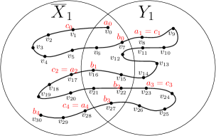
Figure 1: The path $P=\{v_{0},\dots,v_{30}\}$ is illustrated in black. Here $\mathcal{X}=\{0,2,4\}$ correspond to indices $i$ for which $Z_{i}=\overline{X}_{1}$, while $\mathcal{X}=\{1,3\}$ correspond to indices $i$ for which $Z_{i}=$ $Y_{1}$.

We broke $P$ into sub-paths $(x_{a_{0}},\dots,x_{b_{0}}),\dots,(x_{a_{q}},\dots,x_{b_{q}}),\dots,(x_{a_{\bar{q}}},\dots,x_{b_{\bar{q}}})$. For every $q<\bar{q}$, by the maximality of $b_{q}$, $x_{a_{q+1}}\notin Z_{q}$. Furthermore, there is some index $c_{0}\in[a_{0},b_{0}]$ such that $x_{c_{0}}\notin Z_{1}$, as otherwise, $x_{0},\dots,x_{b_{0}},x_{a_{1}}$ are contained in $Z_{1}$, a contradiction to the choice of $b_{0}$. For every $q>0$, set $c_{q}=a_{q}$. Note that for every $q$, $c_{q}\notin Z_{q-1}=Z_{q+1}$. For every pair of vertices $u,v\in X$ such that $u\notin Y_{1}$ and $v\notin\overline{X}_{1}$, it holds that $u\in\underline{X}_{1}$. By the definition of $\overline{X}_{1},\underline{X}_{1}$, it follows that $d_{G[X]}^{{\color[rgb]{1,0,0}(h)}}(u,v)>2\rho_{i}$. In particular, for every $q$, $d_{G}^{{\color[rgb]{1,0,0}(h)}}(x{}_{c_{q}},x{}_{c_{q+1}})>2\rho_{i}$.

For every $q$, using the induction hypothesis on $Z_{q}$, let $x^{\prime}_{a_{q}},\dots,x^{\prime}_{b_{q}}$ be vertices such that $x^{\prime}_{j}\in f(x_{j})$, and $\sum_{j=a_{q}}^{b_{q}}d_{U}(x^{\prime}_{j},x^{\prime}_{j+1})\leq 2t\cdot\log_{\nicefrac{{3}}{{2}}}\mu(Z_{q})\cdot\sum_{j=a_{q}}^{b_{q}}d_{G[X]}(x{}_{j},x{}_{j+1})$. Let $\mathcal{X}\subseteq[0,\bar{q}]$ be all the indices that correspond to $Z_{q}=\overline{X}_{1}$, and $\mathcal{Y}=[0,\bar{q}]\backslash\mathcal{X}$ the indices corresponding to $Z_{q}=Y_{1}$. Note that $\mathcal{X}$ is all the even (or odd) indices. For simplicity of notation we will identify the index $-1$ with $0$, and $m+1$ with $m$. Then

$$\sum_{j=0}^{m-1}d_{U}(x^{\prime}_{j},x^{\prime}_{j+1}) =\sum_{q\in\mathcal{X}}\sum_{j=a_{q}-1}^{b_{q}}d_{U}(x^{\prime}_{j},x^{\prime}_{j+1})+\sum_{q\in\mathcal{\mathcal{Y}}}\sum_{j=a_{q}}^{b_{q}-1}d_{U}(x^{\prime}_{j},x^{\prime}_{j+1})\leavevmode\nobreak\ .$$ (4)

We first bound the second sum in eq. (4), by the induction hypothesis: $\sum_{q\in\mathcal{\mathcal{Y}}}\sum_{j=a_{q}}^{b_{q}-1}d_{U}(x^{\prime}_{j},x^{\prime}_{j+1})\leq 2t\cdot\log_{\nicefrac{{3}}{{2}}}\mu(Y_{1})\cdot\sum_{q\in\mathcal{\mathcal{Y}}}\sum_{j=a_{q}}^{b_{q}-1}d_{G}(x{}_{j},x{}_{j+1})\leq 2t\cdot\log_{\nicefrac{{3}}{{2}}}\mu(X)\cdot\sum_{q\in\mathcal{\mathcal{Y}}}\sum_{j=a_{q}}^{b_{q}-1}d_{G}(x{}_{j},x{}_{j+1})$. For the first sum in eq. (4), as $P$ is ${\color[rgb]{1,0,0}h}$-respecting, for every $q\in\mathcal{X}$, it holds that

$$\sum_{j=a_{q}}^{b_{q}}d_{G}(x{}_{j},x{}_{j+1})\geq d_{G[P]}(x_{c_{q}},x_{c_{q+1}})\geq d_{G}^{{\color[rgb]{1,0,0}(h)}}(x_{c_{q}},x_{c_{q+1}})>2\rho_{i}=\frac{2^{i}}{8(k+1)}=\frac{2^{i}}{t}\leavevmode\nobreak\ .$$

As the maximal possible distance in $U$ is $2^{i}$, using the induction hypothesis, we get

$$\sum_{j=a_{q}-1}^{b_{q}}d_{U}(x^{\prime}_{j},x^{\prime}_{j+1})$$

$$\qquad\leq d_{U}(x^{\prime}_{a_{q}-1},x^{\prime}_{a_{q}})+\sum_{j=a_{q}}^{b_{q}-1}d_{U}(x^{\prime}_{j},x^{\prime}_{j+1})+d_{U}(x^{\prime}_{b_{q}},x^{\prime}_{b_{q}+1})$$

$$\qquad\leq 2^{i}+t\cdot 2\log_{\nicefrac{{3}}{{2}}}\mu(\overline{X}_{1})\cdot\sum_{j=a_{q}}^{b_{q}-1}d_{G}(x{}_{j},x{}_{j+1})+2^{i}$$

$$\qquad\leq\left(t+2t\cdot\log_{\nicefrac{{3}}{{2}}}\left(\frac{2}{3}\mu(X)\right)+t\right)\cdot\sum_{j=a_{q}}^{b_{q}}d_{G}(x{}_{j},x{}_{j+1})=2t\cdot\log_{\nicefrac{{3}}{{2}}}\mu(X)\cdot\sum_{j=a_{q}}^{b_{q}}d_{G}(x{}_{j},x{}_{j+1})\leavevmode\nobreak\ .$$

We conclude

$$\sum_{j=0}^{m-1}d_{U}(x^{\prime}_{j},x^{\prime}_{j+1}) \leq 2t\cdot\log_{\nicefrac{{3}}{{2}}}\mu(X)\cdot\left(\sum_{q\in\mathcal{X}}\sum_{j=a_{q}}^{b_{q}}d_{G}(x{}_{j},x{}_{j+1})+\sum_{q\in\mathcal{\mathcal{Y}}}\sum_{j=a_{q}}^{b_{q}-1}d_{G}(x{}_{j},x{}_{j+1})\right)$$

$$\leq 2t\cdot\log_{\nicefrac{{3}}{{2}}}\mu(X)\cdot\sum_{j=0}^{m-1}d_{U}(x{}_{j},x{}_{j+1})\leavevmode\nobreak\ .$$

∎

Remark 1.

Similarly to [BM04], in cases where $\phi\ll\log n$, one can improve the distortion upper bound in Lemma 9 to $O(k\cdot\phi)$. The proof technique is the same, where we prove by induction that the one-to-many embedding created for scale $2^{i}$ has hop path distortion $(2t\cdot i,{\color[rgb]{1,0,0}h})$.

Finally, we turn to bound $\mathbb{E}_{x\sim\mu}[|f(x)|]$. For a cluster $\underline{X}$, denote by $H(X)$ the graph at the time of the creation of $\underline{X},X,\overline{X}$.

Lemma 10.

For a cluster $X$, created w.r.t. scale $2^{i}$,
it holds that $\mathbb{E}_{x\sim X}[|f(x)|]\leq\mu(X)\cdot\mu\left(B_{H(X)}^{{\color[rgb]{1,0,0}(i\cdot h^{\prime})}}(r(X),2^{i-3})\right)^{\frac{1}{k}}$.

Proof.

We prove the lemma by induction on $i$. Consider first the base case where the cluster $X$ created with scale $i=0$, or more generally, when $X$ is a singleton $\{v\}$. The embedding will be into a single vertex. In particular, $\mathbb{E}_{x\sim X}[|f(x)|]=\mu(\{v\})\leq\mu(X)\cdot\mu\left(B_{H(X)}^{{\color[rgb]{1,0,0}(0)}}(r(X),2^{-3})\right)^{\frac{1}{k}}$. Next we assume that the claim holds for every cluster $X$ which was created during a call to clan-cover with scale $2^{i}$. Consider cluster $X$ on which we call $\texttt{clan-cover}(G[X],\mu,{\color[rgb]{1,0,0}h},k,2^{i+1})$, where $X$ was crated from the graph $H(X)$, and has center $r(X)$ (for the case $i+1=\phi$, let $H(X)=V$, and $r(x)$ to be the vertex maximizing $\mu\left(B_{H(X)}^{{\color[rgb]{1,0,0}(\phi\cdot h^{\prime})}}(r(X),2^{\phi-2})\right)$ ).

Then we called $\texttt{clan-cover}(G[X],\mu,{\color[rgb]{1,0,0}h},k,2^{i})$, and obtain clusters $\overline{X}_{1},\dots,\overline{X}_{s}$, each with center $v_{q}$, that was created when the graph was $Y_{q-1}$. In particular, there is a sub-cluster $\underline{X}_{q}$ such that $Y_{q}=Y_{q-1}\backslash\underline{X}_{q}$. Note that each vertex $v\in X$ belongs to exactly one sub-cluster $\underline{X}_{q}$, hence

$$\sum_{q=1}^{s}\mu(\underline{X}_{q})=\mu(X)$$ (5)

By our choice of index in algorithm 7, for every $q$ it holds that

$$\mu(\overline{X}_{q})\leq\mu(\underline{X}_{q})\cdot\left(\frac{\mu\left(B_{Y_{q-1}}^{{\color[rgb]{1,0,0}((i+1)\cdot h^{\prime})}}(v_{q},2^{i-2})\right)}{\mu\left(B_{Y_{q-1}}^{{\color[rgb]{1,0,0}(i\cdot h^{\prime})}}(v_{q},2^{i-3})\right)}\right)^{\frac{1}{k}}\leavevmode\nobreak\ .$$ (6)

For every $q$, as $Y_{q-1}\subseteq X\subseteq H(X)$, and by the choice of $r(X)$ as the vertex maximizing $\mu\left(B_{H(X)}^{{\color[rgb]{1,0,0}(i\cdot h^{\prime})}}(r(X),2^{i-2})\right)^{\frac{1}{k}}$, it holds that

$$\mu\left(B_{Y_{q+1}}^{{\color[rgb]{1,0,0}((i+1)\cdot h^{\prime})}}(v_{q},2^{i-2})\right)\leq\mu\left(B_{H(X)}^{{\color[rgb]{1,0,0}((i+1)\cdot h^{\prime})}}(v_{q},2^{i-2})\right)\leq\mu\left(B_{H(X)}^{{\color[rgb]{1,0,0}((i+1)\cdot h^{\prime})}}(r(X),2^{i-2})\right)\leavevmode\nobreak\ .$$ (7)

Using the induction, for every $q$ we obtain

$$\mathbb{E}_{x\sim\overline{X}_{q}}[|f_{q}(x)|] \leq\mu(\overline{X}_{q})\cdot\mu\left(B_{Y_{q-1}}^{{\color[rgb]{1,0,0}(i\cdot h^{\prime})}}(v_{q},2^{i-3})\right)^{\frac{1}{k}}$$

$$\overset{(\ref{eq:ClanMeasureClusterIneq})}{\leq}\mu(\underline{X}_{q})\cdot\left(\frac{\mu\left(B_{Y_{q-1}}^{{\color[rgb]{1,0,0}((i+1)\cdot h^{\prime})}}(v_{q},2^{i-2})\right)}{\mu\left(B_{Y_{q-1}}^{{\color[rgb]{1,0,0}(i\cdot h^{\prime})}}(v_{q},2^{i-3})\right)}\right)^{\frac{1}{k}}\cdot\mu\left(B_{Y_{q-1}}^{{\color[rgb]{1,0,0}(i\cdot h^{\prime})}}(v_{q},2^{i-3})\right)^{\frac{1}{k}}$$

$$=\mu(\underline{X}_{q})\cdot\mu\left(B_{Y_{q-1}}^{{\color[rgb]{1,0,0}((i+1)\cdot h^{\prime})}}(v_{q},2^{i-2})\right)^{\frac{1}{k}}$$

$$\overset{(\ref{eq:ClanMusureOfSuperVertex})}{\leq}\mu(\underline{X}_{q})\cdot\mu\left(B_{H(X)}^{{\color[rgb]{1,0,0}((i+1)\cdot h^{\prime})}}(r(X),2^{i-2})\right)^{\frac{1}{k}}\leavevmode\nobreak\ .$$

As $f=\cup_{q=1}^{s}f_{i}$, we conclude

$$\mathbb{E}_{x\sim X}[|f(x)|] =\sum_{q=1}^{s}\mathbb{E}_{x\sim X}[|f_{q}(x)|]$$

$$\leq\sum_{q=1}^{s}\mu(\underline{X}_{q})\cdot\mu\left(B_{H(X)}^{{\color[rgb]{1,0,0}((i+1)\cdot h^{\prime})}}(r(X),2^{i-2})\right)^{\frac{1}{k}}$$

$$\overset{(\ref{eq:SubClustersPartition})}{=}\mu(X)\cdot\mu\left(B_{H(X)}^{{\color[rgb]{1,0,0}((i+1)\cdot h^{\prime})}}(r(X),2^{i-2})\right)^{\frac{1}{k}}\leavevmode\nobreak\ .$$

∎

Using Lemma 10 on $V$ with $i=\phi$ we have $\mathbb{E}_{x\sim V}[|f(x)|]\leq\mu(V)\cdot\mu\left(B_{G}^{{\color[rgb]{1,0,0}(\phi\cdot h^{\prime})}}(r(V),2^{\phi-3})\right)^{\frac{1}{k}}\leq\mu(V)^{1+\frac{1}{k}}$. Lemma 7 now follows by combining Lemma 8, Lemma 9, and Lemma 10.

An observation that will be useful in some of our applications is the following:

Observation 4.

Suppose that Lemma 7 is applied on a measure $\mu$ where for some vertex $r\in V$, $\mu(r)>\frac{1}{2}\mu(V)$. Then in the resulting clan embedding $(f,\chi)$ it will hold that $|f(r)|=1$.

Proof.

Note that in Algorithm 6, we pick a center $v_{1}$ that maximizes $\mu\left(B_{H}^{{\color[rgb]{1,0,0}(i\cdot h^{\prime})}}(v,2^{i-3})\right)$. Note that every ball containing $r$ have measure larger than $\frac{1}{2}\mu(V)$, while every ball that does not contain $r$ has measure less than $\frac{1}{2}\mu(V)$. Thus necessarily $r\in B_{H}^{{\color[rgb]{1,0,0}(i\cdot h^{\prime})}}(v,2^{i-3})$. Next, observe that for every index $j(v_{q})$ chosen in algorithm 7 it will holds that $B_{H}^{{\color[rgb]{1,0,0}(i\cdot h^{\prime})}}(v,2^{i-3})\subseteq\underline{X}_{1}$. Hence $r\notin Y_{1}$, and therefore will not be duplicated: i.e. $r$ belong only to $\overline{X}_{1}$ among all the created clusters. The observation follows now by induction. ∎

4.2 Alternative clan embedding

Similarly to Section 3.2, we provide here an alternative version of Theorem 3, providing a hop-distortion of $\left(O(k\cdot\log\log n),{\color[rgb]{1,0,0}O(k\cdot\log\log n)},{\color[rgb]{1,0,0}h}\right)$, in addition, the polynomial aspect ratio assumption is removed. The only change compared with the Hop-constrained-clan-embedding algorithm will be in the Clan-create-cluster procedure. See 4

As usual, the most crucial step will be to deal with the distributional case:

Lemma 11.

Consider an $n$-vertex graph $G=(V,E,w)$ with polynomial aspect ratio, $(\geq 1)$-measure $\mu:X\rightarrow\mathbb{R}_{\geq 1}$, and parameters $k,{\color[rgb]{1,0,0}h}\in[n]$. Then there is a clan embedding $(f,\chi)$ into an ultrametric with hop-distortion $\left(O(k\cdot\log\log\mu(V)),{\color[rgb]{1,0,0}O(k\cdot\log\log\mu(V))},{\color[rgb]{1,0,0}h}\right)$, hop-path-distortion $\left({O(k\cdot\log\mu(V)\cdot\log\log\mu(V))},{\color[rgb]{1,0,0}h}\right)$, and such that $\mathbb{E}_{v\sim\mu}[|f(v)|]\leq\mu(V)^{1+\frac{1}{k}}$.

The proof of Theorem 4 using Lemma 11 follows the exact same lines as the proof of Theorem 3 using Lemma 7, and thus we will skip it.

4.3 Proof of Lemma 11: alternative distributional h.c. clan embedding

For the embedding of Lemma 11 we will use the exact same Hop-constrained-clan-embedding (Algorithm 5), with the only difference that instead of using the Clan-create-Cluster procedure (Algorithm 7), we will use the Clan-create-cluster-alt procedure (Algorithm 8). Similarly to the proof of Lemma 7 we will assume that $\mathrm{diam}^{{\color[rgb]{1,0,0}(h)}}(G)<\infty$. The exact same argument from Section 3.1.1 can be used to remove this assumption. We begin by making the call Hop-constrained-clan-embedding$(G[V],\mu,{\color[rgb]{1,0,0}h},k,2^{\phi})$, where the call to Clan-create-Cluster in algorithm 6 of Algorithm 6 is replaced by a call to Clan-create-cluster-alt.

input : Induced graph $G[Y]$, parameters ${\color[rgb]{1,0,0}h},k\in\mathbb{N}$, $\geq 1$-measure $\mu$, scale $i$.

output : Three clusters $(\underline{A},A,\overline{A})$, where $\underline{A}\subseteq A\subseteq\overline{A}$.

1 set $L=\lceil 1+\log\log\mu(Y)\rceil$ and $\Delta=2^{i}$

2 let $v\in V(H)$ with minimal $\mu\left(B_{Y}^{{\color[rgb]{1,0,0}(2k\cdot L\cdot h)}}(v,\frac{1}{4}\Delta)\right)$

3 if $\mu\left(B_{Y}^{{\color[rgb]{1,0,0}(2k\cdot L\cdot h)}}(v,\frac{1}{4}\Delta)\right)>\frac{1}{2}\cdot\mu_{M}(Y)$ then

       return $(X,X,X)$

        // Note that for every $u,v\in X$, $d_{H}^{{\color[rgb]{1,0,0}(4k\cdot L\cdot h)}}(u,v)\leq\frac{\Delta}{2}$

4      

5denote $A_{a,j}=B_{Y}^{{\color[rgb]{1,0,0}((2k\cdot a+j)\cdot h)}}\left(v,(a+\frac{j}{2k})\cdot\frac{\Delta}{4L}\right)$

6 let $a\in[0,L-1]$ such that $\mu\left(A_{a,0}\right)\geq\frac{\mu\left(A_{a+1,0}\right)^{2}}{\mu(H)}$

7 let $j\in[0,2(k-1)]$ such that $\mu\left(A_{a,j+2}\right)\leq\mu\left(A_{a,j}\right)\cdot\left(\frac{\mu\left(A_{a+1,0}\right)}{\mu\left(A_{a,0}\right)}\right)^{\frac{1}{k}}$

8 return $(A_{a,j},A_{a,j+1},A_{a,j+2})$

Algorithm 8 $(\underline{A},A,\overline{A})=\texttt{Clan-create-cluster-alt}(G[Y],\mu,{\color[rgb]{1,0,0}h},k,2^{i})$

The proofs of the following two claims and observation are identical to these of 3, 4, and 2, so we will skip them.

Claim 7.

In algorithm 8 of Algorithm 8, there is an index $a\in[0,L-1]$ such that $\mu\left(A_{a,0}\right)\geq\frac{\mu\left(A_{a+1,0}\right)^{2}}{\mu(H)}$.

Claim 8.

In algorithm 8 of Algorithm 8, there is an index $j\in[0,2(k-1)]$ such that $\mu_{M}\left(A_{a,j+2}\right)\leq\mu_{M}\left(A_{a,j}\right)\cdot\left(\frac{\mu_{M}\left(A_{a+1,0}\right)}{\mu_{M}\left(A_{a,0}\right)}\right)^{\frac{1}{k}}$.

Observation 5.

Every cluster $X$ on which we execute the Hop-constrained-clan-embedding with scale $2^{i}$ has diameter at most $\mathrm{diam}^{{\color[rgb]{1,0,0}(4k\cdot L\cdot h)}}(G[X])\leq 2^{i}$.

The proof of the following lemma follows the same lines as Lemma 8, and we will skip it.

Lemma 12.

The clan embedding $(f,\chi)$ has hop-distortion $(O(k\cdot\log\log\mu(V)),{\color[rgb]{1,0,0}O(k\cdot\log\log\mu(V))},{\color[rgb]{1,0,0}h})$.

Our next goal is to prove the path distortion guarantee (parallel to Lemma 9). We observe the following:

Observation 6.

Consider a cluster $\overline{A}$ returned by the call Clan-create-cluster-alt$(G[Y],\mu,{\color[rgb]{1,0,0}h},k,2^{i})$. Then either $\overline{A}=\underline{A}=Y$, or $\mu(\overline{A})\leq\frac{1}{2}\mu(Y)$.

Proof.

Consider the execution of the Clan-create-cluster-alt procedure on input $(G[Y],\mu,{\color[rgb]{1,0,0}h},k,2^{i})$. If the algorithm halts in algorithm 8, then $\overline{A}=\underline{A}=Y$ and we are done. Otherwise, we have that $\mu\left(B_{H}^{{\color[rgb]{1,0,0}(2k\cdot L\cdot h)}}(v,\frac{1}{4}\Delta)\right)\leq\frac{1}{2}\cdot\mu_{M}(Y)$, while $\overline{A}=A_{a,j+2}$ for some $a\leq L-1$ and $j\leq 2(k-1)$. Hence $A_{a,j+2}\subseteq A_{L-1,2k}=B_{H}^{{\color[rgb]{1,0,0}((2k\cdot(L-1)+2k)\cdot h)}}\left(v,(L-1+\frac{2k}{2k})\cdot\frac{\Delta}{4L}\right)=B_{H}^{{\color[rgb]{1,0,0}(2k\cdot L\cdot h)}}\left(v,\frac{\Delta}{4}\right)$, implying that $\mu(\overline{A})\leq\frac{1}{2}\cdot\mu_{M}(Y)$, as required. ∎

Given 6, the proof of the following theorem follow the exact same lines as Lemma 9 (replacing $O(k)$ with $O(k\cdot\log\log\mu(X))$), and we will skip it (note that Remark 1 will also hold).

Lemma 13.

The one-to-many embedding $f$ has hop path distortion $\left({O(k\cdot\log\mu(V)\cdot\log\log\mu(V))},{\color[rgb]{1,0,0}h}\right)$.

Finally, we turn to bound $\mathbb{E}_{x\sim\mu}[|f(x)|]$. Recall that for a cluster $\underline{X}$, we denote by $H(X)$ the graph at the time of the creation of $\underline{X},X,\overline{X}$.

Lemma 14.

It holds that $\mathbb{E}_{v\sim V}[|f(v)|]\leq\mu(V)^{1+\frac{1}{k}}$.

Proof.

We prove the lemma by induction on $i$ and $|X|$. Specifically, the induction hypothesis is that for a cluster $X$, created w.r.t. scale $2^{i}$, it holds that $\mathbb{E}_{x\sim X}[|f(x)|]\leq\mu(X)^{1+\frac{1}{k}}$. Consider first the base case where the cluster $X$ created with scale $i=0$, or when $X$ is a singleton $\{v\}$. The embedding will be into a single vertex. In particular, $\mathbb{E}_{x\sim X}[|f(x)|]=\mu(\{v\})\leq\mu\left(X\right)^{1+\frac{1}{k}}$.

Next we assume that the claim holds for every cluster $X$ which was created during a call to Hop-constrained-clan-embedding with scale $2^{i-1}$. Consider cluster $X$ on which we call $\texttt{Hop-constrained-clan-embedding}(G[X],\mu,{\color[rgb]{1,0,0}h},k,2^{i})$. Then we called $\texttt{clan-cover}(G[X],\mu,{\color[rgb]{1,0,0}h},k,2^{i})$, and obtain clusters $\overline{X}_{1},\dots,\overline{X}_{s}$. Then for each cluster $\overline{X}_{q}$ it creates a one-to-many embedding $f_{q}$. If $s=1$, then there is only a single cluster and the lemma will follow by the induction hypothesis on $i-1$. Else, we obtain a non-trivial cover. Recall that after creating $\overline{X}_{1}$, the set of remaining vertices is denoted $Y_{1}=X\backslash\underline{X}_{1}$. Note that if we were to call clan-cover on input $(G[Y_{1}],\mu,{\color[rgb]{1,0,0}h},k,2^{i})$, the algorithm will first create a cover $\overline{X}_{2},\dots,\overline{X}_{s}$ of $Y_{1}$, and then will recursively create one-to-many embeddings for each $\overline{X}_{q}$. Denote by $\tilde{f}$ the one-to-many embedding created by such a call. It holds that $f=f_{1}\cup\tilde{f}$. Therefore, we can analyze the rest of the process as if the algorithm did a recursive call on $Y_{1}$ rather than on each cluster $\overline{X}_{q}$. Since $|\overline{X}_{1}|,|Y_{1}|<|X|$, the induction hypothesis implies that $\mathbb{E}_{x\sim\overline{X}_{1}}[|f_{1}(x)|]\leq\mu(\overline{X}_{1})^{1+\frac{1}{k}}$ and $\mathbb{E}_{x\sim Y_{1}}[|\tilde{f}(x)|]\leq\mu(Y_{1})^{1+\frac{1}{k}}$. As the Padded-partition algorithm did not returned a trivial partition of $X$, it defined $A_{a,j}=B_{H}^{{\color[rgb]{1,0,0}((2k\cdot a+j)\cdot h)}}\left(v,(a+\frac{j}{2k})\cdot\frac{\Delta}{4L}\right)$, and returned $(\underline{X}_{1},X_{1},\overline{X}_{1})=(A_{a,j},A_{a,j+1},A_{a,j+2})$. The indices $a,j$ where chosen such that $\mu\left(A_{a,0}\right)\geq\frac{\mu\left(A_{a+1,0}\right)^{2}}{\mu(X)}$ and $\mu\left(A_{a,j+2}\right)\leq\mu\left(A_{a,j}\right)\cdot\left(\frac{\mu\left(A_{a+1,0}\right)}{\mu\left(A_{a,0}\right)}\right)^{\frac{1}{k}}$, implying

$$\mu\left(\overline{X}_{1}\right)\leq\mu\left(\underline{X}_{1}\right)\cdot\left(\frac{\mu\left(A_{a+1,0}\right)}{\mu\left(A_{a,0}\right)}\right)^{\frac{1}{k}}\leq\mu\left(\underline{X}_{1}\right)\cdot\left(\frac{\mu\left(X\right)}{\mu\left(A_{a+1,0}\right)}\right)^{\frac{1}{k}}\leavevmode\nobreak\ .$$

It follows

$$\mathbb{E}_{x\sim\overline{X}_{1}}[|f_{1}(x)|] \leq\mu(\overline{X}_{1})^{1+\frac{1}{k}}=\mu(\overline{X}_{1})\cdot\mu(\overline{X}_{1})^{\frac{1}{k}}$$

$$\leq\mu\left(\underline{X}_{1}\right)\cdot\left(\frac{\mu\left(X\right)}{\mu\left(A_{a+1,0}\right)}\right)^{\frac{1}{k}}\cdot\mu(\overline{X}_{1})^{\frac{1}{k}}\leq\mu\left(\underline{X}_{1}\right)\cdot\mu\left(X\right)^{\frac{1}{k}}\leavevmode\nobreak\ ,$$

where the last inequality follows as $A_{a+1,0}\supseteq A_{a,j+2}=\overline{X}_{1}$. As $X=\underline{X}_{1}\cupdot Y_{1}$, we conclude

$$\mathbb{E}_{x\sim X}[|f(x)|] =\mathbb{E}_{x\sim\overline{X}_{1}}[|f_{1}(x)|]+\mathbb{E}_{x\sim Y_{1}}[|\tilde{f}(x)|]\leq\mu\left(\underline{X}_{1}\right)\cdot\mu\left(X\right)^{\frac{1}{k}}+\mu\left(Y_{1}\right)\cdot\mu\left(X\right)^{\frac{1}{k}}=\mu\left(X\right)^{1+\frac{1}{k}}\leavevmode\nobreak\ .$$

∎

Lemma 11 now follows by combining Lemma 12, Lemma 13, and Lemma 14.

An observation that will be useful in some of our applications is the following:

Observation 7.

Suppose that Lemma 11 is applied on a measure $\mu$ where for some vertex $r\in V$, $\mu(r)>\frac{1}{2}\mu(V)$. Then in the resulting clan embedding $(f,\chi)$ it will hold that $|f(r)|=1$.

Proof.

Consider an execution of the Clan-create-cluster-alt$(G[Y],\mu,{\color[rgb]{1,0,0}h},k,2^{i})$ (Algorithm 8) procedure where $r\in Y$. The algorithm picks a center $v$ that minimizes $\mu\left(B_{Y}^{{\color[rgb]{1,0,0}(2k\cdot L\cdot h)}}(v,\frac{1}{4}\Delta)\right)$. Note that every ball containing $r$ have measure strictly larger then $\frac{1}{2}\mu(V)$, while every ball that does not contain $r$ has measure strictly less than $\frac{1}{2}\mu(V)$. Thus by 6, either $\underline{A}=Y$, or $\mu(\overline{A})\leq\frac{1}{2}\mu(Y)$, which implies $r\notin\overline{A}$. If follows that in any call to the clan-cover procedure that returns $(\overline{X}_{1},\dots,\overline{X}_{s})$, $r$ will belong only to $\overline{X}_{s}$. The observation now follows by induction. ∎

5 Subgraph preserving one-to-many embedding

In this section we will modify our clan embeddings so that they will produce (non-tree) sub-graphs version. In particular, we will obtain that every “hop-bounded” subgraph of $G$ has a “copy” in the image. We begin with some definitions for hop-bounded tree embedding (very similar definition was defined by [HHZ21b]). See Figure 2 for illustration.

Definition 8 (Path Tree One-To-Many Embedding).

A one-to-many path tree embedding on weighted graph $G=(V,E,w_{G})$ consists of a dominating one-to-many embedding $f$ into a tree $T$ such that $f(V)=V(T)$, and associated paths $\{P^{T}_{e}\}_{e\in E(T)}$, where for every edge $e=\{u^{\prime},v^{\prime}\}\in E(T)$ where $u^{\prime}\in f(u)$ and $v^{\prime}\in f(v)$, $P^{T}_{e}$ is a path from $u$ to $v$ in $G$ of weight at most $w_{T}(\{u^{\prime},v^{\prime}\})$.

For every two vertices $u^{\prime},v^{\prime}\in V(T)$, let $e_{1},e_{2},\dots,e_{s}$ be the unique simple path between them in $T$. We denote: $P^{T}_{u^{\prime}v^{\prime}}=P^{T}_{e_{1}}\circ P^{T}_{e_{2}}\circ\cdots\circ P^{T}_{e_{s}}$ to be the concatenation of all the associated paths (note that $P^{T}_{u^{\prime}v^{\prime}}$ is not necessarily simple). We say that $f$ has hop-bound $\beta$ if for every $u^{\prime},v^{\prime}\in V(T)$ which are connected in $T$, $\mathrm{hop}(P^{T}_{u^{\prime}v^{\prime}})\leq\beta$.

Figure 2: The graph $G$ is illustrated on the left, while the path tree one-to-many embedding into the tree $T$ is illustrated on the right. Each edge $e\in T$ has an associated path $P^{T}_{e}$, for example $P^{T}_{e^{\prime},d}=(e,d)$, and $P^{T}_{a^{\prime},e}=(a,f,e)$. Each pair of vertices $u,v\in V(T)$, has an (not necessarily simple) induced path $P^{T}_{u,v}$, for example $P^{T}_{f,e^{\prime}}=(f,b,c,d,e)$, and $P^{T}_{a^{\prime},e^{\prime}}=(a,f,e,b,c,d,e)$. The hop-bound $\beta$ is the maximal number of hops in an inducted path. Here $\beta=6$ (realized by $P_{T}^{a^{\prime},e^{\prime}}$).

First, we translate Lemma 7 to the language of path tree embeddings.

Lemma 15.

Given an $n$-point weighted graph $G=(V,E,w_{G})$ with polynomial aspect ratio, a vertex $r\in V$, and integer ${\color[rgb]{1,0,0}h}\geq 1$, there is a dominating clan embedding $(f,\chi)$ into a tree $T$ such that:

1. $|f(V)|=O(n^{1.5})$ and $|f(r)|=1$.

2. $(f,\chi)$ has hop-distortion $\left(O(1),{\color[rgb]{1,0,0}O(\log n)},{\color[rgb]{1,0,0}h}\right)$, and hop-path-distortion $\left({O(\log n)},{\color[rgb]{1,0,0}h}\right)$.

3. $f$ is a path tree one-to-many embedding with associated paths $\{P^{T}_{e}\}_{e\in E(T)}$ and hop-bound ${\color[rgb]{1,0,0}O(\log^{2}n)\cdot h}$.

Proof.

First apply Lemma 7 on the graph $G=(V,E,w)$ with parameter ${\color[rgb]{1,0,0}h}$, $k=2$, and $(\geq 1)$-measure $\mu$ where $\mu(r)=n$, and for every $v\neq r$, $\mu(v)=1$. As a result we will obtain a dominating clan embedding $(f_{U},\chi_{U})$ into an ultrametric $U$, where (1) $|f_{U}(V)|\leq\mu(V)^{1+\frac{1}{2}}=O(n^{1.5})$, (2) $\forall u,v\in V$, $d_{G}^{{\color[rgb]{1,0,0}(O(\log n)\cdot h)}}(u,v)\leq\min_{v^{\prime}\in f_{U}(v),u^{\prime}\in f_{U}(u)}d_{U}(v^{\prime},u^{\prime})$, (3) $\forall u,v\in V$, $\min_{v^{\prime}\in f_{U}(v)}d_{U}(v^{\prime},\chi(u))\leq 48\cdot d_{G}^{{\color[rgb]{1,0,0}(h)}}(u,v)$, (4) $f$ has hop-path distortion $\left(O(\log n),{\color[rgb]{1,0,0}h}\right)$, and finally, (5) as $\mu(r)>\frac{1}{2}\mu(V)$, 4 implies that $|f_{U}(r)|=1$.

Next, we transform the ultrametric into a tree. Gupta [Gup01], showed that given a tree $\mathcal{T}$ and a subset of terminals $K\subseteq V(\mathcal{T})$, one can (efficiently) embed (in a classic one-to-one fashion) the set of terminals $K$ into a tree $\mathcal{T}_{K}$ such that $V(\mathcal{T}_{K})=K$, and for every $u,v\in K$, $d_{\mathcal{T}}(u,v)\leq d_{\mathcal{T}_{K}}(u,v)\leq 8\cdot d_{\mathcal{T}}(u,v)$. Applying [Gup01] on the ultrametric $U$ with $f_{U}(V)$ as the set of terminals $K$, and concatenating the two embeddings, we obtain a clan embedding $(f,\chi)$ into a tree $\mathcal{T}_{K}$ over $f_{U}(V)$ such that $\forall u,v\in V$,

$$d_{G}^{{\color[rgb]{1,0,0}(O(\log n)\cdot h)}}(u,v) \leq\min_{v^{\prime}\in f(v),u^{\prime}\in f(u)}d_{\mathcal{T}_{K}}(v^{\prime},u^{\prime})$$

$$\min_{v^{\prime}\in f(v)}d_{\mathcal{T}_{K}}(v^{\prime},\chi(u)) \leq 48\cdot 8\cdot d_{G}^{{\color[rgb]{1,0,0}(h)}}(u,v)\leavevmode\nobreak\ .$$

For every sequence of vertices $v^{\prime}_{0},\dots,v^{\prime}_{s}$ in $f_{U}(V)$, it holds that $\sum_{i=0}^{s-1}d_{\mathcal{T}_{K}}(v^{\prime}_{i},v^{\prime}_{i+1})\leq 8\cdot\sum_{i=1}^{s-1}d_{U}(v^{\prime}_{i},v^{\prime}_{i+1})$. As $f_{U}$ has path distortion ${\color[rgb]{1,0,0}O(\log n)}$, if follows that $f$ has path distortion ${\color[rgb]{1,0,0}O(\log n)}$ as well.

Finally, for every edge $e=\{u^{\prime},v^{\prime}\}\in E(T)$ where $u^{\prime}\in f(u)$ and $v^{\prime}\in f(v)$, let $P^{\mathcal{T}_{K}}_{e}$ be a path of minimum weight among all the $u$-$v$ paths in $G$ with at most ${\color[rgb]{1,0,0}O(\log n)\cdot h}$ hops. Note that $w_{G}(P_{e}^{\mathcal{T}_{K}})\leq d_{G}^{{\color[rgb]{1,0,0}(O(\log n)\cdot h)}}(u,v)\leq d_{\mathcal{T}_{K}}(u^{\prime},v^{\prime})$. Following Algorithm 5, as $G$ has polynomial aspect ratio, the ultrametric $U$ has depth $O(\log n)$. In particular, every path in $U$ consists of at most ${\color[rgb]{1,0,0}O(\log n)}$ hops. The tree $\mathcal{T}_{K}$ constructed by [Gup01] (see also [FKT19]) is a minor of $U$ constructed by contracting edges only. Therefore, the hop-diameter of $\mathcal{T}_{K}$ is bounded by ${\color[rgb]{1,0,0}O(\log n)}$ as well. Consider $u^{\prime},v^{\prime}\in f(V)$, then $P^{\mathcal{T}_{K}}_{u^{\prime}v^{\prime}}$ consist of concatenating at most $O(\log n)$ paths, each with ${\color[rgb]{1,0,0}O(\log n)\cdot h}$ hops. It follows that $\mathrm{hop}(P^{\mathcal{T}_{K}}_{u^{\prime}v^{\prime}})\leq{\color[rgb]{1,0,0}O(\log^{2}n)\cdot h}$ as required. ∎

Recall that a subgraph $H$ of $G$ is ${\color[rgb]{1,0,0}h}$-respecting if for every $u,v\in H$. It holds that $d^{{\color[rgb]{1,0,0}(h)}}_{G}(u,v)\leq d_{H}(u,v)$, The following is a corollary of Lemma 15.

Corollary 1.

Consider an $n$-point graph $G=(V,E,w)$ with polynomial aspect ratio, parameter ${\color[rgb]{1,0,0}h}\in\mathbb{N}$ and vertex $r\in V$. Then there is a path-tree one-to-many embedding $f$ of $G$ into a tree $T$ with hop bound ${\color[rgb]{1,0,0}O(\log^{2}n)\cdot h}$, $|f(V)|=O(n^{1.5})$, $|f(r)|=1$, and such that for every connected ${\color[rgb]{1,0,0}h}$-respecting sub-graph $H$, there is a connected subgraph $H^{\prime}$ of $T$ where for every $u\in H$, $H^{\prime}$ contains some vertex from $f(u)$. Further, $w_{T}(H^{\prime})\leq O(\log n)\cdot w(H)$.

Proof.

We apply Lemma 15 on $G$. All the properties other than the last one hold immediately. Consider an ${\color[rgb]{1,0,0}h}$-respecting subgraph $H$ of $G$. We double each edge in $H$, to obtain a multi-graph, where all the vertex degrees are even. In particular, there is an Eulerian tour $P=(x_{0},\dots,x_{s})$ traversing all the edges in $H$. Note that for every $a,b\in[0,s]$ it holds that

$$d_{P}(x_{a},x_{b})\geq d_{H}(x_{a},x_{b})\geq d^{{\color[rgb]{1,0,0}(h)}}_{G}(x_{a},x_{b})\leavevmode\nobreak\ .$$

Thus $P$ is an ${\color[rgb]{1,0,0}h}$-respecting path. It follows that there are vertices $x^{\prime}_{0},\dots,x^{\prime}_{s}$ where $x^{\prime}_{i}\in f(x_{i})$ such that $\sum_{i=0}^{s-1}d_{T}(x^{\prime}_{i},x^{\prime}_{i+1})\leq O(\log n)\cdot\sum_{i=0}^{s-1}w(v_{i},v_{i+1})=O(\log n)\cdot 2\cdot w(H)$. The corollary follows. ∎

Finally, we will state the result in this section in an alternative form, where instead of Lemma 7, we will use Lemma 11. In Lemma 15 we will obtain the same result with the only changes that $(f,\chi)$ will have hop-distortion $\left(O(\log\log n),{\color[rgb]{1,0,0}O(\log\log n)},{\color[rgb]{1,0,0}h}\right)$, hop-path-distortion $\left({O(\log n\cdot\log\log n)},{\color[rgb]{1,0,0}h}\right)$, and the hop bound of the path tree one-to-many embedding will be ${\color[rgb]{1,0,0}O(\log n\cdot\log\log n)\cdot h}$. The following corollary follow the same lines:

Corollary 2.

Consider an $n$-point graph $G=(V,E,w)$ with polynomial aspect ratio, parameter ${\color[rgb]{1,0,0}h}\in\mathbb{N}$ and vertex $r\in V$. Then there is a path-tree one-to-many embedding $f$ of $G$ into a tree $T$ with hop bound ${\color[rgb]{1,0,0}O(\log n\cdot\log\log n)\cdot h}$, $|f(V)|=O(n^{1.5})$, $|f(r)|=1$, and such that for every connected ${\color[rgb]{1,0,0}h}$-respecting sub-graph $H$, there is a connected subgraph $H^{\prime}$ of $T$ where for every $u\in H$, $H^{\prime}$ contains some vertex from $f(u)$. Further, $w_{T}(H^{\prime})\leq O(\log n\cdot\log\log n)\cdot w(H)$.

5.1 General subgraph

Both Corollary 1 and Corollary 2 have a major drawback: the guarantee is only w.r.t. ${\color[rgb]{1,0,0}h}$-respecting sub-graphs. This is not enough, as for example in our application for the h.c. group Steiner forest, the solution is not necessarily ${\color[rgb]{1,0,0}h}$-respecting. It is impossible to preserve every subgraph, for example if one embeds the path graph $(v_{0},\dots,v_{n})$ with hop parameter ${\color[rgb]{1,0,0}h}=1$, the distance between every pair of copies $v^{\prime}_{0}\in f(v_{0}),v^{\prime}_{n}\in f(v_{n})$ has to be $\infty$. Thus any “image” of the entire graph has to be of weight $\infty$. Here we ensure the next best thing: given a subgraph $H$ of $G$, we will construct a (not necessarily connected) subgraph $H^{\prime}$ of $T$ where for every $u,v\in H$ such that $\mathrm{hop}_{H}(u,v)\leq{\color[rgb]{1,0,0}h}$, $H^{\prime}$ contains a pair of copies $u^{\prime}\in f(u)$ and $v^{\prime}\in f(v)$ in the same connected component. Further, $w_{T}(H^{\prime})\leq O(\log n)\cdot w(H)$. As a result, the hop bound will increase by a $\log$ factor.

See 5

Proof.

Set ${\color[rgb]{1,0,0}h^{\prime}}={\color[rgb]{1,0,0}h\cdot 4\log n}$. We execute Corollary 1 with hop parameter ${\color[rgb]{1,0,0}h^{\prime}}$. As a result we obtain a path-tree one-to-many embedding $f$ into a tree $T$ with hop bound ${\color[rgb]{1,0,0}O(\log^{2}n)\cdot h^{\prime}}={\color[rgb]{1,0,0}O(\log^{3}n)\cdot h}$, $|f(V)|=O(n^{1.5})$, and $|f(r)|=1$. It only remains to prove the subgraph preservation property.

The following lemma will be crucial, the proof and historical context are given in Section 5.2.

Lemma 16 (Sparse Cover).

Consider an $n$-vertex weighted graph $G=(V,E,w)$, with cost function $\mu:E\rightarrow\mathbb{R}_{\geq 0}$, and parameter $\Delta>0$. Then there is a collection of cluster $C_{1},C_{2},\dots,C_{s}$ such that:

1. Each $C_{i}$ has radius at most $\Delta\cdot\log(2n)$. That is, there is a vertex $v_{i}\in C_{i}$ such that $\max_{u\in C_{i}}d_{G[C_{i}]}(u,v_{i})\leq\Delta\cdot\log(2n)$.

2. Every pair of vertices $u,v$ such that $d_{G}(u,v)\leq\Delta$ belongs to some $C_{i}$.

3. $\sum_{i=1}^{s}\mu(C_{i})\leq 4\cdot\mu(G)$, where $\mu(C)=\sum_{e\subseteq C}\mu(e)$.

Consider a subgraph $H=(V_{H},E_{H},w)$ of $G$. Let $H^{\prime}=(V_{H},E_{H})$ be the graph $H$ where all the edge weights were changed to $1$. Set $\Delta={\color[rgb]{1,0,0}h}$. and a cost function $\mu:E_{H}\rightarrow\mathbb{R}_{\geq 0}$, where $\mu(e)=w(e)$. Using Lemma 16, we obtain a collection of clusters $C_{1},\dots,C_{s}$. Let $F_{i}$ be the shortest path tree rooted in $v_{i}$ spanning all the vertices in $C_{i}$, and having the original weights $w$ of $G$. Note that as $H^{\prime}$ is unweighted, every path in $F_{i}$ contains at most $2\cdot\Delta\cdot\log 2n\leq{\color[rgb]{1,0,0}h}\cdot 4\log n={\color[rgb]{1,0,0}h^{\prime}}$ hops. In particular, $F_{i}$ is ${\color[rgb]{1,0,0}h^{\prime}}$-respecting subgraph of $G$. By Corollary 1, there is a connected subgraph $T_{i}$ of $T$ where for every $u\in F_{i}$, $T_{i}$ contains some vertex from $f(u)$. Further, $w_{T}(T_{i})\leq O(\log n)\cdot w(F_{i})$. Set $H^{\prime}=\cup_{i=1}^{s}F_{i}$. Note that for every $u,v\in H$ such that $\mathrm{hop}_{H}(u,v)\leq{\color[rgb]{1,0,0}h}$, it holds that $d_{H^{\prime}}(u,v)\leq{\color[rgb]{1,0,0}h}$, and hence by Lemma 16 there is some cluster $C_{i}$ containing both $u,v$. According to Corollary 1 $T_{i}$ is a connected subgraph containing vertices from both $f(u)$ and $f(v)$, as required. Finally, we bound the weight of $H^{\prime}$:

$$w_{T}(H^{\prime}) \leq\sum_{i=1}^{s}w_{T}(T_{i})=O(\log n)\cdot\sum_{i=1}^{s}w(F_{i})\leq O(\log n)\cdot\sum_{i=1}^{s}w(C_{i})$$

$$=O(\log n)\cdot\sum_{i=1}^{s}\mu(C_{i})=O(\log n)\cdot\mu(H)=O(\log n)\cdot w(H)\leavevmode\nobreak\ .$$

∎

By using Corollary 2 instead of Corollary 1 in the proof above, we obtain the following:

Theorem 11.

Consider an $n$-point graph $G=(V,E,w)$ with polynomial aspect ratio, parameter ${\color[rgb]{1,0,0}h}\in\mathbb{N}$ and vertex $r\in V$. Then there is a path-tree one-to-many embedding $f$ of $G$ into a tree $T$ with hop bound ${\color[rgb]{1,0,0}O(\log^{2}n\cdot\log\log n)\cdot h}$, $|f(V)|=O(n^{1.5})$, $|f(r)|=1$, and such that for every sub-graph $H$, there is a subgraph $H^{\prime}$ of $T$ where for every $u,v\in H$ with $\mathrm{hop}_{H}(u,v)\leq{\color[rgb]{1,0,0}h}$, $H^{\prime}$ contains a pair of copies $u^{\prime}\in f(u)$ and $v^{\prime}\in f(v)$ in the same connected component. Further, $w_{T}(H^{\prime})\leq O(\log n\cdot\log\log n)\cdot w(H)$.

5.2 Proof of Lemma 16: sparse cover

Sparse covers were first introduced by Awerbuch and Peleg [AP90], and were studied for different graph families. We refer to [Fil19a, Fil20] for farther details. For an integer parameter $k\geq 1$, and $\Delta>0$, Awerbuch and Peleg partitioned a general $n$-vertex graph into clusters of radius at most $(2k-1)\cdot\Delta$ such that every ball of radius $\Delta$ is fully contained in some cluster, and every vertex belongs to at most $2k\cdot n^{\frac{1}{k}}$ different clusters. In particular, by fixing $k=\log n$, one will get all the properties in Section 5.2, but the bound on $\sum_{i}\mu(C_{i})$ will only be $4\log n\cdot\mu(G)$. While the construction in [AP90] is deterministic, here we will present a random ball growing clustering algorithm (ala [Bar96]). As a result, while in the worst case a vertex might belong to $\log n$ different clusters, in expectation, each vertex will belong only to a constant number. A bound on the total weight will follow.

Proof of Lemma 16. By scaling, we can assume that $\Delta=1$. Let $\mathsf{Geo}(\frac{1}{2})$ be geometric distribution with parameter $\frac{1}{2}$ (that is getting value $i\geq 1$ with probability $2^{-i}$). Each created cluster $C$ will have an interior part denoted $\mathsf{int}(C)$, that will be contained in $C$. We create a collection of clusters $\mathcal{C}$ as follows, initially $Y_{1}=V$ is all the unclustered vertices. At step $i$, after we created the clusters $C_{1},C_{2},\dots,C_{i-1}$, the unclustered vertices are $Y_{i}=V\setminus(\cup_{j<i}\mathsf{int}(C_{j}))$. Pick an arbitrary vertex $x_{i}\in Y_{i}$, and a radius $r_{i}\sim\mathsf{Geo}(\frac{1}{2})$. Set the new cluster to be $C_{i}=B_{G[Y_{i}]}(x_{i},r_{i})$ the ball of radius $r_{i}$ around $x_{i}$ in the graph induced by the unclustered vertices, and its interior to $\mathsf{int}(C_{i})=B_{G[Y_{i}]}(x_{i},r_{i}-1)$. The process halts once $Y_{i}=\emptyset$. See illustration on the right.

Consider a pair $u,v$ such that $d_{G}(u,v)\leq 1$, and let $P$ be the shortest path between them. Let $i$ be the first index such that $\mathsf{int}(C_{i})\cap P\neq\emptyset$, and let $z\in\mathsf{int}(C_{i})\cap P$. By the minimality of $i$, $P\subseteq Y_{i}$. As $z\in\mathsf{int}(C_{i})$ it follows that $d_{G[Y_{i}]}(x_{i},z)\leq r_{i}-1$. By triangle inequality $d_{G[Y_{i}]}(x_{i},u)\leq d_{G[Y_{i}]}(x_{i},z)+d_{G[Y_{i}]}(z,u)\leq r_{i}$, implying that $u\in C_{i}$. Similarly, $v\in C_{i}$. property (2) of Lemma 16 follows.

The radius of the cluster $C_{i}$ is bounded by $r_{i}$. Denoted by $\Psi$ the event that $r_{i}\leq\log(2n)$ for every $i$. By union bound,

$$\Pr\left[\overline{\Psi}\right]=\Pr\left[\exists i\text{ s.t. }r_{i}>\log(2n)\right]\leq n\cdot 2^{-\log(2n)}=\frac{1}{2}\leavevmode\nobreak\ .$$

Denote by $X_{v}$ the number of cluster containing a vertex $v$. Note that given that $v$ belongs to a cluster $C_{i}$, by the memoryless of geometric distribution, the probability that $v$ belongs to the the interior of the cluster is $\frac{1}{2}$:

$$\Pr\left[v\in\mathsf{int}(C_{i})\mid v\in C_{i}\right]=\Pr\left[d_{G}(x_{i},v)\leq r_{i}-1\mid d_{G}(x_{i},v)\leq r_{i}\right]=\frac{1}{2}\leavevmode\nobreak\ .$$

Once $v$ belongs to the interior of a cluster $\mathsf{int}(C_{i})$, it will not belong to any other clusters. Hence $X_{v}$ is dominated by geometric distribution with parameter $\frac{1}{2}$. In particular, $\mathbb{E}[X_{v}]\leq 2$. For an edge $e=\{u,v\}$ denote by $X_{e}$ the number of clusters containing $e$. Then clearly $\mathbb{E}[X_{e}]\leq\mathbb{E}[X_{v}]\leq 2$. We conclude:

$$\mathbb{E}\left[\sum_{i\geq 1}\mu(C_{i})\right]=\sum_{e\in E}\mu(e)\cdot\mathbb{E}\left[X_{e}\right]\leq 2\cdot\mu(G)\leavevmode\nobreak\ .$$

We condition the execution of the algorithm on the event $\Psi$. Then clearly property (1) holds. Using the law of total probability, the expected cost is bounded by

$$\mathbb{E}\left[\sum_{i\geq 1}\mu(C_{i})\mid\Psi\right]=\frac{1}{\Pr\left[\Psi\right]}\cdot\left(\mathbb{E}\left[\sum_{i\geq 1}\mu(C_{i})\right]-\Pr\left[\overline{\Psi}\right]\cdot\mathbb{E}\left[\sum_{i\geq 1}\mu(C_{i})\mid\overline{\Psi}\right]\right)\leq\nicefrac{{2}}{{\frac{1}{2}}}=4\leavevmode\nobreak\ .$$

property (3) now follows as well.
. ∎

6 Approximation algorithms

6.1 Application of the Ramsey type embedding

Our Theorems 1 and 2 is similar in spirit to a theorem in Haeupler et al. [HHZ21b]:

Theorem 12 ([HHZ21b]).

Consider an $n$-vertex graph $G=(V,E,w)$, and parameters ${\color[rgb]{1,0,0}h}\in[n]$, $\epsilon\in(0,\frac{1}{3})$. There is distribution $\mathcal{D}$ over pairs $(M,U)$ where $M\subseteq V$, and $U$ is an ultrametric over $M$ such that:

1. For every $v\in V$, $\Pr[v\in M]\geq 1-\epsilon$.

2. For every $v,u\in M$, $d_{G}^{{\color[rgb]{1,0,0}(O(\log^{2}n)\cdot h)}}(u,v)\leq d_{U}(u,v)\leq O(\frac{\log^{2}n}{\epsilon})\cdot d_{G}^{{\color[rgb]{1,0,0}(h)}}(u,v)$.

Note that our Theorem 1 implies [HHZ21b] Theorem 12 with an improved distortion parameter of $O(\frac{\log n}{\epsilon})$, while our Theorem 2 implies [HHZ21b] Theorem 12 with an improved hop-stretch guarantee of ${\color[rgb]{1,0,0}O(\frac{\log n\cdot\log\log n}{\epsilon})}$ and improved distortion parameter of $O(\frac{\log n\cdot\log\log n}{\epsilon})$. [HHZ21b] applied Theorem 12 to obtain many different approximation algorithms. While their application is not straightforward, one can use Theorem 1 or Theorem 2 instead of Theorem 12, to obtain improved approximation factors in all the approximation algorithms in [HHZ21b]. We refer to [HHZ21b] for problem definitions, background, approximation algorithms and their analysis, and only summarize the results in the following corollary. See Table 1 for comparison between ours to previous results.

Corollary 3.

The hop-constrained version of each of the following problems has poly-time approximation algorithm as follows:

1. The oblivious Steiner forest with $O(\log^{2}n)$-cost approximation and $O(\log^{3}n)$ hop approximation. Alternatively, one can obtain $\tilde{O}(\log^{2}n)$-cost approximation and $\tilde{O}(\log^{2}n)$ hop approximation.

2. The relaxed k-Steiner tree with $O(\log n)$-cost approximation and $O(\log^{3}n)$ hop approximation. Alternatively, one can obtain $\tilde{O}(\log n)$-cost approximation and $\tilde{O}(\log^{2}n)$ hop approximation.

3. The k-Steiner tree with $O(\log n\cdot\log k)$-cost approximation and $O(\log^{3}n)$ hop approximation. Alternatively, one can obtain $\tilde{O}(\log n\cdot\log k)$-cost approximation and $\tilde{O}(\log^{2}n)$ hop approximation.

4. The oblivious network design with $O(\log^{3}n)$-cost approximation and $O(\log^{3}n)$ hop approximation. Alternatively, one can obtain $\tilde{O}(\log^{3}n)$-cost approximation and $\tilde{O}(\log^{2}n)$ hop approximation.

5. The group Steiner tree with $O(\log^{3}n\cdot\log k)$-cost approximation and $O(\log^{3}n)$ hop approximation. Alternatively, one can obtain $\tilde{O}(\log^{3}n\cdot\log k)$-cost approximation and $\tilde{O}(\log^{2}n)$ hop approximation.

6. The online group Steiner tree with $O(\log^{4}n\cdot\log k)$-cost approximation and $O(\log^{3}n)$ hop approximation. Alternatively, one can obtain $\tilde{O}(\log^{4}n\cdot\log k)$-cost approximation and $\tilde{O}(\log^{2}n)$ hop approximation.

7. The group Steiner forest with $O(\log^{5}n\cdot\log k)$-cost approximation and $O(\log^{3}n)$ hop approximation. Alternatively, one can obtain $\tilde{O}(\log^{5}n\cdot\log k)$-cost approximation and $\tilde{O}(\log^{2}n)$ hop approximation.

8. The online group Steiner forest with $O(\log^{6}n\cdot\log k)$-cost approximation and $O(\log^{3}n)$ hop approximation. Alternatively, one can obtain $\tilde{O}(\log^{6}n\cdot\log k)$-cost approximation and $\tilde{O}(\log^{2}n)$ hop approximation.

Most notably, the state of the art bicriteria approximation for the h.c. $k$-Steiner tree problem ${}^{\ref{foot:kSteinerTree}}$ was by Khani and Salavatipour [KS16] who obtain $O(\log^{2}n)$ cost approximation and $O(\log n)$ hop-stretch (improving over [HKS09]). Note that our $O(\log n\cdot\log k)$ cost approximation is strictly superior, while our hop-stretch is inferior.

6.2 Application of the clan embedding

For the h.c. relaxed k-Steiner tree, h.c. k-Steiner tree, h.c. oblivious Steiner forest, and h.c. oblivious network design problems Corollary 3 is the best approximation we obtain (by simply replacing Theorem 12 with Theorems 1 and 2). For the h.c. group Steiner tree/forest problems, and their online versions, we provide better approximation factors by going through clan embeddings, and in particular the subgraph preserving embedding Corollaries 1 and 2 and Theorems 5 and 11.

[HHZ21b] had a parallel theorem to Theorem 5, while the cost was $O(\log^{3}n)$ instead of our $O(\log n)$ (see Theorem 8 in the arXiv version). Using our Theorems 5 and 11 provides a $O(\log^{2}n)$ multiplicative improvement for the h.c. group Steiner forest problem and its online version. To illustrate the strength of Theorems 5 and 11, we provide full details in Sections 6.2.3 and 6.2.4. Further, for the h.c. group Steiner tree problem and its online version the optimal solution is an ${\color[rgb]{1,0,0}h}$-respecting subgraph, and hence we can use Corollaries 1 and 2 instead of Theorems 5 and 11, and thus shaving an $O(\log n)$ factor from the hop stretch, see Sections 6.2.1 and 6.2.2 for details. See Table 1 for comparison between ours to previous results.

6.2.1 Hop-constrained group Steiner tree

In the group Steiner tree problem we are given $k$ sets $g_{1},\dots,g_{k}\subseteq V$, and a root vertex $r\in V$. The goal is to construct a minimal weight tree spanning the vertex $r$ and at least one vertex from each group (set) $g_{i}$. In general, the state of the art is an $O(\log^{2}n\cdot\log k)$-approximation [GKR00]. In the h.c. version of the problem, we are given in addition a hop-bound ${\color[rgb]{1,0,0}h}$, and the requirement is to find a minimum weight subgraph $H$, such that for every $g_{i}$, $\mathrm{hop}_{H}(r,g_{i})\leq{\color[rgb]{1,0,0}h}$. Denote by $\mathrm{OPT}$ the weight of the optimal solution. [HHZ21b] constructed a subgraph $H$ of weight $O(\log^{4}n\cdot\log k)\cdot\mathrm{OPT}$, such that for every $i$, $\mathrm{hop}_{H}(r,g_{i})\leq{\color[rgb]{1,0,0}O(\log^{3}n)\cdot h}$. We restate our improvement:

See 6 Note that ignoring the hop-constrains, our approximation factor is matching the state of the art [GKR00].

Proof of Theorem 6.

We apply Corollary 1 with hop parameter ${\color[rgb]{1,0,0}h^{\prime}}={\color[rgb]{1,0,0}2h}$ to obtain path-tree one-to-many embedding $f$ into a tree $T$, with associated paths $\{P^{T}_{e}\}_{e\in E(T)}$. For every $i$, let $\tilde{g}_{i}=f(g_{i})$, and set $\tilde{r}$ to be the only vertex in $f(r)$. Garg, Konjevod, and Ravi [GKR00] constructed an $O(\log n\cdot\log k)$ approximation algorithm for the group Steiner tree problem in trees. We apply their algorithm on the tree $T$ with center $\tilde{r}$ and the groups $\tilde{g}_{1},\dots,\tilde{g}_{k}$. Suppose that [GKR00] return the solution $\tilde{H}\subseteq T$. Our solution to the original problem will be $H=\bigcup_{e\in\tilde{H}}P^{T}_{e}$.

For every $i$, $\tilde{H}$ contains a path $P_{i}=e_{1},\dots,e_{s}$ from $\tilde{r}$ to some vertex $v^{\prime}\in\tilde{G}_{i}=f(g_{i})$, in particular $v^{\prime}\in f(v)$ for some $v\in g_{i}$. It follows that the solution we will return $H$ will contain a path $P^{T}_{\tilde{r},v^{\prime}}$ between $r$ to $v$. As the path-tree one-to-many embedding $f$ has hop-bound ${\color[rgb]{1,0,0}O(\log^{2}n)\cdot h^{\prime}}$, it follows that $\mathrm{hop}_{H}(r,g_{i})\leq{\color[rgb]{1,0,0}O(\log^{2}n)\cdot h}$ as required. We conclude that $H$ is a valid solution to the problem.

Next we bound the weight of $H$. Let $F$ be an optimal solution in $G$ of weight $\mathrm{OPT}$. Note that we can assume that $F$ is a tree, as otherwise we can take the shortest path tree w.r.t. the unweighted version of the graph $F$ rooted at $r$. The result will be still a valid solution of weight at most $\mathrm{OPT}$. Note that for every $u\in F$, $\mathrm{hop}_{F}(r,u)\leq{\color[rgb]{1,0,0}h}$, as otherwise we can remove this vertex from $F$. As $F$ is a tree, every pair of vertices $u,v\in F$, have a unique path between them with at most ${\color[rgb]{1,0,0}2h}$ hops, in particular $d_{G}^{{\color[rgb]{1,0,0}(2h)}}(u,v)\leq d_{F}(u,v)$. We conclude that $F$ is ${\color[rgb]{1,0,0}h^{\prime}}$-respecting. Hence by Corollary 1, $T$ contains a connected graph $\tilde{F}$, such that for every $u\in F$, $\tilde{F}$ contains some vertex in $f(u)$, and $w_{T}(\tilde{F})=O(\log n)\cdot w_{G}(F)=O(\log n)\cdot\mathrm{OPT}$. Note that $\tilde{F}$ is a valid solution to the group Steiner tree problem in $T$. Hence by [GKR00],

$$w_{G}(H)\leq w_{T}(\tilde{H})\leq O(\log n\cdot\log k)\cdot w_{T}(\tilde{F})=O(\log^{2}n\cdot\log k)\cdot\mathrm{OPT}\leavevmode\nobreak\ .$$

as required. The alternative tradeoff is obtained by using Corollary 2 instead of Corollary 1. ∎

6.2.2 Online hop-constrained group Steiner tree

The online group Steiner tree problem is an online version of the group Steiner tree problem. Here we are given a graph $G=(V,E,w)$ with a root $r\in V$. The groups $g_{1},g_{2},\dots$ arrive one at a time. The goal is to maintain trees $T_{1},T_{2},\dots$ such that for every $i$, $T_{i-1}\subseteq T_{i}$, and such that in $T_{i}$, $r$ is connected to at least one vertex in $g_{i}$. An algorithm has competitive ratio $t$ if for every sequence of sets $g_{1},\dots,g_{i}$, the tree $T_{i}$ has weight at most $t$ times larger than the optimal solution for the offline group Steiner tree problem with input groups $g_{1},\dots,g_{i}$ (and root $r$). For randomized algorithms, the competitive ratio is the worst case expected ratio between the obtained to optimal solutions.

As was shown by Alon et al. [AAA⁺06], in full generality, no sub-polynomial approximation is possible. Therefore, we will assume that there is a set of subsets $\mathcal{K}\subseteq 2^{V}$ of size $k$, and all the sets $g_{i}$ are chosen from $\mathcal{K}$. For this version, [AAA⁺06] obtain a randomized $O(\log^{2}n\cdot\log k)$ competitive ratio for the case where the host graph $G$ is a tree, implying an $O(\log^{3}n\cdot\log k)$ competitive ratio for general graphs.

In the online h.c. group Steiner tree problem, there is an additional requirement that number of hops in $T_{i}$ between $r$ to a member of $g_{i}$ is at most ${\color[rgb]{1,0,0}h}$, i.e. $\mathrm{hop}_{T_{i}}(r,g_{i})\leq{\color[rgb]{1,0,0}h}$. Using their ${\color[rgb]{1,0,0}h}$-Hop Repetition Tree Embedding, [HHZ21b] obtained hop-stretch ${\color[rgb]{1,0,0}O(\log^{3}n)}$, and competitive ratio $O(\log^{5}n\cdot\log k)$. That is, constructing a sequence of subgraphs $T_{1}\subseteq T_{2}\subseteq\dots$, such that for every $i$, $\mathrm{hop}_{T_{i}}(r,g_{i})\leq{\color[rgb]{1,0,0}O(\log^{3}n)\cdot h}$, and the (expected) weight of $T_{i}$ is at most $O(\log^{5}n\cdot\log k)\cdot\mathrm{OPT}_{i}$, where $\mathrm{OPT}_{i}$ is the cost of the optimal solution for the offline ${\color[rgb]{1,0,0}h}$ h.c. group Steiner tree problem for root $r$ and groups $g_{1},\dots,g_{i}$.

Theorem 13.

There is a poly-time algorithm for the online ${\color[rgb]{1,0,0}h}$-hop-constrained group Steiner tree problem on graphs with polynomial aspect ratio, that with high probability, maintains a solution $\{T_{i}\}_{i\geq 1}$ which is $O(\log^{3}n\cdot\log k)$-cost competitive (i.e. $\mathbb{E}[w(T_{i})]\leq O(\log^{3}n\cdot\log k)\cdot\mathrm{OPT}_{i}$), and s.t. $\mathrm{hop}_{T_{i}}(r,g_{i})\leq{\color[rgb]{1,0,0}O(\log^{2}n)\cdot h}$ for every $i$. Alternatively, one can obtain a solution which is $\tilde{O}(\log^{3}n)\cdot\log k$-cost competitive, and s.t. $\mathrm{hop}_{T_{i}}(r,g_{i})\leq{\color[rgb]{1,0,0}\tilde{O}(\log n)\cdot h}$ for every $i$.

Note that ignoring the hop-constrains, our approximation factor is matching the state of the art [AAA⁺06].

Proof of Theorem 13.

Consider an instance of the online ${\color[rgb]{1,0,0}h}$-h.c. group Steiner tree problem. Initially, we are given a graph $G=(V,E,w_{G})$, hop parameter ${\color[rgb]{1,0,0}h}$, root $r\in V$, and a size $k$ subset $\mathcal{K}\subseteq 2^{V}$ of possible groups. We apply Corollary 1 with parameter ${\color[rgb]{1,0,0}h^{\prime}}={\color[rgb]{1,0,0}2h}$ to obtain path-tree one-to-many embedding $f$ into a tree $\mathcal{T}$, with associated paths $\{P^{\mathcal{T}}_{e}\}_{e\in E(\mathcal{T})}$.

Next, we apply Alon et al.’s [AAA⁺06] algorithm for the online group Steiner tree problem on trees with competitive ratio $O(\log^{2}n\cdot\log k)$. Here the input graph is $\mathcal{T}$, the root vertex is the only vertex $\tilde{r}$ in $f(r)$, and the set of possible groups is $\tilde{\mathcal{K}}=\left\{f(K)\mid K\in\mathcal{K}\right\}$. We will iteratively receive as an input the sets $g_{1},g_{2},\dots\in\mathcal{K}$, and feed Alon et al.’s [AAA⁺06] algorithm the sets $f(g_{1}),f(g_{2}),\dots\in\tilde{\mathcal{K}}$. As a result, we will obtain sub-trees $\tilde{T}_{1},\tilde{T}_{2},\dots$ of $\mathcal{T}$. For every $i$, we will return the solution $T_{i}=\cup_{e\in\tilde{T}_{i}}P^{\mathcal{T}}_{e}$.

We first argue that our solution is valid. As $\tilde{T}_{1}\subseteq\tilde{T}_{2}\subseteq\dots$, it holds that $T_{1}\subseteq T_{2}\subseteq\dots$ . Next, $\tilde{T}_{i}$ contains a path $P_{i}=e_{1},\dots,e_{s}$ from $\tilde{r}$ to some vertex $v^{\prime}\in f(g_{i})$, in particular $v^{\prime}\in f(v)$ for some $v\in g_{i}$. It follows that $T_{i}$ will contain a path $P^{\mathcal{T}}_{\tilde{r},v^{\prime}}$ between $r$ to $v$. As the path-tree one-to-many embedding $f$ has hop-bound ${\color[rgb]{1,0,0}O(\log^{2}n)\cdot h^{\prime}}$, it follows that $\mathrm{hop}_{T_{i}}(r,g_{i})\leq{\color[rgb]{1,0,0}O(\log^{2}n)\cdot h}$ as required.

Next, we bound the expected weight of the returned solution. Let $H_{i}$ be the optimal solution for the (offline) ${\color[rgb]{1,0,0}h}$-h.c. group Steiner tree problem in the graph $G$ with root $r$ and groups $g_{1},\dots,g_{i}$, of cost $\mathrm{OPT}_{i}=w_{G}(H_{i})$. Similarly to the proof of Theorem 13, $H_{i}$ is a tree. Note that for every $u\in H_{i}$, $\mathrm{hop}_{H_{i}}(r,u)\leq{\color[rgb]{1,0,0}h}$, as otherwise we can remove this vertex from $H_{i}$. As $H_{i}$ is a tree, every pair of vertices $u,v\in H_{i}$, have a unique path between them with at most ${\color[rgb]{1,0,0}2h}$ hops, in particular $d_{G}^{{\color[rgb]{1,0,0}(2h)}}(u,v)\leq d_{H_{i}}(u,v)$. We conclude that $H_{i}$ is ${\color[rgb]{1,0,0}h^{\prime}}$-respecting. Hence by Corollary 1, $T$ contains a connected graph $\tilde{H}_{i}$, such that for every $u\in H_{i}$, $\tilde{H}_{i}$ contains some vertex in $f(u)$, and $w_{T}(\tilde{H}_{i})=O(\log n)\cdot w_{G}(H_{i})=O(\log n)\cdot\mathrm{OPT}_{i}$. Hence $\tilde{H}_{i}$ is a valid solution to the group Steiner tree problem in $T$, and thus $\tilde{\mathrm{OPT}}_{i}=O(\log n)\cdot\mathrm{OPT}_{i}$, where $\tilde{\mathrm{OPT}}_{i}$ denotes the cost of the optimal solution in $\tilde{H}_{i}$. By [AAA⁺06], it holds that

$$\mathbb{E}\left[w_{G}(T_{i})\right]\leq\mathbb{E}\left[w_{T}(\tilde{T}_{i})\right]\leq O(\log^{2}n\cdot\log k)\cdot\tilde{\mathrm{OPT}}_{i}=O(\log^{3}n\cdot\log k)\cdot\mathrm{OPT}_{i}\leavevmode\nobreak\ .$$

The alternative tradeoff is obtained by using Corollary 2 instead of Corollary 1. ∎

6.2.3 Hop-constrained group Steiner forest

In the group Steiner forest problem we are given $k$ subset pairs $(S_{1},R_{1}),\dots,(S_{k},R_{k})\subseteq V$, where for every $i\in[k]$, $S_{i},R_{i}\subseteq V$. The goal is to construct a minimal weight forest $F$, such that for every $i$, there are vertices $s_{i}\in S_{i}$ and $r_{i}\in R_{i}$, belonging to the same connected component of $F$. The group Steiner forest problem is sometimes called “generalized connectivity problem” as it generalizes both group Steiner tree, and Steiner forest problems.

The group Steiner forest problem was introduced by Alon et al. [AAA⁺06]. The state of the art is by Chekuri et al. [CEGS11] who obtained an $O(\log^{2}n\log^{2}k)$ approximation factor.

In the hop-constrained version of the problem (introduced by [HHZ21b]), we are given in addition a hop-bound ${\color[rgb]{1,0,0}h}$, and the requirement is to find a minimum weight subgraph $H$, such that for every $i$, $\mathrm{hop}_{H}(S_{i},R_{i})\leq{\color[rgb]{1,0,0}h}$. Denote by $\mathrm{OPT}$ the weight of the optimal solution. [HHZ21b] obtained a bicriteria approximation by constructing a subgraph $H$ of weight $O(\log^{6}n\cdot\log k)\cdot\mathrm{OPT}$, such that for every $i$, $\mathrm{hop}_{H}(r,g_{i})\leq{\color[rgb]{1,0,0}O(\log^{3}n)\cdot h}$. We obtain the following: See 7

Proof.

We apply Theorem 5 to obtain path-tree one-to-many embedding $f$ into a tree $T$, with associated paths $\{P^{T}_{e}\}_{e\in E(T)}$. For every $i$, let $\tilde{S}_{i}=f(S_{i})$, and $\tilde{R}_{i}=f(R_{i})$. Naor, Panigrahi, and Singh [NPS11] constructed an $O(d\cdot\log^{2}n\cdot\log k)$ approximation algorithm for the group Steiner forest problem in trees of depth $d$. Following the discussion in the proof of Lemma 15 the tree returned by Corollary 1 (and therefore also Theorem 5) has depth $O(\log n)$. We apply [NPS11] algorithm on the tree $T$ with the group pairs $(\tilde{S}_{1},\tilde{T}_{1}),\dots,(\tilde{S}_{k},\tilde{T}_{k})$. Suppose that [NPS11] return the solution $\tilde{H}\subseteq T$. Our solution to the original problem will be $H=\bigcup_{e\in\tilde{H}}P^{T}_{e}$.

For every $i$, $\tilde{H}$ contains a path $P_{i}=e_{1},\dots,e_{s}$ from a vertex $s^{\prime}\in\tilde{S}_{i}=f(S_{i})$ to a vertex $r^{\prime}\in\tilde{R}_{i}=f(R_{i})$. It follows that the solution $H$ we will return, will contain a path $P^{T}_{s^{\prime},r^{\prime}}$ between $f^{-1}(s^{\prime})\in S_{i}$ to $f^{-1}(r^{\prime})\in R_{i}$. As the path-tree one-to-many embedding $f$ has hop-bound ${\color[rgb]{1,0,0}O(\log^{3}n)\cdot h}$, it follows that $\mathrm{hop}_{H}(S_{i},R_{i})\leq{\color[rgb]{1,0,0}O(\log^{3}n)\cdot h}$ as required. We conclude that $H$ is a valid solution to the problem.

Next we bound the weight of $H$. Let $F$ be an optimal solution in $G$ of weight $\mathrm{OPT}$. By Theorem 5, $T$ contains a subgraph $\tilde{F}$, such that for every $u,v\in F$ with $d_{F}(u,v)\leq{\color[rgb]{1,0,0}h}$, $\tilde{F}$ contains two vertices from $f(u)$ and $f(v)$ in the same connected component, and $w_{T}(\tilde{F})=O(\log n)\cdot w_{G}(F)=O(\log n)\cdot\mathrm{OPT}$. Note that $\tilde{F}$ is a valid solution to the h.c. group Steiner forest problem in $T$. Hence by [NPS11],

$$w_{G}(H)\leq w_{T}(\tilde{H})\leq O(\log^{3}n\cdot\log k)\cdot w_{T}(\tilde{F})=O(\log^{4}n\cdot\log k)\cdot\mathrm{OPT}\leavevmode\nobreak\ .$$

as required. The alternative tradeoff is obtained by using Theorem 11 instead of Theorem 5. ∎

6.2.4 Online hop-constrained group Steiner forest

The online group Steiner tree forest is an online version of the group Steiner forest problem. Here we are given a graph $G=(V,E,w)$, and subset pairs $(S_{1},R_{1}),\dots,(S_{i},R_{i}),\dots$ ($S_{i},R_{i}\subseteq V$) arrive one at a time. The goal is to maintain forests $F_{1},F_{2},\dots$ such that for every $i$, there are vertices $s_{i}\in S_{i}$ and $r_{i}\in R_{i}$, belonging to the same connected component of $F_{i}$. An algorithm has competitive ratio $t$ if for every sequence of subset pairs $(S_{1},R_{1}),\dots,(S_{i},R_{i})$, the forest $F_{i}$ has weight at most $t$ times larger than the optimal solution for the offline group Steiner forest problem with input subset pairs $(S_{1},R_{1}),\dots,(S_{i},R_{i})$. For randomized algorithms, the competitive ratio is the worst case expected ratio between the obtained to optimal solutions. It follows by Alon et al. [AAA⁺06] that in full generality no sub-polynomial approximation is possible. Therefore, we will assume that there is a set of subset pairs $\mathcal{K}\subseteq 2^{V}\times 2^{V}$ of size $k$, and all the subset pairs $(S_{i},R_{i})$ are chosen from $\mathcal{K}$. For this version, Naor et al. [NPS11] obtain an $O(\log^{5}n\log k)$ competitive ratio for the Online group Steiner forest (answering an open question of [CEGS11]).

In the online h.c. group Steiner tree problem (introduced by [HHZ21b]), there is an additional requirement that number of hops in $F_{i}$ between a member of $S_{i}$ to a member of $R_{i}$ is at most ${\color[rgb]{1,0,0}h}$, i.e. $\mathrm{hop}_{F_{i}}(S_{i},R_{i})\leq{\color[rgb]{1,0,0}h}$. Using their ${\color[rgb]{1,0,0}h}$-Hop Repetition Tree Embedding, [HHZ21b] obtained hop-stretch ${\color[rgb]{1,0,0}O(\log^{3}n)}$, and competitive ratio $O(\log^{7}n\cdot\log k)$. That is, constructing a sequence of subgraphs $F_{1}\subseteq F_{2}\subseteq\dots$, such that for every $i$, $\mathrm{hop}_{F_{i}}(S_{i},R_{i})\leq{\color[rgb]{1,0,0}O(\log^{3}n)\cdot h}$, and the (expected) weight of $F_{i}$ is at most $O(\log^{7}n\cdot\log k)\cdot\mathrm{OPT}_{i}$, where $\mathrm{OPT}_{i}$ is the cost of the optimal solution for the offline ${\color[rgb]{1,0,0}h}$ h.c. group Steiner forest problem for subset pairs $(S_{1},R_{1}),\dots,(S_{i},R_{i})$.

Theorem 14.

There is a poly-time algorithm for the online ${\color[rgb]{1,0,0}h}$-hop-constrained group Steiner forest problem on graphs with polynomial aspect ratio, that with high probability, maintains a solution $\{F_{i}\}_{i\geq 1}$ which is $O(\log^{5}n\cdot\log k)$-cost competitive (i.e. $\mathbb{E}[w(F_{i})]\leq O(\log^{5}n\cdot\log k)\cdot\mathrm{OPT}_{i}$), and s.t. $\mathrm{hop}_{F_{i}}(S_{i},R_{i})\leq{\color[rgb]{1,0,0}O(\log^{3}n)\cdot h}$ for every $i$. Alternatively, one can obtain a solution which is $\tilde{O}(\log^{5}n)\cdot\log k$-cost competitive, and s.t. $\mathrm{hop}_{F_{i}}(r,g_{i})\leq{\color[rgb]{1,0,0}\tilde{O}(\log^{2}n)\cdot h}$ for every $i$.

Note that ignoring the hop-constrains, our competitive ratio matching the state of the art [NPS11].

Proof of Theorem 14.

Consider an instance of the online ${\color[rgb]{1,0,0}h}$-h.c. group Steiner forest problem. Initially, we are given a graph $G=(V,E,w_{G})$, hop parameter ${\color[rgb]{1,0,0}h}$, and a set of possible subset pairs $\mathcal{K}\subseteq 2^{V}\times 2^{V}$ of size $k$. We apply Theorem 5 to obtain path-tree one-to-many embedding $f$ into a tree $T$, with associated paths $\{P^{T}_{e}\}_{e\in E(T)}$. Naor, Panigrahi, and Singh [NPS11] constructed an online algorithm for the group Steiner forest problems on trees of depth $d$ with competitive ratio $O(d\cdot\log^{3}n\cdot\log k)$. Following the discussion in the proof of Lemma 15 the tree returned by Corollary 1 (and therefore also Theorem 5) has depth $O(\log n)$.

We apply [NPS11] online algorithm on the tree $T$ with the set of possible subset pairs $\tilde{\mathcal{K}}=\{(f(S_{i}),f(R_{i}))\mid(S_{i},R_{i})\in\mathcal{K}\}$. We will iteratively receive as an input subset pairs $(S_{1},R_{1}),(S_{2},R_{2}),\dots\in\mathcal{K}$, and feed Naor et al. [NPS11] algorithm the subset pairs $(f(S_{1}),f(R_{1})),(f(S_{2}),f(R_{2})),\dots\in\tilde{\mathcal{K}}$. As a result, we will obtain forests $\tilde{F}_{1},\tilde{F}_{2},\dots$ of $T$. For every $i$, we will return the solution $\mathcal{F}_{i}=\cup_{e\in\tilde{T}_{i}}P^{T}_{e}$.

For every $i$, $\tilde{F}_{i}$ contains a path $P_{i}=e_{1},\dots,e_{s}$ from a vertex $s^{\prime}\in f(S_{i})$ to a vertex $r^{\prime}\in f(R_{i})$. It follows that the solution we will return $\mathcal{F}_{i}$, will contain a path $P^{T}_{s^{\prime},r^{\prime}}$ between $f^{-1}(s^{\prime})\in S_{i}$ to $f^{-1}(r^{\prime})\in R_{i}$. As the path-tree one-to-many embedding $f$ has hop-bound ${\color[rgb]{1,0,0}O(\log^{3}n)\cdot h}$, it follows that $\mathrm{hop}_{\mathcal{F}_{i}}(S_{i},R_{i})\leq{\color[rgb]{1,0,0}O(\log^{3}n)\cdot h}$ as required. We conclude that $\mathcal{F}_{i}$ is a valid solution to the problem.

Next we bound the weight of $\mathcal{F}_{i}$. Let $H_{i}$ be an optimal solution in $G$ of weight $\mathrm{OPT}$ on input $(S_{1},R_{1}),\dots,(S_{i},R_{i})$. By Theorem 5, $T$ contains a subgraph $\tilde{H}_{i}$, such that for every $u,v\in H_{i}$ with $d_{H_{i}}(u,v)\leq{\color[rgb]{1,0,0}h}$, $\tilde{H}_{i}$ contains two vertices from $f(u)$ and $f(v)$ in the same connected component, and $w_{T}(\tilde{H}_{i})=O(\log n)\cdot w_{G}(H_{i})=O(\log n)\cdot\mathrm{OPT}$. Note that $\tilde{H}_{i}$ is a valid solution to the group Steiner forest problem in $T$. Hence by [NPS11],

$$w_{G}(\mathcal{F}_{i})\leq w_{T}(\tilde{F}_{i})\leq O(\log^{4}n\cdot\log k)\cdot w_{T}(\tilde{H}_{i})=O(\log^{5}n\cdot\log k)\cdot\mathrm{OPT}\leavevmode\nobreak\ .$$

as required. The alternative tradeoff is obtained by using Theorem 11 instead of Theorem 5. ∎

7 Hop constrained metric data structures

Mendel and Naor [MN07] (and later Abraham et al. [ACE⁺20]) used Ramsey trees in order to construct metric data structures. At a first step, using the exact same approach, we will construct h.c. distance labeling. Later, we will use the state of the art data structures as a black box in order to obtain h.c. data structures with improved distortion parameter.

We begin by a construction of an asymmetric version of a distance labeling, where each vertex has a short, and long labels.

Lemma 17.

Given a weighted graph $G=(V,E,w)$ on $n$ vertices with polynomial aspect ratio, and parameters $k\in\mathbb{N}$, $\epsilon\in(0,1)$, ${\color[rgb]{1,0,0}h}\in\mathbb{N}$, there is an efficient construction of a distance labelings that assigns each node $v$ a label $\ell(v)$ consisting of two parts $\ell^{S}(v),\ell^{L}(v)$ such that: $\ell^{S}(v)$ has size $O(1)$, $\ell^{L}(v)$ has size $O(n^{\frac{1}{k}}\cdot k)$, and there is an algorithm $\mathcal{A}$ that for every pair of vertices $u,v$, given $\ell^{L}(v),\ell^{S}(u)$ returns a value $\mathcal{A}(\ell^{L}(v),\ell^{S}(u))$ such that $d^{{\color[rgb]{1,0,0}(O(k\cdot\log\log n)\cdot h)}}_{G}(u,v)\leq\mathcal{A}(\ell^{L}(v),\ell^{S}(u))\leq O(k\cdot\log\log n)\cdot d^{{\color[rgb]{1,0,0}(h)}}_{G}(u,v)$.

Proof.

Set $\mathcal{M}_{0}=V$. For $i\geq 1$, apply Lemma 4 with parameters $k,{\color[rgb]{1,0,0}h},\mathcal{M}_{i-1}$, and uniform measure $\mu$ to construct a Ramsey type embedding into ultrametric $U_{i}$ with Ramsey hop distortion $(O(k\cdot\log\log n),M_{i},{\color[rgb]{1,0,0}O(k\cdot\log\log n)},{\color[rgb]{1,0,0}h})$. Set $\mathcal{M}_{i}=\mathcal{M}_{i-1}\backslash M_{i}$. This process halts once $\mathcal{M}_{i}=\emptyset$.

To analyze the number of steps until the process halts, denote by $i_{1}$ the first time $|\mathcal{M}_{i_{1}}|\leq\frac{1}{2}n$. As long as $i<i_{1}$, $|M_{i}|=\mu(M_{i})\geq\mu(\mathcal{M}_{i-1})^{1-\frac{1}{k}}\geq(\frac{n}{2})^{1-\frac{1}{k}}$. It follows that $i_{1}\leq\frac{n/2}{(\frac{n}{2})^{1-\frac{1}{k}}}=(\frac{n}{2})^{\frac{1}{k}}$. Similarly, let $i_{2}$ be the first index such that $|\mathcal{M}_{i_{1}+i_{2}}|\leq\frac{n}{4}$. The same calculation will provide us with $i_{2}\leq(\frac{n}{4})^{\frac{1}{k}}$. Following this line of though, the process must halt after at most

$$\sum_{i=1}^{\log n}(\frac{n}{2^{i}})^{\frac{1}{k}}\leq n^{\frac{1}{k}}\cdot\sum_{i=1}^{\infty}2^{-\frac{i}{k}}=n^{\frac{1}{k}}\cdot\frac{2^{-\frac{1}{k}}}{1-2^{-\frac{1}{k}}}=O(n^{\frac{1}{k}}\cdot k)$$

rounds. For every vertex $v\in V$, denote by $\mbox{\bf home}(v)$ some index $i$ such that $v\in M_{i}$.

A basic ingredient for our data structure will be distance labeling for trees. Exact distance labeling on an $n$-vertex tree requires $\Theta(\log n)$ words [AGHP16]. In order to shave a $\log n$ factor, we will use approximated labeling scheme. Freedman et al. [FGNW17] (improving upon [AGHP16, GKK⁺01]) showed that for any $n$-vertex unweighted tree, and $\epsilon\in(0,1)$, one can construct an $(1+\epsilon)$-labeling scheme with labels of size $O(\log\frac{1}{\epsilon})$ words.

Theorem 15 ([FGNW17]).

For any $n$-vertex unweighted tree $T=(V,E)$ and parameter $\delta\in(0,1)$, there is a distance labeling scheme with stretch $1+\epsilon$, label size $O(\log\frac{1}{\delta})$, and $O(1)$ query time.

The result of [FGNW17] cannot be improved even when restricted to the case of (polynomially weighted) ultrametrics. We will use Theorem 15 for $\delta=\frac{1}{2}$. For this case the theorem can be extended to weighted trees with polynomial aspect ratio (by subdividing edges).

For every ultrametric $U_{i}$, we will construct a distance labeling using Theorem 15 with parameter $\delta=\frac{1}{2}$, where the label of $v$ is $\ell_{i}(v)$. For every vertex $v\in V$, $\ell^{S}(v)$ will consist of $\ell_{\mbox{\bf home}(v)}(v)$ and the index $\mbox{\bf home}(v)$, while $\ell_{L}(v)$ will be the concatenation of $\ell_{i}(v)$ for all the constructed ultrametrics. The size guarantees clearly hold, while given $\ell^{L}(v),\ell^{S}(u)$, we can in $O(1)$ time report the approximated distance between $u$ to $v$ in $U_{\mbox{\bf home}(u)}$, which satisfies:

$$\mathcal{A}(\ell_{\mbox{\bf home}(u)}(v),\ell_{\mbox{\bf home}(u)}(u)) \leq(1+\delta)\cdot d_{U_{\mbox{\bf home}(u)}}(u,v)=O(k\cdot\log\log n)\cdot d_{G}^{{\color[rgb]{1,0,0}(h)}}(u,v)\leavevmode\nobreak\ .$$

$$\mathcal{A}(\ell_{\mbox{\bf home}(u)}(v),\ell_{\mbox{\bf home}(u)}(u)) \geq d_{U_{\mbox{\bf home}(u)}}(u,v)\geq d_{G}^{{\color[rgb]{1,0,0}(O(k\cdot\log\log n)\cdot h)}}(u,v)\leavevmode\nobreak\ .$$

∎

Next we construct a distance oracle.

Lemma 18.

Given a weighted graph $G=(V,E,w)$ on $n$ vertices with polynomial aspect ratio, and parameters $k\in\mathbb{N}$, $\epsilon\in(0,1)$, ${\color[rgb]{1,0,0}h}\in\mathbb{N}$, there is an efficient construction of a distance oracle $\mathsf{DO}$ of size $O(n^{1+\frac{1}{k}})$, which given a query $(u,v)$, in $O(1)$ times returns a value such that $d^{{\color[rgb]{1,0,0}(O(k\cdot\log\log n)\cdot h)}}_{G}(u,v)\leq\mathsf{DO}(u,v)\leq O(k\cdot\log\log n)\cdot d^{{\color[rgb]{1,0,0}(h)}}_{G}(u,v)$.

Proof.

We will slightly modify the construction in Lemma 17. For $i\geq 1$, apply Theorem 2 to construct an ultrametric $U_{i}$ with set $M_{i}$, such that for every $v\in V$, $\Pr[v\in M_{i}]\geq\Omega(n^{-\frac{1}{k}})$, and such that for every $v\in M_{i}$, $u\in V$ it holds that $d_{G}^{{\color[rgb]{1,0,0}(O(k\cdot\log\log n)\cdot h)}}(u,v)\leq d_{U_{i}}(u,v)\leq O(k\cdot\log\log n)\cdot d_{G}^{{\color[rgb]{1,0,0}(h)}}(u,v)$.

For each vertex $v\in V$, let $\mbox{\bf home}(v)$ be the minimal index $i$ such that $v\in M_{i}$. Note that $\mbox{\bf home}(v)$ is distributed according to geometric distribution with parameter $\Omega(n^{-\frac{1}{k}})$. In particular $\mathbb{E}[\mbox{\bf home}(v)]=O(n^{\frac{1}{k}})$.

For each index $i$, we will apply Theorem 15 on the ultrametric $U_{i}$, to obtain distance labeling $\{\ell_{i}(v)\}_{v\in V}$. In our distance oracle, for every vertex $v$ we will store the index $\mbox{\bf home}(v)$ and the labels of $v$ in the first $\mbox{\bf home}(v)$ ultrametrics: $\ell_{1}(v),\dots,\ell_{\mbox{\bf home}(v)}(v)$. The expected size of the distance oracle is

$$\mathbb{E}[|\mathsf{DO}|]=\sum_{v\in V}\mathbb{E}[\mbox{\bf home}(v)]\cdot O(1)=O(n^{1+\frac{1}{k}})\leavevmode\nobreak\ .$$

After several attempts (using Markov inequality), we can construct distance oracle of $O(n^{1+\frac{1}{k}})$ size.

Given a query $u,v$, let $i=\min\{\mbox{\bf home}(v),\mbox{\bf home}(u)\}$, we will use [FGNW17] algorithm on $\ell_{i}(v),\ell_{i}(u)$. As a result, we will obtain an estimation

$$d^{{\color[rgb]{1,0,0}(O(k\cdot\log\log n)\cdot h)}}_{G}(u,v)\leq d_{U_{i}}(u,v)\leq\mathcal{A}(u,v)\leq(1+\delta)\cdot d_{U_{i}}(u,v)=O(k\cdot\log\log n)\cdot d^{{\color[rgb]{1,0,0}(h)}}_{G}(u,v)\leavevmode\nobreak\ .$$

Finally note that both finding $\mbox{\bf home}(v)$, and computing the estimation using [FGNW17] takes $O(1)$ time. ∎

Next we will construct auxiliary graphs $\{G_{i}\}_{i\geq 0}$. Originally these graphs were constructed by [HHZ21b], and used to construct padded decompositions. Later, we will construct our metric data structures upon these graphs. Fix $\beta=O(k\cdot\log\log n)$ such that the distance estimation $\mathsf{DO}(u,v)$ in Lemma 18 (or $\mathcal{A}(\ell(v),\ell(u))$ in Lemma 17) satisfies $d_{G}^{{\color[rgb]{1,0,0}(\beta\cdot h)}}(u,v)\leq\mathsf{DO}(u,v)\leq\beta\cdot d_{G}^{{\color[rgb]{1,0,0}(h)}}(u,v)$. Let $G_{i}=(V,E,w_{i})$ be the graph where the weight of every edge was increased by an additive factor of $\omega_{i}=\frac{\epsilon}{\beta\cdot h}\cdot 2^{i}$. That is, for every edge $e$, $w_{i}(e)=w(e)+\omega_{i}$. Suppose, that $2^{i}\leq\mathsf{DO}(u,v)<2^{i+1}$. We have that

$$d_{G}^{{\color[rgb]{1,0,0}(\beta\cdot h)}}(u,v) \leq\mathsf{DO}(u,v)\leq 2^{i+1}$$

$$2^{i} \leq\mathsf{DO}(u,v)\leq\beta\cdot d_{G}^{{\color[rgb]{1,0,0}(h)}}(u,v)\leavevmode\nobreak\ .$$

Consider $G_{i}$, we have that

$$d_{G_{i}}(u,v)\leq d_{G}^{{\color[rgb]{1,0,0}(h)}}(u,v)+h\cdot\omega_{i}\leq d_{G}^{{\color[rgb]{1,0,0}(h)}}(u,v)+\frac{\epsilon}{\beta}\cdot 2^{i}=(1+\epsilon)\cdot d_{G}^{{\color[rgb]{1,0,0}(h)}}(u,v)\leavevmode\nobreak\ .$$ (8)

$$d_{G_{i}}(u,v) \geq\min\left\{d_{G}^{{\color[rgb]{1,0,0}(\frac{2\beta\cdot h}{\epsilon})}}(u,v),\frac{2\beta\cdot h}{\epsilon}\cdot\omega_{i}\right\}=\min\left\{d_{G}^{{\color[rgb]{1,0,0}(\frac{2\beta\cdot h}{\epsilon})}}(u,v),2^{i+1}\right\}\overset{(*)}{=}d_{G}^{{\color[rgb]{1,0,0}(O(\frac{k\cdot\log\log n}{\epsilon})\cdot h)}}(u,v)\leavevmode\nobreak\ ,$$ (9)

where $(*)$ follows as $d_{G}^{{\color[rgb]{1,0,0}(\frac{2\beta\cdot h}{\epsilon})}}(u,v)\leq d_{G}^{{\color[rgb]{1,0,0}(\beta\cdot h)}}(u,v)\leq 2^{i+1}$. Furthermore, consider a path $P$ in $G_{i}$ of weight at most $O(k)\cdot d_{G_{i}}(u,v)\leq O(k)\cdot d_{G}^{{\color[rgb]{1,0,0}(h)}}(u,v)\leq O(k)\cdot 2^{i}$. Then

$$\mathrm{hop}(P)\leq\frac{w_{i}(P)}{\omega_{i}}={\color[rgb]{1,0,0}O(\frac{k\cdot\beta}{\epsilon})\cdot h}={\color[rgb]{1,0,0}O(\frac{k^{2}\cdot\log\log n}{\epsilon})\cdot h}\leavevmode\nobreak\ .$$ (10)

7.1 Distance oracles.

This section is devoted to proving Theorem 8, we restate it for convenience: See 8 We will use Chechik distance oracle:

Theorem 16 ([Che15]).

Given a weighted graph $G=(V,E,w)$ on $n$ vertices and parameter $k\in\mathbb{N}$, there exists a distance oracle $\mathsf{DO}$ of size $O(n^{1+\frac{1}{k}})$, which given a query $(u,v)$, in $O(1)$ time returns a value such that $d_{G}(u,v)\leq\mathsf{DO}(u,v)\leq(2k-1)\cdot d_{G}(u,v)$.

Let $D$ be the maximal distance of a pair with at most ${\color[rgb]{1,0,0}h}$ hops, among all pairs with finite ${\color[rgb]{1,0,0}h}$-hop distance, that is $D=\max_{u,v\in V}\{d_{G}^{{\color[rgb]{1,0,0}(h)}}(u,v)\mid d_{G}^{{\color[rgb]{1,0,0}(h)}}(u,v)<\infty\}$. Suppose w.l.o.g. that the minimal distance is $1$. For every $i\in\left[0,\log\left(O(D\cdot k\cdot\log\log n)\right)\right]$, let $G_{i}=(V,E,w_{i})$ be the graph defined above (w.r.t. $\omega_{i}$). We use Theorem 16 to construct distance oracle $\mathsf{DO}_{i}$ for $G_{i}$. Our distance oracle $\mathsf{DO}$ will consist of the distance oracle $\widetilde{\mathsf{DO}}$ constructed in Lemma 18, and $\mathsf{DO}_{i}$ for $i\in\left[0,\log\left(O(D\cdot k\cdot\log\log n)\right)\right]$. Clearly, the size of $\mathsf{DO}$ is bounded by $O(n^{1+\frac{1}{k}}\cdot\log n)$.

Given a query $(u,v)$, we first query $\widetilde{\mathsf{DO}}$, to obtain estimation such that $1\leq d^{{\color[rgb]{1,0,0}(O(k\cdot\log\log n)\cdot h)}}_{G}(u,v)\leq\widetilde{\mathsf{DO}}(u,v)\leq O(k\cdot\log\log n)\cdot d^{{\color[rgb]{1,0,0}(h)}}_{G}(u,v)=O(k\cdot\log\log n)\cdot D$. Let $i$ be the unique index such that $2^{i}\leq\widetilde{\mathsf{DO}}(u,v)<2^{i+1}$. We will return $\mathsf{DO}_{i}(u,v)$. As we invoked two distance oracles, each with $O(1)$ query time, our query time is $O(1)$ as well.

Finally, for the approximation factor, by equations (8) and (9) it holds that

$$d_{G}^{{\color[rgb]{1,0,0}(O(\frac{k\cdot\log\log n}{\epsilon})\cdot h)}}(u,v)\leq d_{G_{i}}(u,v)\leq(1+\epsilon)\cdot d_{G}^{{\color[rgb]{1,0,0}(h)}}(u,v)\leavevmode\nobreak\ .$$

Thus by Theorem 16, it will hold that

$$d_{G}^{{\color[rgb]{1,0,0}(O(\frac{k\cdot\log\log n}{\epsilon})\cdot h)}}(u,v)\leq\mathsf{DO}_{i}(u,v)\leq(2k-1)(1+\epsilon)\cdot d_{G}^{{\color[rgb]{1,0,0}(h)}}(u,v)\leavevmode\nobreak\ .$$

7.2 Distance labeling.

This section is devoted to proving Theorem 9, we restate it for convenience: See 9 We will use Thorup Zwick distance labeling:

Theorem 17 ([TZ05]).

Given a weighted graph $G=(V,E,w)$ on $n$ vertices, and parameter $k\in\mathbb{N}$, there is an efficient construction of a distance labeling that assigns each node $v$ a label $\ell(v)$ of size $O(n^{\frac{1}{k}}\cdot\log n)$, and such that there is an algorithm $\mathcal{A}$ that on input $\ell(u),\ell(v)$, in $O(k)$ time returns a value such that $d_{G}(u,v)\leq\mathcal{A}(\ell(v),\ell(u))\leq(2k-1)\cdot d_{G}(u,v)$.

We will follow the lines of the construction in Section 7.1. Recall that $D=\max_{u,v\in V}\{d_{G}^{{\color[rgb]{1,0,0}(h)}}(u,v)\mid d_{G}^{{\color[rgb]{1,0,0}(h)}}(u,v)<\infty\}$, and the minimal distance is $1$. For every $i\in\left[0,\log\left(O(D\cdot k\cdot\log\log n)\right)\right]$, let $G_{i}=(V,E,w_{i})$ be the graph defined above (w.r.t. $\omega_{i}$). We use Theorem 17 to construct distance labeling $\ell_{i}$ for $G_{i}$. The label $\ell(v)$ of a vertex $v$ will consist of the label $\tilde{\ell}(v)$ constructed in Lemma 17 (with associated algorithm $\tilde{\mathcal{A}}$), and $\ell_{i}(v)$ for $i\in\left[0,\log\left(O(D\cdot k\cdot\log\log n)\right)\right]$ (with associated algorithm $\mathcal{A}_{i}$). Clearly, the size of $\ell(v))$ is bounded by $O(n^{1+\frac{1}{k}}\cdot\log^{2}n)$.

Given $\ell(v),\ell(u)$, we first compute $\tilde{\mathcal{A}}(\tilde{\ell}(v),\tilde{\ell}(u))$, to obtain estimation such that $1\leq d^{{\color[rgb]{1,0,0}(O(k\cdot\log\log n)\cdot h)}}_{G}(u,v)\leq\tilde{\mathcal{A}}(\tilde{\ell}(v),\tilde{\ell}(u))\leq O(k\cdot\log\log n)\cdot d^{{\color[rgb]{1,0,0}(h)}}_{G}(u,v)=O(k\cdot\log\log n)\cdot D$. Let $i$ be the unique index such that $2^{i}\leq\tilde{\mathcal{A}}(\tilde{\ell}(v),\tilde{\ell}(u))<2^{i+1}$. We will return $\mathcal{A}_{i}\left(\ell_{i}(v),\ell_{i}(u)\right)$. We invoked two labeling algorithms, the first with $O(1)$ query time, while the second had query time $O(k)$. Hence our query time is $O(k)$. Finally, for the approximation factor, by equations (8), (9), and Theorem 17 it holds that

$$d_{G}^{{\color[rgb]{1,0,0}(O(\frac{k\cdot\log\log n}{\epsilon})\cdot h)}}(u,v)\leq\mathcal{A}(\ell(v),\ell(u))\leq(2k-1)(1+\epsilon)\cdot d_{G}^{{\color[rgb]{1,0,0}(h)}}(u,v)\leavevmode\nobreak\ .$$

Remark 2.

If instead of using [TZ05] distance labeling, one would use a Ramsey tree based one (such as in Lemma 17), it is possible to obtain constant query time $O(1)$, while the stretch will increase from $(2k-1)(1+\epsilon)$ to $2e(1+\epsilon)$ (using the best known Ramsey trees [NT12]).

7.3 Compact routing scheme.

This section is devoted to proving Theorem 10, we restate it for convenience: See 10 We will use Chechik’s compact routing scheme:

Theorem 18 ([Che13]).

For every weighted graph $G=(V,E,w)$ on $n$ vertices and parameter $k\in\mathbb{N}$, there is an efficient construction of a compact routing scheme that assigns each node a table of size $O(k\cdot n^{\frac{1}{k}})$, label of size $O(k\cdot\log n)$, and such that the routing a packet from $u$ to $v$, will be done using a path $P$ such that $w(P)\leq 3.68k\cdot d_{G}(u,v)$.

We will follow the lines of the construction in Section 7.2. Recall that $D=\max_{u,v\in V}\{d_{G}^{{\color[rgb]{1,0,0}(h)}}(u,v)\mid d_{G}^{{\color[rgb]{1,0,0}(h)}}(u,v)<\infty\}$, and the minimal distance is $1$. For every $i\in\left[0,\log\left(O(D\cdot k\cdot\log\log n)\right)\right]$, let $G_{i}=(V,E,w_{i})$ be the graph defined above (w.r.t. $\omega_{i}$). We use Theorem 18 to construct compact routing scheme for $G_{i}$, where the label and table of $v$ denoted by $L_{i}(v),T_{i}(v)$ and have sizes $O(k\cdot\log n)$ and $O(k\cdot n^{\frac{1}{k}})$, respectively. In addition, we construct asymmetric distance labeling scheme using Lemma 17, where each vertex $v$ get two labels $\ell^{S}(v),\ell^{L}(v)$ of sizes $O(1),O(n^{\frac{1}{k}}\cdot k)$ respectively.

For the routing scheme, the label $L(v)$ of a vertex $v$ will consist of $\ell^{S}(v)$ and $L_{i}(v)$ for every $i\in\left[0,\log\left(O(D\cdot k\cdot\log\log n)\right)\right]$. Note that $L(v)$ has size $O(k\cdot\log^{2}n)$. The table $T(v)$ of $v$ will consist of $\ell^{L}(v)$ and $T_{i}(v)$ for every $i\in\left[0,\log\left(O(D\cdot k\cdot\log\log n)\right)\right]$. Thus $T(v)$ has size $O(n^{\frac{1}{k}}\cdot k\cdot\log n)$.

Suppose that we wish to sent a packet from $v$ to $u$. First, using the distance labeling $\ell^{L}(v)$ and $\ell^{S}(u)$, we compute an estimate $\mathcal{A}(\ell^{L}(v),\ell^{S}(u))$ such that $d^{{\color[rgb]{1,0,0}(O(k\cdot\log\log n)\cdot h)}}_{G}(u,v)\leq\mathcal{A}(\ell^{L}(v),\ell^{S}(u))\leq O(k\cdot\log\log n)\cdot d^{{\color[rgb]{1,0,0}(h)}}_{G}(u,v)$. Let $i$ be the unique index such that $2^{i}\leq\mathcal{A}(\ell^{L}(v),\ell^{S}(u))<2^{i+1}$. We will sent the packet using the routing scheme constructed for $G_{i}$ (the index $i$ will be attached to the header of each message). Then the packet will reach $u$ using a path $P$ such that $w(P)<w_{i}(P)\leq 3.68\cdot d_{G_{i}}(u,v)\overset{(\ref{eq:Gi_UB})}{\leq}3.68(1+\epsilon)\cdot d^{{\color[rgb]{1,0,0}(h)}}_{G}(u,v)$, while the number of hops in $P$ is bounded by $\mathrm{hop}(P)\overset{(\ref{eq:Gi_hops})}{\leq}O(\frac{k^{2}\cdot\log\log n}{\epsilon})\cdot h$.

References

- [AAA+06] N. Alon, B. Awerbuch, Y. Azar, N. Buchbinder, and J. Naor. A general approach to online network optimization problems. ACM Trans. Algorithms, 2(4):640–660, 2006. preliminary version published in SODA 2004, doi:10.1145/1198513.1198522.
- [ABLP90] B. Awerbuch, A. Bar-Noy, N. Linial, and D. Peleg. Improved routing strategies with succinct tables. J. Algorithms, 11(3):307–341, 1990, doi:10.1016/0196-6774(90)90017-9.
- [ABN11] I. Abraham, Y. Bartal, and O. Neiman. Advances in metric embedding theory. Advances in Mathematics, 228(6):3026 – 3126, 2011, doi:10.1016/j.aim.2011.08.003.
- [ACE+20] I. Abraham, S. Chechik, M. Elkin, A. Filtser, and O. Neiman. Ramsey spanning trees and their applications. ACM Trans. Algorithms, 16(2):19:1–19:21, 2020. preliminary version published in SODA 2018, doi:10.1145/3371039.
- [AFH+05] E. Althaus, S. Funke, S. Har-Peled, J. Könemann, E. A. Ramos, and M. Skutella. Approximating k-hop minimum-spanning trees. Oper. Res. Lett., 33(2):115–120, 2005. preliminary version published in SODA 2003, doi:10.1016/j.orl.2004.05.005.
- [AGHP16] S. Alstrup, I. L. Gørtz, E. B. Halvorsen, and E. Porat. Distance labeling schemes for trees. In 43rd International Colloquium on Automata, Languages, and Programming, ICALP 2016, July 11-15, 2016, Rome, Italy, pages 132:1–132:16, 2016, doi:10.4230/LIPIcs.ICALP.2016.132.
- [AKPW95] N. Alon, R. M. Karp, D. Peleg, and D. B. West. A graph-theoretic game and its application to the k-server problem. SIAM J. Comput., 24(1):78–100, 1995. preliminary version published in On-Line Algorithms 1991, doi:10.1137/S0097539792224474.
- [AKR95] A. Agrawal, P. N. Klein, and R. Ravi. When trees collide: An approximation algorithm for the generalized steiner problem on networks. SIAM J. Comput., 24(3):440–456, 1995. preliminary version published in STOC 1991, doi:10.1137/S0097539792236237.
- [AMS94] S. Arya, D. M. Mount, and M. H. M. Smid. Randomized and deterministic algorithms for geometric spanners of small diameter. In 35th Annual Symposium on Foundations of Computer Science, Santa Fe, New Mexico, USA, 20-22 November 1994, pages 703–712, 1994, doi:10.1109/SFCS.1994.365722.
- [AMS99] N. Alon, Y. Matias, and M. Szegedy. The space complexity of approximating the frequency moments. J. Comput. Syst. Sci., 58(1):137–147, 1999. preliminary version published in STOC 1996, doi:10.1006/jcss.1997.1545.
- [AN19] I. Abraham and O. Neiman. Using petal-decompositions to build a low stretch spanning tree. SIAM J. Comput., 48(2):227–248, 2019. preliminary version published in STOC 2012, doi:10.1137/17M1115575.
- [AP90] B. Awerbuch and D. Peleg. Sparse partitions. In Proceedings of the 31st IEEE Symposium on Foundations of Computer Science (FOCS), pages 503–513, 1990, doi:10.1109/FSCS.1990.89571.
- [AP92] B. Awerbuch and D. Peleg. Routing with polynomial communication-space trade-off. SIAM J. Discret. Math., 5(2):151–162, 1992, doi:10.1137/0405013.
- [AS03] V. Athitsos and S. Sclaroff. Database indexing methods for 3d hand pose estimation. In Gesture-Based Communication in Human-Computer Interaction, 5th International Gesture Workshop, GW 2003, Genova, Italy, April 15-17, 2003, Selected Revised Papers, pages 288–299, 2003, doi:10.1007/978-3-540-24598-8\_27.
- [ASZ20] A. Andoni, C. Stein, and P. Zhong. Parallel approximate undirected shortest paths via low hop emulators. In Proccedings of the 52nd Annual ACM SIGACT Symposium on Theory of Computing, STOC 2020, Chicago, IL, USA, June 22-26, 2020, pages 322–335, 2020, doi:10.1145/3357713.3384321.
- [AT11] I. Akgün and B. Ç. Tansel. New formulations of the hop-constrained minimum spanning tree problem via miller-tucker-zemlin constraints. Eur. J. Oper. Res., 212(2):263–276, 2011, doi:10.1016/j.ejor.2011.01.051.
- [BA92] A. Balakrishnan and K. Altinkemer. Using a hop-constrained model to generate alternative communication network design. INFORMS J. Comput., 4(2):192–205, 1992, doi:10.1287/ijoc.4.2.192.
- [Bar96] Y. Bartal. Probabilistic approximations of metric spaces and its algorithmic applications. In 37th Annual Symposium on Foundations of Computer Science, FOCS ’96, Burlington, Vermont, USA, 14-16 October, 1996, pages 184–193, 1996, doi:10.1109/SFCS.1996.548477.
- [Bar98] Y. Bartal. On approximating arbitrary metrices by tree metrics. In Proceedings of the Thirtieth Annual ACM Symposium on the Theory of Computing, Dallas, Texas, USA, May 23-26, 1998, pages 161–168, 1998, doi:10.1145/276698.276725.
- [Bar04] Y. Bartal. Graph decomposition lemmas and their role in metric embedding methods. In Algorithms - ESA 2004, 12th Annual European Symposium, Bergen, Norway, September 14-17, 2004, Proceedings, pages 89–97, 2004, doi:10.1007/978-3-540-30140-0\_10.
- [Bar21] Y. Bartal. Advances in metric ramsey theory and its applications. CoRR, abs/2104.03484, 2021, arXiv:2104.03484.
- [BBM06] Y. Bartal, B. Bollobás, and M. Mendel. Ramsey-type theorems for metric spaces with applications to online problems. J. Comput. Syst. Sci., 72(5):890–921, 2006. Special Issue on FOCS 2001, doi:10.1016/j.jcss.2005.05.008.
- [BCL+18] S. Bubeck, M. B. Cohen, Y. T. Lee, J. R. Lee, and A. Madry. k-server via multiscale entropic regularization. In Proceedings of the 50th Annual ACM SIGACT Symposium on Theory of Computing, STOC 2018, Los Angeles, CA, USA, June 25-29, 2018, pages 3–16, 2018, doi:10.1145/3188745.3188798.
- [BF18] J. D. Boeck and B. Fortz. Extended formulation for hop constrained distribution network configuration problems. Eur. J. Oper. Res., 265(2):488–502, 2018, doi:10.1016/j.ejor.2017.08.017.
- [BFG15] Q. Botton, B. Fortz, and L. E. N. Gouveia. On the hop-constrained survivable network design problem with reliable edges. Comput. Oper. Res., 64:159–167, 2015, doi:10.1016/j.cor.2015.05.009.
- [BFGP13] Q. Botton, B. Fortz, L. E. N. Gouveia, and M. Poss. Benders decomposition for the hop-constrained survivable network design problem. INFORMS J. Comput., 25(1):13–26, 2013, doi:10.1287/ijoc.1110.0472.
- [BFM86] J. Bourgain, T. Figiel, and V. Milman. On Hilbertian subsets of finite metric spaces. Israel J. Math., 55(2):147–152, 1986, doi:10.1007/BF02801990.
- [BFN19] Y. Bartal, N. Fandina, and O. Neiman. Covering metric spaces by few trees. In 46th International Colloquium on Automata, Languages, and Programming, ICALP 2019, July 9-12, 2019, Patras, Greece, pages 20:1–20:16, 2019, doi:10.4230/LIPIcs.ICALP.2019.20.
- [BGS16] G. E. Blelloch, Y. Gu, and Y. Sun. A new efficient construction on probabilistic tree embeddings. CoRR, abs/1605.04651, 2016. https://arxiv.org/abs/1605.04651, arXiv:1605.04651.
- [BHR13] A. Bley, S. M. Hashemi, and M. Rezapour. IP modeling of the survivable hop constrained connected facility location problem. Electron. Notes Discret. Math., 41:463–470, 2013, doi:10.1016/j.endm.2013.05.126.
- [BKP01] J. Bar-Ilan, G. Kortsarz, and D. Peleg. Generalized submodular cover problems and applications. Theor. Comput. Sci., 250(1-2):179–200, 2001. preliminary version published in ISTCS 1996, doi:10.1016/S0304-3975(99)00130-9.
- [BLMN05a] Y. Bartal, N. Linial, M. Mendel, and A. Naor. On metric Ramsey-type dichotomies. Journal of the London Mathematical Society, 71(2):289–303, 2005, doi:10.1112/S0024610704006155.
- [BLMN05b] Y. Bartal, N. Linial, M. Mendel, and A. Naor. Some low distortion metric ramsey problems. Discret. Comput. Geom., 33(1):27–41, 2005, doi:10.1007/s00454-004-1100-z.
- [BM04] Y. Bartal and M. Mendel. Multiembedding of metric spaces. SIAM J. Comput., 34(1):248–259, 2004. preliminary version published in SODA 2003, doi:10.1137/S0097539703433122.
- [CEGS11] C. Chekuri, G. Even, A. Gupta, and D. Segev. Set connectivity problems in undirected graphs and the directed steiner network problem. ACM Trans. Algorithms, 7(2):18:1–18:17, 2011. preliminary version published in SODA 2008, doi:10.1145/1921659.1921664.
- [CFKL20] V. Cohen-Addad, A. Filtser, P. N. Klein, and H. Le. On light spanners, low-treewidth embeddings and efficient traversing in minor-free graphs. In 61st IEEE Annual Symposium on Foundations of Computer Science, FOCS 2020, Durham, NC, USA, November 16-19, 2020, pages 589–600, 2020, doi:10.1109/FOCS46700.2020.00061.
- [Che13] S. Chechik. Compact routing schemes with improved stretch. In ACM Symposium on Principles of Distributed Computing, PODC ’13, Montreal, QC, Canada, July 22-24, 2013, pages 33–41, 2013, doi:10.1145/2484239.2484268.
- [Che14] S. Chechik. Approximate distance oracles with constant query time. In Proceedings of the 46th Annual ACM Symposium on Theory of Computing, STOC ’14, pages 654–663, New York, NY, USA, 2014. ACM, doi:10.1145/2591796.2591801.
- [Che15] S. Chechik. Approximate distance oracles with improved bounds. In Proceedings of the Forty-Seventh Annual ACM on Symposium on Theory of Computing, STOC 2015, Portland, OR, USA, June 14-17, 2015, pages 1–10, 2015, doi:10.1145/2746539.2746562.
- [Coh00] E. Cohen. Polylog-time and near-linear work approximation scheme for undirected shortest paths. J. ACM, 47(1):132–166, 2000. preliminary version published in STOC 1994, doi:10.1145/331605.331610.
- [Cow01] L. Cowen. Compact routing with minimum stretch. J. Algorithms, 38(1):170–183, 2001. preliminary version published in SODA 1999, doi:10.1006/jagm.2000.1134.
- [DGM+16] I. Diarrassouba, V. Gabrel, A. R. Mahjoub, L. E. N. Gouveia, and P. Pesneau. Integer programming formulations for the k-edge-connected 3-hop-constrained network design problem. Networks, 67(2):148–169, 2016, doi:10.1002/net.21667.
- [DKR16] M. Dinitz, G. Kortsarz, and R. Raz. Label cover instances with large girth and the hardness of approximating basic k-spanner. ACM Trans. Algorithms, 12(2):25:1–25:16, 2016. preliminary version published in ICALP 2012, doi:10.1145/2818375.
- [DMMY18] I. Diarrassouba, M. Mahjoub, A. R. Mahjoub, and H. Yaman. k-node-disjoint hop-constrained survivable networks: polyhedral analysis and branch and cut. Ann. des Télécommunications, 73(1-2):5–28, 2018, doi:10.1007/s12243-017-0622-3.
- [EFN18] M. Elkin, A. Filtser, and O. Neiman. Prioritized metric structures and embedding. SIAM J. Comput., 47(3):829–858, 2018. preliminary version published in STOC 2015, doi:10.1137/17M1118749.
- [EGP03] T. Eilam, C. Gavoille, and D. Peleg. Compact routing schemes with low stretch factor. J. Algorithms, 46(2):97–114, 2003. preliminary version published in PODC 1998, doi:10.1016/S0196-6774(03)00002-6.
- [EN19] M. Elkin and O. Neiman. Hopsets with constant hopbound, and applications to approximate shortest paths. SIAM J. Comput., 48(4):1436–1480, 2019. preliminary version published in FOCS 2016, doi:10.1137/18M1166791.
- [EN20] M. Elkin and O. Neiman. Near-additive spanners and near-exact hopsets, A unified view. Bull. EATCS, 130, 2020. see here.
- [Erd64] P. Erdős. Extremal problems in graph theory. Theory of Graphs and Its Applications (Proc. Sympos. Smolenice), pages 29–36, 1964. see here.
- [FGK20] A. Filtser, L. Gottlieb, and R. Krauthgamer. Labelings vs. embeddings: On distributed representations of distances. In Proceedings of the 2020 ACM-SIAM Symposium on Discrete Algorithms, SODA 2020, Salt Lake City, UT, USA, January 5-8, 2020, pages 1063–1075, 2020, doi:10.1137/1.9781611975994.65.
- [FGNW17] O. Freedman, P. Gawrychowski, P. K. Nicholson, and O. Weimann. Optimal distance labeling schemes for trees. In Proceedings of the ACM Symposium on Principles of Distributed Computing, PODC 2017, Washington, DC, USA, July 25-27, 2017, pages 185–194, 2017, doi:10.1145/3087801.3087804.
- [Fil19a] A. Filtser. On strong diameter padded decompositions. In Approximation, Randomization, and Combinatorial Optimization. Algorithms and Techniques, APPROX/RANDOM 2019, September 20-22, 2019, Massachusetts Institute of Technology, Cambridge, MA, USA, pages 6:1–6:21, 2019, doi:10.4230/LIPIcs.APPROX-RANDOM.2019.6.
- [Fil19b] A. Filtser. Steiner point removal with distortion using the relaxed-voronoi algorithm. SIAM J. Comput., 48(2):249–278, 2019. preliminary version published in SODA 2018, doi:10.1137/18M1184400.
- [Fil20] A. Filtser. Scattering and sparse partitions, and their applications. In 47th International Colloquium on Automata, Languages, and Programming, ICALP 2020, July 8-11, 2020, Saarbrücken, Germany (Virtual Conference), pages 47:1–47:20, 2020, doi:10.4230/LIPIcs.ICALP.2020.47.
- [FKT19] A. Filtser, R. Krauthgamer, and O. Trabelsi. Relaxed voronoi: A simple framework for terminal-clustering problems. In 2nd Symposium on Simplicity in Algorithms, SOSA@SODA 2019, January 8-9, 2019 - San Diego, CA, USA, pages 10:1–10:14, 2019, doi:10.4230/OASIcs.SOSA.2019.10.
- [FL21a] A. Filtser and H. Le. Clan embeddings into trees, and low treewidth graphs. In STOC ’21: 53rd Annual ACM SIGACT Symposium on Theory of Computing, Virtual Event, Italy, June 21-25, 2021, pages 342–355, 2021, doi:10.1145/3406325.3451043.
- [FL21b] A. Filtser and H. Le. Reliable spanners: Locality-sensitive orderings strike back. CoRR, abs/2101.07428, 2021, arXiv:2101.07428.
- [FN18] A. Filtser and O. Neiman. Light spanners for high dimensional norms via stochastic decompositions. In 26th Annual European Symposium on Algorithms, ESA 2018, August 20-22, 2018, Helsinki, Finland, pages 29:1–29:15, 2018, doi:10.4230/LIPIcs.ESA.2018.29.
- [FRT04] J. Fakcharoenphol, S. Rao, and K. Talwar. A tight bound on approximating arbitrary metrics by tree metrics. J. Comput. Syst. Sci., 69(3):485–497, November 2004. preliminary version published in STOC 2003, doi:10.1016/j.jcss.2004.04.011.
- [GHZ21] M. Ghaffari, B. Haeupler, and G. Zuzic. Hop-constrained oblivious routing. In STOC ’21: 53rd Annual ACM SIGACT Symposium on Theory of Computing, Virtual Event, Italy, June 21-25, 2021, pages 1208–1220, 2021, doi:10.1145/3406325.3451098.
- [GKK+01] C. Gavoille, M. Katz, N. A. Katz, C. Paul, and D. Peleg. Approximate distance labeling schemes. In Algorithms - ESA 2001, 9th Annual European Symposium, Aarhus, Denmark, August 28-31, 2001, Proceedings, pages 476–487, 2001, doi:10.1007/3-540-44676-1\_40.
- [GKK17] L. Gottlieb, A. Kontorovich, and R. Krauthgamer. Efficient regression in metric spaces via approximate lipschitz extension. IEEE Trans. Inf. Theory, 63(8):4838–4849, 2017. preliminary version published in SIMBAD 2013, doi:10.1109/TIT.2017.2713820.
- [GKR00] N. Garg, G. Konjevod, and R. Ravi. A polylogarithmic approximation algorithm for the group steiner tree problem. J. Algorithms, 37(1):66–84, 2000, doi:10.1006/jagm.2000.1096.
- [GM03] L. E. N. Gouveia and T. L. Magnanti. Network flow models for designing diameter-constrained minimum-spanning and steiner trees. Networks, 41(3):159–173, 2003, doi:10.1002/net.10069.
- [Gou95] L. E. N. Gouveia. Using the miller-tucker-zemlin constraints to formulate a minimal spanning tree problem with hop constraints. Comput. Oper. Res., 22(9):959–970, 1995, doi:10.1016/0305-0548(94)00074-I.
- [Gou96] L. Gouveia. Multicommodity flow models for spanning trees with hop constraints. European Journal of Operational Research, 95(1):178–190, 1996, doi:https://doi.org/10.1016/0377-2217(95)00090-9.
- [GPdSV03] L. E. N. Gouveia, P. Patrício, A. de Sousa, and R. Valadas. MPLS over WDM network design with packet level qos constraints based on ILP models. In Proceedings IEEE INFOCOM 2003, The 22nd Annual Joint Conference of the IEEE Computer and Communications Societies, San Franciso, CA, USA, March 30 - April 3, 2003, pages 576–586, 2003, doi:10.1109/INFCOM.2003.1208708.
- [GPPR04] C. Gavoille, D. Peleg, S. Pérennes, and R. Raz. Distance labeling in graphs. J. Algorithms, 53(1):85–112, 2004. preliminary version published in SODA 2001, doi:10.1016/j.jalgor.2004.05.002.
- [GR01] L. E. N. Gouveia and C. Requejo. A new lagrangean relaxation approach for the hop-constrained minimum spanning tree problem. Eur. J. Oper. Res., 132(3):539–552, 2001, doi:10.1016/S0377-2217(00)00143-0.
- [Gup01] A. Gupta. Steiner points in tree metrics don’t (really) help. In Proceedings of the Twelfth Annual Symposium on Discrete Algorithms, January 7-9, 2001, Washington, DC, USA, pages 220–227, 2001. see here.
- [HBK+03] E. Halperin, J. Buhler, R. M. Karp, R. Krauthgamer, and B. Westover. Detecting protein sequence conservation via metric embeddings. Bioinformatics, 19(suppl 1):i122–i129, 07 2003, arXiv:https://academic.oup.com/bioinformatics/article-pdf/19/suppl\_1/i122/614436/btg1016.pdf, doi:10.1093/bioinformatics/btg1016.
- [Her22] D. E. Hershkowitz. private communication, January 2022.
- [HHZ21a] B. Haeupler, D. E. Hershkowitz, and G. Zuzic. Deterministic tree embeddings with copies for algorithms against adaptive adversaries. CoRR, abs/2102.05168, 2021, arXiv:2102.05168.
- [HHZ21b] B. Haeupler, D. E. Hershkowitz, and G. Zuzic. Tree embeddings for hop-constrained network design. In STOC ’21: 53rd Annual ACM SIGACT Symposium on Theory of Computing, Virtual Event, Italy, June 21-25, 2021, pages 356–369, 2021, doi:10.1145/3406325.3451053.
- [HIS13] S. Har-Peled, P. Indyk, and A. Sidiropoulos. Euclidean spanners in high dimensions. In Proceedings of the Twenty-Fourth Annual ACM-SIAM Symposium on Discrete Algorithms, SODA 2013, New Orleans, Louisiana, USA, January 6-8, 2013, pages 804–809, 2013, doi:10.1137/1.9781611973105.57.
- [HKS09] M. T. Hajiaghayi, G. Kortsarz, and M. R. Salavatipour. Approximating buy-at-bulk and shallow-light k-steiner trees. Algorithmica, 53(1):89–103, 2009. preliminary version published in APPROX-RANDOM 2006, doi:10.1007/s00453-007-9013-x.
- [KKM+12] M. Khan, F. Kuhn, D. Malkhi, G. Pandurangan, and K. Talwar. Efficient distributed approximation algorithms via probabilistic tree embeddings. Distributed Comput., 25(3):189–205, 2012. preliminary version published in PODC 2008, doi:10.1007/s00446-012-0157-9.
- [KLS05] J. Könemann, A. Levin, and A. Sinha. Approximating the degree-bounded minimum diameter spanning tree problem. Algorithmica, 41(2):117–129, 2005. preliminary version published in RANDOM-APPROX 2003, doi:10.1007/s00453-004-1121-2.
- [KP97] G. Kortsarz and D. Peleg. Approximating shallow-light trees (extended abstract). In Proceedings of the Eighth Annual ACM-SIAM Symposium on Discrete Algorithms, 5-7 January 1997, New Orleans, Louisiana, USA, pages 103–110, 1997. see here.
- [KP09] E. Kantor and D. Peleg. Approximate hierarchical facility location and applications to the bounded depth steiner tree and range assignment problems. J. Discrete Algorithms, 7(3):341–362, 2009, doi:10.1016/j.jda.2008.11.006.
- [KS16] M. R. Khani and M. R. Salavatipour. Improved approximations for buy-at-bulk and shallow-light k-steiner trees and (k, 2)-subgraph. J. Comb. Optim., 31(2):669–685, 2016. preliminary version published in ISAAC 2011, doi:10.1007/s10878-014-9774-5.
- [LCM99] L. J. LeBlanc, J. Chifflet, and P. Mahey. Packet routing in telecommunication networks with path and flow restrictions. INFORMS J. Comput., 11(2):188–197, 1999, doi:10.1287/ijoc.11.2.188.
- [Lei16] M. Leitner. Layered graph models and exact algorithms for the generalized hop-constrained minimum spanning tree problem. Comput. Oper. Res., 65:1–18, 2016, doi:10.1016/j.cor.2015.06.012.
- [LLR95] N. Linial, E. London, and Y. Rabinovich. The geometry of graphs and some of its algorithmic applications. Comb., 15(2):215–245, 1995. preliminary version published in FOCS 1994, doi:10.1007/BF01200757.
- [Mat96] J. Matoušek. On the distortion required for embedding finite metric spaces into normed spaces. Israel Journal of Mathematics, 93(1):333–344, 1996, doi:10.1007/BF02761110.
- [MN07] M. Mendel and A. Naor. Ramsey partitions and proximity data structures. Journal of the European Mathematical Society, 9(2):253–275, 2007. preliminary version published in FOCS 2006, doi:10.4171/JEMS/79.
- [MRS+98] M. V. Marathe, R. Ravi, R. Sundaram, S. S. Ravi, D. J. Rosenkrantz, and H. B. H. III. Bicriteria network design problems. J. Algorithms, 28(1):142–171, 1998. preliminary version published in ICALP 1995, doi:10.1006/jagm.1998.0930.
- [NPS11] J. Naor, D. Panigrahi, and M. Singh. Online node-weighted steiner tree and related problems. In IEEE 52nd Annual Symposium on Foundations of Computer Science, FOCS 2011, Palm Springs, CA, USA, October 22-25, 2011, pages 210–219, 2011, doi:10.1109/FOCS.2011.65.
- [NT12] A. Naor and T. Tao. Scale-oblivious metric fragmentation and the nonlinear dvoretzky theorem. Israel Journal of Mathematics, 192(1):489–504, 2012, doi:10.1007/s11856-012-0039-7.
- [Pel00] D. Peleg. Proximity-preserving labeling schemes. J. Graph Theory, 33(3):167–176, 2000. preliminary version published in WG 1999, doi:10.1002/(SICI)1097-0118(200003)33:3<167::AID-JGT7>3.0.CO;2-5.
- [PS03] H. Pirkul and S. Soni. New formulations and solution procedures for the hop constrained network design problem. Eur. J. Oper. Res., 148(1):126–140, 2003, doi:10.1016/S0377-2217(02)00366-1.
- [PU89] D. Peleg and E. Upfal. A trade-off between space and efficiency for routing tables. J. ACM, 36(3):510–530, 1989, doi:10.1145/65950.65953.
- [RAJ12] A. Rossi, A. Aubry, and M. Jacomino. Connectivity-and-hop-constrained design of electricity distribution networks. Eur. J. Oper. Res., 218(1):48–57, 2012, doi:10.1016/j.ejor.2011.10.006.
- [Rav94] R. Ravi. Rapid rumor ramification: Approximating the minimum broadcast time (extended abstract). In 35th Annual Symposium on Foundations of Computer Science, Santa Fe, New Mexico, USA, 20-22 November 1994, pages 202–213, 1994, doi:10.1109/SFCS.1994.365693.
- [RTZ05] L. Roditty, M. Thorup, and U. Zwick. Deterministic constructions of approximate distance oracles and spanners. In Proceedings of the 32Nd International Conference on Automata, Languages and Programming, ICALP’05, pages 261–272, Berlin, Heidelberg, 2005. Springer-Verlag, doi:10.1007/11523468_22.
- [Sol13] S. Solomon. Sparse euclidean spanners with tiny diameter. ACM Trans. Algorithms, 9(3):28:1–28:33, 2013. preliminary version published in SODA 2011, doi:10.1145/2483699.2483708.
- [TCG15] B. Thiongane, J. Cordeau, and B. Gendron. Formulations for the nonbifurcated hop-constrained multicommodity capacitated fixed-charge network design problem. Comput. Oper. Res., 53:1–8, 2015, doi:10.1016/j.cor.2014.07.013.
- [TZ01] M. Thorup and U. Zwick. Compact routing schemes. In Proceedings of the Thirteenth Annual ACM Symposium on Parallel Algorithms and Architectures, SPAA 2001, Heraklion, Crete Island, Greece, July 4-6, 2001, pages 1–10, 2001, doi:10.1145/378580.378581.
- [TZ05] M. Thorup and U. Zwick. Approximate distance oracles. J. ACM, 52(1):1–24, 2005, doi:10.1145/1044731.1044732.
- [Voß99] S. Voß. The steiner tree problem with hop constraints. Ann. Oper. Res., 86:321–345, 1999, doi:10.1023/A\%3A1018967121276.
- [WA88] K. A. Woolston and S. L. Albin. The design of centralized networks with reliability and availability constraints. Comput. Oper. Res., 15(3):207–217, 1988, doi:10.1016/0305-0548(88)90033-0.
- [Wul13] C. Wulff-Nilsen. Approximate distance oracles with improved query time. In S. Khanna, editor, Proceedings of the Twenty-Fourth Annual ACM-SIAM Symposium on Discrete Algorithms, SODA 2013, New Orleans, Louisiana, USA, January 6-8, 2013, pages 539–549. SIAM, 2013, doi:10.1137/1.9781611973105.39.