Robust Control for a Class of Nonlinearly Coupled Hierarchical Systems with Actuator Faults

Abstract

This paper proposes an approach to addresses the control challenges posed by a fault-induced uncertainty in both the dynamics and control input effectiveness of a class of hierarchical nonlinear systems in which the high-level dynamics is nonlinearly coupled with a multi-agent low-level dynamics. The high-level dynamics has a multiplicative uncertainty in the control input effectiveness and is subjected to an exogenous disturbance input. On the other hand, the low-level system is subjected to actuator faults causing a time-varying multiplicative uncertainty in the dynamical model and associated control effectiveness. Moreover, the nonlinear coupling between the high-level and the low-level dynamics makes the problem even more challenging. To address this problem, an online parameter estimation algorithm is designed, coupled with an adaptive splitting mechanism which automatically distributes the control action among low level multi-agent systems. A nonlinear $\mathcal{L}_{2}$-gain-based controller, and then a state-feedback controller are designed in the high-level to recover the system from faults with high performance in the transient response, and reject the exogenous disturbance. The resulting analysis guarantees a robust tracking of the high-level reference command signal.

1 Introduction

It is well-known that the robust control can deal with any class of systems with uncertainty and disturbance. One class of uncertainties is due to actuator faults, which causes multiplicative time-varying uncertainty in the control input matrix. In zhang2017prescribed, a state-feedback controller using a function such that the adaptive parameters are bounded is designed for a class of nonlinear systems with time-varying multiplicative uncertainty caused by faults in actuators. In stefanovski2018fault, an $\mathcal{H}_{\infty}$ controller is designed in the frequency domain for linear time-invariant descriptor systems with multiplicative uncertainty due to faults and disturbances. In von2018stable, an $\mathcal{H}_{\infty}$ controller is designed for a linear time-invariant system with disturbances as additive faults such that the $\mathcal{H}_{\infty}$ norm from the disturbance to the control variable is minimal, and at the same time the $\mathcal{H}_{\infty}$ norm from the reference to the control input is minimal. In hashemi2020integrated a robust controller using a fault estimation is designed for a class of systems with sector nonlinearity in the input subjected to exogenous signals as additive faults. The stability of the system is shown by providing sufficient conditions and the $\mathcal{L}_{2}$-gain performance is minimized by solving an LMI to reject the disturbance.

However, designing a robust control for nonlinear hierarchical systems, which have different levels in their structure, is challenging, and this problem is even more challenging if high-level dynamics is nonlinearly coupled with low-level dynamics. In other words the auxiliary control variable in the high-level dynamics is nonlinear itself. An effective approach to deal with hierarchical systems is designing a backstepping controller while the controller should deal with actuator faults in the low-level. In lan2018decoupling, an integrated adaptive backstepping controller using a robust observer is designed for a linear time-invariant system with disturbances including additive faults and other exogenous inputs. In li2019finite, an adaptive robust backstepping controller is designed for a class of nonlinear hierarchical systems with time-varying multiplicative uncertainty due to actuator faults. The proposed controller does not need prior knowledge about the unknown terms. However, the system is linearly coupled with low-level dynamics, and the sign of the control input effectiveness needs to be known. In von2018stable, a backstepping disturbance observer is designed for a fault-free nonlinear system with nonlinearly coupled hierarchical structure. However, the paper does not consider actuator faults. In witkowska2018adaptive, an adaptive control allocation using backstepping approach is proposed for a nonlinear system with actuator faults, uncertainty, and disturbance. However, the backstepping control tackles with a linearly coupled hierarchical structure. Moreover, the controller can only deal with slowly-varying disturbance, and the knowledge about the fault is assumed to be known. In sassano2019optimality, a robust optimal controller with infinite-horizon cost functional is designed for a nonlinear system with a quadratic input, which is a special case of a nonlinearly coupled hierarchical systems, and then it shows that system is $\mathcal{L}_{2}$-gain stable. However, this paper does not deal with faults. In van2018adaptive, a robust adaptive backstepping controller is designed for a hierarchical nonlinear systems with actuator faults. However, the system is linearly coupled and the time that fault occurs is assumed to be a prior knowledge in the design. In allerhand2014robust, the $\mathcal{L}_{2}$-gain analysis is provided to design a nonlinear robust controller for a linear system with uncertainty caused by actuator faults such that the controller is switched to deal with different class of uncertainties.

In this paper, a robust controller is designed for a highly nonlinear system whose high-level dynamics is subjected to disturbance, and has uncertainty, and nonlienarly coupled with low-level multi-agent systems subjected to actuator faults. In the low-level an online splitter is designed to redistribute the control law among the subsystems automatically in response to time-varying uncertainties caused by actuator faults. Hence this paper addresses (i) the problem of nonlinear coupling between the low-level subsystems and high-level dynamics, (ii) an online redistribution of the control law for the low-level subsystems in response to actuator faults. The remaining of the paper is organized as follows: Section 2 introduces the preliminary. Section 3, presents the problem formulation. Section 4, illustrates the control development design. Section 5, shows the numerical simulation results. Conclusion remarks are given in section 6.

2 Notation and Preliminary

The following notions and conventions are used throughout the paper: $\mathbb{R}$,$\mathbb{R}^{n}$,$\mathbb{R}^{n\times m}$ denote the space of real numbers, real vectors of length $n$ and real matrices of $n$ rows and $m$ columns, respectively. $\mathbb{R}_{+}$ denotes positive real numbers. $X^{\top}$ denotes the transpose of the quantity $X$. Normal-face lower-case letters ($x\in\mathbb{R}$) are used to represent real scalars, bold-face lower-case letter ($\mathbf{x}\in\mathbb{R}^{n}$) represents vectors, while normal-face upper case ($X\in\mathbb{R}^{n\times m}$) represents matrices. $X>0$ denotes a positive definite matrix, and $X\geq 0$ denotes a semidefinite matrix. The euclidean balls $\mathbb{B}_{r}(0)$ is defined for some $r\in\mathbb{R}_{+}$ as $\mathbb{B}_{r}(0)\triangleq\left\{\textbf{x}:\left\|\textbf{x}\right\|\leq r\right\}$. The euclidean ball $\mathbb{B}_{r}(0)$ is defined for some $r\in\mathbb{R}_{+}$ as $\mathbb{B}_{r}(0)\triangleq\left\{\textbf{x}:\left\|\textbf{x}\right\|\leq r\right\}$. Given appropriately dimensioned matrices $A,B,C,D$, the shorthand

$$\left[\begin{array}[]{c|c}A&B\\ \hline\cr C&D\end{array}\right]\triangleq C\left(sI-A\right)^{-1}B+D$$ (3)

is used to denote a state-space realization of the underlying transfer matrix.

Definition 1

(Finite-Gain $\mathcal{L}$-stability)khalil2002nonlinear Consider the nonlinear system

$$\mathcal{H}:\hskip 14.22636pt\begin{array}[]{rl}\dot{\mathbf{x}}&=f(\mathbf{x},\mathbf{v})\\ \mathbf{z}&=h(\mathbf{x})\end{array}$$ (6)

where $\mathbf{x}\in\mathcal{L}_{2e}^{n}$, $\mathbf{v}\in\mathcal{L}_{2e}^{p}$, $\mathbf{z}\in\mathcal{L}_{2e}^{m}$ are the state, input, and output vector signals, respectively. The system in (6), considered as a mapping of the form $\mathcal{H}:\mathcal{L}^{p}_{2e}\mapsto\mathcal{L}^{m}_{2e}$ is said to be finite-gain $\mathcal{L}_{2}$-stable if there exists real non-negative constants $\gamma,\beta$ such that $\left\|\mathcal{H}(\mathbf{v})\right\|_{2}\leq\gamma\left\|\mathbf{v}\right\|_{2}+\beta$.

Definition 2

(Dissipativity)van2000l2 The dynamic system (6) is dissipative with respect to the supply rate $s(\mathbf{v},\mathbf{z})\in\mathbb{R}$, if there exists an energy function $V(\mathbf{x})\geq 0$ such that, for all $t_{f}\geq t_{0}$,

$$V(\mathbf{x(t_{f})})\leq V(\mathbf{x(t_{0})})+\int_{t_{0}}^{t_{f}}s(\mathbf{v},\mathbf{z})dt\hskip 5.69054pt\forall\hskip 5.69054pt\mathbf{v}\in\mathbb{L}_{2e}.$$ (7)

Moreover, given a positive scalar $\gamma$, if the supply rate is taken as $s(\mathbf{v},\mathbf{z})=\gamma^{2}\left\|\mathbf{v}\right\|_{2}^{2}-\left\|\mathbf{z}\right\|_{2}^{2}$, then the dissipation inequality in (7) implies a finite-gain $\mathcal{L}_{2}$ stability. Consequently, the system is said to be dissipative and the dissipativity inequality in (7) becomes

$$\dot{V}\leq\gamma^{2}\left\|\mathbf{v}\right\|_{2}^{2}-\left\|\mathbf{z}\right\|_{2}^{2}$$

3 Problem Formulation

The problem is to find a robust control law such that the overall system is $\mathcal{L}_{2}$-gain-stable. This problem considers uncertainty and disturbance in the high-level that is nonlinearly coupled with low-level dynamics with time-varying uncertainty due to the actuator faults. Consider the following class of hierarchical nonlinear uncertain systems:

$$\mathcal{H}:\left\{\begin{array}[]{ll}\dot{z}=f(z,w)+g(z,w)\phi(y_{1},...,y_{n})\\[3.0pt] y_{i}=\left[\begin{array}[]{c|c}A_{i}&\mathbf{b}_{i}\\ \hline\cr\\[-10.0pt] \mathbf{c}_{i}^{\top}&0\end{array}\right]u_{i},\hskip 5.69054pti=1,\ldots,n\end{array}\right.,$$ (13)

where $z\in\mathbb{R}$, is the state in the high-level layer, $w\in\mathbb{R}$ is an unmeasurable exogenous signal, $f:\mathbb{R}\times\mathbb{R}\mapsto\mathbb{R}$, $g:\mathbb{R}\times\mathbb{R}\mapsto\mathbb{R}$, are two unknown nonlinear smooth functions, and $\phi:\mathbb{R}\times...\times\mathbb{R}\mapsto\mathbb{R}_{+}$ is a collective nonlinear function providing coupling between the high-level and the low-level dynamics, $y_{i}\in\mathbb{R}$, and $u_{i}\in\mathbb{R}$ are the $i$th ($i=\{1,...,n\}$) agent’s low-level output, the matrix $\mathbf{c}_{i}\in\mathbb{R}^{2}$ is the output vector, and control input, respectively, and $A_{i}\in\mathbb{R}^{2\times 2}$ with, $\mathbf{b}_{i}\in\mathbb{R}^{2}$, are uncertain time-varying system’s matrix, and input vector, in the low-level, respectively.

Assumption 1

The low-level LTV model in (13) are linearly parameterized as

$$\dot{\mathbf{x}}_{i}=A_{i}\mathbf{x}_{i}+\mathbf{b}_{i}u_{i}\triangleq Y_{i}(\mathbf{x}_{i},u_{i})\boldsymbol{\theta}_{i},$$ (14)

where $\boldsymbol{\theta}_{i}$ is an uncertain parameter vector and $Y_{i}(\mathbf{x}_{i},u_{i})$ is a measurable regressor matrix which is persistently exciting. That is, there exists a real number $\varepsilon>0$ and $T>0$ such that for all $t\geq 0$

$$\int_{t}^{t+T}{Y_{i}(\mathbf{x}_{i}(\tau),u_{i}(\tau))^{\top}Y_{i}(\mathbf{x}_{i}(\tau),u_{i}(\tau))d\tau}\geq\varepsilon I$$ (15)

Furthermore, the nominal values $A_{i_{0}},\mathbf{b}_{i_{0}},\mathbf{c}_{i_{0}}$ of LTI model satisfy the following

1. $A_{i_{0}}$ is Hurwitz and has no poles on the imaginary axis

2. The nominal DC-gain is 1, i.e $\mathbf{c}_{i_{0}}^{\top}A_{i_{0}}^{-1}\mathbf{b}_{i_{0}}=-1$

Assumption 2

The operating point $z_{0}\in\mathbb{R}$, $w_{0}\in\mathbb{R}$, $y_{i0}\in\mathbb{R}$, $i=1,...,n$ is a stable equilibrium point of the high level dynamics in (13). Thus,

$$f(z_{0},w_{0})-g(z_{0},w_{0})\phi(y_{10},...,y_{n0})=0$$

4 Control Development

Figure. 1 shows a schematic of the hierarchical structure under consideration.

Figure 1: Hierarchical multi-agent system with nonlinear coupling.

It illustrates a hierarchical multi-agent system with nonlinear coupling. The low-level includes multi-agent systems that each block represents a linear state-space realization subjected to a multiplicative fault changing $A_{i}$, and $B_{i}$. Moreover, the control input $u$ is distributed by adaptable parameter $\beta_{i}$ in response to the faults. Then, the agents’ outputs are collected to the mapping collective function $\phi$ connecting the low-level to the high-level dynamics. The high-level dynamics is excited by the output of the collective function that is $v$. The high-level dynamics is highly nonlinear subjected to the exogenous signal $w$. In the low level, the faulty agent should receive less amount of the control input but other agents should collectively collaboratively compensate for this reduction such that the collective function remains the same that is the collective function error should converge to zero.

4.1 Parameter Estimation and Control Allocation

The objective in this subsection is to design an algorithm that dynamically allocates the high-level control command as references to the low-level subsystems such that healthier subsystems get more allocation and less healthy ones get less. We will refer to this algorithm as a splitter. Since this low-level subsystems are really physics-based closed-loop actuator models, it is assumed that there are relevant parameters whose deviation from a known nominal value has a strong correlation with the health of the system. Most physical actuators have this. For instance, hydraulic actuators  odgaard2013wind have natural frequencies and damping coefficients that indicate different fault conditions. Electrical actuators like batteries ansean2019lithium often have internal resistance and capacity whose values have been shown to be strong indicators of the level of degradation. Also, electric motors antonino2018advanced have internal resistance and flux parameters that are strong indication of health as well. Consequently, the internal parameters of the low-level dynamics are estimated and the resulting deviation from the respective nominal conditions are used to dynamically reallocate the high-level commands. Doing this will make the overall system automatically mitigate any faulty situation, as well as prolong the life of system by using degraded actuators less. Consider the expanded low-level model

$$\dot{\mathbf{x}}=A\mathbf{x}+B\mathbf{u},$$ (16)

$$\mathbf{y}=C\mathbf{x}$$ (17)

where $A=\textsf{blkdiag}\left(A_{1},...,A_{n}\right)$, $B=\textsf{blkdiag}\left(\mathbf{b}_{1},...,\mathbf{b}_{n}\right)$, $C=\textsf{blkdiag}\left(\mathbf{c}_{1},...,\mathbf{c}_{n}\right)$, $\mathbf{u}=\begin{bmatrix}u_{1}&...&u_{n}\end{bmatrix}^{\top}$, $\mathbf{x}=\begin{bmatrix}\mathbf{x}_{1}^{\top}&...&\mathbf{x}_{n}^{\top}\end{bmatrix}^{\top}$, $\mathbf{y}=\begin{bmatrix}\mathbf{y}_{1}^{\top}&...&\mathbf{y}_{n}^{\top}\end{bmatrix}^{\top}$. Convolving (16) with the low-pass filter $H(s)=\frac{\lambda}{s+\lambda}$, yields

$$\lambda\mathbf{x}=\left(\lambda I+A\right)\mathbf{x}_{f}+B\mathbf{u}_{f},$$

where the filtered signals $\mathbf{x}_{f}$ and $\mathbf{u}_{f}$ are given as $\mathbf{x}_{f}=H(s)\mathbf{x}$ and $\mathbf{u}_{f}=H(s)\mathbf{u}$, respectively. Using the linearly parameterization assumption in (14) yields the regression model

$$\lambda\left(\mathbf{x}-\mathbf{x}_{f}\right)=Y\left(\mathbf{x}_{f},\mathbf{u}_{f}\right)\boldsymbol{\theta},$$

where $Y\left(\mathbf{x}_{f},\mathbf{u}_{f}\right)=\textsf{blkdiag}\left(Y_{1},\ldots,Y_{n}\right)$ is the combined regressor matrix and, $\boldsymbol{\theta}=\left[\boldsymbol{\theta}_{1}^{\top},\ldots,\boldsymbol{\theta}_{n}^{\top}\right]^{\top}$ is the vertically concatenated unknown parameter vectors, and $\boldsymbol{\theta}_{i}=\begin{bmatrix}\theta_{ib}\\ \theta_{ia}\end{bmatrix}$, where $\theta_{ib}$, and $\theta_{ia}$ are time-varying parameters in $\mathbf{b}_{i}$, and $A_{i}$ for the $i$-th agent, respectively. To estimate the time-varying parameter $\boldsymbol{\theta}$ a least square method with exponential bounded-gain forgetting factor is designed. Denote the parameter estimation error

$$\tilde{\boldsymbol{\theta}}=\hat{\boldsymbol{\theta}}-\boldsymbol{\theta},$$

where $\hat{\boldsymbol{\theta}}$ is the parameter estimation. Then, the estimation of the parameter $\boldsymbol{\theta}$ is generated via the minimization of the following cost functional

$$\int_{0}^{t}e^{-\int_{\tau}^{t}\alpha(r)dr}\left\|Y\left(\mathbf{x}_{f},\mathbf{u}_{f}\right)\tilde{\boldsymbol{\theta}}\right\|d\tau,$$

where $\alpha(t)$ is the forgetting factor. Then the estimator is obtained as follows slotine1991applied

$$\dot{\hat{\boldsymbol{\theta}}} =-PY\left(\mathbf{x}_{f},\mathbf{u}_{f}\right)^{\top}Y\left(\mathbf{x}_{f},\mathbf{u}_{f}\right)\tilde{\boldsymbol{\theta}}$$ (18)

$$\dot{P} =\alpha P-PY\left(\mathbf{x}_{f},\mathbf{u}_{f}\right)^{\top}Y\left(\mathbf{x}_{f},\mathbf{u}_{f}\right)P,$$

where $P$ is the gain matrix. According to the assumtion in (15), since the regoressor is persistently exciting, then the parameter estimation error converges to zero exponentially.

Assumption 3

The system remains controllable even if $q$ of agents has failure.

Denote the deviation indicator

$$\check{\theta}_{ib}=\frac{\left|\theta_{b0}-\hat{\theta}_{ib}\right|}{\theta_{b0}},$$ (19)

where $\hat{\theta}_{ib}$ is the estimation of the time-varying parameter associated with the control input effectiveness for the $i$-th agent, and $\check{\theta}_{ib}\in[0\hskip 5.69054pt1]$ indicates the degree of the fault such that it goes to 1 if the $i$-th agent loses control input effectiveness completely, and it is zero if the agent is in healthy condition. The nominal parameter $\theta_{b0}$ is the parameter of the healthy control input effectiveness for agents, and $\hat{\theta}_{ib}$ is the control input effectiveness estimation. Then, the splitter is designed as follow

$$\boldsymbol{\beta}=\frac{1}{n}\begin{bmatrix}1-\check{\theta}_{1b}\\ \vdots\\ 1-\check{\theta}_{qb}\\ 1+\frac{1}{n-q}\Sigma_{i=1}^{q}\check{\theta}_{ib}\\ \vdots\\ 1+\frac{1}{n-q}\Sigma_{i=1}^{q}\check{\theta}_{ib}\end{bmatrix},$$ (20)

where $q$ is the number of faulty low-level agents. The splitter design in (20) automatically redistributes the control input $u$ to low-level subsystems such that if $q$ low-level subsystems are faulty, then each entry of $\boldsymbol{\beta}$ related to the faulty ones, reduces the effect of the input; however, the average of this reduction for those $q$ faulty subsystems is added to the healthy subsystems to compensates for those faulty ones.

4.2 Controller design

4.2.1 High-level design

The objective of the control design in the high-level is to regulate the high-level dynamics around the nominal operating condition against the exogenous disturbance. The following high-level tracking error is defined

$$\tilde{z}=z-z_{0},$$

where $z_{0}$ is a constant operating point. A corresponding filtered error is then given by:

$$\rho=\widetilde{z}+\eta\underbrace{\int_{0}^{t}\widetilde{z}d\tau}_{\text{$\tilde{z}_{I}$}},$$ (21)

where $\eta>0$. Taking the derivative of (21) leads to

$$\dot{\rho}=f(z,w)-g(z,w)\phi(y_{1},...,y_{n})+\eta\widetilde{z}.$$

Then, after adding and subtracting

$$f(z_{0},w_{0})-g(z_{0},w_{0})\phi(y_{10},...,y_{n0}),$$

where $y_{i0}$ is the operating point. Using Assumption. 2 and invoking the mean value theorem rudin1964principles, the following is obtained:

$$\dot{\rho}=\eta\tilde{z}+h_{z}\tilde{z}+l_{w}\widetilde{w}+\left(\underbrace{\mathbf{l}_{0y}^{\top}+\boldsymbol{\delta}\mathbf{l}_{y}^{\top}}_{\text{$\mathbf{l}_{y}^{\top}$}}\right)C\widetilde{{\mathbf{x}}},$$ (22)

where

$$\widetilde{\mathbf{x}} =\mathbf{x}-\mathbf{x}_{0},$$ (23)

$$\widetilde{w} =w-w_{0},$$ (24)

where $w_{0}$ is a positive constant, $\mathbf{l}_{0y}$ is a known vector. Also,

$$h_{z}= \frac{\partial f(z,w)}{\partial z}\Bigg{|}_{z=\nu z_{0}+(1-\nu)z},\hskip 5.69054pt\text{ for some }\nu\in(0\hskip 5.69054pt1),$$

$$+\frac{\partial l(z,w,y)}{\partial z}\Bigg{|}_{z=\eta z_{0}+(1-\eta)z},\hskip 5.69054pt\text{ for some }\eta\in(0\hskip 5.69054pt1),$$

$$l_{w}= \frac{\partial f(z,w)}{\partial w}\Bigg{|}_{w=rw_{0}+(1-r)w},\hskip 5.69054pt\text{ for some }r\in(0\hskip 5.69054pt1),$$

$$+\frac{\partial l(z,w,y)}{\partial w}\Bigg{|}_{w=aw_{0}+(1-a)z},\hskip 5.69054pt\text{ for some }a\in(0\hskip 5.69054pt1),$$

$$\mathbf{l}_{y}= \nabla l\Bigg{|}_{y_{i}=b_{i}y_{0}+(1-b_{i})y_{i}},\hskip 5.69054pt\text{ for some }b_{i}\in(0\hskip 5.69054pt1),$$

where

$$l(z,w,y)\triangleq g(z,w)\phi(y_{1},...,y_{n})-g(z_{0},w_{0})\phi(y_{10},...,y_{n0})$$

The goal of the high-level design is to develop an auxiliary control law for $\widetilde{\mathbf{x}}$ in (22) such that the error signal $\widetilde{z}$ is robustly regulated for all $\widetilde{w}\in\mathcal{L}_{2e}$. This is then used as a reference for the low-level dynamics where to final control is designed to achieve asymptotic tracking performance on the faster time scale. The following properties of the dynamics in (22) are used in the subsequent design.

Assumption 4

The high-level dynamics is sufficiently smooth. Thus, the uncertain terms $h_{z}$, $l_{w}$, and $\boldsymbol{\delta}{\mathbf{l}}_{y}$ in (22) are bounded. Furthermore, there exists $\mathbf{l}_{0}\in\mathbb{R}^{n}$ such that the conic constant

$$\mathbf{l}_{y}^{\top}CC^{\top}\mathbf{l}_{0}\geq\alpha$$ (25)

holds for all $\mathbf{l}_{y}$ and some $\alpha>0$.

Assumption 5

There exists two constants $\bar{h}_{z}>0$, and $\bar{l}_{w}>0$ such that

$$\left|h_{z}\right|\leq\bar{h}_{z},$$

$$\left|l_{w}\right|\leq\bar{l}_{w}$$

Assumption 6

There exists a known real number $d_{w}>0$ such that the exogenous signal is bounded as $\left|\widetilde{w}\right|\leq d_{w}$.

Consequently, consider the auxiliary control law

$$\widetilde{\mathbf{x}}=-k_{1}C^{\top}\mathbf{l}_{0}\rho,$$ (26)

where $k_{1}>0$ is a control gain and $\mathbf{l}_{0}$ satisfies the conic constant in (25). Thus, the corresponding high-level closed loop error system is given by

$$\dot{\rho}=\eta\tilde{z}+h_{z}\tilde{z}-k_{1}\mathbf{l}_{y0}^{\top}CC^{\top}\mathbf{l}_{0}\rho$$ (27)

$$-k_{1}\boldsymbol{\delta}\mathbf{l}_{y}^{\top}CC^{\top}\mathbf{l}_{0}\rho+l_{w}\widetilde{w}$$

The following theorem gives the robust performance of the high-level auxiliary control law in (26).

Theorem 1

Consider the high-level auxiliary control law in  (26). Given $\gamma>0$, if the control gain is chosen to satisfy the sufficient conditions hold,

$$\eta\geq\frac{1}{\sqrt[3]{2}},$$ (28)

$$k_{1}>\frac{4\gamma^{2}\left(\bar{h}_{z}+\eta+1\right)+\bar{l}_{w}^{2}+2\gamma^{2}\bar{h}_{z}^{2}\eta^{2}}{4\alpha\gamma^{2}},$$

then the corresponding closed-loop error system in (27) is $\mathcal{L}_{2}$-gain stable and the $\mathcal{L}_{2}$-gain from the exogenous disturbance $\widetilde{w}$ to the regulation error $\tilde{z}$ is upper bounded by $\gamma$.

Consider the energy function

$$V=\frac{1}{2}\rho^{2}+\frac{1}{2}\eta^{2}\tilde{z}_{I}^{2}.$$

Taking first time derivative, and adding and subtracting the term $\gamma^{2}\widetilde{w}^{2}-\rho^{2}$ yields

$$\dot{V} =\left(\eta+h_{z}-k_{1}\mathbf{l}_{y}^{\top}CC^{\top}\mathbf{l}_{0}\right)\rho^{2}$$

$$-h_{z}\eta\tilde{z}_{I}\rho+l_{w}\widetilde{w}\rho-\eta^{3}\tilde{z}_{I}^{2}$$

$$-\gamma^{2}\widetilde{w}^{2}+\rho^{2}+\left(\gamma^{2}\widetilde{w}^{2}-\rho^{2}\right)$$

$$\leq -\left(k_{1}\alpha-\eta-\left|{h}_{z}\right|-\frac{\bar{l}_{w}^{2}}{4\gamma^{2}}-1-\frac{{h}_{z}^{2}\eta^{2}}{2}\right)\rho^{2}$$

$$-\left(\eta^{3}-\frac{1}{2}\right)\tilde{z}_{I}^{2}-\gamma^{2}\left(\widetilde{w}-\frac{l_{w}}{2\gamma^{2}}\rho\right)^{2}+\rho^{2}$$

$$+\left(\gamma^{2}\widetilde{w}^{2}-\rho^{2}\right)$$

$$\leq\left(\gamma^{2}\widetilde{w}^{2}-\rho^{2}\right).$$

In the next subsection, the low-level control law is designed to achieve asymptotic tracking of the high-level auxiliary input in (26).

4.2.2 Low-level design

The objective in the low level control design is to improve the tracking performance for faulty low-level systems using the splitter design in (20). Denote

$$\mathbf{u} \triangleq\boldsymbol{\beta}u,$$ (29)

where

$$\boldsymbol{\beta}^{\top}=\begin{bmatrix}\beta_{1}&...&\beta_{n}\end{bmatrix},\hskip 5.69054pt\sum_{i=1}^{n}\beta_{i}=1,$$

where $u\in\mathbb{R}$ is the control input, and $\beta_{i}$ ($i={1,...,n}$) are positive split factors that would to be determined subsequently.

Assumption 7

(Matching condition) $A\mathbf{x}_{0}$ is in the range space of $B\boldsymbol{\beta}$ that is there exists a function $\varphi(\mathbf{x}_{0})$ such that $A\mathbf{x}_{0}=\varphi(\mathbf{x}_{0})B$.

Consider the following tracking error

$$\mathbf{e}=\widetilde{\mathbf{x}}+k_{1}C^{\top}\mathbf{l}_{0}\rho$$

Taking the derivative of the error yields

$$\dot{\mathbf{e}}=\dot{\mathbf{x}}+k_{1}C^{\top}\mathbf{l}_{0}\dot{\rho}$$ (30)

Substituting (29) into (16), and then substituting the resulted equation and (27) into (30), and using Assumption. 7, and the filter error (21) yields

$$\dot{\mathbf{e}}= A\mathbf{e}+B\boldsymbol{\beta}\tilde{u}-k_{1}AC^{\top}\mathbf{l}_{0}\rho$$ (31)

$$+k_{1}C^{\top}\mathbf{l}_{0}\left(\eta\left(\rho-\eta\tilde{z}_{I}\right)+h_{z}\left(\rho-\eta\tilde{z}_{I}\right)\right)$$

$$+k_{1}C^{\top}\mathbf{l}_{0}\left(l_{w}\widetilde{w}-k_{1}\left(\mathbf{l}_{0y}^{\top}+\boldsymbol{\delta}\mathbf{l}_{y}^{\top}\right)CC^{\top}\mathbf{l}_{0}\right),$$

where $\tilde{u}=u-u_{0}$, $u_{0}=\varphi(\mathbf{x}_{0})B$. Consider a state-feedback control law of the form

$$\tilde{u}=-\mathbf{k}_{2}^{\top}\mathbf{e},$$ (32)

where $\mathbf{k}_{2}$ is a control gain. Substituting the control law (32)into (31) yields

$$\dot{\mathbf{e}}= \left(A-B\boldsymbol{\beta}\mathbf{k}_{2}^{\top}\right)\mathbf{e}-k_{1}AC^{\top}\mathbf{l}_{0}\rho+k_{1}\eta C^{\top}\mathbf{l}_{0}\rho$$ (33)

$$-k_{1}\eta^{2}C^{\top}\mathbf{l}_{0}\tilde{z}_{I}+k_{1}h_{z}C^{\top}\mathbf{l}_{0}\rho-k_{1}\eta h_{z}C^{\top}\mathbf{l}_{0}\tilde{z}_{I}$$

$$+k_{1}l_{w}C^{\top}\mathbf{l}_{0}\widetilde{w}-k_{1}^{2}C^{\top}\mathbf{l}_{0}\mathbf{l}_{0y}^{\top}CC^{\top}\mathbf{l}_{0}\rho$$

$$-k_{1}^{2}C^{\top}\mathbf{l}_{0}\boldsymbol{\delta}\mathbf{l}_{y}^{\top}CC^{\top}\mathbf{l}_{0}\rho$$

Considering the closed-loop error dynamics (33), and the filtered error dynamics (22), and the integrator in (21), the augmented system is obtained as follows

$$\begin{bmatrix}\dot{\mathbf{e}}\\ \dot{\rho}\\ \dot{\tilde{z}}_{I}\end{bmatrix}= \underbrace{\begin{bmatrix}A-B\boldsymbol{\beta}\mathbf{k}_{2}^{\top}&k_{1}\left(\eta I-M\right)C^{\top}\mathbf{l}_{0}&-k_{1}\eta^{2}C^{\top}\mathbf{l}_{0}\\ 0&\eta-k_{1}\mathbf{l}_{y0}^{\top}CC^{\top}\mathbf{l}_{0}&-\eta^{2}\\ 0&1&-\eta\end{bmatrix}}_{\text{$A_{acl}$}}\begin{bmatrix}\mathbf{e}\\ \rho\\ \tilde{z}_{I}\end{bmatrix}$$ (34)

$$+\underbrace{\begin{bmatrix}0&-k_{1}^{2}C^{\top}\mathbf{l}_{0}&0\\ 0&-k_{1}&0\\ 0&0&0\end{bmatrix}}_{\text{$Y_{1}$}}\underbrace{\begin{bmatrix}0&\boldsymbol{\delta}\mathbf{l}_{y}^{\top}&0\\ 0&\boldsymbol{\delta}\mathbf{l}_{y}^{\top}&0\\ 0&0&0\end{bmatrix}}_{\text{$\Delta_{1}$}}\underbrace{\begin{bmatrix}0&0&0\\ 0&CC^{\top}\mathbf{l}_{0}&0\\ 0&0&0\end{bmatrix}}_{\text{$Y_{2}$}}\begin{bmatrix}\mathbf{e}\\ \rho\\ \tilde{z}_{I}\end{bmatrix}$$

$$+h_{z}\underbrace{\begin{bmatrix}0&k_{1}C^{\top}\mathbf{l}_{0}&-k_{1}\eta C^{\top}\mathbf{l}_{0}\\ 0&1&-\eta\\ 0&0&0\end{bmatrix}}_{\text{$Z_{1}$}}\begin{bmatrix}\mathbf{e}\\ \rho\\ \tilde{z}_{I}\end{bmatrix}$$

$$+\underbrace{\begin{bmatrix}k_{1}l_{w}C^{\top}\mathbf{l}_{0}\\ l_{w}\\ 0\end{bmatrix}}_{\text{$\mathbf{l}_{wa}$}}\widetilde{w},$$

where $M=A+k_{1}C^{\top}\mathbf{l}_{0}\mathbf{l}_{0y}C$.

Define

$$\Delta_{y}=Y_{1}\Delta_{1}$$

$$\mathbf{y}_{\Delta}=Y_{2}\boldsymbol{\varepsilon}$$

$$\mathbf{z}_{\Delta}=Z_{1}\boldsymbol{\varepsilon}$$

Assumption 8

$$\left\|\Delta_{y}\mathbf{y}_{\Delta}\right\|^{2}\leq\mathbf{y}_{\Delta}^{\top}\Gamma_{y}\mathbf{y}_{\Delta}$$

$$\left|h_{z}\mathbf{z}_{\Delta}\right\|^{2}\leq\bar{h}_{z}\mathbf{z}_{\Delta}^{\top}\mathbf{z}_{\Delta},$$

where $\Gamma>0$.

Denote $\boldsymbol{\varepsilon}=\begin{bmatrix}\mathbf{e}&\rho&\tilde{z}_{I}\end{bmatrix}^{\top}$, then (34) can be rewritten as follows

$$\dot{\boldsymbol{\varepsilon}}=A_{acl}\boldsymbol{\varepsilon}+B_{\Delta}\boldsymbol{\varepsilon}+\mathbf{l}_{wa}\widetilde{w},$$ (35)

where $B_{\Delta}=Y_{1}\Delta_{y}Y_{2}+h_{z}Z_{1}$.

Theorem 2

Consider the control law in (32). The augmented closed-loop system in (35) meets the robust performance in the $\mathcal{L}_{2}$ sense, if there exists $P>0$, and non-negative scalars $\bar{\lambda}$, and $\bar{\gamma}$ such that the following LMI is feasible

$$\begin{bmatrix}P^{-1}A_{acl}^{\top}+A_{acl}P^{-1}&B_{\Delta}&\mathbf{l}_{wa}&0&P^{-1}C_{a}^{\top}\\ B_{\Delta}^{\top}&-\bar{\lambda}I&0&0&0\\ \mathbf{l}_{wa}^{\top}&0&-\bar{\gamma}^{2}I&0&0\\ 0&0&0&-\frac{1}{\bar{\lambda}}\Sigma_{\Delta}^{-1}&0\\ C_{a}P^{-1}&0&0&0&-I\end{bmatrix}\leq 0$$ (36)

where $\Sigma_{\Delta}=\Gamma_{y}+\bar{h}_{z}I$. Applying the KYP lemma on (35) yields

$$\begin{bmatrix}A_{acl}^{\top}P+PA_{acl}&PB_{\Delta}&P\mathbf{l}_{wa}\\ B_{\Delta}^{\top}P&0&0\\ \mathbf{l}_{wa}^{\top}P&0&0\end{bmatrix}$$ (37)

$$+\begin{bmatrix}0&0&0\\ C_{a}&0&0\\ 0&I&0\\ 0&0&I\end{bmatrix}^{\top}\begin{bmatrix}\bar{\lambda}\Sigma_{\Delta}&0&0&0\\ 0&I&0&0\\ 0&0&-\bar{\lambda}I&0\\ 0&0&0&-\bar{\gamma}^{2}I\end{bmatrix}\begin{bmatrix}0&0&0\\ C_{a}&0&0\\ 0&I&0\\ 0&0&I\end{bmatrix}\leq 0,$$

then pre-multiplying, and post-multiplying (37) by

$$\begin{bmatrix}P^{-1}&0&0\\ 0&I&0\\ 0&0&I\end{bmatrix}$$

, and then using the Schur complement yields the sufficient condition in (36).

Remark 4.1

Theorem (2) implies that if the LMI in (36) is feasible, then there exists $P>0$ such that the the following Lyapunov inequality

$$A_{acl}^{\top}P+PA_{acl}\leq 0$$

holds implying that the closed-loop error converges to zero asymptoticallyboyd1994linear.

5 Numerical Simulation

In this section, the proposed control is validated on a 5MW variable pitch wind turbine model using Fatigue, Aerodynamics, Structures, and Turbulence (FAST) simulator developed by the US national renewable energy laboratory (NREL)jonkman2009definition. A lumped-parameter model of the rotor dynamics is given by wasynczuk1981dynamic yields

$$f(z,w)= \frac{cw^{3}}{2Jz}\left(\frac{w}{z}-m_{1}\right)\textsf{e}^{(-m_{2}\frac{w}{z})}-\frac{P_{0}}{Jz},$$ (38)

$$g(z,w)= \frac{cw^{3}}{6Jz}m_{3}\textsf{e}^{(-m_{2}\frac{w}{z})},$$

$$\phi(\mathbf{y})= \left\|\mathbf{y}\right\|_{2}^{2}$$

where $z$ is the rotor speed, $\mathbf{y}\in\mathbb{R}^{3}$ is a vector of the pitch angle, $w$ is the wind speed, $m_{1}$, $m_{2}$, $m_{3}$ are positive constants obtained experimentally, $P_{0}$ is the rated mechanical power, c is a positive constant, and $J$ is the total drive-train inertia. There are three actuators with the following state-space dynamics

$$\dot{\mathbf{x}}_{i}=\begin{bmatrix}0&1\\ -\omega_{ni}^{2}&-2\zeta\omega_{ni}\end{bmatrix}\mathbf{x}_{i}+\begin{bmatrix}0\\ \omega_{ni}^{2}\end{bmatrix}u_{i},\hskip 14.22636pti=1,2,3$$ (39)

, where $\mathbf{x}_{i}=\begin{bmatrix}x_{1i}\\ x_{2i}\end{bmatrix}$, $x_{1i}$ represents the pitch angle, $x_{2i}$ represents the rate of the pitch angle for each actuator, $\zeta$, and $\omega_{n}$ are damping ratio and natural frequency, respectively. To illustrate, when a fault occurs it is well-known that these two parameters change odgaard2013wind. Then, after filtering both sides of (39) by the low pass filter $H(s)=\frac{\lambda}{s+\lambda}$, then constructing the regression model yields

$$\check{{x}}_{i}=\lambda x_{2i}-\lambda x_{2fi},$$

$$\boldsymbol{\theta}_{i}=\begin{bmatrix}\omega_{ni}^{2}\\ 2\zeta_{i}\omega_{ni}\end{bmatrix},$$

$$Y_{i}=\begin{bmatrix}u_{fi}-x_{1fi}&-x_{2fi}\end{bmatrix}.$$

The deviation indicator is obtained as follows

$$\check{\theta}_{ib}=\frac{\left|\omega_{n0}^{2}-\hat{\omega}_{ni}^{2}\right|}{\omega_{n0}^{2}}$$

, where $\omega_{n0}=11.11$ is the fault-free natural frequency. Moreover, the estimator uses a bounded gain matrix to tune the forgetting factor as follows slotine1991applied

$$\alpha(t)=\alpha_{0}\left(1-\frac{\left\|L\right\|}{k_{0}}\right),$$

where $L$ is the gain matrix, $\alpha_{0}$, $k_{0}$ are the maximum forgetting rate, and bound for the induced norm of the gain matrix. This techniques prevents the gain matrix $P$ becomes unbounded in case the excitation is not strong enough. Also the operating rotor speed is $z_{0}=1.267rad/s$. The design parameters are chosen such that the sufficient condition in (28) holds. To obtain the design parameter, first the bounds on uncertainties should be calculated. The wind turbine works in the region that the wind speed is bounded in $11.4m/s\leq w\leq 25m/s$. Also, solving an optimization problem gives the values of $m1=5.4184$, $m2=0.0682$, and $m3=0.029$ in (38). Consequently, $\bar{h}_{z}=2.54$, $\bar{l}_{w}=7.8$, $\alpha=3$, $\mathbf{l}_{0}=\begin{bmatrix}-1&-1&-1\end{bmatrix}^{\top}$ are obtained. Then, for a value of $\gamma=0.4124$, the sufficient condition in (28) is satisfied by setting the control gain $k_{1}\geq 31.8$. To obtain a good transient response and attenuate the effect of the wind disturbance and fault on the output, a sufficiently large value is chosen as $k_{1}=70$. Other parameters are chosen as $\eta=1$, $\mathbf{k}_{2}=\begin{bmatrix}50&1&50&1&50&1\end{bmatrix}^{\top}$, $\lambda=20$, $\alpha_{0}=50$, and $k_{0}=50$. In this paper, the result of rotor speed response for the proposed controller is compared with an adaptive integral sliding mode control (SMC) ameli2019adaptive. A stochastic wind signal with the mean value of $w_{0}=22m/s$ is applied. In this paper the third actuator is faulty, and fault occurs abruptly at 75 sec, and finishes at 125 sec. The automatic distribution of control input by the proposed splitter is shown in Fig. 2.

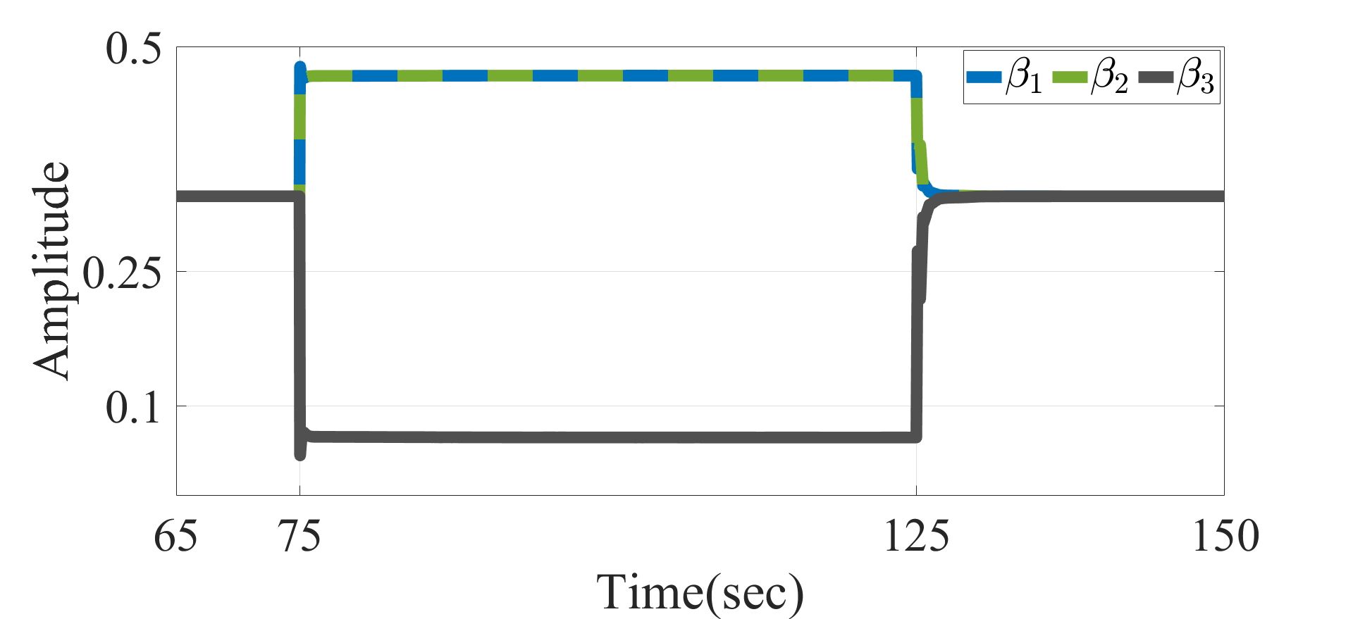
Figure 2: Automatic distribution of the control input among actuators

It shows that the faulty pitch actuator receives less control input in response to the fault. Figure. 3 shows the pitch actuators.

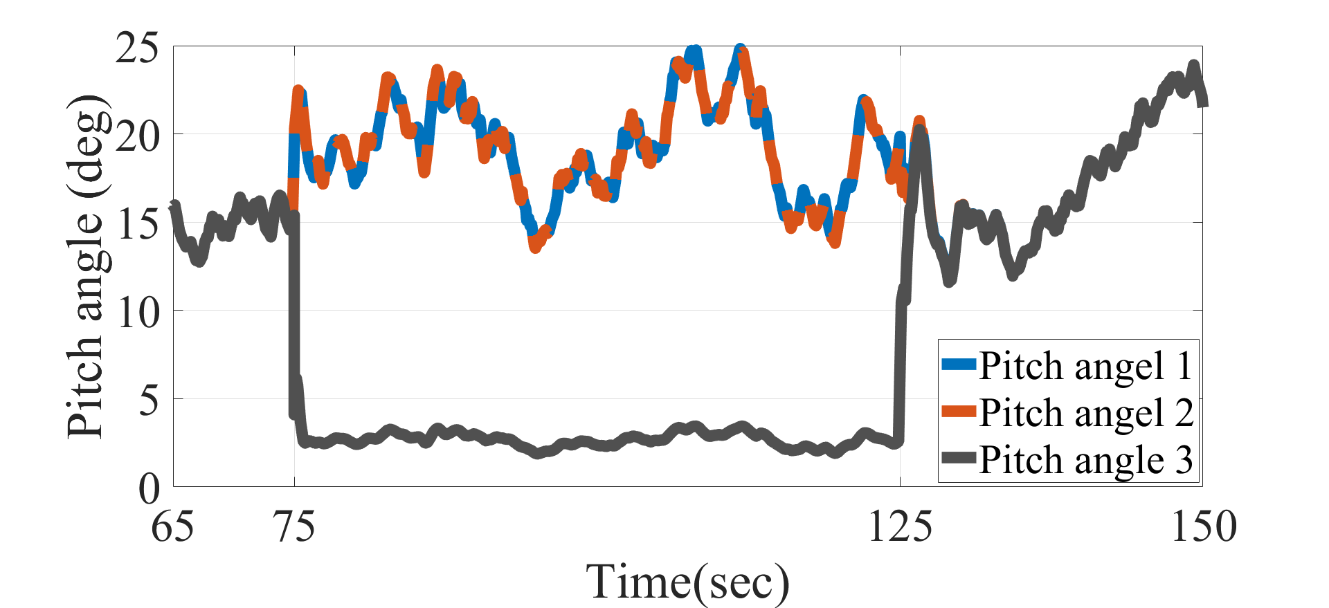
Figure 3: Pitch angle responses

Figure 4: Faulty pitch angle response

It shows that when the third actuator is faulty, the other two healthy actuators are collectively collaborating to compensate for the faulty actuator. Note that both healthy actuators have the same response due to the splitter design. The faulty pitch angles of the two controller are shown in Fig. 4. It shows that the adaptive SMC has huge spike at 125 sec when the fault vanishes abruptly. The reason is because the pitch actuators in the adaptive SMC does not collaborate collectively. The online parameter identification of the natural frequency is shown in Fig. 5.

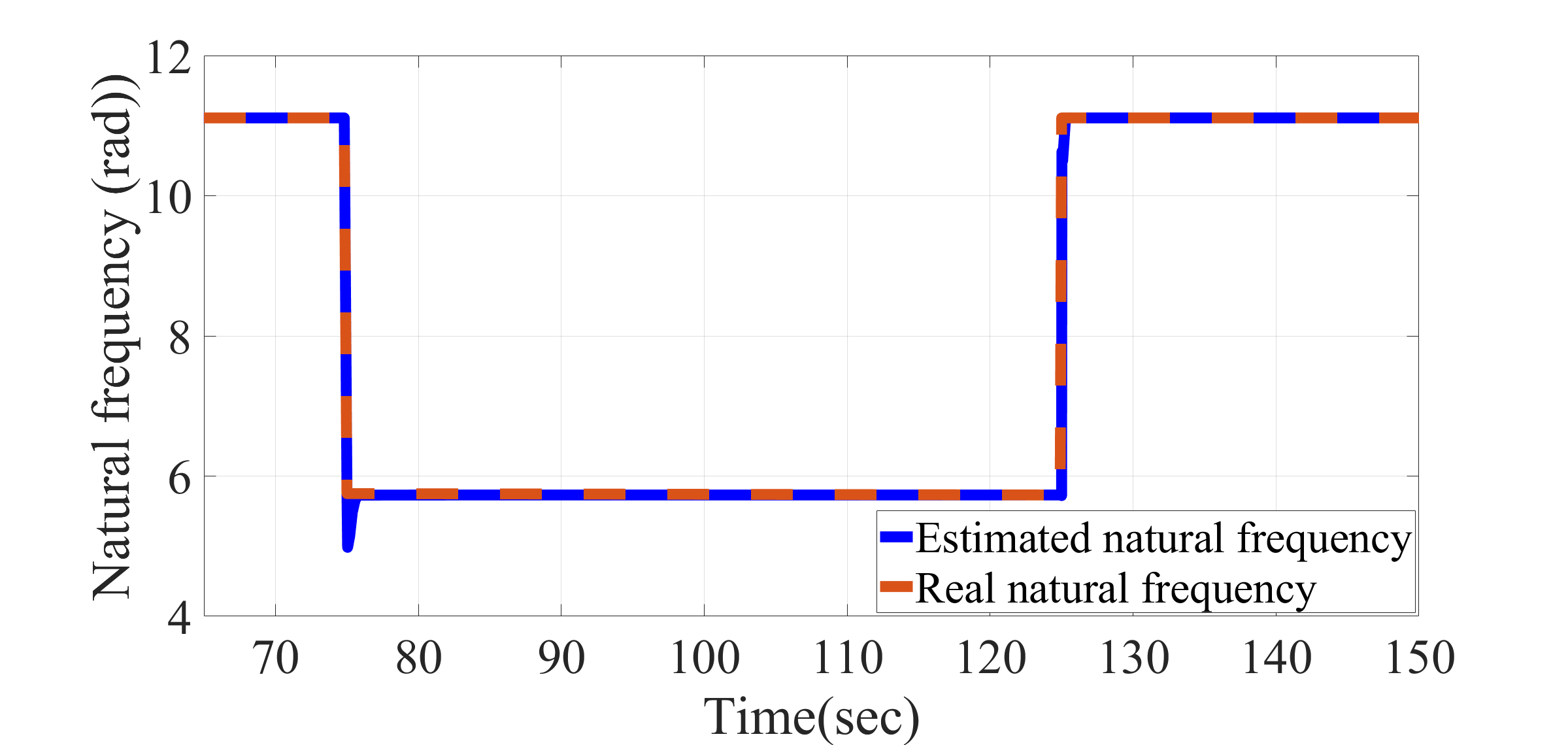
Figure 5: Online identification of the Natural frequency

It shows that the estimator is fast and precise in tracking the time-varying natural frequency. The rotor speed response is shown in Fig. 6, and Fig. 7. It shows that the proposed controller has less fluctuations especially it significantly outperforms the adaptive SMC when the fault occurs at 75 sec.

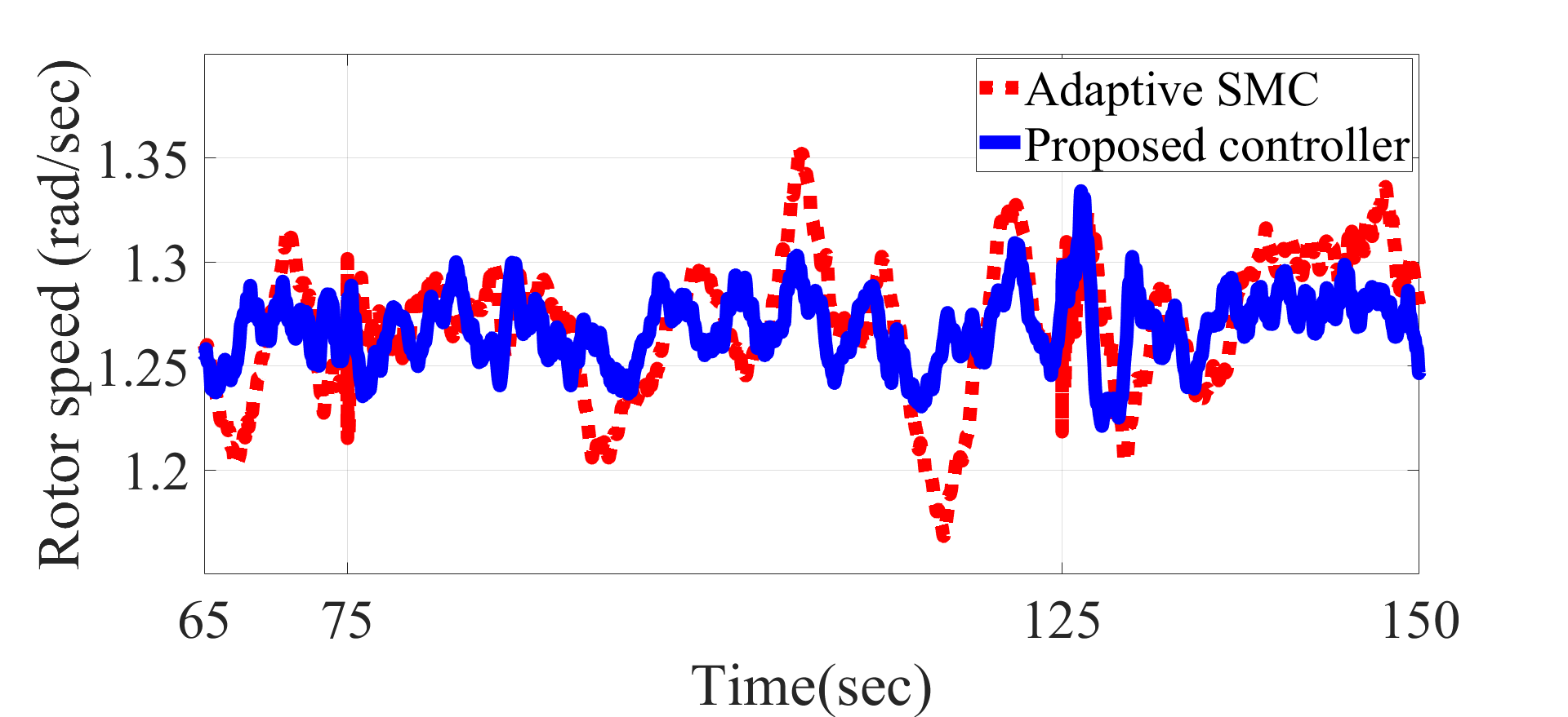
Figure 6: Rotor speed response

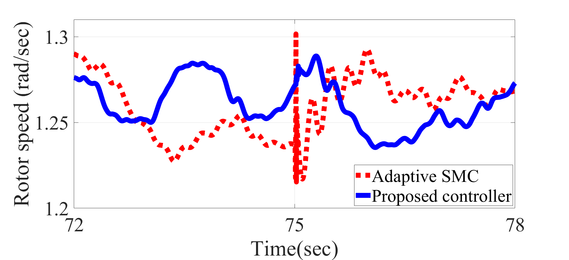
Figure 7: Rotor speed response

6 Conclusion

This paper addressed the problem for a class of nonlinearly coupled hierarchical systems including multi-agents subjected to actuator faults whose outputs should be collectively controlled. A splitter using parameter estimation along with a controller is proposed in response to the faults such that they collectively track a desired output required for the high-level dynamics. It was shown that the high-level closed-loop system is $\mathcal{L}_{2}$-gain-stable, while the error in the low-level is asymptotically stable. The results show that the splitter improves the transient response.

References

• Able (1956) Able, B. (1956). Nucleic acid content of microscope. Nature, 135, 7–9.
• Able et al. (1954) Able, B., Tagg, R., and Rush, M. (1954). Enzyme-catalyzed cellular transanimations. In A. Round (ed.), Advances in Enzymology, volume 2, 125–247. Academic Press, New York, 3rd edition.
• Keohane (1958) Keohane, R. (1958). Power and Interdependence: World Politics in Transitions. Little, Brown & Co., Boston.
• Powers (1985) Powers, T. (1985). Is there a way out? Harpers, 35–47.