Abstract

We present a novel mechanism which leads to the baryon asymmetry generation during the strong first order phase transition. If the bubble wall propagates with ultra-relativistic velocity, it has been shown [1] that it can produce states much heavier than the scale of the transition and that those states are then out of equilibrium. In this paper, we show that this production mechanism can also induce CP-violation at one-loop level. We calculate those CP violating effects during the heavy particle production and show, that combined with baryon number violating interactions, those can lead to successful baryogenesis. Two models based on this mechanism are constructed and their phenomenology is discussed. Stochastic gravitational wave signals turn out to be generic signatures of this type of models.

1 Introduction

One of the greatest puzzles of the early universe cosmology is the origin of the observed excess of matter over anti-matter. The over-abundance of matter is commonly parametrized via the baryon-to-photon density ratio

$$Y_{B}\equiv\frac{n_{B}-n_{\bar{B}}}{s}\bigg{|}_{0}$$ (1)

with $n_{B},n_{\bar{B}}$ and $s$ respectively the number density of baryons, anti-baryons and the entropy density. The subscript 0 means “at present time”. Planck data and evolution models of the early universe permit to compute this ratio with high accuracy[2]

$$Y_{B}=(8.75\pm 0.23)\times 10^{-11}.$$ (2)

Though this ratio is much smaller than unity, it calls for an explanation in terms of early universe dynamics, i.e. baryogenesis. The necessity of baryogenesis aggravates in the inflationary cosmology since this asymmetry ratio cannot be attributed to the initial conditions.

For a successful baryogenesis scenario, the well-known Sakharov requirements should be satisfied [3] namely the violation of the baryon number, violation of $C$ and $CP$ symmetries, and the presence of an out-of-equilibrium process. Based on this general requirements various models have been constructed (for reviews see for example [4, 5]) based on the different realizations of the Sakharov’s conditions. One interesting possibility for the fulfillment of the out-of-equilibrium process requirement is a scenario in which a first order phase transition (FOPT) occurs in the early history of the universe and this will be the focus of the study in the present paper. However in the standard model the phase transitions are not of the first order (neither QCD PT[6] nor electroweak one [7]). This fact prevents the realization, within the SM, of the very attractive idea of electroweak baryogenesis [8, 9]. This implies that physics beyond the standard model (BSM) is needed.

Various physically motivated extensions of the standard model, like MSSM or composite Higgs models, could provide room for baryogenesis during the electroweak phase transition (EWPT) [10, 11, 12, 13, 14] (see [15] for review) or some other phase transitions [16] in the early universe. Interestingly, in most of the cases, the successful generation of the baryon asymmetry requires the slow motion of the bubble walls ( though bubble velocity can be supersonic [17, 18, 19] or in the case of specific models even relativistic [20]. In this paper we propose a new mechanism for the production of the baryon asymmetry during the first order phase transition, which is only effective in the opposite regime i.e. for the ultra-relativistic bubble wall expansions. The idea will be based on the recent observation in [1] , where it was shown that in the presence of a ultra-relativistic bubble expansion, with Lorentz factor $\gamma_{w}\gg 1$, particles with mass up to $M\lesssim\sqrt{\gamma_{w}T_{\text{nuc}}\times v}$ can be produced. The parameters $T_{\text{nuc}}$ and $v$ are the temperature of FOPT (nucleation temperature) and the scale of the symmetry breaking respectively. The process of the heavy states production during the FOPT is obviously out-of-equilibrium, so that if it proceeds through a CP-violating and process and baryon number is not preserved we can have a successful baryogenesis scenarios. We confirm the statements above by analyzing the CP-violating effects in the interference of tree and one loop level processes. Then we construct explicit models where the baryogenesis is realized during the strong FOPT, which can be either the EWPT itself, if it comes with the necessary new physics, or related to some other symmetry breaking in the early universe.

One of the interesting feature of this class of models is that, contrary to the “traditional” baryogenesis models, it needs ultra-relativistic bubble wall velocities and is generically accompanied with strong gravitational waves signal.

The remaining of the paper is organized as follows: in the section 2, we review the mechanism of the heavy state production proposed in [1] and calculate the CP violation in this process. In the section 3 we build two models of baryogenesis and discuss their phenomenology and then in the section 4 we conclude by recapitulating the main results of this work.

2 Mechanism of CP-violation via bubble wall

2.1 Production of the heavy states in the phase transition

Let us start by reviewing the process of heavy states production during the phase transition presented in [1]. We will assume that the phase transition is of first order and that the bubbles reach ultra-relativistic velocities during the expansion $\gamma\gg 1$. We discuss the conditions for such a dynamics in Appendix A. To make the discussion explicit we assume the following Lagrangian:

$$\mathcal{L}=|\partial_{\mu}\phi|^{2}+i\bar{\chi}\mathord{\not\mathrel{{\mathrel{\partial}}}}\chi+i\bar{N}\mathord{\not\mathrel{{\mathrel{\partial}}}}N-M\bar{N}N-Y\phi\bar{N}\chi-V(\phi)$$ (3)

where $\phi$ is a scalar field undergoing a FOPT of e.g. global $U(1)$ symmetry, $\chi$ a light fermion and $N$ a heavy Dirac fermion with mass $M\gg\langle{\phi}\rangle$, $M\gg T_{\text{nuc}}$ and $Y$ is the coupling between the scalar and the two fermions. $V(\phi)$ is a potential for the field $\phi$, which we will assume leads to the FOPT without specification of its explicit form. Here and hereafter, without loss of generality, we work in the basis where fermion masses are real. So that before, during and after the FOPT the equilibrium abundance of $N$ is exponentially suppressed. However in the case of an ultra-relativistic bubble expansion, the probability that the light $\chi$ fluctuates via mixing to the heavy $N$ is non-vanishing [1] and is approximately equal to

$$\mathcal{P}^{tree}(\chi\to N)\approx\frac{Y^{2}\langle{\phi}\rangle^{2}}{M^{2}}\Theta(\gamma_{w}T_{\text{nuc}}-M^{2}L_{w})$$ (4)

with $L_{w}\sim 1/\langle{\phi}\rangle$ the length of the wall. Thus, when the ultra-relativistic wall hits the plasma, it produces $N$ and $\bar{N}$. Note that this abundance will be much larger than its equilibrium value.

2.1.1 Method of calculation of the light $\to$ heavy transition

Before we proceed to the one loop calculation, let us present a generic method to compute the transition amplitudes. We will then apply it to recover Eq.(4) and later for the computations of the one loop corrections. In this section we will omit the flavour indices which we will easily recover once the loop functions will be derived.

Let us look at the correlation function $\langle 0|T\{\bar{\chi}(x_{1})N(x_{2})\}|0\rangle$ and calculate it to first order in ${\cal O}\left(\frac{\langle{\phi}\rangle}{M}\right)$ which will be our expansion parameter. We assume that the wall is located in $x-y$ plane at $z=0$. The correlation functions writes

$$\langle 0|T\{\bar{\chi}(x_{1})N(x_{2})\}|0\rangle=\int d^{4}xY\langle{\phi(x)}\rangle S_{\chi}(x_{1}-x)S_{N}(x-x_{2})+\mathcal{O}\left(\frac{Y\langle{\phi}\rangle}{M}\right)^{2}$$ (5)

where we are expanding the correlation functions of the theory with $\langle{\phi}\rangle\neq 0$ in terms of the correlation functions $S_{\chi,N}$ of the unbroken $\langle{\phi}\rangle=0$ theory. Then performing the Fourier transformation we will obtain

$$\int d^{4}xd^{4}kd^{4}qe^{ik(x_{1}-x)+iq(x-x_{2})}S_{\chi}(k)S_{N}(q)Y\langle{\phi(x)}\rangle$$

$$=\int d^{4}kd^{4}qe^{ikx_{1}-iqx_{2}}S_{\chi}(k)S_{N}(q)\times\left[(2\pi)^{3}\delta^{(3)}(k-q)\int dze^{iz(k_{z}-q_{z})}Y\langle{\phi(z)}\rangle\right],$$

$$\delta^{(3)}(k-q)\equiv\delta^{(1)}(k_{0}-q_{0})\delta^{(1)}(k_{x}-q_{x})\delta^{(1)}(k_{y}-q_{y}).$$ (6)

Let us make a few comments regarding this expressions. The propagators $S_{\chi,N}$ have poles at, respectively $p^{2}=0,M^{2}$ and this, together with energy and $(x-y)$-momentum conservation, fixes the exchange of momentum $\Delta p_{z}$ from the plasma to the wall;

$$\Delta p_{z}=q_{z}-k_{z}=-k_{z}+\sqrt{k_{z}^{2}-M^{2}}\approx-\frac{M^{2}}{2k_{z}}.$$ (7)

Now we can use the LSZ reduction formula to relate the correlation function to the matrix element of the $\chi\to N$ transition and we find that

$$\langle N,q|\chi,k\rangle=\left[(2\pi)^{3}\delta^{(3)}(k-q)\int dze^{-iz\Delta p_{z}}\langle{\phi(z)}\rangle\right]\times\bar{u}_{N}(q)u_{\chi}(k)Y$$ (8)

which coincides with the result found in[1]. Note that the last factor is exactly equal to the amplitude of the transition $\chi(k)\to N(q)\phi(\Delta p_{z})$, ${\cal M}_{\chi(k)\to N(q)\phi(\Delta p_{z})}$. Thus we can write

$$\langle N,q|\chi,k\rangle=\left[(2\pi)^{3}\delta^{(3)}(k-q)\int dze^{-iz\Delta p_{z}}\langle{\phi(z)}\rangle\right]{\cal M}_{\chi(k)\to N(q)\phi(\Delta p_{z})}.$$ (9)

Of course on-shell $\phi$ cannot have the space-like momentum $\Delta p_{z}$ but since it is a scalar we can still formally define such an “amplitude”. These relations are the consequence of the following Ward identity which is satisfied if we are looking at the effects with just one VEV $\langle{\phi}\rangle$ insertion:

$$\langle O_{1}(x_{1})...O_{n}(x_{n})\phi(x_{n+1})\rangle|_{\langle{\phi}\rangle=0}=\int dz\left[\frac{\delta}{\delta\langle{\phi(z)}\rangle}\langle O_{1}(x_{1})...O_{n}(x_{n})\rangle|_{\langle{\phi}\rangle\neq 0}\right]D_{\phi}(x_{n+1}-z),$$ (10)

where $D_{\phi}$ is the propagator of the $\phi$ field. Then the application of the LSZ reduction together with energy and transverse momentum conservation leads to the Eq.(9).

2.1.2 Probability of the light $\to$ heavy transition

Armed with the generic expression in Eq. (9) we can proceed to the computation of the light $\to$ heavy transition probability similarly to the discussion in [1, 21],

$$P_{\chi\to N}=\int\frac{d^{3}q}{(2\pi)^{3}2q_{0}2k_{0}}(2\pi)^{3}\delta^{(3)}(k-q)|{\cal M}_{\chi(k)\to N(q)\phi(\Delta p_{z})}|^{2}\left|\int dze^{-iz\Delta p_{z}}\langle{\phi(z)}\rangle\right|^{2}.$$ (11)

Performing the phase space integral and summing (averaging) over incoming (outgoing) spins, we arrive at

$$P_{\chi\to N}=\left|\int dze^{-iz\Delta p_{z}}\langle{\phi(z)}\rangle\right|^{2}\times\frac{|Y|^{2}k_{z}(k_{z}-\sqrt{k_{z}^{2}-M^{2}})}{2k_{0}\sqrt{k_{z}^{2}-M^{2}}}$$ (12)

Let us evaluate the first prefactor which takes into account the shape of the wall. To approximate the integral, we need to use some estimation for the shape of the wall. For example for a linear wall ansatz of the form

$$\langle\phi(z)\rangle=\left\{\begin{array}[]{c}0,~{}~{}z<0\\ \langle\phi\rangle\frac{z}{L_{w}}~{}~{}~{}0\leq z\leq L_{w}\\ \langle\phi\rangle~{}~{}~{}z>L_{w}\end{array}\right.$$ (16)

(where we use $\langle\phi\rangle$ as the VEV of $\phi$ in the true vacuum) we obtain

$$\left|\int dze^{-iz\Delta p_{z}}\langle{\phi(z)}\rangle\right|^{2} = \frac{\langle{\phi}\rangle^{2}}{\Delta p_{z}^{2}}\bigg{(}\frac{\sin\alpha}{\alpha}\bigg{)}^{2},\qquad\alpha=\frac{L_{w}\Delta p_{z}}{2}.$$ (17)

We thus observe the appearance of a new suppression factor that becomes relevant in the limit $\alpha=\frac{L_{w}\Delta p_{z}}{2}\gg 1$ and quickly suppresses the transition. Similar results holds for more realistic wall shapes when it is given by either $\tanh$ or gaussian functions

$$\langle\phi\rangle_{\text{tanh}}(z)=\frac{\langle{\phi}\rangle}{2}\bigg{[}\tanh{\left(\frac{z}{L_{w}}\right)}+1\bigg{]},\qquad\langle\phi\rangle_{\text{gaussian}}(z)=\frac{\langle{\phi}\rangle}{\sqrt{2\pi}L_{w}}\int_{-\infty}^{z}dz^{\prime}\exp{\left(-\frac{z^{\prime 2}}{2L_{w}^{2}}\right)}.$$ (18)

In these cases we find respectively (see for details of calculation [21]):

$$\left|\int dze^{-iz\Delta p_{z}}\langle{\phi(z)}\rangle\right|^{2}_{\text{tanh}} = \left[\frac{\pi L_{w}}{2\sinh{\left(\frac{L_{w}\Delta p_{z}\pi}{2}\right)}}\right]^{2}\langle{\phi}\rangle^{2},$$

$$\left|\int dze^{-iz\Delta p_{z}}\langle{\phi(z)}\rangle\right|^{2}_{\text{gaussian}} = \frac{\langle{\phi}\rangle^{2}}{\Delta p_{z}^{2}}\exp{\left(-L_{w}^{2}\Delta p_{z}^{2}\right)}.$$ (19)

Thus we can see that independently of the wall shape the transitions with $\Delta p_{z}\gg L_{w}^{-1}$ are strongly suppressed. In the opposite regime $\Delta p_{z}\lesssim L_{w}^{-1}\sim\langle{\phi}\rangle$ we will have $k_{z}\gtrsim M^{2}/\langle{\phi}\rangle$. Then expanding the Eq. (12), we will obtain

$$P_{\chi\to N}\simeq\frac{Y^{2}\langle{\phi}\rangle^{2}}{M^{2}}\Theta(k_{0}-M^{2}L_{w}),$$ (20)

which reduces to Eq.(4) when we notice that $k_{0}\sim\gamma_{w}T_{\rm nuc}$. We can see that indeed there will be an efficient production of the heavy states, which will not be Boltzmann suppressed, however the Lorentz boost factor $\gamma_{w}$ for the wall expansion needs to be large enough.

After this warm-up exercise we can proceed to the calculation of the one loop effects. We will focus again only on the terms with just one VEV $\langle{\phi}\rangle$ insertion and proceed in the same way as we have done for the tree level calculation. Note that the Eq. (9) will remain true also at loop level if we are focusing only on the effects with one VEV insertion. Indeed the momentum is not conserved only in the vertex with the $\langle{\phi}\rangle$ insertion, however the energy and $x-y$ momentum conservation still fixes the value of the loss of the $z$ component of momentum. At this point since $\phi$ is a scalar (no polarization vectors are needed) the matrix element is exactly the same as for the process $\chi(k)\to N(q)\phi(\Delta p_{z})$ and can be calculated using the usual Lorentz invariant Feynman diagram techniques.

2.2 CP violation in production

So far we have been looking at $\chi\to N$ transition. However if there are more than one species of $\chi,N$ then the couplings $Y$ become in general complex matrices, and, if it contains a physical phase, this can lead to CP violating processes. The Lagrangian (3) generalises to

$$\mathcal{L}=i\bar{\chi}_{i}P_{R}\mathord{\not\mathrel{{\mathrel{\partial}}}}\chi_{i}+i\bar{N}_{I}\mathord{\not\mathrel{{\mathrel{\partial}}}}N_{I}-M_{I}\bar{N}_{I}N_{I}-Y_{iI}\phi\bar{N}_{I}P_{R}\chi_{i}-y_{I\alpha}(h\bar{l}_{\alpha})P_{R}N_{I}+h.c.$$ (21)

where $h$ and $l_{\alpha}$ are the usual SM Higgs and fermions that we couple to the heavy $N_{I}$, $P_{R},P_{L}$ are the chiral projectors. We choose this assignment of chirality in agreement with our further toy models. In particular the rates $\Gamma(\chi_{i}\to N_{I})\neq\Gamma(\bar{\chi}_{i}\to\bar{N}_{I})$ and after the phase transition there could be an asymmetry in $N,\bar{N}$ and $\chi,\bar{\chi}$ populations. Let us calculate these asymmetries. It is known that at tree level no asymmetries can be generated since both processes will be proportional to $|Y_{iI}|^{2}$, so we need to consider one loop corrections to it, in particular it is known that the imaginary part of the loop is the crucial ingredient for asymmetry generation. In general performing such calculation in the presence of the bubble wall background is quite involved, however things simplify if the bubble expansion is ultra-relativistic. Then we can expand in $\frac{\langle{\phi}\rangle}{E}\sim\frac{\langle{\phi}\rangle}{\gamma T}$ parameter. In this case it will be sufficient, similarly to the tree level result, to focus only on the effects in the matrix element at ${\cal O}\left(\frac{\langle{\phi}\rangle}{\gamma T}\right)$ i.e. one scalar VEV insertion.

2.2.1 Calculation of the light $\to$ heavy transition at 1-loop level

Let us now compute the asymmetries in the populations of the various particle immediately after the PT in the case of the model in Eq.(21). First of all we need to know the CP violating effects in the $\chi_{i}\to N_{I}$ transition, which will appear in the interference of the loop and tree level diagrams.

$$A(\chi_{i}\to N_{I})_{\rm tree}\propto Y_{iI}$$

$$A(\chi_{i}\to N_{I})_{\rm 1-loop}\propto\sum_{k,J}Y_{iJ}Y_{kJ}^{*}Y_{kI}\times f^{(\chi\phi)}_{IJ}+\sum_{\alpha,J}Y_{iJ}y_{\alpha J}^{*}y_{\alpha I}\times f^{(hl)}_{IJ}$$ (22)

where the functions $f^{(hl)}$ and $f^{(\chi\phi)}$ refer to the loop diagrams with virtual $\chi,\phi$ and $hl$ respectively. As a consequence, there will be the following asymmetries in $N_{I}$ populations immediately after the PT

$$\epsilon_{Ii}\equiv\frac{|\mathcal{M}_{i\to I}|^{2}-|\mathcal{M}_{\bar{i}\to\bar{I}}|^{2}}{\sum_{i}|\mathcal{M}_{i\to I}|^{2}+|\mathcal{M}_{\bar{i}\to\bar{I}}|^{2}}$$

(23)

$$=\frac{2\sum_{k,J}{\rm Im}(Y_{iI}Y_{iJ}^{*}Y_{kJ}Y^{*}_{kI}){\rm Im}f^{(\chi\phi)}_{IJ}}{\sum_{i}|Y_{iI}|^{2}}+\frac{2\sum_{\alpha,J}{\rm Im}(Y_{iI}Y_{iJ}^{*}y_{\alpha J}y^{*}_{\alpha I}){\rm Im}f^{(hl)}_{IJ}}{\sum_{i}|Y_{iI}|^{2}},$$ (24)

where $\epsilon_{Ii}$ refers to asymmetry in $N_{I}$ particle population which are produced from the $i$ initial flavour of $\chi_{i}$. The loop functions take the form

$$f^{(hl)}_{IJ}(x)\equiv 2\int\frac{d^{4}p}{(2\pi)^{4}}\frac{P_{R}\not{p}P_{L}(\not{p}_{out}+M_{J})P_{L}}{(p^{2}+i\epsilon)((p-p_{out})^{2}+i\epsilon)(p_{out}^{2}-M_{I}^{2}+i\epsilon)}$$ (25)

$$f^{(\chi\phi)}_{IJ}(x)\equiv\int\frac{d^{4}p}{(2\pi)^{4}}\frac{P_{L}\not{p}P_{R}(\not{p}_{out}+M_{J})P_{L}}{(p^{2}+i\epsilon)((p-p_{out})^{2}+i\epsilon)(p_{out}^{2}-M_{I}^{2}+i\epsilon)},$$ (26)

where $p,p_{out}$ are the initial (particle $i$) and final (particle $I$) state four momenta. The factor of two in front of the $f^{(hl)}_{IJ}(x)$ function comes from the two contributions with a loop of $\nu_{L},h^{0}$ and $e_{L},h^{+}$. This factor is absent in the case of $f^{(\chi\phi)}_{IJ}(x)$ because we have only the loop of $\chi,\phi$. The imaginary part of those loop functions take the form

$$\text{Im}[f^{(hl)}_{IJ}(x)]=\frac{1}{16\pi}\frac{\sqrt{x}}{1-x},\qquad x=\frac{M_{J}^{2}}{M_{I}^{2}}$$ (27)

$$\text{Im}[f^{(\chi\phi)}_{IJ}(x)]=\frac{1}{32\pi}\frac{1}{1-x}.$$ (28)

Summing over the flavours of $\chi_{i}$ we arrive at the following asymmetry in $N_{I}$ abundance

$$\epsilon_{I}\equiv\sum_{i}\epsilon_{Ii}=\frac{2\sum_{\alpha,J,i}{\rm Im}(Y_{iI}Y_{iJ}^{*}y_{\alpha J}y^{*}_{\alpha I}){\rm Im}f^{(hl)}_{IJ}}{\sum_{i}|Y_{iI}|^{2}}.$$ (29)

Note that the only diagrams contributing to the asymmetry are shown on the Fig.1) and these have virtual $hl$.

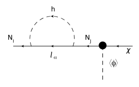
Figure 1: The diagram contributing to the function $f^{(hl)}$

So far we have shown that during the production we can create a difference in the abundances of $N_{I}$ and $\bar{N}_{I}$ inside the bubble. However since it was produced by $1\to 1$ transitions exactly the same difference will be present inside the bubble also for the abundances of $\bar{\chi}_{i}$ and $\chi_{i}$. Using the “$\langle{\phi}\rangle\neq 0$” and “$\langle{\phi}\rangle=0$” subscribes for the particle densities inside and outside the bubbles and taking into account that the number density of some particle entering inside the bubble is $n=\frac{\Delta N}{\Delta A\Delta t}\frac{\Delta t}{\Delta z}=\frac{J}{v_{w}}$ with entering flux $J=\int\frac{p_{z}d^{3}p}{p_{0}(2\pi)^{3}}f_{\chi}(p,T_{\text{nuc}})$ we can conclude that, in the plasma frame,

$$n_{N_{I}}^{\langle{\phi}\rangle=0}(T_{\text{nuc}})\simeq 0,\hbox{~{}~{}~{}~{}Boltzmann suppressed}$$ (30)

and

$$n_{N_{I}}^{\langle{\phi}\rangle\neq 0} \simeq \frac{1}{\gamma_{w}v_{w}}\int\frac{d^{3}p}{(2\pi)^{3}}P_{\chi\to N}(p)\times f_{\chi}(p,T_{\text{nuc}})$$ (31)

$$\simeq \sum_{i}\frac{|Y_{iI}|^{2}\langle{\phi}\rangle^{2}}{M_{I}^{2}\gamma_{w}v_{w}}\int\frac{d^{3}p}{(2\pi)^{3}}\times f^{eq}_{\chi}(p,T_{\text{nuc}})\Theta(p_{z}-M_{I}^{2}/\langle{\phi}\rangle)$$

$$\simeq \sum_{i}\frac{|Y_{iI}|^{2}}{\pi^{2}\gamma_{w}^{3}v_{w}}\times\frac{\langle{\phi}\rangle^{2}T_{\text{nuc}}^{2}}{M_{I}^{2}}\bigg{(}\frac{M_{I}^{2}/\langle{\phi}\rangle}{1-v_{w}}+\frac{T_{\text{nuc}}(2-v_{w})}{\gamma_{w}(v_{w}-1)^{2}}\bigg{)}\times e^{-\gamma_{w}\frac{M_{I}^{2}}{\langle{\phi}\rangle}\frac{1-v_{w}}{T_{\text{nuc}}}}$$

$$= \sum_{i}\frac{|Y_{iI}|^{2}T_{\text{nuc}}^{3}\langle{\phi}\rangle^{2}}{\pi^{2}M_{I}^{2}}e^{-\frac{M_{I}^{2}}{2\langle{\phi}\rangle T_{\text{nuc}}\gamma_{w}}}+\mathcal{O}(1/\gamma_{w})$$

$$\simeq \sum_{i}\theta_{iI}^{2}n_{\chi^{i}}^{\langle{\phi}\rangle=0}(T_{\text{nuc}}).$$

where $v_{w}=\sqrt{1-1/\gamma_{w}^{2}}\approx 1-\frac{1}{2\gamma_{w}^{2}}$ is the velocity of the wall. The integral is performed in the wall frame and the $\gamma_{w}^{-1}$ factor in front takes care of the conversion to the plasma frame. In the second line we introduced the expression Eq.(20) of the probability of light to heavy transition and assumed that, the transition being a detonation, the density distribution of $\chi$ is the equilibrium distribution $f^{eq}_{\chi}\approx e^{-\frac{{\gamma_{w}}(E_{\chi}-v_{w}p^{\chi}_{z})}{T_{\text{nuc}}}}$ (using Boltzmann distribution as a simplifying assumption) and $E_{\chi}=\sqrt{p_{z}^{2}+\vec{p}^{2}_{\perp}}$. In the third line we performed the phase space integral. In the last approximation, we have taken the exponential to be unity since the wall is relativistic and $\gamma_{w}T_{\rm nuc}\gg M_{I}$, and defined

$$\theta_{iI}\equiv\frac{|Y_{iI}|\langle{\phi}\rangle}{M_{I}}.$$ (32)

This means that some of the abundance of $\chi_{i}$ has been removed from the plasma and since we are focusing on $1\to 1$ transitions, this gives :

$$\sum_{I}\Delta n_{N^{I}}=-\sum_{i}\Delta n_{\chi^{i}}\Rightarrow$$

$$\sum_{I}\left(\Delta n_{N^{I}}-\Delta n_{\bar{N}^{I}}\right)=-\sum_{i}\left(\Delta n_{\chi^{i}}-\Delta n_{\bar{\chi}^{i}}\right),$$ (33)

where $\Delta n_{N,\chi}$ are the differences in abundances of the particles in the broken and unbroken phases. As a consequence, there will be also an asymmetry in the abundances of the light fields. Note that the asymmetry in the $\chi$ field will be further diluted by the factor $\sim\frac{y^{2}\langle{\phi}\rangle^{2}}{M^{2}}$ due to the large symmetric thermal densities of the light fields during and after the phase transition.

	$N_{I}$	$N_{I}^{c}$	$\chi_{i}$	$\chi_{i}^{c}$	$\Delta n_{N^{I}}$
$\epsilon=0$, without CP-violation
Out	0	0	$n_{\chi^{i}}$	$n_{\chi^{i}}$	0
In	$\theta^{2}_{Ii}n_{\chi^{i}}$	$\theta^{2}_{Ii}n_{\chi^{i}}$	$(1-\theta^{2}_{Ii})n_{\chi^{i}}$	$(1-\theta^{2}_{Ii})n_{\chi^{i}}$	0
$\epsilon\neq 0$, with CP-violation
Out	0	0	$n_{\chi^{i}}$	$n_{\chi^{i}}$	0
In	$\theta^{2}_{Ii}(1-\epsilon_{Ii})n_{\chi^{i}}$	$\theta^{2}_{Ii}(1+\epsilon_{Ii})n_{\chi^{i}}$	$(1-\theta^{2}_{Ii}(1-\epsilon_{Ii}))n_{\chi^{i}}$	$(1-\theta^{2}_{Ii}(1+\epsilon_{Ii}))n_{\chi^{i}}$	$2\epsilon_{Ii}\theta^{2}_{Ii}n_{\chi^{i}}$

Table 1: Densities and asymmetry, with and without CP-violation, inside and outside of the bubble. For clarity we got rid of the temperature dependence, assuming that the density have to be evaluated at the nucleation temperature.

3 Application of the mechanism for baryogenesis

In the previous section we have shown that the wall, if it becomes relativistic enough, can produce states much heavier than the reheating temperature and also that this production process can induce CP-violation via the interference of tree-level and loop-level diagrams.

Now we will present some examples of applications of this new CP-violating source for the explanation of the observed matter asymmetry. Of course, many other examples could take advantage of the configuration presented in the previous section, so what we will present now serve as a proof of existence. For this reason, in the following we will present two classes of models that take advantage of the mechanism present above.

3.1 Phase-transition induced leptogenesis

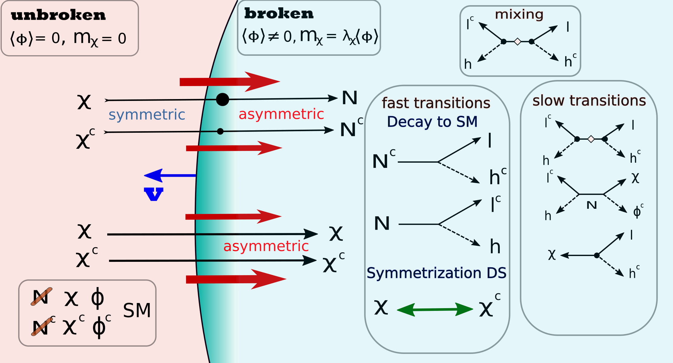
Figure 2: Mechanism at play in the phase transition-induced leptogenesis. In the diagrams the black dot denotes a mixing between $\chi$ and $N$ and so the insertion of a factor of $\theta$, the white diamond is a $\chi$ mixing insertion. A thicker arrow designates a larger flux (though it is exaggerated on the figure.)

Let us consider the following extension of the Lagrangian in Eq.21, where we have introduced $\phi$ -dependent Majorana mass for the field $\chi$ and kept the rest of the interactions the same. We restrict to only one specie of the Majorana fermion $\chi$, since it is sufficient for the generation of CP phase.

$$\mathcal{L}_{\text{int}} = \underbrace{\sum_{I}\bigg{(}Y_{I}(\phi^{\dagger}\bar{\chi})P_{L}N_{I}+Y_{I}^{\star}\bar{N}_{I}P_{R}(\phi\chi)\bigg{)}-V(\phi)+\frac{1}{2}\lambda_{\chi}\phi\bar{\chi}^{c}\chi+\sum_{I}M_{I}\bar{N}_{I}N_{I}}_{\text{Toy model of Dark Sector}}$$

$$+ \underbrace{\sum_{\alpha I}y_{\alpha I}(h\bar{l}_{\alpha,SM})P_{R}N_{I}+h.c.}_{\text{Connection to SM}},$$

The interactions in Eq. 3.1 respect $U(1)$ lepton number with the following charge assignments $L(\chi)=-1,L(N)=1$ and $L(\phi)=2$. This symmetry is obviously broken after the phase transition by the VEV of $\langle{\phi}\rangle$ field and the Majorana mass of the $\chi$ field $m_{\chi}=\lambda_{\chi}\langle{\phi}\rangle$. Perturbativity bound imposes that $\lambda_{\chi}\lesssim\sqrt{4\pi}$. This model is only an example of the realisation of our scenario, we list some alternatives in Appendix B. The generation of the baryon asymmetry proceeds as follows: during the bubble expansion we generate asymmetry in $N$ and $\chi$, as they have been estimated in the section 2.2.1. Immediately after the transition, the asymmetry in $\chi$ is washed out due to the lepton-number violating Majorana mass term, which constitutes the first source of asymmetry for the system. Part of this asymmetry in $N$ is passed to the SM lepton sector during the decay $N\to lh$, which constitutes a second source of asymmetry for the system, via the usual CP-violating decay. We will see that the dominant contribution depends on the different couplings of the systems. This asymmetry in return is passed to the baryons by sphalerons, similarly to the original leptogenesis models [35]. The scheme of the construction is shown on the Fig.2.

3.1.1 Estimating the baryon asymmetry

So far we have generated the asymmetry in $N$ particle population, however we need to find what part of it will be passed to SM lepton sector. This can be done by comparing the branching ratios of $N\to hl$ and $N\to\chi\phi$ decays

$$\frac{n_{l}-n_{l^{c}}}{s} \simeq \frac{1}{s(T_{reh})}\sum_{iI}\epsilon_{Ii}\frac{3\zeta(3)|Y_{iI}|^{2}T_{\text{nuc}}^{3}\langle{\phi}\rangle^{2}}{4\pi^{2}M_{I}^{2}}\times\frac{Br(N_{I}\to hl)}{Br(N_{I}\to hl)+Br(N_{I}\to\chi\phi)}$$

$$\simeq \frac{135\zeta(3)g_{\chi}}{8\pi^{4}g_{\star}}\sum_{I}\theta^{2}_{I}\frac{2\sum_{\alpha,J}{\rm Im}(Y_{I}Y_{J}^{*}y_{\alpha J}y^{*}_{\alpha I}){\rm Im}f^{(hl)}_{IJ}}{|Y_{I}|^{2}}\bigg{(}\frac{T_{nuc}}{T_{reh}}\bigg{)}^{3}\times{\frac{\sum_{\alpha}|y_{\alpha I}|^{2}}{\sum_{\alpha}|y_{\alpha I}|^{2}+{|Y_{I}|^{2}}}}$$

where $g_{*}$ is total number of degrees of freedom and $s(T)=\frac{2\pi^{2}}{45}g_{\star}T^{3}$, and $g_{\chi}$ is the number of degrees of freedom of $\chi$ particle. The reheating temperature, $T_{reh}$, is the temperature of the plasma immediately after the end of the transition, when the latent heat of the transition warmed up the plasma. If the transition is instantaneous, we can estimate $\frac{\pi^{2}g_{\star}[T_{\rm reh}]}{30}T_{\rm reh}^{4}=V[0]-V[v]+\frac{\pi^{2}g_{\star}[T_{\rm nuc}]}{30}T_{\rm nuc}^{4}$ where $V$ should be understood as the thermally corrected potential at the transition. By assuming $O(1)$ parameters in the potential and dominant latent heat, $T_{\rm reh}\sim v.$ The factor $\theta_{I}^{2}$ is the suppression due to the heavy field production and $\left(\frac{T_{\rm nuc}}{T_{reh}}\right)^{3}$ factor come from the fact that $n_{N}$ is fixed by the nucleation temperature (see Eq.(31)) and $s$ is at the reheating temperature after the PT. The factor ${\frac{\sum_{\alpha}|y_{\alpha I}|^{2}}{\sum_{\alpha}|y_{\alpha I}|^{2}+{|Y_{I}|^{2}}}}$ appears since a part of the asymmetry in $N$ is decaying back to $\phi\chi$, thus washing out a part of the asymmetry.

Lepton asymmetry generation in decay

Note that there is an additional effect contributing to the baryon asymmetry generation. The decays of the heavy fields $N$ are out of equilibrium and there is a CP phase in the Yukawa interactions. Thus the rates

$$\Gamma(N\to\bar{h}l)\neq\Gamma(\bar{N}\to h\bar{l})$$ (36)

induce a non-vanishing CP-violation in decay

$$\epsilon^{I}_{decay}\equiv\frac{\Gamma(N^{I}\to\bar{h}l)-\Gamma(\bar{N}^{I}\to h\bar{l})}{\Gamma(N^{I}\to\bar{h}l)+\Gamma(\bar{N}^{I}\to h\bar{l})}.$$ (37)

As a consequence, after the asymmetry induced by the production of heavy states, there will be an additional asymmetry due to the decay scaling as :

$$\left.\frac{n_{l}-n_{l^{c}}}{s}\right|_{decay}\sim\sum_{I}\frac{\theta^{2}_{I}}{g_{\star}}\epsilon_{decay}^{I}\bigg{(}\frac{T_{nuc}}{T_{reh}}\bigg{)}^{3}\times{\frac{\sum_{\alpha}|y_{\alpha I}|^{2}}{\sum_{\alpha}|y_{\alpha I}|^{2}+{|Y_{I}|^{2}}}}$$ (38)

where the asymmetry in decay $\epsilon^{I}$ will be generated by the diagram similar to the one in Fig.1 with $h,l$ in the final state and $\phi,\chi$ inside the loop. In the limit $m_{\chi},m_{\phi}\ll M_{I}$ (which is exactly where one VEV insertion approximation used in the section 2 is motivated) the loop function for both production and decay will be exactly the same up to the factor of 2 (particles running in the loop are EW singlets) compared to Eq.(29). However the couplings will be complex conjugates so that

$$\epsilon^{I}_{decay}=-\frac{{\rm Im}[Y_{I}Y^{*}_{J}y_{\alpha_{J}}y^{*}_{\alpha_{I}}]{\rm Im}[f^{(hl)}_{IJ}]}{\sum_{\alpha}|y_{\alpha I}|^{2}}.$$ (39)

Combining both effects and taking into account sphaleron rates converting the lepton asymmetry to the baryon, we obtain the following baryon asymmetry:

$$\frac{\Delta n_{B}}{s}\equiv\frac{n_{B}-n_{\bar{B}}}{s}\simeq -\frac{28}{79}\times\frac{135\zeta(3)g_{\chi}}{8\pi^{4}g_{*}}\times\sum_{I}{\theta^{2}_{I}}\sum_{\alpha,J}{\rm Im}(Y_{I}Y_{J}^{*}y_{\alpha J}y^{*}_{\alpha I}){\rm Im}f^{(hl)}_{IJ}$$ (40)

$$\times\left(\frac{2}{|Y_{I}|^{2}}-\frac{1}{\sum_{\alpha}|y_{\alpha I}|^{2}}\right)\bigg{(}\frac{T_{nuc}}{T_{reh}}\bigg{)}^{3}{\frac{\sum_{\alpha}|y_{\alpha I}|^{2}}{\sum_{\alpha}|y_{\alpha I}|^{2}+{|Y_{I}|^{2}}}}$$

The prefactor $-\frac{28}{79}$ comes from the sphalerons rates (see [36]). The observed asymmetry is given by $\frac{\Delta n_{B}}{s}\sim 8.8\times 10^{-11}$. The quantities in Eq.(40) can be estimated in the following way; outside of the resonance regime but for mild hierarchy between the masses of the heavy neutrinos $M_{1}\lesssim M_{2}\lesssim M_{3}$, $2{\rm Im}f^{(hl)}_{IJ}\to\frac{1}{8\pi}$, $g_{\star}\sim 100$ and ${\sum_{\alpha}|y_{\alpha I}|^{2}\gtrsim|Y_{I}|^{2}}$ induces ${\frac{\sum_{\alpha}|y_{\alpha I}|^{2}}{\sum_{\alpha}|y_{\alpha I}|^{2}+{|Y_{I}|^{2}}}}\sim 1$. As a consequence, the production of the observed asymmetry demands, in order of magnitude,

$$\text{Max}[\theta^{2}y^{2}]\bigg{(}\frac{T_{nuc}}{T_{reh}}\bigg{)}^{3}\sim 10^{-6}.$$ (41)

with an $O(1)$ CP phase and $|Y_{I}|\sim|Y_{J}|$.

3.1.2 Constraints on the model

Let us examine various bounds on the construction proposed. Let us start from neutrino masses. Indeed after the PT, the Lagrangian (3.1) generates a dimension 5 operator of the see-saw form [37, 38, 39, 40, 41]

$$\sum_{I,\alpha,\beta}\theta_{I}^{2}\frac{y_{\alpha I}y^{*}_{\beta I}(\bar{l}^{c}_{\alpha}h)(l_{\beta}h)}{m_{\chi}}$$ (42)

which induces a mass for the active neutrinos (for the heaviest light neutrino)

$$\text{Max}[m_{\nu}]\sim\text{Max}\bigg{[}\sum_{I}|y_{\alpha I}|^{2}\theta^{2}_{I}\bigg{]}\frac{v_{EW}^{2}}{m_{\chi}}.$$ (43)

Combining Eqs. (40), (43) with observed neutrino mass scale and the constraints $\text{Max}[\theta^{2}_{I}]\gtrsim 10^{-5},y\sim\mathcal{O}(1)$, we obtain the following constraints

$$\Rightarrow\qquad m_{\chi}\gtrsim 5\times 10^{9}\text{GeV}\qquad\Rightarrow\qquad\langle{\phi}\rangle\gtrsim 10^{9}\text{GeV}.$$ (44)

Let us list additional conditions on this baryogenesis scenario which must be satisfied. First of all, the decay processes of $\chi\to hl$, and $\chi\to(hl)^{*}$ have the same probability since $\chi$ is a Majorana fermion. Then we need to make sure that, immediately after the reheating, processes involving $\chi$ do not erase the asymmetry stored in the SM sector. Let us list these processes and their rates:

• $\chi$ production in $lh$ collisions: Ideally we have to solve the Boltzmann equation for the density evolution, which focusing only on this process will be given by:

  $$szH(z)\frac{dY_{l,l^{c}}}{dz}=-\frac{Y_{l,l^{c}}Y_{h}}{Y^{eq}_{l,l^{c}}Y^{eq}_{h}}\gamma(hl\to\chi)+\frac{Y_{\chi}}{Y_{\chi}^{eq}}\gamma(\chi\to lh,(l^{c}h)),$$ (45)

  where $z\equiv m_{\chi}/T$ (not to be confused with the spatial direction z along the wall) and $Y_{i}\equiv n_{i}/s$. However note that $\chi,\chi^{c}$ decay quickly with the rate $\Gamma\sim\frac{y^{2}\theta^{2}m_{\chi}}{4\pi}\gg H$ unless we consider the scales close to the Planck mass, this process induces that the density $Y_{\chi}$ is always kept close to equilibrium. Introducing the asymmetry density $Y_{\Delta_{\alpha}}\equiv Y_{l_{\alpha}}-Y_{l_{\alpha}^{c}}$ and subtracting for the matter anti-matter densities, we obtain

  $$szH(z)\frac{dY_{\Delta_{\alpha}}}{dz}=-\frac{Y_{\Delta_{\alpha}}}{Y_{l_{\alpha}}}\gamma(hl_{\alpha}\to\chi)$$ (46)

  where $\gamma_{\alpha}[z]\equiv\gamma(hl_{\alpha}\to\chi)$ is given by[42]

  $$\gamma_{\alpha}[z]=\frac{g_{\chi}T^{3}}{2\pi^{2}}z^{2}K_{1}(z)\Gamma_{\alpha}$$ (47)

  where the Bessel functions $K_{1}(z)$ satisfy the two limiting behaviours

  $$zK_{1}(z)=\begin{cases}1\qquad z\ll 1,\\ \sqrt{\frac{\pi z}{2}}e^{-z}\qquad z\gg 1.\end{cases}$$ (48)

  So, for large values of $z$, we get

  $$\frac{dY_{\Delta_{\alpha}}}{dz}\simeq-\frac{0.42e^{-z}z^{5/2}}{g_{*}^{1/2}g_{\alpha}}\left(\frac{M_{p}}{m_{\chi}}\right)\left(\frac{g_{\chi}\Gamma_{\alpha}}{m_{\chi}}\right)Y_{\Delta_{\alpha}},\qquad\Gamma_{\alpha}\approx\left|\sum_{I}y_{\alpha I}\theta_{I}\right|^{2}\frac{m_{\chi}}{8\pi g_{\chi}}.$$ (49)

  Solving this equation numerically we can find that $Y_{\Delta_{\alpha}}$ remains invariant for $m_{\chi}/T_{reh}\gtrsim 15$ (for the scale $m_{\chi}\sim 10^{9}$ GeV), so that the wash out process can be safely ignored. The following approximate relation for the minimal $m_{\chi}/T_{reh}$ to avoid wash out is valid

  $$\frac{m_{\chi}}{T_{reh}}\gtrsim\log\frac{M_{p}}{m_{\chi}}-9$$ (50)

  where we took $\theta_{I}\sim 10^{-2}$ as a typical value. Similarly to the process above there will be additional effects which can lead to the wash-out of the lepton asymmetry like; $hl\to\phi\chi$. However the rate of this reaction will be further suppressed by the phase space and it will be subleading compared to the $hl\to\chi$.

  The mild hierarchy in Eq.(50) between $m_{\chi}$ and the reheating temperature is easily achievable in the case of long and flat potentials where the difference of energies between false and true vacua is smaller than the VEV: $T_{reh}\sim(\Delta V/g_{*})^{1/4}{\color[rgb]{1,0,0}\lesssim}{\cal O}(10^{-1})\langle{\phi}\rangle\sim{\cal O}(10^{-1})m_{\chi}$, which can be achieved for example by simply taking small quartic coupling in the $\phi$ potential. This happens typically in models with approximate conformal symmetry [43, 44, 45, 46], and in the case of models containing heavy fermions[47, 48].

• On top of these wash out effects there will be the “usual” processes from the $llhh$ operator $h^{c}l\to hl^{c}$, $ll\to hh$ and $hh\to ll$ which will violate the lepton number with rates

  $$\Gamma(h^{c}l_{\alpha}\to hl_{\beta}^{c})(T) =\frac{2g_{\beta}}{\pi^{4}}\sum_{iI}\frac{\theta_{iI}^{4}}{m_{\chi}^{2}}y^{2}_{i\alpha}y^{2}_{i\beta}\frac{n_{h}}{n^{eq}_{h}}\frac{1}{n^{eq}_{\alpha}}T^{6}\approx\frac{4}{1.2\pi^{2}g_{\alpha}}\sum_{iI}\frac{\theta_{iI}^{4}}{m_{\chi}^{2}}y^{2}_{i\alpha}y^{2}_{i\beta}T^{3}.$$

  $$\Rightarrow\Gamma(h^{c}l\to hl^{c}) \approx\frac{2}{1.2\pi^{2}}\left(\frac{m_{\nu}}{v_{EW}^{2}}\right)^{2}T^{3}.$$ (51)

  (where we consider the heaviest light neutrino $m_{\nu}$ in our estimates) and may wash out the asymmetry created. Requiring these processes to be slow, we arrive at the condition

  $$\Gamma(h^{c}l\to hl^{c})<H(T_{reh})\quad\Rightarrow\quad T_{reh}\lesssim 5\sqrt{g_{\star}}\frac{v_{EW}^{4}}{M_{p}m_{\nu}^{2}}\sim 5\times 10^{12}\text{ GeV}.$$ (52)

  where we took $m_{\nu}^{2}\sim 0.0025\text{ eV}^{2}$.

• During the symmetry breaking topological defects may be formed. For the cosmic strings $\langle{\phi}\rangle\lesssim 10^{14}$ GeV is needed to evade the CMB bound [49]. If the $U(1)$ is explicitly broken by the potential of $\phi$, domain walls will form. Depending on the explicit breaking the domain wall or string network would be unstable and decay. In this case the CMB bound is absent. Instead, the string-wall network emits gravitational waves and may be tested in the future with VEV $\gtrsim 10^{14}\,$ GeV and the axion mass range of $10^{-28}-10^{-18}$ eV [50, 51].

• (Pseudo) Nambu-goldstone boson which may be identified as $\arg\phi$, exists in this scenario. If it acquires mass via the explicit breaking of the $U(1)$ symmetry, the late-time coherent oscillation should not over-close the Universe. This requirement sets an upper bound on the explicit breaking-term or the decay should happen early enough. In the former case, we have a prediction on dark radiation corresponding to the effective neutrino number of $\Delta N_{\rm eff}\sim 0.03$, since the light boson is easily thermalized around and after the PT. This can be tested in the future.

In conclusion we can see that this construction can lead to the viable baryogenesis if there is a mild hierarchy between the scales; $M_{I}>\langle{\phi}\rangle$ and $m_{\chi},M_{I}>T_{\rm reh}$. In particular we need $M_{I}/\langle{\phi}\rangle\gtrsim 10$ in order to remain in the range of validity for our calculation from perturbation theory point of view and we need $(m_{\chi},M_{I})/T_{reh}\gtrsim 15$ to suppress the wash-out. Correct reproduction of neutrino masses makes this mechanism operative in the range of scales $10^{9}<\langle{\phi}\rangle<5\times 10^{12}$ GeV. We would like to emphasize that the discussion above assumed one mass scale for all $M_{I}$, and similarly all of the couplings $Y,y$ are of the same scale. However this is not the case in general and the discussion of such “flavour” effects can significantly modify the allowed scale of the transition.

Before going to the next model let us mention that there is no lepton number violation in the symmetric phase, and in the broken phase $\chi$ is heavier than the plasma temperature. Thus the thermal leptogenesis does not happen in the parameter range for this scenario.

3.2 Low-energy baryogenesis via EW phase transition

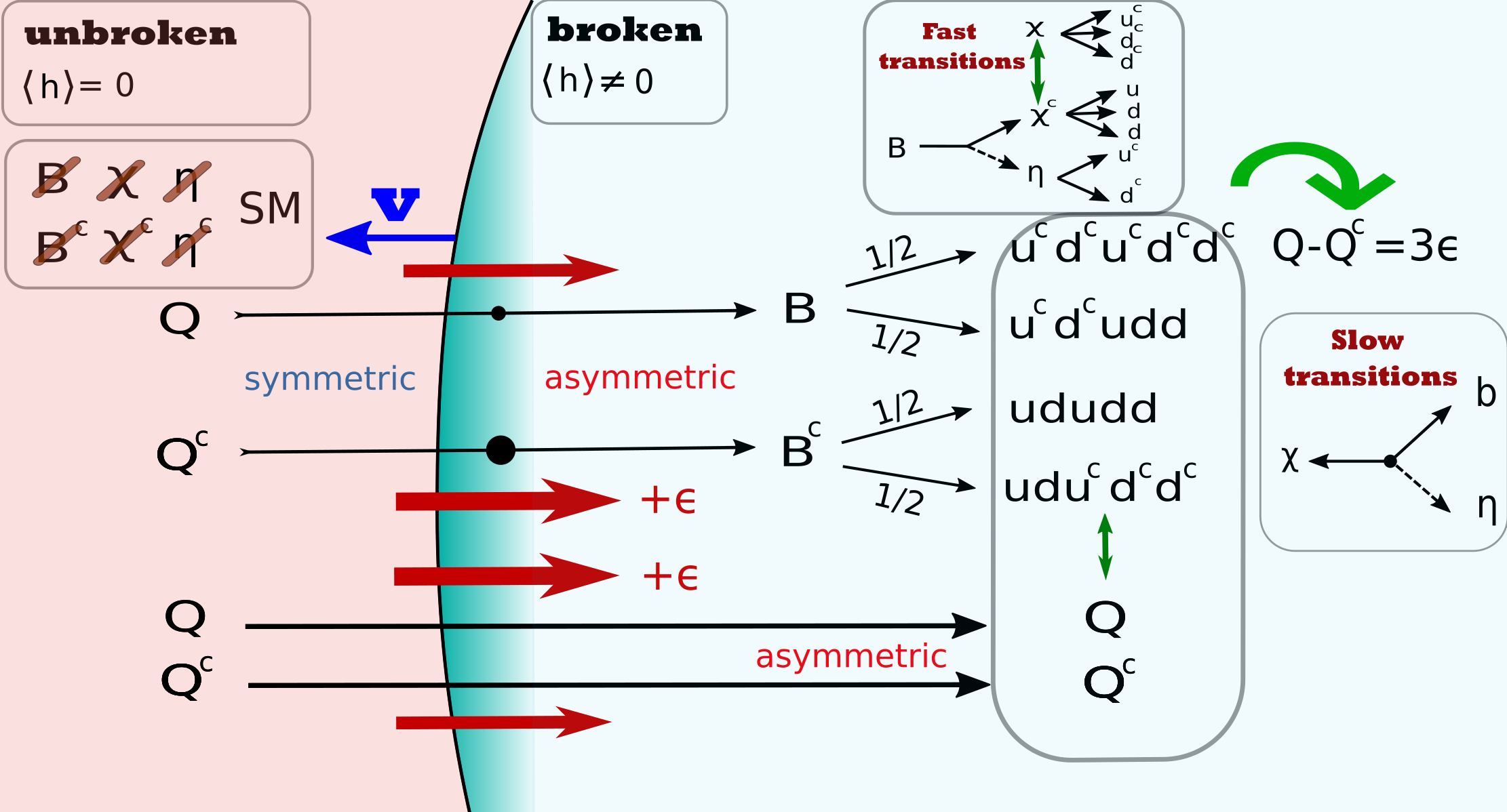
Figure 3: Mechanism at play in the low energy baryogenesis.

In the previous section we have presented a model generating the baryon asymmetry during the phase transition at the high scale. However we can wonder whether the mechanism proposed (in section 3.1) can be effective for generation of the baryon asymmetry during the EW phase transition. The necessary ingredient for the mechanism is a strong first order electroweak phase transition and various studies indicate that even a singlet scalar (see ref.[52, 53, 54, 55, 56, 57, 58]) or dimension six operator (see ref. [59, 60, 61, 62, 58]) extensions of SM can do the job. In this paper however we take an agnostic approach about the origin of such EW FOPT and just assume that it has happened with nucleation and reheating temperature as an input parameters and leave the detailed analysis of the explicit realizations for the future studies. Below we present a prototype model:

$${\cal L}= {\cal L}_{SM}+m_{\eta}^{2}|\eta|^{2}+\sum_{I=1,2}M_{I}\bar{B}_{I}B_{I}$$

$$+ \left(\sum_{I=1,2}Y_{I}(\bar{B}_{I}H)P_{L}Q+{y_{I}\eta^{*}\bar{B}_{I}P_{R}\chi}+\kappa\eta^{c}du+\frac{1}{2}m_{\chi}\bar{\chi^{c}}\chi+h.c.\right).$$ (53)

As before we do not write kinetic terms. The model contains a Majorana field $\chi$ and two vector-like $B$ quarks with the masses $M_{1,2}\sim m_{\chi}$. Here $\eta$ is a scalar field which is in the fundamental representation of QCD with electric charge $Q(\eta)=1/3$, $Q,u,d$ are the SM quark doublet and singlets respectively, we ignore the flavour indices for now, $H$ is the SM Higgs and we assume that the EW phase transition is of the first order with relativistic enough bubbles. Note that the interaction $LH\chi^{c}$ is consistent with all the gauge symmetries of the model, however we set it to zero in order to avoid proton decay. This can be attributed to some accidental discrete symmetry.

Let us assume that only the third generations couples to the heavy vector like $B$ quark, $Q=(t,b)$ in Eq.(3.2), then unlike the previous leptogenesis model, asymmetry will be generated when the relativistic SM $b$ quarks are hitting the wall.

Let us look at the baryon number assignments of the various fields in our lagrangian: $B(\eta)=2/3,B(\chi)=1$, so that the $m_{\chi}$ violates the baryon symmetry by two units. In this case, the story goes as follows: the sweeping of the relativistic wall, via the collision of the b-quarks with bubbles, produces $B_{I},B_{I}^{c}$. Thus inside the bubble

$$n_{B_{I}}-n_{B^{c}_{I}}=-\theta_{I}^{2}\epsilon_{I}n_{b}^{0}$$

$$n_{b}-n_{b^{c}}=\sum_{I}\theta_{I}^{2}\epsilon_{I}n_{b}^{0}$$ (54)

where $n_{b}$ is the number density of the bottom-type quark, $\theta_{I}\approx\frac{Y_{I}\langle{H}\rangle}{M_{I}}$ is the mixing angle and $\epsilon_{I}$ is defined like in Eq. (24) (in this case there is no $i$ index since we coupled it only to the third generation of quarks). CP asymmetry will be generated by the diagram represented on the Fig. 4 with $\chi,\eta$ fields running inside the loop.

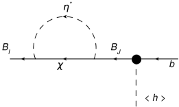
Figure 4: One loop diagram contributing to the $b\to B$ transition

The loop function generated by the diagram of Fig. 4 becomes

$${f_{B}^{IJ}(x)}=\int\frac{d^{4}p}{(2\pi)^{4}}\frac{P_{R}(\not{p}+m_{\chi})P_{L}(\not{p}_{out}+M_{J})P_{L}}{(p^{2}-m_{\chi}^{2}+i\epsilon)((p-p_{out})^{2}-m_{\phi}^{2}+i\epsilon)(p_{out}^{2}-M_{I}^{2}+i\epsilon)}$$ (55)

after taking the imaginary part, we obtain

$${\text{Im}[f^{IJ}_{B}(x)]}=\frac{1}{32\pi}\frac{M_{I}M_{J}}{M_{I}^{2}-M_{J}^{2}}\frac{\sqrt{(M_{I}^{2}-m_{\eta}^{2}+m_{\chi}^{2})^{2}-4m_{\chi}^{2}M_{I}^{2}}}{M_{I}^{4}}\left(M_{I}^{2}+m_{\chi}^{2}-m_{\eta}^{2}\right)$$ (56)

Compared to Eq. (27) we have an additional $1/2$ factor (at the massless limit of $\eta,\chi$) because $\eta,\chi$ are $SU(2)_{L}$ singlet now.

Similarly to our general discussion after the passage through the wall the following asymmetric abundances will be generated

$$\sum_{I}\left(n_{B_{I}}-n_{B_{I}^{c}}\right)=-(n_{b}-n_{b^{c}}).$$ (57)

Let us see what will happen after $B_{I}$ decays. There are two decay channels that lead back to b quarks and thus can erase the asymmetry, one which is direct back-decay to SM $B_{I}\to bh$ ($h$ is the CP even neutral component of the Higgs doublet) and the other through $\chi,\eta$, $B_{I}\to\chi\eta^{c}$ if kinematically allowed. The last channel will lead to the following decay chain

$$B_{I}\to\chi\eta^{c}\to\chi d^{c}u^{c}.$$ (58)

Let us look at the decays of the $\chi$ field. For concreteness we will assume the following ordering of the masses

$$M_{I}>m_{\chi}>M_{\eta}.$$ (59)

Then the Majorana fermion $\chi$ is not stable and decays

$$\chi\to b\eta,$$ (60)

where $\chi^{c}b\eta$ interaction is generated after EWSB due to the mixing between vectorlike quarks and SM fields once the Higgs boson develops the VEV. The $\eta$ field later decays to two quarks. However the Majorana nature of the field $\chi$ makes the decay to the CP conjugate final state open as well so that

$$\chi\to b\eta\to bdu$$

$$\chi\to b^{c}\eta^{c}\to b^{c}d^{c}u^{c},$$ (61)

decays are allowed and both final states have the same probabilities. As a result there will be two decay chains of $B$ one leading to the generation of the baryon asymmetry and another to the wash-out

$$(i)~{}~{}\text{wash-out}:~{}~{}B_{I}\to\chi d^{c}u^{c}\to(bdud^{c}u^{c})\qquad~{}~{}B_{I}^{c}\to\chi^{c}du\to(b^{c}d^{c}u^{c}du)$$

$$(ii)~{}~{}\text{asymm. generation}:~{}~{}B_{I}\to\chi^{c}d^{c}u^{c}\to(b^{c}d^{c}u^{c}d^{c}u^{c})\qquad~{}~{}B_{I}^{c}\to\chi du\to(bdudu)$$

(62)

As a result the asymmetry between SM quarks and antiquarks will be given

$$(n_{q}-n_{q^{c}}) =\sum_{I}(n_{B_{I}}-n_{B_{I}^{c}})\left[\left(-\frac{5}{2}+\frac{1}{2}\right)Br(B_{I}\to\chi\eta^{c})+Br(B_{I}\to bh)\right]+(n_{b}-n_{b^{c}})$$

, $$=-3\sum_{I}(n_{B_{I}}-n_{B_{I}^{c}})Br(B_{I}\to\chi\eta^{c}),$$ (63)

where we have used $Br(B_{I}\to\chi\eta^{c})+Br(B_{I}\to bh)=1$ and Eq.57 to derive the last relation. At last we have to take into account CP violating decays of the $B$ particles similarly to the discussion in Eq.(37)

$$\epsilon^{I}_{decay}=\frac{\Gamma(B^{I}\to\chi\eta^{c})-\Gamma(B^{I,c}\to\chi^{c}\eta)}{\Gamma(B^{I,c}\to\chi\eta^{c})+\Gamma(B^{I,c}\to\chi^{c}\eta)}=-\frac{4{\rm Im}(Y_{I}Y^{*}_{J}y_{I}^{*}y_{J}){\rm Im}[f_{B}^{IJ}]|_{m_{\eta,\chi}\to 0}}{|y_{I}|^{2}}$$ (64)

where the loop function is exactly equal to the one in Eq. (56) with zero masses of the particles inside the loop and an extra factor of 2, since inside the loop will now circulate the EW doublet. Thus for the total baryon asymmetry we obtain

$$\frac{\Delta n_{Baryon}}{s}\approx \frac{135\zeta(3)}{8\pi^{4}}\sum_{I,J}\theta_{I}^{2}\frac{|y_{I}|^{2}}{|y_{I}|^{2}+|Y_{I}|^{2}}\times\frac{g_{b}}{g_{\star}}\bigg{(}\frac{T_{\rm nuc}}{T_{reh}}\bigg{)}^{3}$$ (65)

$$\times{\rm Im}(Y_{I}Y^{*}_{J}y_{I}^{*}y_{J})\left(-\frac{2{\rm Im}[f_{B}^{IJ}]}{|Y_{I}|^{2}}+\frac{4{\rm Im}[f_{B}^{IJ}]|_{m_{\chi,\eta}\to 0}}{|y_{I}|^{2}}\right).$$

With $\frac{135\zeta(3)}{8\pi^{4}}\times\frac{|y_{I}|^{2}}{|y_{I}|^{2}+|Y_{I}|^{2}}\times\frac{g_{b}}{g_{\star}}\frac{{\rm Im}[Y_{2}Y_{1}^{*}y_{2}^{*}y_{1}]}{16\pi|Y_{I}|^{2}}\sim 10^{-(3-4)}$ and $g_{b}=6$ being the degrees of freedom of $b$ quark and assuming $y_{I}=O(1)$ and $|y_{I}|\gg|Y_{I}|\sim|Y_{J}|$, recovering the observed baryon abundance $\frac{\Delta n_{Baryon}}{s}\sim 8.8\times 10^{-11}$ requires, in order of magnitude,

$$\Rightarrow\boxed{\theta_{I}^{2}\bigg{(}\frac{T_{\rm nuc}}{T_{reh}}\bigg{)}^{3}\sim 10^{-(6-7)}}.$$ (66)

The decay chains described above are very fast compared to the Hubble scale so that we can treat them as instantaneous. Indeed the

$$\Gamma(\chi\to\eta b)\approx\left|\sum_{I}y_{I}\theta_{I}\right|^{2}\frac{m_{\chi}(1-m_{\eta}^{2}/m_{\chi}^{2})}{8\pi g_{\chi}}\Rightarrow$$ (67)

$$\frac{\Gamma(\chi\to\eta b)}{H(v_{EW})}\simeq 10^{-3}\frac{M_{p}}{m_{\chi}}\gg 1,$$ (68)

since in the range of interest $\theta\lesssim 10^{-2}\Rightarrow m_{\chi}<10^{2}$ TeV.

Thus, after this first phase of very fast decays, that produces the baryon asymmetry in the quark sector, slow transition mediated by the heavy states can still wash out the asymmetry. In this part, we check for which region of the parameter space it is not the case. The various wash-out transitions include

• $b\eta\to\chi$
  The decoupling of this transition provides the following condition, reminiscent of Eq.(49). In particular writing the Boltzmann in equation for the B-asymmetry we will get:

  $$szH(z)\frac{d(Y_{b}-Y_{b^{c}})}{dz}\simeq-\gamma_{\chi\to\eta b}\left(\frac{Y_{b}Y_{\eta}-Y_{b^{c}}Y_{\eta^{c}}}{Y_{b}^{eq}Y_{\eta}^{eq}}\right)$$ (69)

  assuming that the asymmetries in $B$ and $\eta$ are related as follows

  $$Y_{b,b^{c}}=(1\pm\epsilon_{q})Y_{eq}^{b},~{}~{}~{}Y_{\eta,\eta^{c}}\simeq Y_{eq}^{\eta}$$ (70)

  then, we arrive at the following equation

  $$szH(z)\frac{d(\epsilon_{q}Y_{eq})}{dz}\simeq-\gamma_{\chi\to\eta b}\epsilon_{q},~{}~{}~{}\gamma_{\chi\to\eta b}=\frac{g_{\chi}T^{3}}{2\pi^{2}}z^{2}K_{1}(z)\Gamma(\chi\to\eta b)$$

  $$\frac{d\epsilon_{q}}{dz}=-\frac{0.42e^{-z}z^{5/2}}{g_{*}^{1/2}g_{q}}\left(\frac{M_{p}}{m_{\chi}}\right)\left(\frac{g_{\chi}\Gamma(\chi\to\eta b)}{m_{\chi}}\right)\epsilon_{q}$$

  $$\Gamma(\chi\to\eta b)\approx\left|\sum_{I}y_{I}\theta_{I}\right|^{2}\frac{m_{\chi}(1-m_{\eta}^{2}/m_{\chi}^{2})}{8\pi g_{\chi}}$$ (71)

  Then the process is decoupled for the temperatures of EW scale if $m_{\chi}/T_{reh}\gtrsim 30$, which pushes us to the limits of the maximal asymmetry which we can achieve in the mechanism. Indeed assuming $T_{reh}\sim 100$ GeV, we are required to have $m_{\chi}\gtrsim 3$ TeV and $m_{B}\gtrsim 3$ TeV. Note that on top of the process above there will be reactions $\eta b\to\eta^{c}b^{c}$ which will also lead to the wash out of the asymmetry. This process is suppressed by the Boltzmann factor for $\eta$ field abundance so that the condition to not erase the asymmetry becomes

  $$\frac{m_{B,\chi,\eta}}{T_{reh}}\gtrsim 30.$$ (72)

• $ddu\leftrightarrow d^{c}d^{c}u^{c}$
  After integrating out all the new heavy fields the following baryon violating number operator is obtained.

  $$\frac{ddu\overline{d^{c}d^{c}u^{c}}}{M_{\eta}^{4}}\times\frac{1}{m_{\chi}}\times\theta^{2}\qquad\Rightarrow\qquad{\frac{1}{4\pi^{5}}\bigg{(}\frac{1}{16\pi^{2}}\bigg{)}^{2}}\frac{T_{reh}^{11}}{M_{\eta}^{8}m_{\chi}^{2}}\theta^{4}\lesssim\frac{T_{reh}^{2}}{M_{p}}.$$ (73)

  However, it can easily be seen that the rate of the baryon number violating processes mediated by it are much slower than the Hubble expansion as well.

3.2.1 Experimental signatures

This low-energy model has the interesting consequence that it induces potential low-energy signatures. In this section, we enumerate those possible signatures without assuming that $Q,u,\text{and }d$ are the third generation quarks.

Neutron oscillations

The baryon number violating processes in the model will violate the baryon number only by $2$ units, so proton decay is not allowed but $n-\bar{n}$ oscillations can be present[63]. Integrating out the heavy states, we obtain the following operator

$$\frac{1}{\Lambda^{5}_{n\bar{n}}}\overline{u^{c}d^{c}d^{c}}udd\equiv\frac{(\sum{\kappa\theta_{I}y_{I}})^{2}}{M_{\eta}^{4}m_{\chi}}\overline{u^{c}d^{c}d^{c}}udd$$ (74)

thus inducing a neutron mixing mass of the form

$$\delta m_{\bar{n}-n}\sim\frac{\Lambda_{QCD}^{6}}{M_{\eta}^{4}m_{\chi}}(\sum{\kappa\theta_{I}y_{I}})^{2}.$$ (75)

Current bounds on this mixing mass are of order $\delta m_{\bar{n}-n}\lesssim 10^{-33}$ GeV [64, 65, 66, 67, 68]. This is extremely significant if the SM quarks in the Lagrangian are in first or second generation. If we take order 1 couplings and $\theta^{2}\sim 10^{-5}$, it places a bound on the typical mass scale of

$$\Lambda_{n\bar{n}}\gtrsim 10^{6}{\rm GeV}~{}~{}~{}(M_{\eta},m_{\chi})\gtrsim 10^{5}\text{GeV}$$ (76)

This bound becomes weaker if the new particles couple only to the third generation. Then we have an additional suppression factor $(V_{td}^{4}V_{bu}^{2})^{1/5}\sim 10^{-2}$. As a consequence, depending on the flavor of $Q,u,d$ our scenario can be tested in the future experiment [69, 70, 71, 72].

Flavor violation

The model predicts new particles in the $1-10^{3}$ TeV range coupled to the SM light quarks- $\eta$ field. So the question about low energy bounds naturally rises. However the FCNC are absent at tree level for the $\eta$-diquark field [73]. The loop level effects can lead to strong constraints if $\eta du$ coupling contains the light generation quarks [73], but if $du$ are only the third generation fields $t_{R},b_{R}$ the bounds are practically absent.

Bounds from EDMs

If there is CP violation in the mixing between bottom quark and heavy bottom partners then we expect an operator of the form

$$-i\frac{g_{3}\tilde{d}_{q}}{2}\bar{Q}\sigma^{\mu\nu}T^{A}\gamma_{5}QG^{A}_{\mu\nu}$$ (77)

which is the chromo-electric dipole moment (see [74] for a review) with coefficient scaling like

$$\tilde{d}_{q}\sim\text{Im}[y_{I}^{2}]\frac{\theta_{I}^{2}m_{b}}{16\pi^{2}}\frac{1}{\Lambda_{EDM}^{2}}$$ (78)

where $\Lambda_{EDM}\sim M_{\eta}\sim m_{\chi}\sim(1-100)$ TeV is the scale of the new physics that we are considering. Up-to-date bounds [75, 76] are $\tilde{d}_{b}<1.2\times 10^{-20}cm\sim 10^{-6}GeV^{-1}$ , which include the nucleon EDM bound via the RG effect. Taking typical values of the mixing angle $\theta^{2}\sim 10^{-4}$, it can be seen that those bounds are not stringent.

Electron EDM is known to be one of the important test of the EW baryogenesis theories. In our model the leading contribution appears at three loop level due to the Barr-Zee type [77] of diagram with $b-B$ mixing. The estimate of the dipole operator goes like

$$\frac{d_{e}}{e}\sim\frac{m_{e}(yYe)^{2}}{(4\pi)^{6}}\bigg{(}\frac{1}{\Lambda_{EDM}^{2}}\bigg{)}\sim 3\times 10^{-33}\times\left(\frac{10{\rm TeV}}{\Lambda_{EDM}}\right)^{2}{\rm cm}$$ (79)

which is four orders of magnitude below the current experimental bound [78] $|d_{e}|<1.1\times 10^{-29}{\rm cm}\cdot e$ .

Gravitational waves

One very robust prediction of such a scenario is the large amount of GW emitted at the transition, with peak frequency fixed by the scale of the transition $f_{\text{peak}}\sim 10^{-3}\frac{T_{\text{reh}}}{\text{GeV}}$ mHz (see [79] for review). Such SGWB signal could be detected in future GW detectors such as LISA[80, 81], eLISA[82], LIGO[83, 84], BBO[85, 86], DECIGO[87, 88, 89], ET[90, 91, 92], AION[93], AEDGE[94]. This array of observers will be able to probe GW with frequencies in the window of mHz to kHz, which is the optimal scale for this mechanism to take place.

Direct production in colliders

An almost coupling- and flavor-independent bound is the LHC one. The heavy quark can be produced via the strong or electro-magnetic interaction. From the recent squark or gluino bounds in the LHC e.g.[95, 96], we expect a mass bound of $\sim 2$ TeV on the lightest colored particle.

3.2.2 Parameter region

By combining all the previous bounds and by numerically solving the washout condition Eq.(71) we show the parameter region of this scenario in Fig.5. Here the horizontal axis is the $T_{\rm nuc}$ which, in order to produce a relativistic bubble wall, is favored to be smaller than $T_{\rm reh}$, which we took equal to $100$ GeV. The vertical axis denotes $M_{\eta}(<M_{I}),$ which is the lightest diquark in this scenario. All the data points give the correct baryon asymmetry $\Delta n_{B}/s=8.8\times 10^{-11},$ with all the couplings smaller than $\sqrt{2\pi}.$ The green points satisfy the bound on $n-\bar{n}$ oscillation in Eq.(76). The red and blue points do not satisfy it, which implies a special flavor structure for example that only $b$ is coupled to the BSM particles. For both red and green points, both $M_{1}$ and $M_{2}$ satisfy the relativistic wall condition (88) in the appendix, which is denoted by the black solid line. For the blue points, the lighter of $M_{1}$ and $M_{2}$ satisfies the condition. The horizontal dotted at 2 TeV is the typical bound on new colored particles. Therefore our mechanism predicts light quark, which may be searched for in the LHC and future colliders. Moreover, since our data points include parameter space both consistent and inconsistent with the neutron-anti-neutron oscillation bound, some points with BSM particles that also couple to the first two generation quarks can be tested in the future. Note again that $T_{\rm nuc}\sim O(0.1)T_{\rm reh}$ may be the consistent range for our scenario to work.

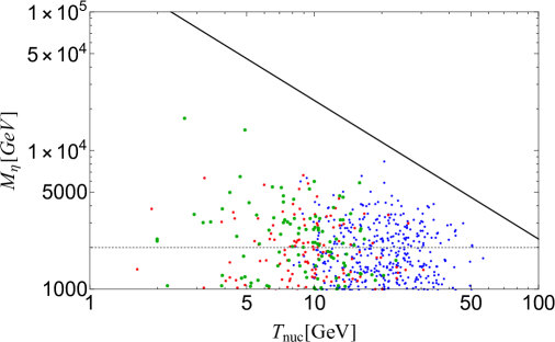
Figure 5: $M_{\eta}$ (which is the lightest colored particle mass) vs $T_{\rm nuc}$ in the low energy baryogenesis. The green points satisfy (76), while the red and blue points do not satisfy it and thus require a special flavor-structure. Both (the lighter of) $M_{1}$ and $M_{2}$ are taken to satisfy the conditions from maximal wall velocity (88), which is shown by the black solid line, in the appendix for green and red (blue) points. Here we fix $\langle{H}\rangle=T_{\rm reh}=100\,$GeV to consider the electroweak phase transition and fix $\Delta n_{B}/s=8.8\times 10^{-11}$. Other parameters are randomly chosen within the perturbative unitarity range. Below the 2TeV (dotted line) may be disfavored by the null detection of new colored particle in the LHC.

3.2.3 Baryogenesis from non-EW FOPT

At last we note that, with a simple modification of the model in Eq.(3.2), the mechanism can be operative for an arbitrary phase transition. Indeed let us assume that $\phi$ is the field experiencing the FOPT then the following lagrangian :

$${\cal L}_{\phi}={\cal L}_{SM}+\sum_{I=1,2}\tilde{Y}_{I}(\bar{B}_{I}\phi)b_{R}+M_{I}\bar{B}_{I}B_{I}+\lambda_{I}B_{I}\chi^{c}\eta+\kappa\eta^{c}du+\frac{m_{\chi}}{2}\bar{\chi}^{c}\chi$$ (80)

can induce the required baryon asymmetry. The phenomenology remains similar to the model of Eq.(3.2) however the experimental constraints from $n-\bar{n}$ oscillations and other low energy searches become even weaker. At the limit, the only robust experimental signature of such a scenario is the GW background emitted if the VEV is not extremely larger than the EW scale.

4 Summary

In this paper we have presented a novel mechanism for the generation of the baryon asymmetry during the early universe evolution. We have first shown that the mechanism of production of the heavy particles from the relativistic bubble expansion during the FOPT can lead to CP violating effects. This mechanism of particle production is out of equilibrium, so that if baryon number violating interactions are present a baryon asymmetry can be generated. We have constructed two viable baryogenesis models implementing this idea. The first scenario is the phase-transition-induced leptogenesis, where the bubble wall should be composed by some new Higgs field charged under the lepton number, and after the phase transition we are still in the symmetric phase of the EW interactions but in the broken phase of the lepton number. Later EW spharelons transfer the lepton asymmetry to the baryon sector. In this scenario, a net $B-L$ asymmetry is generated since the Majorana term of the right-handed neutrino after the PT violates the $B-L$ symmetry. Neutrino mass observations make the mechanism viable if the scale of the phase transition is between $[10^{9},10^{12}]$ GeV, which makes it borderline detectable for the future gravitational wave experiments such as ET[90, 91, 92]. The second scenario can happen during EW phase transition. In this case, new fields charged under QCD with $\lesssim 100$ TeV scale masses are needed to have enough baryon number production. In both cases the baryon/lepton number violating interactions are coming from the Majorana masses of new heavy particles. This leads to the Majorana neutrino masses in the first class of models and $n-\bar{n}$ oscillations in the second class of models. Another feature of this mechanism is that baryogenesis happens for the ultra-fast bubble expansions thus generically strong stochastic gravitational wave signatures are expected. Moreover, in the case of the second scenario, the frequency range is well within the reach of the current and future experiments.

Note added : when this paper was close to completion we have become aware of another project discussing the baryon asymmetry generation due to the heavy particles production in phase transition [97].

Appendix A Dynamics of the transition

In our discussion of the phase transition we have been completely agnostic regarding the origin of the potential and treated the Lorentz factor $\gamma_{w}$ as a free input parameter. This is obviously not the case and the nature of the phase transitions as well as the dynamics of the bubble expansion depend on the details of the potential and the particle content. However even without going into explicit models we can make few semi-quantitative claims on whether the values of $\gamma_{w}$ needed for the heavy particles production can be achieved or not. In this respect it is important to recall the forces acting on the wall, which determine the velocity of the expansion of the bubbles. First of all there is a driving force which is given by the potential differences between true and false vacua

$$\hbox{Driving force}=V_{false}-V_{true}\equiv\Delta V,$$ (81)

and then there are friction forces due to the plasma particles colliding with the bubble walls. Generically the calculation of these effects is quite involved but for the relativistic expansions $\gamma_{w}\gg 1$ calculations become much simpler. At tree level (leading order LO), the pressure from the plasma on the bubble wall [98, 99] has the form:

$$\Delta\mathcal{P}_{\text{LO}}\to\sum_{i}g_{i}c_{i}\frac{\Delta m_{i}^{2}}{24}T_{\text{nuc}}^{2},$$ (82)

where $T_{\rm nuc}$ is the nucleation temperature (roughly temperature when the PT occurs) and $\Delta m^{2}_{i}$ is the change of the masses of the particle $i$ during the PT and $c_{i}=1(1/2)$ for bosons(fermions). In the presence of the mixing between light particles and heavy particles, which is exactly our scenario of production of out-of-equilibrium heavy states, there is a second LO friction contribution from the mixing [1]. For the models under consideration, this friction takes the form

$$\Delta\mathcal{P}^{mixing}_{\text{LO}}\to\frac{T^{2}Y^{2}}{48}\langle{\phi}\rangle^{2}\Theta(\gamma_{w}T_{\rm nuc}-M^{2}L_{w})$$ (83)

and in this section we consider that $\langle{\phi}\rangle$ is the scale of the symmetry breaking. At last in the presence of the gauge bosons which gain mass during the phase transition the pressure receives Next-To-Leading order (NLO) correction[100]

$$\Delta\mathcal{P}_{\text{NLO}} \simeq \sum_{i}g_{i}g_{gauge}^{3}\gamma_{w}T_{\text{nuc}}^{3}\frac{\langle{\phi}\rangle}{16\pi^{2}},$$ (84)

where $g_{gauge}$ is the gauge coupling. Unlike the LO pressure contributions this effect is growing with $\gamma_{w}$ thus eventually stopping the accelerated motion of the bubbles. In order to estimate the maximal value of the $\gamma_{w}$ achievable during the FOPT let us consider the bubble expansion in two cases; i.e. with and without the $\gamma_{w}$ dependent friction (that is to say, with and without gauge bosons).

1. Friction is independent on $\gamma_{w}$ (no phase dependent gauge fields). In this case, if $\Delta V>\mathcal{P}_{LO}$, the bubbles will keep accelerating till the collision and the $\gamma_{w}$ at collision can be estimated as [103, 104],

   $$\gamma_{w,\rm MAX}\simeq\frac{2R_{*}}{3R_{0}}\left(1-\frac{\mathcal{P}_{\rm LO}}{\Delta V}\right),\quad R_{0}\sim 1/T_{\text{nuc}},\quad R_{*}\approx\frac{(8\pi)^{1/3}v_{w}}{\beta(T_{\rm nuc})},~{}~{}~{}\beta(T)=HT\frac{d}{dT}\left(\frac{S_{3}}{T}\right)$$

   $$\Rightarrow\gamma_{w,\rm MAX}\sim\frac{M_{\text{p}}T_{{\rm nuc}}}{\langle{\phi}\rangle^{2}}$$ (85)

   where $R_{\star}$ is an estimate for the bubble size at collision and $R_{0}$ is the bubble size at nucleation and $\beta$ the inverse duration parameter of the transition.

2. Friction depends on $\gamma_{w}$: (gauge symmetry is broken during the PT). In this case equating the friction and the driving force gives the maximal velocity of the bubble;

   $$\Delta V=\Delta\mathcal{P}_{\text{NLO}}(\gamma_{w}\equiv\gamma_{w,\text{MAX}})\qquad\Rightarrow\gamma_{w,\text{MAX}}\approx\frac{16\pi^{2}}{g_{gauge}^{3}}\bigg{(}\frac{\langle{\phi}\rangle}{T_{{\rm nuc}}}\bigg{)}^{3}.$$ (86)

Combining the results for the two regimes of the bubble expansion we get

$$\gamma_{w}^{MAX}=\hbox{Min}\left[\frac{16\pi^{2}}{g_{gauge}^{3}}\bigg{(}\frac{\langle{\phi}\rangle}{T_{{\rm nuc}}}\bigg{)}^{3},\frac{M_{\text{p}}T_{{\rm nuc}}}{\langle{\phi}\rangle^{2}}\right]~{}~{}\hbox{if}~{}~{}\Delta V>\Delta{\cal P}_{\rm LO}.$$ (87)

This results in the maximal mass of the heavy states which can be produced during the PT which is given by

$$M^{MAX}\sim\text{Min}\left[\frac{4\pi}{g_{gauge}^{3/2}}\frac{\langle{\phi}\rangle^{2}}{T_{\rm nuc}},\frac{M_{p}^{1/2}T_{\rm nuc}}{\langle{\phi}\rangle^{1/2}}\right]$$ (88)

If we assume $T_{\rm nuc}\sim(0.1-0.01)\langle{\phi}\rangle$, then for EW phase transition the maximal mass of the state we can produce becomes

$$M^{MAX}_{EW}\sim(10^{2}-10^{3})v_{EW}\sim(10-100){\rm TeV}$$ (89)

So that the model in the section 3.2 immediately satisfies this criteria. The same is true as well for the model in section 3.1 since in this case

$$M^{MAX}\sim(0.3-0.1)\sqrt{M_{p}\langle{\phi}\rangle}$$ (90)

and, for an efficient production of heavy states we needed $10^{-(2-3)}\lesssim\theta\sim\frac{\langle{\phi}\rangle}{M}$.

Appendix B Variations on the models

In this appendix, we will list the modifications of the models presented in the main text in Section 3, which can realize a successful baryogenesis scenario with significantly different phenomenology.

B.1 Alternative Phase-transition induced leptogenesis

The simplest modification we can take of the Eq.(3.1) is the consider the opposite chiralities;

$$\mathcal{L}_{\text{int}} = \underbrace{\sum_{iI}\bigg{(}Y_{iI}(\phi\bar{\chi}_{i})P_{R}N_{I}+Y_{iI}^{\star}\bar{N}_{I}P_{L}(\phi^{\dagger}\chi_{i})\bigg{)}-V(\phi)+\sum_{i}\lambda_{\chi}\phi\bar{\chi}^{c}_{i}\chi_{i}+\sum_{I}M_{I}\bar{N}_{I}N_{I}}_{\text{Toy model of Dark Sector}}$$

$$+ \underbrace{\sum_{\alpha I}y_{\alpha I}(h\bar{l}_{\alpha,SM})P_{R}N_{I}+h.c.}_{\text{Connection to SM}}$$

In this case the generation of CP asymmetry proceeds in the similar way to the discussion above but neutrino masses are generated at one loop level. As a result parameter space with lower masses $m_{\chi}$ by around two orders of magnitude becomes accessible. We leave the thorough study of this case to further studies.

B.2 Alternative baryogenesis models

Let us here enumerate the possible change that we can make in the Lagrangian of Eq.(3.2)

• We can couple $\eta$ instead of the right-handed to the left-handed ones via $\eta^{c}QQ$.

• We can also couple the opposite chirality to the the diquark with the coupling $y\eta\chi P_{R}B$. In the case of the coupling $y\eta\chi P_{R}B$, on the top of the previous estimates, there will be an additional $m_{b}/M_{B}$ suppression in the $\chi$ decay and a similar $m_{b}^{2}/M_{B}^{2}$ is the $n-\bar{n}$ oscillations.

• We may also replace $B_{i}$ by an up-type-like quark, and assume that it mainly couples to the top quarks, this effect is suppressed by a further Boltzmann factor. Then the Lagrangian is given as

  $$\sum_{i=1,2}Y_{i}(\bar{U}_{i}H^{*})Q+M_{Bi}\bar{U}_{i}U_{i}+\lambda_{i}U_{i}\chi^{c}\eta+\kappa\eta^{c}dd+\frac{m_{\chi}}{2}\bar{\chi}^{c}\chi+m_{\eta}|\eta|^{2}.$$ (92)

  Here $dd$ denotes $(d_{2}d_{3}$ or $d_{1}d_{2})$. The FCNC constraint is stringent but there is a viable parameter region.

References

- [1] A. Azatov and M. Vanvlasselaer JCAP 01 (2021) 058, [arXiv:2010.02590].
- [2] Planck Collaboration, P. A. R. Ade et al. Astron. Astrophys. 594 (2016) A13, [arXiv:1502.01589].
- [3] A. D. Sakharov Pisma Zh. Eksp. Teor. Fiz. 5 (1967) 32–35. [Usp. Fiz. Nauk161,no.5,61(1991)].
- [4] A. Riotto, Theories of baryogenesis, in ICTP Summer School in High-Energy Physics and Cosmology, 7, 1998. hep-ph/9807454.
- [5] D. Bodeker and W. Buchmuller arXiv:2009.07294.
- [6] T. Bhattacharya et al. Phys. Rev. Lett. 113 (2014), no. 8 082001, [arXiv:1402.5175].
- [7] K. Kajantie, M. Laine, K. Rummukainen, and M. E. Shaposhnikov Phys. Rev. Lett. 77 (1996) 2887–2890, [hep-ph/9605288].
- [8] V. Kuzmin, V. Rubakov, and M. Shaposhnikov Phys. Lett. B 155 (1985) 36.
- [9] M. Shaposhnikov JETP Lett. 44 (1986) 465–468.
- [10] A. E. Nelson, D. B. Kaplan, and A. G. Cohen Nucl. Phys. B 373 (1992) 453–478.
- [11] M. Carena, M. Quiros, and C. E. M. Wagner Phys. Lett. B 380 (1996) 81–91, [hep-ph/9603420].
- [12] J. M. Cline Phil. Trans. Roy. Soc. Lond. A 376 (2018), no. 2114 20170116, [arXiv:1704.08911].
- [13] S. Bruggisser, B. Von Harling, O. Matsedonskyi, and G. Servant JHEP 12 (2018) 099, [arXiv:1804.07314].
- [14] S. Bruggisser, B. Von Harling, O. Matsedonskyi, and G. Servant Phys. Rev. Lett. 121 (2018), no. 13 131801, [arXiv:1803.08546].
- [15] D. E. Morrissey and M. J. Ramsey-Musolf New J. Phys. 14 (2012) 125003, [arXiv:1206.2942].
- [16] A. J. Long, A. Tesi, and L.-T. Wang JHEP 10 (2017) 095, [arXiv:1703.04902].
- [17] C. Caprini and J. M. No JCAP 01 (2012) 031, [arXiv:1111.1726].
- [18] J. M. Cline and K. Kainulainen Phys. Rev. D 101 (2020), no. 6 063525, [arXiv:2001.00568].
- [19] G. C. Dorsch, S. J. Huber, and T. Konstandin arXiv:2106.06547.
- [20] A. Katz and A. Riotto JCAP 11 (2016) 011, [arXiv:1608.00583].
- [21] A. Azatov, M. Vanvlasselaer, and W. Yin JHEP 03 (2021) 288, [arXiv:2101.05721].
- [22] G. Lazarides and Q. Shafi Phys. Lett. B 258 (1991) 305–309.
- [23] T. Asaka, K. Hamaguchi, M. Kawasaki, and T. Yanagida Phys. Lett. B 464 (1999) 12–18, [hep-ph/9906366].
- [24] K. Hamaguchi, H. Murayama, and T. Yanagida Phys. Rev. D 65 (2002) 043512, [hep-ph/0109030].
- [25] R. Barbier et al. Phys. Rept. 420 (2005) 1–202, [hep-ph/0406039].
- [26] S. Dimopoulos and L. J. Hall Phys. Lett. B 196 (1987) 135–141.
- [27] K. S. Babu, R. N. Mohapatra, and S. Nasri Phys. Rev. Lett. 97 (2006) 131301, [hep-ph/0606144].
- [28] D. McKeen and A. E. Nelson Phys. Rev. D 94 (2016), no. 7 076002, [arXiv:1512.05359].
- [29] K. Aitken, D. McKeen, T. Neder, and A. E. Nelson Phys. Rev. D 96 (2017), no. 7 075009, [arXiv:1708.01259].
- [30] G. Elor, M. Escudero, and A. Nelson Phys. Rev. D 99 (2019), no. 3 035031, [arXiv:1810.00880].
- [31] C. Grojean, B. Shakya, J. D. Wells, and Z. Zhang Phys. Rev. Lett. 121 (2018), no. 17 171801, [arXiv:1806.00011].
- [32] Y. Hamada, R. Kitano, and W. Yin JHEP 10 (2018) 178, [arXiv:1807.06582].
- [33] A. Pierce and B. Shakya JHEP 06 (2019) 096, [arXiv:1901.05493].
- [34] T. Asaka, H. Ishida, and W. Yin JHEP 07 (2020) 174, [arXiv:1912.08797].
- [35] M. Fukugita and T. Yanagida Phys. Lett. B 174 (1986) 45–47.
- [36] J. A. Harvey and M. S. Turner Phys. Rev. D 42 (1990) 3344–3349.
- [37] P. Minkowski Phys. Lett. B 67 (1977) 421–428.
- [38] T. Yanagida Conf. Proc. C 7902131 (1979) 95–99.
- [39] M. Gell-Mann, P. Ramond, and R. Slansky Conf. Proc. C 790927 (1979) 315–321, [arXiv:1306.4669].
- [40] S. L. Glashow NATO Sci. Ser. B 61 (1980) 687.
- [41] R. N. Mohapatra and G. Senjanovic Phys. Rev. Lett. 44 (1980) 912.
- [42] S. Davidson, E. Nardi, and Y. Nir Phys. Rept. 466 (2008) 105–177, [arXiv:0802.2962].
- [43] P. Creminelli, A. Nicolis, and R. Rattazzi JHEP 03 (2002) 051, [hep-th/0107141].
- [44] G. Nardini, M. Quiros, and A. Wulzer JHEP 09 (2007) 077, [arXiv:0706.3388].
- [45] T. Konstandin and G. Servant JCAP 1112 (2011) 009, [arXiv:1104.4791].
- [46] A. Azatov and M. Vanvlasselaer JHEP 09 (2020) 085, [arXiv:2003.10265].
- [47] M. Carena, A. Megevand, M. Quiros, and C. E. Wagner Nucl. Phys. B 716 (2005) 319–351, [hep-ph/0410352].
- [48] A. Angelescu and P. Huang Phys. Rev. D 99 (2019), no. 5 055023, [arXiv:1812.08293].
- [49] T. Charnock, A. Avgoustidis, E. J. Copeland, and A. Moss Phys. Rev. D 93 (2016), no. 12 123503, [arXiv:1603.01275].
- [50] T. Hiramatsu, M. Kawasaki, and K. Saikawa JCAP 02 (2014) 031, [arXiv:1309.5001].
- [51] M. Gorghetto, E. Hardy, and H. Nicolaescu JCAP 06 (2021) 034, [arXiv:2101.11007].
- [52] G. W. Anderson and L. J. Hall Phys. Rev. D 45 (Apr, 1992) 2685–2698.
- [53] J. Choi and R. R. Volkas Phys. Lett. B 317 (1993) 385–391, [hep-ph/9308234].
- [54] J. R. Espinosa and M. Quiros Phys. Lett. B 305 (1993) 98–105, [hep-ph/9301285].
- [55] S. Profumo, M. J. Ramsey-Musolf, and G. Shaughnessy JHEP 08 (2007) 010, [arXiv:0705.2425].
- [56] J. R. Espinosa, T. Konstandin, and F. Riva Nucl. Phys. B 854 (2012) 592–630, [arXiv:1107.5441].
- [57] C.-Y. Chen, J. Kozaczuk, and I. M. Lewis JHEP 08 (2017) 096, [arXiv:1704.05844].
- [58] J. Ellis, M. Lewicki, and J. M. No JCAP 04 (2019) 003, [arXiv:1809.08242].
- [59] M. Chala, C. Krause, and G. Nardini JHEP 07 (2018) 062, [arXiv:1802.02168].
- [60] F. P. Huang, P.-H. Gu, P.-F. Yin, Z.-H. Yu, and X. Zhang Phys. Rev. D 93 (2016), no. 10 103515, [arXiv:1511.03969].
- [61] D. Bodeker, L. Fromme, S. J. Huber, and M. Seniuch JHEP 02 (2005) 026, [hep-ph/0412366].
- [62] C. Delaunay, C. Grojean, and J. D. Wells JHEP 04 (2008) 029, [arXiv:0711.2511].
- [63] K. Fridell, J. Harz, and C. Hati arXiv:2105.06487.
- [64] M. Baldo-Ceolin et al. Z. Phys. C 63 (1994) 409–416.
- [65] Super-Kamiokande Collaboration, K. Abe et al. Phys. Rev. D 91 (2015) 072006, [arXiv:1109.4227].
- [66] S. Rao and R. Shrock Phys. Lett. B 116 (1982) 238–242.
- [67] M. I. Buchoff, C. Schroeder, and J. Wasem PoS LATTICE2012 (2012) 128, [arXiv:1207.3832].
- [68] S. Syritsyn, M. I. Buchoff, C. Schroeder, and J. Wasem PoS LATTICE2015 (2016) 132.
- [69] D. G. Phillips, II et al. Phys. Rept. 612 (2016) 1–45, [arXiv:1410.1100].
- [70] D. Milstead PoS EPS-HEP2015 (2015) 603, [arXiv:1510.01569].
- [71] NNbar Collaboration, M. J. Frost, The NNbar Experiment at the European Spallation Source, in 7th Meeting on CPT and Lorentz Symmetry, 7, 2016. arXiv:1607.07271.
- [72] J. E. T. Hewes, Searches for Bound Neutron-Antineutron Oscillation in Liquid Argon Time Projection Chambers. PhD thesis, Manchester U., 2017.
- [73] G. F. Giudice, B. Gripaios, and R. Sundrum JHEP 08 (2011) 055, [arXiv:1105.3161].
- [74] J. Engel, M. J. Ramsey-Musolf, and U. van Kolck Prog. Part. Nucl. Phys. 71 (2013) 21–74, [arXiv:1303.2371].
- [75] D. Chang, W.-Y. Keung, C. S. Li, and T. C. Yuan Phys. Lett. B 241 (1990) 589–592.
- [76] H. Gisbert and J. Ruiz Vidal Phys. Rev. D 101 (2020), no. 11 115010, [arXiv:1905.02513].
- [77] S. M. Barr and A. Zee Phys. Rev. Lett. 65 (1990) 21–24. [Erratum: Phys.Rev.Lett. 65, 2920 (1990)].
- [78] ACME Collaboration, V. Andreev et al. Nature 562 (2018), no. 7727 355–360.
- [79] D. J. Weir Phil. Trans. Roy. Soc. Lond. A 376 (2018), no. 2114 20170126, [arXiv:1705.01783].
- [80] P. Amaro-Seoane, H. Audley, S. Babak, J. Baker, E. Barausse, P. Bender, E. Berti, P. Binetruy, M. Born, D. Bortoluzzi, J. Camp, C. Caprini, V. Cardoso, M. Colpi, J. Conklin, N. Cornish, C. Cutler, K. Danzmann, R. Dolesi, L. Ferraioli, V. Ferroni, E. Fitzsimons, J. Gair, L. G. Bote, D. Giardini, F. Gibert, C. Grimani, H. Halloin, G. Heinzel, T. Hertog, M. Hewitson, K. Holley-Bockelmann, D. Hollington, M. Hueller, H. Inchauspe, P. Jetzer, N. Karnesis, C. Killow, A. Klein, B. Klipstein, N. Korsakova, S. L. Larson, J. Livas, I. Lloro, N. Man, D. Mance, J. Martino, I. Mateos, K. McKenzie, S. T. McWilliams, C. Miller, G. Mueller, G. Nardini, G. Nelemans, M. Nofrarias, A. Petiteau, P. Pivato, E. Plagnol, E. Porter, J. Reiche, D. Robertson, N. Robertson, E. Rossi, G. Russano, B. Schutz, A. Sesana, D. Shoemaker, J. Slutsky, C. F. Sopuerta, T. Sumner, N. Tamanini, I. Thorpe, M. Troebs, M. Vallisneri, A. Vecchio, D. Vetrugno, S. Vitale, M. Volonteri, G. Wanner, H. Ward, P. Wass, W. Weber, J. Ziemer, and P. Zweifel, Laser interferometer space antenna, 2017.
- [81] C. Caprini et al. arXiv:1910.13125.
- [82] C. Caprini et al. JCAP 1604 (2016), no. 04 001, [arXiv:1512.06239].
- [83] B. Von Harling, A. Pomarol, O. Pujolàs, and F. Rompineve JHEP 04 (2020) 195, [arXiv:1912.07587].
- [84] V. Brdar, A. J. Helmboldt, and J. Kubo JCAP 02 (2019) 021, [arXiv:1810.12306].
- [85] V. Corbin and N. J. Cornish Class. Quant. Grav. 23 (2006) 2435–2446, [gr-qc/0512039].
- [86] J. Crowder and N. J. Cornish Phys. Rev. D 72 (2005) 083005, [gr-qc/0506015].
- [87] N. Seto, S. Kawamura, and T. Nakamura Phys. Rev. Lett. 87 (2001) 221103, [astro-ph/0108011].
- [88] K. Yagi and N. Seto Phys. Rev. D 83 (2011) 044011, [arXiv:1101.3940]. [Erratum: Phys.Rev.D 95, 109901 (2017)].
- [89] S. Isoyama, H. Nakano, and T. Nakamura PTEP 2018 (2018), no. 7 073E01, [arXiv:1802.06977].
- [90] S. Hild et al. Class. Quant. Grav. 28 (2011) 094013, [arXiv:1012.0908].
- [91] B. Sathyaprakash et al. Class. Quant. Grav. 29 (2012) 124013, [arXiv:1206.0331]. [Erratum: Class. Quant. Grav.30,079501(2013)].
- [92] M. Maggiore et al. JCAP 03 (2020) 050, [arXiv:1912.02622].
- [93] L. Badurina et al. JCAP 05 (2020) 011, [arXiv:1911.11755].
- [94] AEDGE Collaboration, Y. A. El-Neaj et al. EPJ Quant. Technol. 7 (2020) 6, [arXiv:1908.00802].
- [95] ATLAS Collaboration, G. Aad et al. JHEP 02 (2021) 143, [arXiv:2010.14293].
- [96] CMS Collaboration, A. M. Sirunyan et al. JHEP 10 (2019) 244, [arXiv:1908.04722].
- [97] I. Baldes, S. Blasi, A. Mariotti, A. Sevrin, and K. Turbang arXiv:2106.15602.
- [98] M. Dine, R. G. Leigh, P. Y. Huet, A. D. Linde, and D. A. Linde Phys. Rev. D46 (1992) 550–571, [hep-ph/9203203].
- [99] D. Bodeker and G. D. Moore JCAP 0905 (2009) 009, [arXiv:0903.4099].
- [100] D. Bodeker and G. D. Moore JCAP 1705 (2017), no. 05 025, [arXiv:1703.08215].
- [101] I. Baldes, Y. Gouttenoire, and F. Sala JHEP 04 (2021) 278, [arXiv:2007.08440].
- [102] S. Höche, J. Kozaczuk, A. J. Long, J. Turner, and Y. Wang JCAP 03 (2021) 009, [arXiv:2007.10343].
- [103] K. Enqvist, J. Ignatius, K. Kajantie, and K. Rummukainen Phys. Rev. D 45 (May, 1992) 3415–3428.
- [104] J. Ellis, M. Lewicki, J. M. No, and V. Vaskonen JCAP 1906 (2019), no. 06 024, [arXiv:1903.09642].