Multiphase Powerful Outflows Detected in High-z Quasars

Abstract

We present results from a comprehensive study of ultrafast outflows (UFOs) detected in a sample of fourteen quasars, twelve of which are gravitationally lensed, in a redshift range of 1.41 – 3.91, near the peak of the AGN and star formation activity. New XMM-Newton observations are presented for six of them which were selected to be lensed and contain a narrow absorption line (NAL) in their UV spectra. Another lensed quasar was added to the sample, albeit already studied, because it was not searched for UFOs. The remaining seven quasars of our sample are known to contain UFOs. The main goals of our study are to infer the outflow properties of high-$z$ quasars, constrain their outflow induced feedback, study the relationship between the outflow properties and the properties of the ionizing source, and compare these results to those of nearby AGN. Our study adds six new detections ($>$ 99% confidence) of UFOs at $z~{}>~{}1.4$, almost doubling the current number of cases. Based on our survey of six quasars selected to contain a NAL and observed with XMM-Newton, the coexistence of intrinsic UV NALs and UFOs is found to be significant in $>$ 83% of these quasars suggesting a link between multiphase AGN feedback properties of the meso- and micro-scale. The kinematic luminosities of the UFOs of our high-$z$ sample are large compared to their bolometric luminosities (median of $L_{\rm K}/L_{\rm Bol}$ $\,\buildrel\scriptstyle>\over{\scriptstyle\sim}\,$ 50%). This suggests they provide efficient feedback to influence the evolution of their host galaxies and that magnetic driving may be a significant contributor to their acceleration.

1 Introduction

Systematic studies of the X-ray spectra of a sample of z $\,\buildrel\scriptstyle<\over{\scriptstyle\sim}\,$ 0.1 Seyfert galaxies showed that about 40% of these Active Galactic Nuclei (AGN) have highly-ionized ultrafast outflows (UFOs) with average velocities ranging between 0.1$c$ and 0.3$c$ (e.g., Cappi, 2006; Tombesi et al., 2010; Gofford et al., 2013). The two main proposed mechanisms responsible for the acceleration of the X-ray absorbing material to near-relativistic velocities are radiation and magnetic driving (e.g., Murray et al., 1995; Proga et al., 2000; Proga & Kallman, 2004; Konigl & Kartje, 1994; Everett, 2007; Fukumura et al., 2010, 2014; Sim et al., 2010, 2012). Theoretical models have been proposed to link the kinematics and energetics of these small scale ultrafast outflows originating at $\sim$10$-$100 $r_{\rm g}$ to the larger kpc-scale cold molecular outflows (e.g., Silk & Rees, 1998; King, 2010; Faucher-Giguère & Quataert, 2012; Zubovas & King, 2012; Wagner et al., 2013; Gaspari et al., 2020).

These models consider two distinct phases of the interaction of the wind-angle outflows with the interstellar medium (ISM). According to these models, in the early phase of the AGN’s evolution, the wind is considered to be momentum-conserving and relatively narrow shocks are formed within the ISM where substantial loss of energy occurs through inverse Compton cooling. In a later phase, when the mass of the supermassive black hole reaches a critical value, the wind becomes energy-conserving and adiabatically expands into the ISM and reaches a terminal velocity of a few 1,000 km s^-1 (e.g., Gaspari & Sadowski, 2017).

The influence of AGN outflows on the star formation rate of their host galaxies is not clear from current observations. By comparing the [O iii]$\lambda$5007 line kinematics of outflows with the specific star formation rates of the host galaxies in a sample of 110,000 galaxies at $z<0.3$ Woo et al. (2017) find no evidence of negative feedback from AGN with current strong outflows. As one plausible explanation, they propose a delay between the onset of outflows and the impact they have on the star formation over the entire host galaxy.

Cresci et al. (2015) analyzed the velocity maps of the [O iii]$\lambda$5007 and H${\alpha}$ lines of a radio-quiet z = 1.59 quasar and found that the ionized outflow occupies a space of reduced star formation (negative feedback) and the edges of the outflow show enhanced star formation possibly triggered by increased pressure at the edges of the outflow.

Carniani et al. (2016) analyzed the velocity maps of the [O iii]$\lambda$5007 and H${\alpha}$ lines of two quasars at $z$ $\sim$ 2.4 and find a spatial anti-correlation between the ionized outflow (traced by the blueshifted component of the OIII line) and star formation (traced by the narrow component of H${\alpha}$). However, they find that in regions outside the ionized outflow, the star formation rates are high suggesting that negative feedback is only significant along the outflow or that it takes several outflow episodes directed along different paths before star formation is quenched in the entire galaxy.

Vietri et al. (2018) studied a sample of WISE/SDSS selected hyper-luminous (WISSH) quasars at $z$ $\approx$ 2$-$4 and obtained constraints on the properties of AGN winds as traced by blueshifted or skewed OIII and CIV emission lines. The study found one population that exhibits powerful OIII outflows and modest CIV outflows ($v^{\rm peak}_{\rm CIV}~{}\lower 2.0pt\hbox{$\,\buildrel\scriptstyle<\over{\scriptstyle\sim}\,$}$ 2000 km s^-1), and a second population that has weak or absent OIII emission and an extremely large blueshifted CIV emission ($v^{\rm peak}_{\rm CIV}\lower 2.0pt\hbox{$\,\buildrel\scriptstyle>\over{\scriptstyle\sim}\,$}$ 8000 km s^-1). The observed dependence $v^{\rm peak}_{\rm CIV}$ $\propto$ $L^{0.28\pm 0.04}$ is consistent with a radiatively-driven-winds scenario for the outflows in the WISSH quasars.

In addition to star formation quenching, AGN feedback outflows are found to be crucial in quenching the cooling flows emerging out of the extended hot halos (e.g., Gaspari & Sadowski, 2017).

Observations of molecular outflows as traced by CO lines emitting in the mm waveband, in galaxies that host obscured AGN, indicate lower gas fractions in these galaxies compared to star forming galaxies (e.g., Brusa et al., 2015; Kakkad et al., 2017; Bischetti et al., 2019).

It is important to study the properties of outflows in galaxies at redshifts near the peaks of the AGN and star formation activity where most of the feedback is thought to have taken place (e.g., Madau & Dickinson, 2014). Detections of relativistic outflows of X-ray absorbing material in distant quasars are rare primarily due to their X-ray weakness. The few cases where relativistic X-ray absorbing outflows have been detected mostly correspond to observations of gravitationally lensed quasars with relatively large ($\,\buildrel\scriptstyle>\over{\scriptstyle\sim}\,$5) magnification factors.

Optical and UV absorption lines in quasars are commonly classified by their widths into broad (BALs; FWHM $>$ 2000 km s^-1), narrow (NALs; FWHM $\,\buildrel\scriptstyle<\over{\scriptstyle\sim}\,$ 500 km s¹), and mini-BALs with absorption line widths ranging between those of BALs and NALs. These class definitions are considered somewhat arbitrary. The definition of NALs for example was chosen such that the C IV doublet can be resolved (e.g., Hamann & Sabra, 2004).

We have initiated a program of increasing the current number of X-ray detected ultrafast outflows in quasars by targeting gravitationally lensed narrow absorption line (NAL) quasars. NAL quasars are targeted because they contain an outflow of UV absorbing material and are likely not heavily absorbed in X-rays (e.g., Chartas et al., 2009; Hamann et al., 2011). This indicates that on average NAL quasars are less X-ray absorbed/weak than BAL quasars and observations with current X-ray missions are more likely to provide medium-to-high signal-to-noise (S/N) spectra of gravitationally lensed NAL quasars.

The main goals of our study are to: (a) infer the outflow properties of a sample of quasars near the peak of AGN activity, (b) determine the significance of such outflows in regulating black hole growth and in influencing structure formation, and (c) study the relation between the outflow properties of these winds with bolometric luminosity and the spectral energy distribution of the ionizing radiation, and compare these results to those of nearby AGN.

In $\S$2 we present the sample of studied quasars, and in $\S$3 we describe the X-ray observations, the data analysis, and provide estimates of the energetics of the outflows. Finally, in $\S$4 we present a discussion of our results and in $\S$5 we summarize our conclusions. Throughout this paper we adopt a flat $\Lambda$ cosmology with $H_{0}$ = 68 km s^-1 Mpc^-1 $\Omega_{\rm\Lambda}$ = 0.69, and $\Omega_{\rm M}$ = 0.31 (Planck Collaboration et al., 2016).

2 The Sample

Gravitational lensing does not produce a bias against the type of background object lensed, however, the fraction of detected lensed QSOs of a certain type (e.g., BAL, mini-BAL, NAL QSOs) will depend on the attenuation of the objects and the magnification (Goodrich, 1997; Chartas, 2000). One advantage of selecting lensed quasars is that it allows us to investigate the properties of quasars with luminosities that are substantially lower than those of unlensed ones.

Recent SDSS surveys have uncovered a significant number of new gravitational lenses (Inada et al., 2012, 2014; More et al., 2016). From these surveys we identified lensed quasars with blueshifted C iv troughs having widths in the range of $\,\buildrel\scriptstyle<\over{\scriptstyle\sim}\,$ 500 km s^-1. The X-ray brightest of these lensed NAL quasars were recently observed with XMM-Newton and constitute six out of fourteen objects of our sample. We included in our sample seven $z>1$ quasars with reported ultrafast outflows (Chartas et al., 2002, 2003, 2007, 2009, 2014, 2016, 2020; Lanzuisi et al., 2012; Vignali et al., 2015; Dadina et al., 2018; Bertola et al., 2020).

We also included the $z=2.197$ lensed quasar SDSS J1029$+$2623 in our sample. Ota et al. (2012) presented results from the analysis of a Chandra observation of SDSS J1029$+$2623, however, their study did not include an investigation of a possible outflow in this quasar.

Our sample of fourteen $z>1$ quasars is relatively small, however, we note that an identification of an ultrafast wind in a quasar has only been reported in seven objects with $z>1$. One of the goals of our study is to determine the properties of UFOs in $z>1$ quasars and compare them to the properties of UFOs detected in $z\lower 2.0pt\hbox{$\,\buildrel\scriptstyle<\over{\scriptstyle\sim}\,$}0.1$ AGN. Six quasars of our sample, further referred to as our subsample, were selected to contain a UV NAL without prior knowledge of the existence of a UFO. This subsample is therefore unbiased towards UFO detection and is used to infer the fraction of $z>1$ NAL quasars that contain UFOs.

In Table 1 we list the properties of the quasar sample including classifications, redshifts, and black hole masses. Black hole masses were obtained from values published in the literature (see Table 1 for references) when available. For the other sources we used the C IV line in the SDSS spectra following the Coatman et al. (2017) prescription that decreases the uncertainty of the black hole mass estimates from $\sim$ 0.4 to $\sim$0.2 dex (see Figure 11 of Coatman et al., 2017). To summarize, our sample contains three QSOs, ten intrinsic narrow absorption line QSOs (NALQSOs), and one BALQSO. All the sources in our sample are radio-quiet quasars with the exception of MG J0414+0534 which has a radio loudness parameter $R=f_{\rm 5GHz}/f_{\rm 4400\AA}$ $\approx$ 780 (Dadina et al., 2018). Twelve of the 14 quasars of our sample are gravitationally lensed. Detecting ultrafast outflows in distant quasars is challenging partly because the X-ray spectra of most $z>1$ quasars obtained with current X-ray telescopes are low S/N. The magnification of gravitationally lensed quasars provides a boost in the detected X-ray flux by up to $\sim$ 100 and makes it possible to study ultra-fast outflows in these distant objects.

Even if unresolved, we can provide a hint of the host circum-AGN/ISM properties: by leveraging the BH mass versus X-ray scaling relations (Gaspari et al., 2019), we estimate that our SMBHs ($M_{\rm bh}\sim 10^{9}-10^{10}\ M_{\odot}$) reside in galactic hot halos with temperature $T_{\rm x}~{}\sim~{}1-2$ keV

In Figure 1 we show the redshift distribution of the quasars of our sample. Previous statistical studies of ultrafast outflows have focused on AGN with redshifts of up to 0.25 (e.g., see Figure 1 of Gofford et al. (2013)). The AGN in our sample lie near the peak of quasar activity in the history of our Universe.

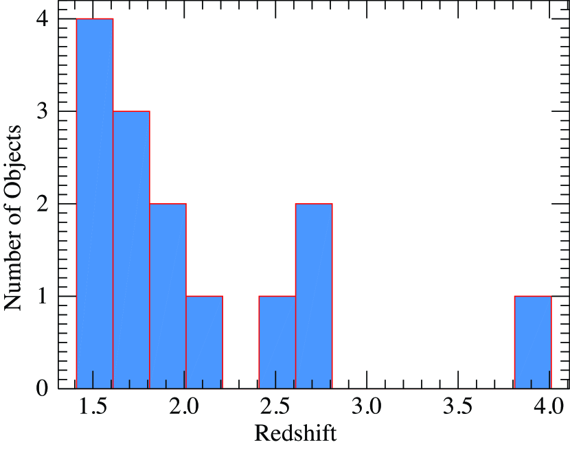
Figure 1: Redshift distribution of the quasars in our sample.

3 X-ray Observations and Data Analysis

In Table 2 we list the observation dates, exposure times and number of background-subtracted source counts of the quasars in our sample. For several objects we included published results. Specifically, for APM 08279+5255 we used the results published in Chartas et al. (2002, 2009), for HS 1700$+$6416 we incorporated the results published in Lanzuisi et al. (2012), for MG J0414+0534 we included the results from Dadina et al. (2018), for PG 1115+080 we included the results from Chartas et al. (2003, 2007) for PID352 we included the results from Vignali et al. (2015), and for the 16 Dec 2013 observation of HS 0810+2554  we used the results published in Chartas et al. (2016). For Q2237+030, Bertola et al. (2020) find significant spectral variability and indications of UFOs in several observations of this object, with outflow velocities of up to 0.5$c$. However, the main goal of the Bertola et al. (2020) study was to assess the recurrence of UFOs in this source. Since our study focuses on the physical properties of UFOs detected at high significance, we only include our recent results in the analysis. For the objects SDSS J1029$+$2623, SDSS J1529+1038, SDSS J0904$+$1512, SDSS J1353+1138, SDSS J1128+2402, SDSS J0921$+$2854, and Q2237+030 we reduced the X-ray observations using the following procedures.

For the reduction of the XMM-Newton observations we used the Science Analysis System software version 18. We filtered the pn (Strüder et al., 2001) and MOS (Turner et al., 2001) data by selecting events corresponding to instrument PATTERNS in the 0–4 (single and double pixel events) and 0–12 (up to quadruple pixel events) ranges, respectively. Moderate-amplitude background flares were present during several of the XMM-Newton observations. The pn and MOS data were filtered to exclude times when these flares occurred resulting in the effective exposure times listed in Table 2.

The contribution of the background spectra to identified absorption and/or emission features is determined by over-plotting both source and background spectra and determining the significance of the inferred spectral features while adjusting the source and background extraction regions. We note that for the Chandra spectra of the quasars in our sample the background contribution is negligible, however, the background can become comparable to the source spectra for the XMM-Newton pn spectra, especially at high energies (e.g., Chartas & Canas, 2018).

To test for sensitivity to background non-uniformity we also tried multiple background extraction regions. We did not find any differences in the spectral shapes and features using more conservative threshold cuts or selecting different background extraction regions. We selected extraction regions to optimize the S/N and ensure that the background spectra were significantly below the source spectra, especially near the energies of detected absorption lines.

The energy ranges used for fitting the pn and MOS spectra were 0.3–11 keV and 0.4–10 keV, respectively. We performed spectral fits to the pn spectra alone, and to the pn and MOS data simultaneously. Both approaches resulted in values for the fitted parameters that were consistent within the errors, however, in most cases the fits to the higher quality pn data alone yielded lower reduced $\chi^{2}$ values compared to the combined fits. We therefore consider the results from the fits to the pn data alone better suited for characterizing the properties of the X-ray absorption features. There are two exceptions where our analysis relied mostly on the MOS cameras. Specifically, for the May 2018 XMM-Newton observation of SDSS J0921 only MOS1 and MOS2 data are available. For the Oct 2018 observation of SDSS J0921 significant background flaring is present throughout the observation and the flares are much more intense in the pn than in the MOS cameras (Ebrero et al., 2020).

For the reduction of the Chandra observations we used the CIAO 4.12 software with CALDB version 4.9.1 provided by the Chandra X-ray Center (CXC). We used standard CXC threads to screen the data for status, grade, and time intervals of acceptable aspect solution and background levels. The energy ranges used for fitting the ACIS-S spectra were 0.5–8 keV.

For the gravitationally lensed sources, we extracted spectra for the combined images unless mentioned otherwise.

The extracted spectra were grouped to obtain a minimum of 20 counts in each energy bin (with the exception of Q 2237$+$0305 that was grouped to obtain a minimum of 15 counts in each energy bin), allowing use of $\chi^{2}$ statistics. This grouping was chosen for $\chi^{2}$ to be statistically valid (e.g., Cash 1979; Bevington & Robinson 2003), and to allow the maximum spectral resolution for the spectra. To further test the validity of the use of $\chi^{2}$ statistics in our analysis for our selected grouping of the data we also used the $C$-statistic (Cash 1979) on the same datasets and binned the data to have at least one count per bin. Background spectra were extracted from source-free regions.

3.1 Spectral Analysis Results

Spectra were fitted with a variety of models employing XSPEC version 12 (Arnaud, 1996). X-ray, UV, bolometric luminosities and Eddington ratios of the quasar sample are listed in Table 3. The UV luminosity densities at 1450Å were obtained from analyzing available SDSS spectra of the sampled quasars. The bolometric luminosities were calculated using two different methods: first from the X-ray bolometric correction factors and second from the luminosity density at 1450Å. Specifically, for the first method we apply a bolometric correction to the 2–10 keV luminosities based on the empirical relations presented in Duras et al. (2020). The second independent estimate of $L_{\rm Bol}$ is provided from the monochromatic luminosities at 1450$\rm\AA$ based on the empirical equations of Runnoe et al. (2012). Our independent estimates of the bolometric luminosities are very similar and show no systematic offsets. We use the difference between the two estimates to calculate the uncertainty of $L_{\rm Bol}$. The Eddington ratios use the bolometric luminosities derived from the observed optical/UV flux densities. The Eddington ratios of our sample lie in the range of 0.03 – 0.8 with a mean of 0.21 and a median of 0.15. We used the gravitational lens fitting code glafic version 1.1.6 (Oguri, 2010) to model the gravitational lens systems and obtain the magnification factors. For all spectral models we included Galactic absorption due to neutral gas (HI4PI Collaboration et al., 2016).

We proceed in fitting the following models to the data (see Tables 4, 5, and 6 ) guided by the shape and location of identified absorption and/or emission residuals:

1) power-law modified by neutral intrinsic absorption at the source.

2) power-law modified by neutral intrinsic absorption and a number of absorption and/or emission lines.

3) power-law modified by neutral intrinsic absorption, outflowing intrinsic ionized absorption and an emission line if required.

For the outflowing ionized absorber we used the XSTAR photoionization model warmabs (Kallman & Bautista, 2001; Kallman et al., 1996). For improved accuracy and flexibility we use the analytic XSTAR versions of the warmabs model instead of the XSTAR table models. Our XSTAR warmabs model assumes a spherical, constant density photo-ionized outflowing optically thin absorber with a source at its center.

The default atomic population file pops.fits provided in NASA’s warmabs distribution uses a fixed value of the photon index of $\Gamma$ = 2. However, our spectral analysis indicates that the photon index $\Gamma$ differed from this default value for most observations of our quasar sample. We therefore used XSTAR to create new population files appropriate for photon indices of each observation.

We model the velocity broadening of the absorption lines by introducing in the XSTAR models large turbulent velocities. Several mechanisms may lead to velocity broadening, including velocity gradients along the radial direction of motion (e.g., Schurch & Done, 2007; Saez & Chartas, 2011; Fukumura et al., 2018), and velocity gradients along a transverse direction of motion of plasma around the black hole corona (e.g., Fukumura & Tombesi, 2019). We propose additional explanations, such as relativistic effects, that may be important for outflows launched near the ISCO, and variability of the velocity of the outflow over timescales shorter than the total exposure time. The spectra presented here, however, do not have adequate S/N and/or spectral resolution to distinguish between these possible mechanisms. We performed several fits where we allowed the turbulent velocity to vary and found the best-fit values. Because of the low to moderate S/N of the Chandra and XMM-Newton spectra, the turbulent velocities, are not well constrained. For the error analysis of the remaining variables in spectral fits that used the XSTAR model we froze the turbulent velocities at the best-fit values and list these values in Tables 4, 5, and 6.

In Figure 2 we show the UV and X-ray spectra of the sources where significant ultrafast outflows are shown, and have not been previously published. The UV spectra (left column) show the CIV broad emission lines and blueshifted absorption lines indicative of outflows with velocities of up to 0.075$c$. The X-ray spectra (middle column) show highly blueshifted absorption lines which are occasionally accompanied by emission lines (P-Cygni profiles), indicative of ultrafast outflows with non-negligible (or large) covering factors. The emission line in a P-Cygni feature is thought to be produced by fluorescence from the entire outflow, whereas the expanding outflow along our line-of-sight produces the blueshifted absorption line. We find that the X-ray spectra of 5(3) of the 14(6) quasars in our sample(subsample) contain P-Cygni profiles. The energies and equivalent widths of the emission lines in these P-Cygni profiles indicate that they do not originate from reflection from the accretion disk or distant cold matter such as a molecular torus. Specifically, the energies of the detected emission lines in the P-Cygni profiles detected in our sample lie in the range of $6.6-11.7$ keV and their equivalent widths lie in the range of $0.75-2.3$ keV. Conversely, studies of the X-ray spectra of quasars (e.g., Inoue et al., 2007; de La Calle Pérez et al., 2010) indicate that a large fraction of them contain emission lines due to reflection with energies of $\sim$ 6.4 keV and with equivalent widths that lie in the range of $130-280$ eV.

The confidence levels (right column) of the ultrafast outflow detections, calculated using $\chi^{2}$ and $\sl Cash$ statistics are found to be $>$ 99%, with the exception of SDSSJ0904 that is detected with a significance of $>$ 90% confidence. We emphasize that these results are independent of the statistic used in the analysis of the spectra. In particular, the absorption and emission line parameters are always consistent (within the 68% confidence level) using the $\sl Cash$ or the $\chi^{2}$ statistic (see Figure 2).

We followed a more robust approach of estimating the significance of the blueshifted absorption and emission lines in the X-ray spectra based on Monte Carlo simulations to determine the distribution of the F-statistic between models (Protassov et al., 2002). We considered a null model that included a simple absorbed power law and an alternative model that in addition included one or two Gaussian absorption and/or emission lines. For each observed spectrum we simulated 1000 data sets using the XSPEC fakeit command. We fit the null and alternative models to the 1000 simulated data sets and computed the $F$-statistic for each fit. We computed the probability, $P_{F\rm}$, for the F value to exceed the value determined from the fits of the null and alternative models to the observed spectra. The probabilities $P_{\rm F}$ for all objects are listed in Tables 4, 5, and 6 and are found to be $<$0.01 with the exception of SDSSJ0904 for which $P_{\rm F}$ = 0.035.

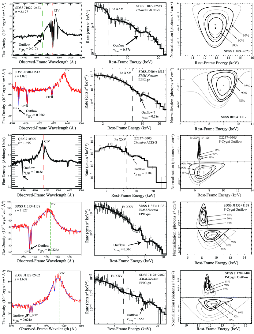
Figure 2: The UV and X-ray spectra of the sources for which the X-ray spectra have not been previously published with claimed ultrafast outflows. (left) Rest-frame UV spectra showing NALs. The spectrum of Q2237 is adapted from O’Dowd et al. (2011). (middle) X-ray spectra showing blueshifted absorption lines. (right) confidence contours of the absorption and/or emission lines of the ultrafast outflows. Black and thick contours are based on spectral fits that use ${\chi}^{2}$ statistics and grey and thin contours are based on spectral fits that use $Cash$ statistics.

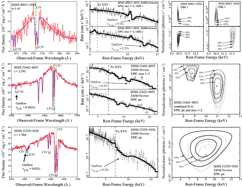
Figure 2 (Cont.): The UV and X-ray spectra of the sources for which the X-ray spectra have not been previously published with claimed ultrafast outflows. (left) Rest-frame UV spectra showing NALs. (middle) X-ray spectra showing blueshifted absorption lines. (right) confidence contours of the absorption and/or emission lines of the ultrafast outflows. Black and thick contours are based on spectral fits that use ${\chi}^{2}$ statistics and grey and thin contours are based on spectral fits that use $Cash$ statistics.

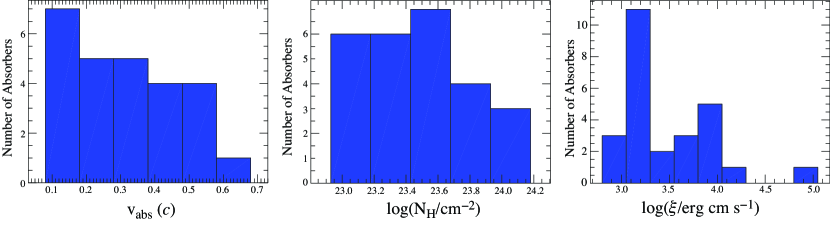
Figure 3: Distributions of the velocities, absorber column densities, and ionization parameters of our sample of high-$z$ quasars.

Due to an operational problem, only MOS 1,2 data were obtained during the XMM-Newton observation of SDSSJ0921 in May 2018. The observation of SDSSJ0921 was rescheduled in Oct 2018 during which both EPIC pn and MOS 1,2 data were obtained. In Figure 2 we show the variability of the outflow in SDSSJ0921 between the two observations. The projected velocity of the outflow along our line of sight has increased from 0.41$c$ to 0.53$c$ between observations. The outflow is detected at the same velocity in both the MOS12 and pn spectra of the Oct 2018 observation. The emission line detected in SDSSJ0921, which possibly originates from iron fluorescence from the entire outflow, shows no significant change in energy between the two observations. The XMM-Newton observation of SDSSJ1442 was also significantly affected by flares and the background was especially elevated in the pn detector. Two blueshifted absorptions lines are detected in both MOS 1+2 and pn spectra of SDSSJ1442 indicating an outflow with two velocity components.

We also detect an emission line with a rest-frame energy of $\sim$16.44 keV in the spectrum of SDSSJ1442. The 16.44 keV line is detected at the $>$ 99% confidence level and our Monte Carlo simulations confirm it to be significant ($>$ 99.9% confidence level) and not a random fluctuation. We interpret the large energy shift of the line with respect to the energy of the expected Fe K$\alpha$ fluorescence line as possibly being the result of microlensing in one of the lensed images of SDSS J1442. Similar blueshifted lines have been detected in several lensed quasars (e.g., Chartas et al., 2017). Future observations with the Chandra X-ray Observatory would be required to resolve the spectra of the images to confirm the microlensing interpretation.

In Figure 3 we show the distributions of the velocities, absorber column densities, and ionization parameters of the outflowing X-ray absorbers of our sample. These outflow properties are taken from spectral fits with models that incorporate the outflowing photoionized absorber listed as model 3 in Tables 4, 5, and 6. Several of the objects in our sample were observed over multiple epochs (see Table 2) and several of the objects contained multiple outflowing absorbers. The projected values of the outflow velocities of the absorber lie in the range of $\sim$ 0.1$-$0.6$c$, the absorber column densities lie in the range of $\sim$ 9 $\times$ 10²² $-$ 1 $\times$ 10²⁴ cm^-2, and the ionization parameters lie in the range of $\sim$ 10^2.8 $-$ 10⁵ erg cm s^-1.

3.1.1 Energetics of Quasar Outflows

For estimating the energetics of the wind we assume a spherically symmetric outflow with a covering factor of $f_{\rm c}$ (e.g., Lamers & Cassinelli, 1999). We approximate the hydrogen column density $N_{\rm H}\sim n(r){\Delta}r$, where $n(r)$ is the number density (particles cm^-3) of the gas at radius $r$. We use the following expressions to estimate the mass-outflow rate (equation 1), the kinetic power (equation 2), and the rate of change of momentum of the outflow (equation 3):

$$\dot{M}=4{\pi}r(r/{\Delta}{r})N_{\rm H}m_{\rm p}v_{\rm wind}f_{\rm c}$$ (1)

$$\dot{E}_{\rm K}={{1}\over{2}}{\dot{M}{v^{2}_{\rm wind}}}$$ (2)

$$\dot{{p}}=\dot{{M}}v_{\rm wind}$$ (3)

where ${\Delta}{r}$ is the thickness of the absorber at radius $r$, $N_{\rm H}$ is the hydrogen column density, $v_{\rm wind}$ is the outflow velocity of the X-ray absorber, and $f_{\rm c}$ is the global covering factor of the absorber.

We used a Monte Carlo approach to estimate the errors of $\dot{M}$, $\dot{E}$${}_{\rm K}/L_{\rm Bol}$, and $\dot{p}/(L_{\rm Bol}/c)$. The values of $v_{\rm wind}$, $N_{\rm Habs}$, $M_{\rm BH}$, and $L_{\rm Bol}$ were assumed to have normal distributions within their error limits. The values of $f_{\rm c}$, $r/{\Delta}{r}$, and $r$ were assumed to have uniform distributions within their error limits. By multiplying these distributions and with the appropriate constants from equations 1, 2, and 3 we obtained the distributions of $\dot{M}$, $\dot{E}$${}_{\rm K}/L_{\rm Bol}$, and $\dot{p}/(L_{\rm Bol}/c)$. We finally determined the mean values of the distributions of $\dot{M}$, $\dot{E}$${}_{\rm K}/L_{\rm Bol}$, and $\dot{p}/(L_{\rm Bol}/c)$ and estimated the 68% confidence ranges.

Special relativistic effects in modeling ultrafast outflows were recently presented in Luminari et al. (2020). As a consequence of these relativistic effects the true hydrogen column densities of the outflowing absorbers are larger than the observed column densities by a velocity depended factor. In Table 9 we list the relativistic correction factors as calculated in Luminari et al. (2020) for the observed outflow velocities. The mass-outflow rate, the kinetic power, and the rate of change of momentum of the outflow are all proportional to the column density and therefore these quantities also need to be adjusted by the relativistic correction factor.

The locations of the absorbers is not well constrained with the available CCD resolution spectra. As a conservative approach (see Gofford et al., 2015) we calculate a lower bound of the distance of the absorber from the center of the black hole, $r_{\rm min}$, by equating the observed velocity with the escape velocity at that radius.

$$r_{min}=R_{s\rm}(c/v_{\rm wind})^{2},$$ (4)

where $v_{wind}$ is the observed outflow velocity and $R_{\rm s}$ = $2GM/c^{2}$, is the Schwarzschild radius. We note that we observe the projected component of the wind velocity. The true outflow velocity will be larger than the observed one and the true radius will be smaller than this $r_{\rm min}$ value depending on the angle between our line of sight through the absorber and the velocity of the X-ray absorbing material. The observed wind velocities are derived from the best-fit redshift parameters $z_{\rm abs}$ of model 3 in Tables 4, 5, and 6, where the outflowing ionized absorber is modeled with the photoionization software package XSTAR.

Variability of the properties of the ultrafast outflows has been observed and reported in several quasars of our sample including APM08279, PG1115, and HS1700 on timescales comparable to the light crossing time over regions of 10$-$100$r_{\rm g}$ (Chartas et al., 2003, 2009; Saez & Chartas, 2011; Lanzuisi et al., 2012). The short term variability timescale of the X-ray absorption lines suggest that the distances of the outflowing absorbers from the center of the black holes are consistent with the estimates of $r_{\rm min}$.

In the case that the wind is not continuous but made up of clouds we can define a filling factor $f=V_{\rm gas}/V$. Assuming the clouds have a thickness of ${\Delta}r$, the column density is ${N}_{\rm H}\sim n(r)(\Delta r)f$ and the distance between the ionizing source and the absorbing cloud is given by

Figure 4: Distribution of the distances of the ionized ultrafast absorbers from the central sources of our quasar sample.

$${{r}_{\rm absorber}=\left(\frac{{L}_{ion}\Delta rf}{\xi{N}_{H}}\right)}^{1/2}$$ (5)

In order to obtain an upper limit on the location of the absorber, the following approximations are often used in the literature, ${\Delta}r/r$ = 1 and a filling factor of $f$ = 1 (e.g., Tombesi et al., 2012; Gofford et al., 2015). These approximations lead to the following upper limit on the location:

$${r}_{\rm max}=\frac{{L}_{ion}}{\xi{N}_{H}}$$ (6)

Figure 5: Left: Distribution of the fraction of the kinetic luminosity to the bolometric luminosity ($\dot{E}$${}_{\rm K}/L_{\rm Bol}$) of the ultrafast absorbers of our high-$z$ quasar sample (left-bottom), of the low-$z$ Gofford sample (left-top), and of the low-$z$ Tombesi sample (left-middle). Right: Distribution of the momentum boost ($\dot{p}/(L_{\rm Bol}/c)$) of the ultrafast absorbers of our high-$z$ quasar sample (right-bottom), of the low-$z$ Gofford sample (right-top), and of the low-$z$ Tombesi sample (right-middle). For objects with multiple observations the average values are displayed. No relativistic correction is applied to the outflow efficiency and momentum boost.

Figure 6: Left: Distribution of the fraction of the kinetic luminosity to the bolometric luminosity ($\dot{E}$${}_{\rm K}/L_{\rm Bol}$) of the ultrafast absorbers of our high-$z$ quasar sample (left-bottom), of the low-$z$ Gofford sample (left-top), and of the low-$z$ Tombesi sample (left-middle). Right: Distribution of the momentum boost ($\dot{p}/(L_{\rm Bol}/c)$) of the ultrafast absorbers of our high-$z$ quasar sample (right-bottom), of the low-$z$ Gofford sample (right-top), and of the low-$z$ Tombesi sample (right-middle). For objects with multiple observations the average values are displayed. A relativistic correction is applied to the outflow efficiency and momentum boost.

There are several problems with using ${r}_{\rm max}$ with ${\Delta}r/r$ = 1 and $f=1$ as a useful upper limit for the location of the absorber. Filling factors based on estimates for absorbing clouds can be as small as $\sim$ 1 $\times$ 10^-6 (e.g., Laha et al., 2016) . Assuming $f=1$ and ${\Delta}r=r$ can result in estimated ${r}_{\rm max}$ values that are several orders of magnitude larger than the true values of ${r}_{\rm absorber}$. Using Equation 6 will also result in an overestimate of quantities that are proportional to ${r}_{\rm absorber}$ such as the mass-outflow rate, the outflow efficiency and the momentum boost. In Table 9 we list the ratio of $r_{\rm max}/r_{\rm min}$. For our study we are interested in placing conservative constraints on the energetics of ultrafast outflows and determining whether they are powerful enough to produce feedback on their host galaxies based on criteria presented in Hopkins et al. (2016). We therefore adopt the $r_{\rm min}$ values for estimating the location of the absorbers resulting in lower limits of the energetics of the outflows.

In Table 9, we list the total hydrogen column densities $N_{\rm H}$ of the X-ray absorption lines, the relativistic corrections of the optical depths, the minimum and maximum distances between the ionizing source and the absorbing cloud, the ionization parameters, the outflow velocities of each absorption component, the mass-outflow rates, the efficiency of the outflows and the momentum boosts of the outflows. In Figure 4 we present the distribution of the estimated $r_{\rm min}$ values of the quasars of our sample derived from Equation 4. Most quasar winds appear to have $r_{\rm min}$ $\,\buildrel\scriptstyle<\over{\scriptstyle\sim}\,$ 100$~{}r_{\rm g}$, with a significant fraction have $r_{\rm min}$ near $\sim$ 20$~{}r_{\rm g}$. This is consistent with detailed general-relativistic radiative magneto-hydrodynamic (GR-rMHD) simulations, showing a continuous production of fast AGN outflows within such a micro-scale region (e.g., Sadowski & Gaspari, 2017).

Insight into the acceleration mechanism of ultrafast outflows is obtained by estimating the fraction of their kinetic luminosity ($\dot{E}$_K) to the bolometric luminosity ($L_{\rm Bol}$). An efficiency fraction, $\dot{E}$${}_{\rm K}/L_{\rm Bol}$ near or greater than the covering fraction would imply that a driving mechanism in addition to radiation pressure must be contributing to the acceleration of ultrafast outflows. Specifically, assuming that the bolometric emission of the high-$z$ sample is approximately isotropic, an outflowing wind with a covering fraction of $f_{\rm c}$ will at most receive a fraction $f_{\rm c}$ of the total bolometric luminosity.

The global covering factor of the absorber is often estimated from modeling the P-Cygni profile of the outflowing spectral feature or from the observed fraction of AGN that show ultrafast outflows in their X-ray spectra. Many of the available P-Cygni models used to fit the X-ray spectra of ultrafast quasar winds (e.g., windabs) ignore the presence of the accretion disk and do not include general relativistic effects that are expected to be important for winds launched near the event horizon. Dorodnitsyn (2009) has simulated P-Cygni profiles produced in the vicinity of quasars, taking into account Doppler and gravitational effects. These simulations indicate that current models that do not include general relativistic effects and an accretion disk are crude approximations and will result in unreliable constraints on the geometry of the wind. We therefore assume a global covering factor of $f_{c}$ = 0.4 with the knowledge that current observations suggest that about 40% of nearby AGN contain ultrafast outflows (e.g., Tombesi et al., 2010; Gofford et al., 2013). In Figures 5 and 6 we show the distributions of the efficiency fraction $\dot{E}$${}_{\rm K}/L_{\rm Bol}$ and momentum boost for our high-$z$ sample without and with relativistic corrections (wrc), respectively. About 64% (86% wrc) of the high-$z$ sample have $\dot{E}$${}_{\rm K}/L_{\rm Bol}$ $\,\buildrel\scriptstyle>\over{\scriptstyle\sim}\,$ 0.4 and about 86% (100% wrc) have $\dot{p}/(L_{\rm Bol}/c)$ $\,\buildrel\scriptstyle>\over{\scriptstyle\sim}\,$ 1. As a comparison, from the low-$z$ Tombesi sample (see Figures 5 and 6) we find that about 20% (20% wrc) of local AGN have $\dot{E}$${}_{\rm K}/L_{\rm Bol}$ $\,\buildrel\scriptstyle>\over{\scriptstyle\sim}\,$ 0.4 and about 40% (50% wrc) of them have $\dot{p}/(L_{\rm Bol}/c)$ $\,\buildrel\scriptstyle>\over{\scriptstyle\sim}\,$ 1. For the comparison of the low and high-$z$ AGN samples we have assumed the minimum estimates of $\dot{E}$_K that assume the distance to the absorber is given by equation 4.

Finally, the retrieved high mechanical feedback power ratio (Figures 5 and 6, left) is a clear signature that the micro/meso AGN feedback will have a substantial impact on the evolution of the host hot halos estimated to have $T_{\rm x}\sim 1-2$ keV (Gaspari et al., 2019).

Figure 7: Velocity-aligned normalized flux profiles of detected C IV transitions in NAL systems towards SDSSJ1529, SDSSJ0904, SDSS J1353, and SDSS J1128. The blue and red components of the doublet are shown with the blue and red histograms, respectively. The bottom lines show the normalized 1 $\sigma$ errors. The coverage fractions evaluated over the central region of the absorption lines are plotted with filled black circles.

4 UV Observations and Data Analysis of Subsample

The UV spectra of our subsample of six quasars were taken with the Sloan Digital Sky Survey. Processed and calibrated spectra were downloaded from the SDSS database. We analyzed each spectrum with a multicomponent fitting code written in Python. Each spectrum was corrected for Galactic extinction using the Schlafly & Finkbeiner (2011) map and a Milky Way extinction law of Fitzpatrick & Massa (1999) with a reddening parameter of $R_{\rm V}=3.1$. The flux densities were corrected for the gravitational lens magnifications listed in Table 2. The model fitting function used has the form:

$${f}_{\lambda}=a+b\lambda+\sum_{i=1}^{i=N}{\frac{1}{\sigma\sqrt{2\pi}}}{e}^{-\frac{1}{2}\frac{{\left(\lambda-\mu\right)}^{2}}{{\sigma}^{2}}}$$ (7)

The model function was fit to the SDSS spectra using the non-linear least squares Python routine scipy.optimize.curve_fit. The region of interest of the fit covers the C IV emission line and all significant absorption lines blueward of the emission line. The C IV $\lambda\lambda$1548.19,1550.77 doublet ratio is often used to constrain the coverage fraction $C(v)$ and optical depth $\tau(v)$ of the absorbing material in front of the emission source (e.g., Hamann et al., 1997; Hamann & Sabra, 2004). The doublet method of estimating the coverage fraction assumes that the outflowing UV absorbing gas is spatially homogeneous in front of a spatially uniform emission source. The normalized flux densities across the blue and red components of the doublet, assuming a coverage fraction $C(v)$, are given by the following expressions:

$${I}_{B}\left(v\right)=\left(1-C\left(v\right)\right)+C\left(v\right){e}^{-2\tau(v)}$$ (8)

$${I}_{R}\left(v\right)=\left(1-C\left(v\right)\right)+C\left(v\right){e}^{-\tau(v)}$$

The solutions to these two equations provide the coverage fraction $C(v)$ and the optical depth $\tau(v)$ as a function of velocity. A coverage fraction of less than one indicates that the absorber is likely intrinsic and associated with an outflowing wind from the quasar (e.g., Misawa et al., 2007; Itoh et al., 2020). Intervening absorbers and foreground galaxies have angular sizes considerably larger than the central sources and would produce coverage fractions of $\sim$ 1.

In Table 7 we list the central wavelengths and FWHM of the detected blueshifted absorption lines. We also provide the outflow velocities of the blue-shifted absorption lines. We find at least one blueshifted C IV doublet component in each quasar of the subsample. The FWHM values of all blueshifted C IV absorption lines in the subsample are $<$ 500 km s^-1. Based on these velocity widths we classify the blueshifted absorption lines in the subsample as NALs. In Table 8 we list the equivalent widths of the absorption lines, the coverage fraction $C(v)$, the optical depth $\tau(v)$ averaged over the central region of the absorption lines, and the C IV ionic column density. Several of the absorption line depths are either very shallow in the C IV doublet or the red component has a slightly larger depth than the blue one within the error bars. In these cases the doublet method yields unphysical values for several velocity bins and we cannot provide estimates for $C_{\rm f}$, $\tau$ and $N_{\rm CIV}$. We find that 4 of the 6 quasars of the subsample contain an outflowing component with a coverage fraction less than 1 indicating that they are likely intrinsic. For the two quasars J1442 and J0921, where we cannot constrain the coverage fraction, we find that they contain C IV doublets with outflow velocities of $\sim$12,700 km s^-1 and $\sim$ 5,160 km s^-1, respectively. These absorbers are possibly also intrinsic since these outflow speeds are too high for the absorbers to be environmental gas and NAL systems with velocity separations between 3,000 and 12,000 km s^-1 are found to be dominated by absorbers intrinsic to and outflowing from the quasar (e.g., Stone & Richards, 2019).

We conclude, that based on our estimated coverage fractions and outflow velocities, all the quasars of our subsample contain outflows of UV absorbing gas with velocities ranging between 5,160 km s^-1 and 22,740 km s^-1.

We have assumed Gaussian optical depth profiles which leads to the following simplified approximation of the ionic C IV column density (e.g., Moravec et al., 2017):

$${N}_{CIV}=6.68\times{10}^{14}\left(\frac{b{\tau}_{0,R}}{{f}_{R}{\lambda}_{0,R}}\right){cm}^{-2},$$ (9)

where $\lambda_{\rm 0,R}$ = 1550.77 Å is the laboratory wavelength of the redder transition of the C IV doublet, $f_{\rm R}$ is the line oscillator strength of the $\lambda_{\rm 0,R}$ transition of the doublet, $b$ is the Doppler parameter with units of km s^-1, and $\tau_{\rm 0,R}$ is the line-centre optical depth of the redder transition of the C IV doublet.

The spectral resolution of the SDSS spectra (1500 at 3800 Å) is insufficient to resolve the C IV absorption profiles and many of the absorption lines appear to be saturated. As a result, our estimated values of the ionic column densities of the absorbers listed in Table 8 should be considered as lower limits.

C IV $\lambda\lambda$1548.19,1550.77 doublets have intrinsic optical depth ratios of $\sim$ 2:1. The observed line depth ratios of $\sim$ 1:1 in most doublets of our subsample indicate strong saturation, partial covering and large optical depths (e.g., Hamann et al., 2019). Saturation may lead to significant underestimates of the column densities of the outflowing UV absorbing gas and estimates of the ionization parameter in these cases are also unreliable. We have thus not attempted to constrain the energetics of the outflowing UV absorbing gas with the available SDSS spectra.

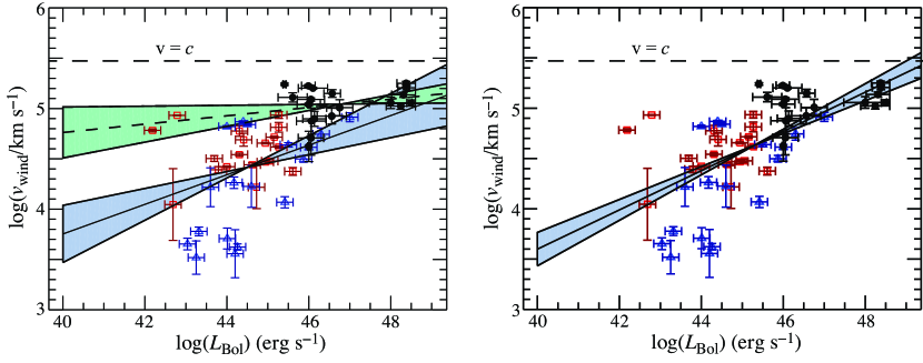
Figure 8: The outflow velocity of the ionized absorber versus bolometric luminosity of the low-$z$ Tombesi (red squares), low-$z$ Gofford (blue triangles) and high-$z$ (black filled circles) AGN samples. (left) We show the power-law least-squares fits to the combined Tombesi and Gofford samples with the solid line and to the high-$z$ sample with the dashed line. (right) We show the power-law least-squares fits to the combined Tombesi, Gofford and high-$z$ samples with the solid line. The shaded areas represent the uncertainty of the slopes of our fits to the data.

5 Discussion

We searched for a possible correlation between the outflow velocity, $v_{\rm wind}$, of X-ray absorbing gas and the bolometric luminosity, $L_{\rm Bol}$, of AGN. We considered three different AGN samples for our $v_{\rm wind}-L_{\rm Bol}$ correlation analysis. The first sample includes the high-$z$ quasars of our study, with bolometric luminosities and velocities taken from Tables 3 and 9, respectively. For quasars APM08279, PG1115, HS0810, and SDSSJ1442 that contain two velocity components in the same observation, the largest velocity component is considered in the $v_{\rm wind}-L_{\rm Bol}$ correlation analysis. The second sample (referred to as the Tombesi sample) contains the 12 type-1 AGN and 3 type-2 AGN listed in Table 1 of Tombesi et al. (2012). The redshifts of the AGN in the Tombesi sample range between 0.00233 and 0.1040. The third comparison sample (referred to as the Gofford sample) includes 15 of the 20 AGN listed in Table 1 of Gofford et al. (2015). For the Gofford sample we excluded APM08279 because it is a high-$z$ quasar that is included in our high-$z$ sample, we excluded NGC 3783 and NGC 4395 because their outflow velocities are not constrained, and we excluded MCG-6-30-15 and NGC 3516 because their low outflow velocities and relatively low column densities place them close to the warm absorber category of winds. The Gofford sample is comprised of 3 BLRGs, 9 type-1 AGN and 3 type-2 AGN. The redshifts of the AGN in the Gofford sample range between 0.00234 and 0.18. In cases where multiple observations of an object are available, the outflow velocities and corresponding bolometric luminosities of the individual observations are considered for our analysis of the $v_{\rm wind}-L_{\rm Bol}$ data and not the average of these quantities over the observations.

The outflows in the three samples considered for our analysis of the $v_{\rm wind}-L_{\rm Bol}$ data are associated with outflowing absorbers that have ionization parameters larger than $\log(\xi/\rm erg~{}cm~{}s^{-1})=3$, hydrogen column densities larger than $\log(N_{\rm H}/\rm cm^{-2})=22$ and outflow velocities larger than 3,000 km s^-1. We are not considering outflows commonly associated with warm absorbers that have ionization parameters in the range $\log(\xi/\rm erg~{}cm~{}s^{-1})=-1$ to 3, column densities in the range $\log(N_{\rm H}/\rm cm^{-2})$ = 20–22 and outflow velocities in the range $v$ = 100–2,000 km s^-1 (e.g., Laha et al., 2014). We note that the analysis presented in Tombesi et al. (2010, 2012) included outflowing absorbers with velocities above 10,000 km s^-1.

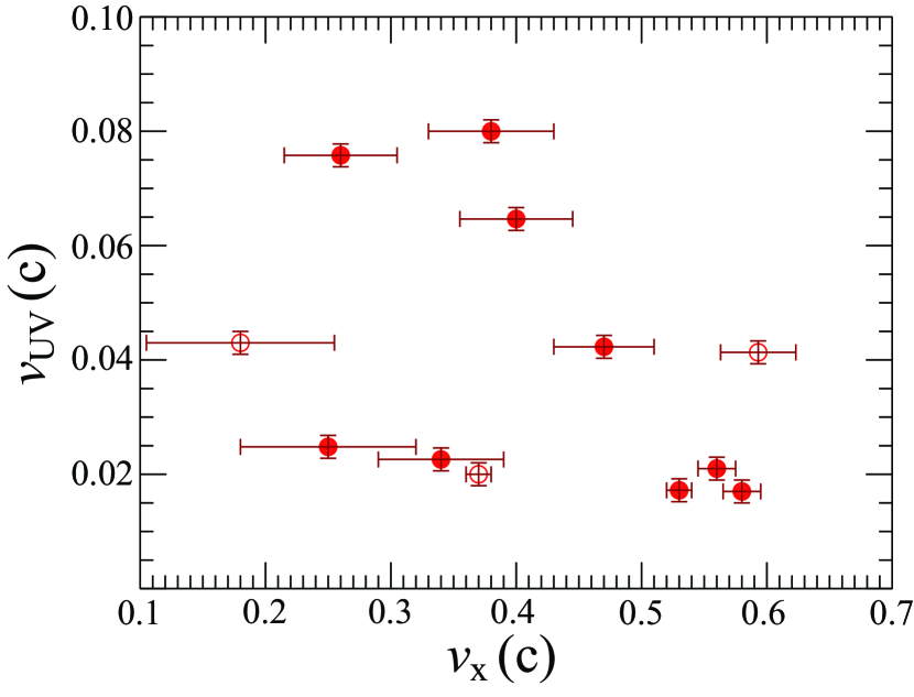
Figure 9: The X-ray and UV velocities of the outflowing ionized absorbers of the high-$z$ quasar sample. The NAL quasars are shown with filled red circles and the rest of the sample with open red circles. No significant correlation is found for the entire sample, however, a possible anti-correlation is found for the NAL quasar sample.

In Figure 8 we show the outflow velocities of our high-$z$ AGN sample (in black), the Tombesi low-$z$ sample (in red) and the Gofford low-$z$ sample (in blue) as a function of bolometric luminosity. For a radiation-driven outflow we expect $v_{wind}$ $\propto$ $L^{1/2}$ (e.g., see equation 1 of Chartas et al., 2002). For the fits to the low-$z$ Tombesi and Gofford samples we find best-fit values of the power-law exponents of $b=0.02\pm 0.06$ and $b=0.29\pm 0.09$, respectively. We find a Kendall’s rank correlation coefficient of $\tau$ = 0.1 with a null probability of $P_{\rm null}$ = 0.52 for the low-$z$ Tombesi sample and $\tau$ = 0.45 with a null probability of $P_{\rm null}$ = 8.9 $\times$ 10^-3 for the low-$z$ Gofford sample. We conclude that the low-$z$ Gofford AGN sample shows a strong and significant correlation between $v_{\rm wind}$ and $L_{\rm Bol}$, in agreement with the result first presented in Gofford et al. (2015), whereas no correlation between $v_{\rm wind}$ and $L_{\rm Bol}$ is found for the low-$z$ Tombesi sample. One possible explanation for this difference it that Tombesi et al. (2012) did not include outflows with velocities between 3,000 and 10,000 km s^-1.

For the fit to our high-$z$ quasar sample we find a best-fit value of the power-law exponent of $b=0.03\pm 0.06$. We find a Kendall’s rank correlation coefficient of $\tau$ = 0.1 with a null probability of $P_{\rm null}$ = 0.55 for the high-$z$ AGN data. For the combined fit to the low-$z$ Tombesi and Gofford samples and our high-$z$ quasar sample we find a best-fit value of the power-law exponent of $b=0.20\pm 0.03$, significantly below the value predicted for radiation driving alone. We find that the fit to the combined samples results in a Kendall’s rank correlation coefficient of $\tau$ = 0.51 with a null probability of $P_{\rm null}$ = 6 $\times$ 10^-8.

In Table 10 we list the correlation coefficients and best-fit power-law exponents for our analysis of the $v_{\rm wind}-L_{\rm Bol}$ data of the low-$z$ Tombesi and Gofford samples and our high-$z$ quasar sample. The best-fit value of $b=0.15\pm 0.06$ for the combined low-$z$ Tombesi and Gofford samples is also below what would be predicted for radiation driving for the acceleration of accretion disk winds at low-$z$. The high-$z$ AGN sample alone shows higher outflow velocities and no significant dependence between outflow velocities and bolometric luminosity suggesting that an additional driving mechanism may be contributing to the outflow. Another possibility for the non-dependence between luminosity and outflow velocity for the most luminous objects is that there is a saturation effect in the acceleration process for velocities $\,\buildrel\scriptstyle>\over{\scriptstyle\sim}\,$ 0.1$c$ due to relativistic beaming (e.g., Schurch & Done, 2007; Saez & Chartas, 2011; Luminari et al., 2020).

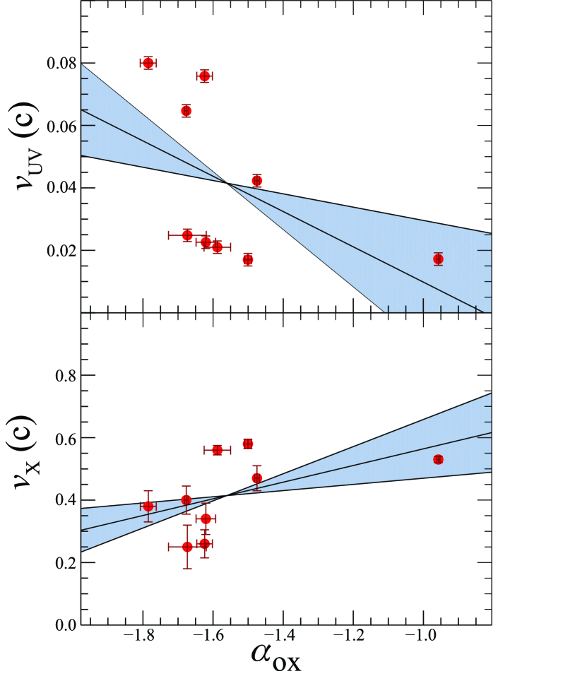
Figure 10: The UV (top) and X-ray (bottom) velocities of the outflowing ionized absorbers of the high-$z$ NAL quasars of our sample as a function of the optical-to-X-ray spectral index $\alpha_{\rm ox}$. The solid lines represent the fits to the data and the shaded areas represent the uncertainty of the slopes of our fits to the data.

In Figure 9 we show the maximum velocities of the UV and X-ray outflowing absorbers of our high-$z$ sample. By including all the quasars in our sample we find no significant correlation between UV and X-ray velocities. If we only include the NAL quasars (see classification in Table 1) we find a possible anti-correlation between the maximum UV and X-ray outflow velocities with Kendall’s rank correlation coefficient $\tau$ = $-$0.5 significant at $>$ 94%. To obtain some insight as to the origin of this possible anti-correlation between $v_{\rm UV}$ and $v_{\rm X}$ we calculate the optical-to-Xray spectral slopes ($\alpha_{\rm ox}$ ) of the NAL quasars of our sample. Several theoretical studies have demonstrated that the spectral energy distribution of the incident flux on the absorbing gas may significantly influence the dynamics of the outflow (e.g., Saez & Chartas, 2011; Krawczyk et al., 2013). We therefore predict, based on these studies, that the optical-to-X-ray spectral slopes of the NAL quasars of our sample may affect the acceleration of the outflowing absorbers.

In Table 11 we list the rest-frame 2 keV and 2500 Å  flux densities and the calculated $\alpha_{\rm ox}$ values of the NAL quasars. In Table 11 we also list the quantity $\Delta\alpha_{\rm ox}$ that represents the difference between the observed value of $\alpha_{\rm ox}$ and the value expected based on the UV luminosity of the quasar (e.g., Lusso et al., 2010). In all NAL quasars of our sample $\Delta\alpha_{\rm ox}$ is relatively small with the exception of SDSSJ0921 with $\Delta\alpha_{\rm ox}$ $\sim$ 0.5. SDSSJ0921 is not significantly absorbed in the X-ray band and the positive value of $\Delta\alpha_{\rm ox}$ suggests absorption in the UV band.

The X-ray and optical flux densities are corrected for Galactic absorption. We find that the UV outflow velocities are weakly anti-correlated with $\alpha_{\rm ox}$ (Kendall’s rank correlation coefficient of $\tau$ = $-0.61$ and null probability of $P$ = 0.02) and the X-ray outflow velocities are weakly correlated with $\alpha_{\rm ox}$ (Kendall’s rank correlation coefficient of $\tau$ = $0.44$ and null probability of $P$ = 0.09). In Figure 10 we show $v_{\rm UV}$ and $v_{\rm X}$ as a function of $\alpha_{\rm ox}$. These trends are suggestive of a possible dependence of the UV and X-ray outflow velocities on the slope of the incident spectral energy distribution and are consistent with an anti-correlation between the maximum UV and X-ray outflow velocities. The outflows of UV absorbing gas appear to be accelerated to larger velocities in the X-ray-weak NAL quasars of our sample and the outflows of X-ray absorbing gas appear to be accelerated to larger velocities in the X-ray-strong NAL quasars. We caution that the current sample size is relatively small and the correlations between outflow velocities and $\alpha_{\rm ox}$ for our sample of NAL quasars are weak. A significant increase of a factor of at least two will be required to confirm these results.

We find no significant correlations between the observed properties of UFO velocity, column density, ionization parameter, bolometric luminosity, X-ray luminosity, and Eddington ratio in the high-$z$ quasar sample. Conversely, correlations between $v_{\rm wind}$ versus $L_{\rm X}$ have been reported in individual quasars such as $z=3.91$ APM 08279$+$5255 (Chartas et al., 2002, 2009; Saez & Chartas, 2011), $z=0.184$ PDS 456 (Nardini et al., 2015; Matzeu et al., 2017; Reeves et al., 2018), $z=0.062$ PG 1126$-$041 (Giustini et al., 2011) and $z=2.7348$ HS 1700+6416 (Lanzuisi et al., 2012). A plausible explanation for this apparent discrepancy is that the outflow velocities of high-$z$ quasars may depend more strongly than low-$z$ AGN on additional driving mechanisms, such as magnetic pressure, and this dependance may vary between quasars. GR-rMHD simulations (e.g., Sadowski & Gaspari, 2017) show that both radiative and magnetic driving contribute to accelerating ultrafast outflows.

One possible test of this hypothesis is finding and comparing possible individual correlations between $v_{\rm wind}$ versus $L_{\rm X}$ of quasars in this sample. This test is not yet feasible with the available data. Differences in the $v_{\rm wind}$ versus $L_{\rm X}$ correlations of individual objects may lead to a dilution of a single significant correlation in the entire sample. In support of the presence of a driving mechanism in addition to radiation driving are the observed large fractions of the kinetic luminosity to the bolometric luminosity of the high-$z$ quasars. As reported in Table 9 (column 7), ten out of the fourteen quasars in the sample have fractions of the kinetic luminosity to the bolometric luminosity greater that 0.4, which is not consistent with radiation driving.

Variability of the properties of the ultrafast outflows has been observed and reported in several quasars of our sample including APM08279, PG1115, HS1700, Q2237, and HS0810 on timescales comparable to the light crossing time over regions of 10$-$100 $r_{\rm g}$. In APM08729 we found a strong correlation between the maximum outflow velocity and the 2$-$10 keV luminosity ((see Figure 10 of Saez & Chartas, 2011)) and between the maximum outflow velocity and the photon index of the X-ray spectrum (steeper spectra resulting in faster outflows). For PG1115 we found (e.g., Chartas et al., 2007) that the depths of the X-ray broad absorption features decreased significantly over a period separated by 0.92 yr (proper time) and detected a marginal decrease over a period separated by 5.9 days (proper time). In Lanzuisi et al. (2012) the outflow velocities inferred in HS1700 were found to lie in the range $v=0.12-0.59c$ and vary in energy and width over a timescale of about 5 years. Long term variability of the relativistic outflow of the $z$=1.51 quasar HS0810 was found between a period of about 10 months (compare figures 6 and 10 of Chartas et al., 2016). Bertola et al. (2020) find clear evidence for intrinsic spectral variability of Q2237 based on a systematic and comprehensive temporally and spatially resolved X-ray spectral analysis of all the available Chandra and XMM-Newton data of this object. They determine the wind duty cycle of Q2237 as $\sim$ 0.31 at 95% confidence level.

Of the six quasars of our sample selected to contain a UV NAL, all with the exception of SDSS J0921 were observed once and thus do not provide any long-term variability constraints. SDSS J0921 was observed with the MOS on 2018 May 15 and MOS and pn on 2018 Oct 24. As shown in Figure 2 we find a significant change of the outflow velocity of SDSS J0921 increasing from 0.41$c$ to 0.53$c$. The increase in outflow velocity is associated with a slight increase in the 2$-$10 keV luminosity from $6.1^{+0.2}_{-0.2}$ $\times$ 10⁴⁵ to $7.2^{+0.2}_{-0.2}$ $\times$ 10⁴⁵ erg s^-1. This trend is consistent with that detected in APM 08279, however additional monitoring of SDSS J0921 would be required to determine the strength and significance of any correlations.

Six of the high-$z$ quasars of our sample were selected based on the criteria that they be gravitationally lensed and they contain a NAL in their UV spectra. Based on our exploratory XMM-Newton survey of these six NAL quasars, the coexistence of UV NALs and ultrafast outflows is found to be significant in $\,\buildrel\scriptstyle>\over{\scriptstyle\sim}\,$ 83% of the subsample. Our current subsample of NAL quasars is small and at least a doubling of its size would be required for our conclusion to be considered significant in the general population of quasars. For comparison, the fraction of AGN that contain ultrafast outflows in samples that are unbiased with respect to the presence of UV winds is about 40% (Tombesi et al., 2010; Gofford et al., 2013). Theoretical simulations of MHD and radiative accretion disk winds find stratified outflows with higher velocity components of the wind launched from smaller distances from the black hole (e.g., Fukumura et al., 2015; Proga & Kallman, 2004). These simulations predict that certain lines of sight will produce detectable outflows of both UV and X-ray outflowing absorbing material. One possible explanation for the large detection rate of UFOs in our NAL quasar sample is that UV and X-ray observations of intrinsic NAL quasars sample different parts of the outflow along the same line of sight, with the X-ray absorbers located closer to the continuum source, thus having a higher ionization level than the UV absorbers, which are likely located further out.

Gaspari & Sadowski (2017) show that for UFOs to be effective in providing feedback to their host galaxy halos they must be able to produce entrainment and local condensation at macro-scales ($\,\buildrel\scriptstyle>\over{\scriptstyle\sim}\,$kpc), leading to multiphase outflows. Gaspari & Sadowski (2017) also find typical velocities of several $\sim$10³ km s^-1 for the outflows of UV and optical absorbing ionized gas, similar in value to the outflow velocities of the UV absorbing gas of our NAL quasar sample.

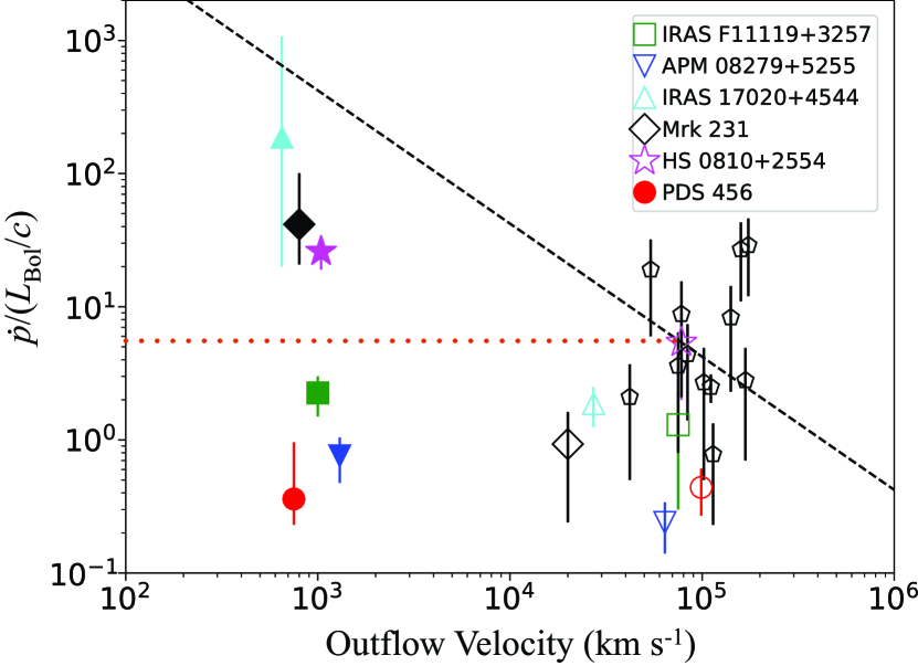
Figure 11: The momentum boost $\dot{{p}}/(L_{Bol}/c)$ as a function of outflow velocity. The filled and unfilled symbols correspond to the molecular and ultrafast outflows, respectively. The dashed and dotted lines represent the dependence of the momentum boost with outflow velocity for energy-conserving and momentum-conserving outflows, respectively for HS 0810+2554. The data from this work are the open pentagon symbols. The data for AGN other than this work have been obtained from the literature (Bischetti et al., 2019; Tombesi et al., 2015; Veilleux et al., 2017; Feruglio et al., 2017, 2015; Chartas et al., 2020).

An indicator of the impact of an ultrafast outflow on the interstellar medium is the momentum boost, $\dot{{p}}_{\rm mo}/(L_{Bol}/c)$. In Figure 11 we show the momentum boost plotted against the outflow velocity for the ultrafast outflows of the high-z quasars presented in this work. For comparison, we also show the momentum boosts and velocities of the ultrafast and molecular outflows of several other AGNs based on published results (see Chartas et al., 2020, and references therein). Half of our sample of high-$z$ quasars have momentum boosts that are considerably larger than those presently known to have both ultrafast and molecular outflows. If the small-scale relativistic outflows drive large-scale molecular outflows we predict that a large fraction of the quasars in our sample will also show molecular outflows with considerably larger momentum boosts than the comparison AGN sample shown in Figure 11. We note, however, that this prediction assumes that the energetics of the ultrafast winds have not varied significantly over the past $10^{6}-10^{7}$ years, the time for the impact of these winds to travel to the observed distances ($1-10$ kpc) of molecular outflows.

6 Conclusions

We presented results from a comprehensive study of UFOs detected in a heterogeneous sample of fourteen quasars in a redshift range of 1.41 – 3.91. A unique and unifying characteristic of our quasar sample is that all the X-ray observations display high quality spectra, to our knowledge, the best for quasars with $z\lower 2.0pt\hbox{$\,\buildrel\scriptstyle>\over{\scriptstyle\sim}\,$}1$. Seven of these 14 quasars have reported ultrafast outflows in the literature, and one, SDSS J1029$+$2623, was previously studied but not searched for UFOs. Six of the 14 quasars of our sample, referred to as our subsample, were selected to contain a UV NAL without prior knowledge of the existence of a UFO. This subsample is therefore unbiased towards UFO detection and is used to infer the fraction of $z>1$ NAL quasars that contain UFOs.

The main conclusions of our spectral analyses of a sample of 14 high-$z$ quasars are the following:

1. Ultrafast outflows of X-ray absorbing material are a common property of our sample of 14 high-$z$ quasars (1.44 $<z<$3.91). Interestingly, all objects but one show UFO signatures. We have detected a UFO in the lensed quasar SDSS J1029+2623, that was previously studied but not searched for UFOs. Our current study has almost doubled the number of detected UFOs in quasars at $z>1.4$. The presence of ultrafast outflows is also supported by the detection of P-Cygni profiles in a large fraction of the sample. Specifically, we find that the X-ray spectra of 5(3) of the 14(6) quasars in our sample(subsample) contain P-Cygni profiles.

2. The estimated momentum boosts of 12 of the 14 quasars in our sample are $\dot{p}/(L_{\rm Bol}/c)$ $>$ 1. Numerical calculations (e.g., Hopkins et al., 2016; Gaspari et al., 2020) have demonstrated that high-velocity winds with momentum fluxes of $\sim L/c$ suppress the star formation rate and black hole accretion rate in the galactic nucleus. The estimated momentum boosts for our sample confirm that relativistic winds of high-$z$ quasars have a dramatic effect on the circum-BH ISM.

3. Relativistic outflows are detected (at $>$ 99% confidence) in 5 of the 6 lensed quasars of our subsample of quasars that were selected to contain a UV NAL. Based on our estimated coverage fractions and UV outflow velocities, all the quasars of our subsample contain outflows of UV absorbing gas with velocities ranging between 5,160 km s^-1 and 22,740 km s^-1. The coexistence of UV NALs and ultrafast outflows is found to be significant in $>$ 83% of the six quasars selected to contain a UV NAL. For comparison, the fraction of AGN that contain ultrafast outflows in samples that are unbiased with respect to the presence of UV winds is about 40% (Tombesi et al., 2010; Gofford et al., 2013). Despite the variable AGN feedback duty cycle involved and the small subsample size, our findings suggest a key link between multiphase AGN feedback properties of the micro-scale UFOs and meso-scale UV outflows, as predicted by theoretical models (e.g., Gaspari et al., 2020).

4. We find a possible anti-correlation between the maximum velocities of the outflowing UV and X-ray absorbers of the NAL quasars in our sample. This anti-correlation also supports a possible link between the micro-scale UFOs and meso-scale UV outflows. An increase of the number of high-$z$ NAL quasars by at least a factor of two will be required to confirm this anti-correlation.

5. The large kinematic luminosities of the ultrafast outflows compared to their bolometric luminosities (see Figures 5 and 6) implies that radiation driving alone cannot explain the acceleration of these winds. We propose that magnetic driving may be a significant contributor to their acceleration as predicted by numerical simulations (Sadowski & Gaspari, 2017).

6. Our high-$z$ quasar sample has outflow velocities ranging between $\sim$ 0.1 and $\sim$ 0.6$c$, significantly higher than those found in low-redshift AGN (see Figure 8). We find no significant dependence between outflow velocities and bolometric luminosity for the high-$z$ quasar sample suggesting that an additional driving mechanism may be contributing to the outflow and/or that relativistic beaming is producing a saturation effect in the acceleration process for velocities $\,\buildrel\scriptstyle>\over{\scriptstyle\sim}\,$ 0.1$c$. For the combined fit to the Tombesi and Gofford samples of low-$z$ AGN and our high-$z$ quasar sample we find a best-fit value of the power-law exponent of $b=0.20\pm 0.03$. This power-law exponent is significantly below the predicted value of $\sim$ 0.5 for radiation driving suggesting that another driving mechanism, such as magnetic driving, may be contributing to the acceleration of the outflow. This possibility is also suggested by the extreme kinetic luminosities and power boosts of a large fraction of the quasars in our sample.

CXO, XMM-Newton, SDSS

Table 1: Properties of Quasar Sample

Object	Classification	$z_{\rm s}$	$z_{\rm l}$	$N^{Gal}_{\rm H}$	$\log(M_{\rm BH})$
				($10^{20}~{}{\rm cm}^{-2}$)	(M⊙)
APM 08279+5255	BALQSO	3.91	1.01	3.84	10.0${}^{+0.1}_{-0.1}$c
HS 1700+6416	NALQSO	2.735	–	2.66	10.2${}^{+0.2}_{-0.2}$d
MG J0414+0534	QSO	2.64	0.9584	11.4	9.0${}^{+0.2}_{-0.2}$e
SDSS J1442+4055	NALQSO	2.593	$\sim$0.4	1.30	$9.7^{+0.2}_{-0.2}$d
SDSS J1029+2623	NALQSO	2.197	0.58	1.78	8.8${}^{+0.2}_{-0.2}$d
SDSS J1529+1038	NALQSO	1.984	$\sim$0.4	2.72	8.9${}^{+0.2}_{-0.2}$d
SDSS J0904+1512	NALQSO	1.826	$\sim$0.3	3.69	9.3${}^{+0.2}_{-0.2}$d
PG 1115+080	mini-BALQSO	1.72	0.31	3.53	8.8${}^{+0.2}_{-0.2}$f
Q 2237+0305	QSO	1.695	0.0386	5.43	9.1${}^{+0.4}_{-0.4}$f
SDSS J1353+1138	NALQSO	1.627	$\sim$0.25	1.86	9.4${}^{+0.2}_{-0.2}$d
SDSS J1128+2402	NALQSO	1.608	–h	1.15	8.7${}^{+0.2}_{-0.2}$d
PID352	QSO	$\sim$1.6	–	0.70	8.7${}^{+0.4}_{-0.4}$g
HS 0810+2554	NALQSO	1.51	0.08	3.94	8.6${}^{+0.2}_{-0.2}$f
SDSS J0921+2854	NALQSO	1.41	0.445	2.30	8.9${}^{+0.2}_{-0.2}$d

Table 2: Log of Observations of Chandra and XMM-Newton  Quasar Sample

				Effective
Object	Observation	Observatory	Observational	Exposure Time	$N_{sc}$
	Date		ID	(ks)	(counts)
APM 08279+5255	2002 Feb 24	Chandra	2979	88.8	5,636$\pm$75
APM 08279+5255	2002 April 28	XMM-Newton	0092800201	83.46/72.59/73.32	13,053$\pm$140/3,307$\pm$59/3,283$\pm$59
APM 08279+5255	2007 Oct 6	XMM-Newton	0502220201	56.38/59.85/43.74	11,400$\pm$114/3,547$\pm$62/2,418$\pm$51
APM 08279+5255	2007 Oct 22	XMM-Newton	0502220301	60.37/72.70/72.14	16,698$\pm$133/5,847$\pm$78/5,589$\pm$77
APM 08279+5255	2008 Jan 14	Chandra	7684	88.1	6,938$\pm$83
HS 1700+6416	2000 Oct 31	Chandra	547	49.5	380$\pm$20
MG J0414+0534	2017 Mar 11	XMM-Newton	0781210301	59.4/71.52/71.55	5,319$\pm$77/1,814$\pm$44/1,991$\pm$46
SDSS J1442+4055	2019 Jan 18	XMM-Newton	0822530101	51.2/ 86.2/85.4	2,190$\pm$48 / 720$\pm$29 / 920 $\pm$ 32
SDSS J1029+2623	2010 Mar 11	Chandra	11755	111.5	2,280$\pm$48
SDSS J1529+1038	2015 July 19	XMM-Newton	0762520201	80.3/91.1/91.3	1,826$\pm$45/460$\pm$22/499$\pm$23
SDSS J0904+1512	2015 Nov 8	XMM-Newton	0762520101	49.8/72.9/74.7	1,493$\pm$41/677$\pm$27/795$\pm$30
PG 1115+080	2001 Nov 25	XMM-Newton	0082340101	52.37/60.40/60.04	10,783$\pm$109/3,369$\pm$60/3,299$\pm$60
PG 1115+080	2004 Jun 10	XMM-Newton	0203560201	51.47/66.07/66.13	10,814$\pm$107/3,855$\pm$64/3,544$\pm$61
PG 1115+080	2004 Jun 26	XMM-Newton	0203560401	54.92/81.88/81.88	9,867$\pm$105/4,247$\mp$65/3,943$\pm$65
Q 2237+0305	2017 Jan 4	Chandra	19639	32.92	577$\pm$24
SDSS J1353+1138	2016 Jan 13	XMM-Newton	0762520101	31.80/51.08/50.29	1,788$\pm$44/748$\pm$29/845$\pm$31
SDSS J1128+2402	2018 May 28	XMM-Newton	0822530201	29.27/35.12/35.14	1,994$\pm$47/409$\pm$22/547$\pm$ 25
PID352	c	XMM-Newton	c	3450	2,560/690/1,250
HS 0810+2554	2013 Dec 16	Chandra	16110	97.73	5,776$\pm$76
HS 0810+2554	2016 Dec 23	Chandra	18204	96.76	8,525$\pm$92
HS 0810+2554	2014 Oct 04	XMM-Newton	0728990101	46.4/54.97/54.99	11,811$\pm$114/3,131$\pm$59/3,009$\pm$56
SDSS J0921+2854	2018 May 15	XMM-Newton	0822530301	/32.75/32.76	/2,425$\pm$50/2,625$\pm$52
SDSS J0921+2854	2018 Oct 24	XMM-Newton	0822530501	25.34/30.69/30.73	9,991$\pm$105/2,885$\pm$55/2,978$\pm$55

Table 3: Luminosities of Quasar Sample

Object	Observation	$f_{\rm 2-10~{}keV}$	$L_{\rm 2-10~{}keV}$	$L_{\rm ion}$	$\log({\lambda}L_{\lambda}/\rm erg~{}s^{-1})$d	$\log(L_{\rm Bol}/\rm erg~{}s^{-1})$	$L_{\rm Bol}/L_{\rm Edd}$	$\mu$
	Date	(erg s-1)	(erg s-1)	(erg s-1)	$1450~{}{\rm\AA}$	2$-$10 keV/$1450~{}{\rm\AA}$
APM 08279+5255	2002 Feb 24	4.3${}^{+0.2}_{-0.1}$	$43^{+2}_{-1}$	$12^{+0.6}_{-0.3}$	–	47.9/47.83g	0.57${}_{-0.13}^{+0.16}$	4
APM 08279+5255	2002 April 28	4.1${}^{+0.2}_{-0.2}$	$53^{+3}_{-3}$	$18^{+1.0}_{-1.0}$	–	48.0/47.83g	0.57${}_{-0.16}^{+0.19}$	4
APM 08279+5255	2007 Oct 6	3.9${}^{+0.2}_{-0.2}$	$67^{+3}_{-3}$	$32^{+1.4}_{-1.4}$	–	48.2/47.83g	0.57${}_{-0.26}^{+0.28}$	4
APM 08279+5255	2007 Oct 22	5.0${}^{+0.2}_{-0.2}$	$95^{+3}_{-3}$	$56^{+1.8}_{-1.8}$	–	48.4/47.83g	0.57${}_{-0.35}^{+0.38}$	4
APM 08279+5255	2008 Jan 14	4.5${}^{+0.2}_{-0.2}$	$65^{+3}_{-3}$	$25^{+1.2}_{-1.2}$	–	48.2/47.83g	0.57${}_{-0.26}^{+0.28}$	4
HS 1700+6416	2000 Oct 31	0.55${}^{+0.1}_{-0.05}$	2.3${}^{+0.5}_{-0.2}$	$0.62^{+0.1}_{-0.1}$	47.67	47.0/48.15	0.8${}_{-0.5}^{+1.3}$	1
MG J0414+0534	2017 Mar 11	3.3${}^{+0.02}_{-0.02}$	$15.0^{+0.1}_{-0.2}$	$3.9^{+0.4}_{-0.4}$	–	45.9/46.56h	0.26${}_{-0.15}^{+0.35}$	47
SDSS J1442+4055	2019 Jan 18	2.5${}^{+0.1}_{-0.1}$	$3.7^{+0.2}_{-0.2}$	$1.2^{+0.2}_{-0.2}$	46.10	46.2/46.6	0.06${}_{-0.03}^{+0.06}$	6.3
SDSS J1029+2623	2010 Mar 11	1.7${}^{+0.1}_{-0.1}$	$3.4^{+0.2}_{-0.2}$	$0.68^{+0.04}_{-0.04}$	44.82	45.3/45.40	0.03${}_{-0.01}^{+0.02}$	30
SDSS J1529+1038	2015 July 19	0.31${}^{+0.10}_{-0.10}$	$0.8^{+0.3}_{-0.3}$	$0.21^{+0.08}_{-0.08}$	45.54	45.33/46.06	0.12${}_{-0.07}^{+0.14}$	7
SDSS J0904+1512	2015 Nov 8	0.75${}^{+0.1}_{-0.1}$	$1.6^{+0.3}_{-0.3}$	$0.66^{+0.09}_{-0.09}$	45.62	45.6/46.13	0.06${}_{-0.03}^{+0.06}$	9
PG 1115+080	2001 Nov 25	4.0${}^{+0.1}_{-0.1}$	$6.6^{+0.2}_{-0.2}$	$1.94^{+0.06}_{-0.06}$	45.47	45.4/46.0	0.16${}_{-0.09}^{+0.18}$	46
PG 1115+080	2004 Jun 26	4.0${}^{+0.1}_{-0.1}$	$7.6^{+0.2}_{-0.2}$	$2.76^{+0.07}_{-0.07}$	45.47	45.5/46.0	0.16${}_{-0.09}^{+0.18}$	46
PG 1115+080	2004 Jun 10	3.5${}^{+0.2}_{-0.2}$	$6.3^{+0.3}_{-0.3}$	$2.14^{+0.09}_{-0.09}$	45.47	45.4/46.0	0.16${}_{-0.09}^{+0.18}$	46
Q 2237+0305	2017 Jan 4	1.9${}^{+0.1}_{-0.1}$	$2.2^{+0.1}_{-0.1}$	$0.43^{+0.02}_{-0.02}$	45.53	45.4/46.05	0.08${}_{-0.04}^{+0.10}$	16
SDSS J1353+1138	2016 Jan 13	1.2${}^{+0.2}_{-0.2}$	$2.1^{+0.3}_{-0.3}$	$0.8^{+0.1}_{-0.1}$	46.32	46.1/46.75	0.20${}_{-0.11}^{+0.22}$	4
SDSS J1128+2402	2018 May 28	1.1${}^{+0.3}_{-0.2}$	$1.3^{+0.4}_{-0.3}$	$0.23^{+0.03}_{-0.03}$	45.46	45.7/46.0	0.15${}_{-0.07}^{+0.13}$	6
PID352		0.28${}^{+0.03}_{-0.03}$	2.8${}^{+0.3}_{-0.3}$	–	–	45.9/$46.0$	0.13${}_{-0.07}^{+0.17}$	1
HS 0810+2554	2013 Dec 16	3.3${}^{+0.1}_{-0.2}$	$4.8^{+0.4}_{-0.4}$	$1.9^{+0.2}_{-0.2}$	45.04	44.9/45.6	0.08${}_{-0.04}^{+0.10}$	103
HS 0810+2554	2016 Dec 23	5.2${}^{+0.5}_{-0.5}$	$7.8^{+0.8}_{-0.8}$	$3.0^{+0.3}_{-0.3}$	45.04	45.1/45.6	0.08${}_{-0.04}^{+0.10}$	103
HS 0810+2554	2014 Oct 04	3.1${}^{+0.1}_{-0.1}$	$4.6^{+0.4}_{-0.4}$	$3.6^{+0.3}_{-0.3}$	45.04	44.9/45.6	0.08${}_{-0.04}^{+0.10}$	103
SDSS J0921+2854	2018 May 15	6.8${}^{+0.2}_{-0.2}$	$6.2^{+0.2}_{-0.2}$	$1.6^{+0.2}_{-0.2}$	44.80	46.7/45.4	0.03${}_{-0.02}^{+0.04}$	4
SDSS J0921+2854	2018 Oct 24	6.9${}^{+0.2}_{-0.2}$	$7.3^{+0.2}_{-0.2}$	$1.3^{+0.2}_{-0.2}$	44.80	46.8/45.4	0.03${}_{-0.02}^{+0.04}$	4

Table 4: Results from Fits to the Spectra of SDSS J1442+4055, SDSS J1029+2623, and SDSS J1529+1038.

Modela	Parameterb	Fitted Valuesc	Fitted Valuesc	Fitted Valuesc
		SDSS J1442	SDSS J1029	SDSS J1529
${1}$	$\Gamma$	1.80${}_{-0.12}^{+0.12}$	1.54${}_{-0.06}^{+0.06}$	2.0${}_{-0.1}^{+0.1}$
	$N_{\rm H}$	—	$<$ 0.4 $\times$1022 cm-2	—
	$\chi^{2}/{\nu}$	55.07/58	60.1/82	33.3/39
	$P(\chi^{2}/{\nu})$d	5.8 $\times$ 10-1	9.7 $\times$ 10-1	7.3 $\times$ 10-1
${2}$	$\Gamma$	1.80${}_{-0.14}^{+0.08}$	1.49${}_{-0.06}^{+0.06}$	1.85${}_{-0.15}^{+0.19}$
	$N_{\rm H}$	—	$<$ 0.4 $\times$1022 cm-2	—
	E1	9.14${}_{-0.2}^{+0.2}$ keV	13.3${}_{-0.9}^{+0.7}$ keV	9.0${}_{-1.5}^{+1.5}$ keV
	$\sigma_{\rm 1}$	$<$ 0.1 keV	0.7${}_{-0.7}^{+1.2}$ keV	$<$ 2.8 keV
	EW1	$-$194${}_{-160}^{+150}$ eV	$-$610${}_{-245}^{+240}$ eV	$-$1.8${}_{-348}^{+404}$ keV
	E2	11.3${}_{-0.6}^{+0.6}$ keV	—	—
	$\sigma_{\rm 2}$	$<$ 0.2 keV	—	—
	EW2	$-$546${}_{-200}^{+220}$ eV	—	—
	E3	16.44${}_{-0.2}^{+0.2}$ keV	—	—
	$\sigma_{\rm 3}$	$<$ 0.1 keV	—	—
	EW3	$+$1.3${}_{-0.5}^{+0.6}$ keV	—	—
	$\chi^{2}/{\nu}$	45.00/54	53.8/80	26.8/36
	$P(\chi^{2}/{\nu})$d	8.03 $\times$ 10-1	9.9 $\times$ 10-1	8.7 $\times$ 10-1
	$F_{1}/F_{2}/F_{3}{}^{e}$	7.1/7.4/13.8	5.08/–/–	5.13/–/–
	$P_{\rm MC,1}/P_{\rm MC,2}/P_{\rm MC,3}{}^{f}$	1.2$\times$10-2/8.0$\times$10-3/1.0$\times$10-3	6.7$\times$10-3/–/–	1$\times$10-2/–/–
${3}$	$\Gamma$	1.79${}_{-0.14}^{+0.14}$	1.47${}_{-0.06}^{+0.07}$	1.90${}_{-0.07}^{+0.07}$
	$N_{\rm H}$	—	$<$ 0.4$\times$1022 cm-2	—
	E1	16.35${}_{-0.2}^{+0.2}$ keV	—	—
	$\sigma_{\rm 1}$	$<$ 0.1 keV	—	—
	EW1	$+$1.5${}_{-0.1}^{+0.1}$ keV	—	—
	$N_{\rm Habs1}$	3.5${}_{-1.7}^{+1.5}$ $\times$ 1023 cm-2(68%)	7.4${}_{-2.4}^{+2.6}$ $\times$ 1023 cm-2(68%)	3.2${}_{-2}^{+5}$ $\times$ 1023 cm-2(68%)
	$\log\xi_{\rm abs1}$	3.2${}_{-0.1}^{+0.1}$ erg cm s-1(68%)	2.8${}_{-0.1}^{+0.1}$ erg cm s-1(68%)	3.6${}_{-0.4}^{+0.4}$ erg cm s-1(68%)
	$v_{\rm turb,abs1}$	15,000 km s-1	19,000 km s-1	36,000 km s-1
	$z_{\rm abs1}$	1.16${}_{-0.10}^{+0.12}$	0.66${}_{-0.04}^{+0.05}$	1.31${}_{-0.2}^{+0.2}$
	$\chi^{2}/{\nu}$	36.79/56	55.13/79	26.7/37
	$P(\chi^{2}/{\nu})$d	9.7 $\times$ 10-1	9.8 $\times$ 10-1	9.0 $\times$ 10-1

Table 5: Results from Fits to the Spectra of SDSS J1353+1138, SDSS J0904+1512, and Q 2237+0305.

Modela	Parameterb	Fitted Valuesc	Fitted Valuesc	Fitted Valuesc
		SDSS J1353	SDSS J0904	Q 2237
${1}$	$\Gamma$	2.16${}_{-0.12}^{+0.15}$	2.02${}_{-0.14}^{+0.15}$	1.76 ${}_{-0.24}^{+0.26}$
	$N_{\rm H}$	0.61 ${}_{-0.26}^{+0.30}$$\times$1022 cm-2	0.25 ${}_{-0.25}^{+0.36}$$\times$1022 cm-2	1.42${}_{-1.34}^{+1.55}$$\times$1022 cm-2
	$\chi^{2}/{\nu}$	61.14/76	49.6/75	42.16/33
	$P(\chi^{2}/{\nu})$d	8.9 $\times$ 10-1	9.9 $\times$ 10-1	1.3 $\times$ 10-1
${2}$	$\Gamma$	2.12${}_{-0.19}^{+0.16}$	1.96${}_{-0.13}^{+0.16}$	1.64 ${}_{-0.24}^{+0.26}$
	$N_{\rm H}$	0.56 ${}_{-0.27}^{+0.30}$$\times$1022 cm-2	0.16 ${}_{-0.16}^{+0.36}$$\times$1022 cm-2	1.51${}_{-1.21}^{+1.50}$$\times$1022 cm-2
	E1	8.6${}_{-0.3}^{+0.2}$ keV	9.0${}_{-1.6}^{+0.7}$ keV	6.58${}_{-0.09}^{+0.14}$ keV
	$\sigma_{\rm 1}$	0.33${}_{-0.33}^{+0.45}$ keV	$<$ 1.5 keV	$<$ 0.2 keV
	EW1	$+$1.6${}_{-1.1}^{+1.1}$ keV	$-$650${}_{-230}^{+290}$ eV	+805${}_{-230}^{+260}$ eV
	E2	9.3${}_{-0.6}^{+0.6}$ keV	—	7.3${}_{-1.2}^{+1.2}$ keV
	$\sigma_{\rm 2}$	0.78 ${}_{-0.78}^{+1.4}$ keV	—	1.9 ${}_{-0.9}^{+1.7}$ keV
	EW2	$-$947${}_{-375}^{+462}$ eV	—	$-$1620${}_{-460}^{+810}$ eV
	E3	—	—	—
	$\sigma_{\rm 3}$	—	—	—
	EW3	—	—	—
	$\chi^{2}/{\nu}$	52.02/71	43.8/72	25.61 /27
	$P(\chi^{2}/{\nu})$d	9.56 $\times$ 10-1	9.96 $\times$ 10-1	5.4 $\times$ 10-1
	$F_{1}/F_{2}/F_{3}{}^{e}$	13.6/13.8/–	4.80/–/–	12.5 /12.5 /–
	$P_{\rm MC,1}/P_{\rm MC,2}/P_{\rm MC,3}{}^{f}$	3.0$\times$10-3/1.0$\times$10-2/–	3.5$\times$10-2/–/–	4$\times$10-3/2$\times$10-3/–
${3}$	$\Gamma$	2.10${}_{-0.12}^{+0.11}$	1.97${}_{-0.13}^{+0.14}$	1.59${}_{-0.22}^{+0.25}$
	$N_{\rm H}$	0.56 ${}_{-0.25}^{+0.30}$$\times$1022 cm-2	0.15${}_{-0.15}^{+0.15}$$\times$1022 cm-2	0.94 ${}_{-0.94}^{+0.14}$$\times$1022 cm-2
	E1	8.5${}_{-0.6}^{+0.5}$ keV	—	6.59${}_{-0.09}^{+0.14}$ keV
	$\sigma_{\rm 1}$	$<$ 0.1 keV	—	$<$ 0.2 keV
	EW1	$+$460${}_{-380}^{+430}$ eV	—	+480${}_{-180}^{+190}$ eV
	$N_{\rm Habs1}$	3.9${}_{-2.3}^{+2.4}$ $\times$ 1023 cm-2(68%)	3.3${}_{-2.0}^{+3.0}$ $\times$ 1023 cm-2(68%)	1.0${}_{-0.4}^{+0.4}$ $\times$ 1024 cm-2
	$\log\xi_{\rm abs1}$	3.6${}_{-0.1}^{+0.2}$ erg cm s-1(68%)	3.6${}_{-0.1}^{+0.4}$ erg cm s-1(68%)	3.10${}_{-0.3}^{+0.2}$ erg cm s-1(68%)
	$v_{\rm turb,abs1}$	10,000 km s-1	11,000 km s-1	30,000 km s-1
	$z_{\rm abs1}$	0.85${}_{-0.05}^{+0.20}$	1.15${}_{-0.12}^{+0.10}$	1.27${}_{-0.12}^{+0.18}$
	$\chi^{2}/{\nu}$	56.5/73	45.4/71	28.6/29
	$P(\chi^{2}/{\nu})$d	9.24 $\times$ 10-1	9.92 $\times$ 10-1	4.9 $\times$ 10-1

Table 6: Results from Fits to the X-ray Spectra of SDSS J1128+2402 and SDSS J0921+2854

Modela	Parameterb	Fitted Valuesc	Fitted Valuesc	Fitted Valuesc
		SDSS J1128	SDSS J0921 (OBS1)	SDSS J0921 (OBS2)
${1}$	$\Gamma$	1.92${}_{-0.08}^{+0.09}$	1.69${}_{-0.07}^{+0.08}$	1.72${}_{-0.13}^{+0.13}$
	$N_{\rm H}$	—	—	—
	$\chi^{2}/{\nu}$	68.53/85	81.9/79	68.21/88
	$P(\chi^{2}/{\nu})$d	9.03 $\times$ 10-1	4.10 $\times$ 10-1	9.42 $\times$ 10-1
${2}$	$\Gamma$	1.88${}_{-0.09}^{+0.1}$	1.63${}_{-0.08}^{+0.08}$	1.68${}_{-0.13}^{+0.13}$
	$N_{\rm H}$	—	—	—
	E1	11.7${}_{-0.19}^{+0.15}$ keV	10.3${}_{-0.05}^{+0.08}$ keV	10.45${}_{-0.21}^{+0.31}$ keV
	$\sigma_{\rm 1}$	$<$ 1 keV	$<$ 0.1 keV	$<$ 0.1 keV
	EW1	$+$2.3${}_{-0.5}^{+0.3}$ keV	$+$0.75${}_{-0.31}^{+0.39}$ keV	$+$143${}_{-50}^{+60}$ eV
	E2	12.4${}_{-1.1}^{+1.2}$ keV	10.45${}_{-0.42}^{+0.29}$ keV	12.56${}_{-0.16}^{+0.13}$ keV
	$\sigma_{\rm 2}$	$+$1.1${}_{-0.5}^{+1.2}$ keV	$+$0.52${}_{-0.47}^{+0.52}$ keV	$<$ 0.1 keV
	EW2	$-$880${}_{-1280}^{+80}$ eV	$-$0.45${}_{-0.19}^{+0.12}$ keV	$-$217${}_{-120}^{+10}$ eV
	E3	—	—	6.39${}_{-0.99}^{+0.86}$ keV
	$\sigma_{\rm 3}$	—	—	$<$ 0.1 keV
	EW3	—	—	$+$100${}_{-60}^{+55}$ eV
	$\chi^{2}/{\nu}$	61.52/84	64.11/73	54.54/82
	$P(\chi^{2}/{\nu})$d	9.69 $\times$ 10-1	7.62 $\times$ 10-1	9.92 $\times$ 10-1
	$F_{1}/F_{2}/F_{3}{}^{e}$	10.4/11.3/–	11.7/11.8/–	10.8/8.4/8.2
	$P_{\rm MC,1}/P_{\rm MC,2}/P_{\rm MC,3}{}^{f}$	5.3$\times$10-3/8.0$\times$10-3/–	8.0$\times$10-3/9.0$\times$10-3/–	1.5$\times$10-3/ 6.0$\times$10-3/9.3$\times$10-3
${3}$	$\Gamma$	1.88${}_{-0.04}^{+0.04}$	1.58${}_{-0.14}^{+0.14}$	1.63${}_{-0.08}^{+0.09}$
	$N_{\rm H}$	—	—	—
	E1	11.4${}_{-0.2}^{+0.1}$ keV	10.3${}_{-0.11}^{+0.09}$ keV	10.4${}_{-0.18}^{+0.21}$ keV
	$\sigma_{\rm 1}$	$<$ 0.1 keV	$<$ 0.1 keV	$<$ 0.1 keV
	EW1	$+$1.2${}_{-0.8}^{+0.9}$ keV	$+$315${}_{-265}^{+280}$ eV	$+$124${}_{-120}^{+100}$ eV
	$N_{\rm Habs1}$	2.3${}_{-1.7}^{+1.3}$ $\times$ 1023 cm-2(68%)	3.7${}_{-1.5}^{+2.4}$ $\times$ 1023 cm-2(68%)	6${}_{-3}^{+3}$ $\times$ 1023 cm-2(68%)
	$\log\xi_{\rm abs1}$	3.15${}_{-0.15}^{+0.15}$ erg cm s-1(68%)	3.1${}_{-0.3}^{+0.2}$ erg cm s-1(68%)	3.14${}_{-0.04}^{+0.1}$ erg cm s-1(68%)
	$v_{\rm turb,abs1}$	9,000 km s-1	3,000 km s-1	6,000 km s-1
	$z_{\rm abs1}$	0.39${}_{-0.03}^{+0.03}$	0.56${}_{-0.02}^{+0.03}$	0.33${}_{-0.02}^{+0.02}$
	$\chi^{2}/{\nu}$	30.42/46	65.15/72	86.63/120
	$P(\chi^{2}/{\nu})$d	9.63 $\times$ 10-1	7.03 $\times$ 10-1	9.90 $\times$ 10-1

Table 7: Results from Fits to the SDSS Spectra of the Subsample

Object	Plate-MJD-Fibera	Compb	$\lambda_{\rm CIV,B}$c	FWHMCIV,B	$\lambda_{\rm CIV,R}$c	FWHMCIV,R	$v_{\rm UV}$
			(Å)	(km s-1)	(Å)	(km s-1)	$(c)$
SDSS J1442+4055	6061-56076-0132	1	1482.68$\pm$0.09	227$\pm$45	1484.89$\pm$0.26	322$\pm$159	0.0423$\pm$0.0001
SDSS J1529+1038	5493-56009-0900	1	1509.79$\pm$0.17	188$\pm$62	1512.33$\pm$0.17	188$\pm$62	0.0248$\pm$0.0001
SDSS J1529+1038	5493-56009-0900	2	1511.06$\pm$0.17	203$\pm$63	1513.78$\pm$0.17	203$\pm$63	0.0239$\pm$0.0001
SDSS J1529+1038	5493-56009-0900	3	1538.32$\pm$0.03	192$\pm$15	1540.95$\pm$0.04	201$\pm$22	0.0063$\pm$0.0001
SDSS J0904+1512	5295-55978-0976	1	1430.86$\pm$0.07	244$\pm$37	1433.17$\pm$0.12	289$\pm$61	0.0758$\pm$0.0001
SDSS J0904+1512	5295-55978-0976	2	1452.87$\pm$0.06	244$\pm$29	1455.04$\pm$0.06	306$\pm$29	0.0616$\pm$0.0001
SDSS J0904+1512	5295-55978-0976	3	1516.10$\pm$0.10	269$\pm$51	1518.47$\pm$0.10	280$\pm$51	0.0207$\pm$0.0001
SDSS J1353+1138	1702-53144-0397	1	1513.26$\pm$0.04	284$\pm$18	1515.92$\pm$0.06	310$\pm$25	0.0226$\pm$0.0001
SDSS J1128+2402	2497-54154-0113	1	1515.71$\pm$0.15	230$\pm$73	1518.14$\pm$0.11	203$\pm$50	0.0210$\pm$0.0001
SDSS J0921+2854	2353-53794-0139	1	1521.55$\pm$0.20	139$\pm$87	1523.69$\pm$0.18	125$\pm$77	0.0172$\pm$0.0001

Table 8: Properties of Outflowing C IV Absorbers of the Subsample

Object	Plate-MJD-Fiber	Comp	$W_{\rm CIV,B}$a	$W_{\rm CIV,R}$a	$C_{\rm f}$b	$\tau$c	$N_{\rm CIV}$d
			(Å)	(Å)			($\times~{}10^{14}$ cm${}^{-2})$
SDSS J1442+4055	6061-56076-0132	1	0.46$\pm$0.10	0.23$\pm$0.10	–	–	–
SDSS J1529+1038	5493-56009-0900	1	0.4$\pm$0.1	0.4$\pm$0.1	–	–	–
SDSS J1529+1038	5493-56009-0900	2	0.5$\pm$0.1	0.5$\pm$0.1	0.21$\pm$0.06	4$\pm$3	3$\pm$2
SDSS J1529+1038	5493-56009-0900	3	1.07$\pm$0.08	0.83$\pm$0.14	0.36$\pm$0.03	1.20$\pm$0.40	1.3$\pm$0.3
SDSS J0904+1512	5295-55978-0976	1	1.5$\pm$0.2	1.2$\pm$0.3	0.85$\pm$0.12	0.36$\pm$0.05	1.3$\pm$0.1
SDSS J0904+1512	5295-55978-0976	2	1.0$\pm$0.2	1.2$\pm$0.4	–	–	–
SDSS J0904+1512	5295-55978-0976	3	0.7$\pm$0.2	0.7$\pm$0.2	0.18$\pm$0.02	3.0$\pm$0.3	2.3$\pm$0.4
SDSS J1353+1138	1702-53144-0397	1	1.80$\pm$0.23	1.70$\pm$0.29	0.51$\pm$0.03	1.4$\pm$0.4	3.2$\pm$0.1
SDSS J1128+2402	2497-54154-0113	1	1.27$\pm$0.30	1.14$\pm$0.30	0.40$\pm$0.04	2.2$\pm$0.5	2.9$\pm$0.2
SDSS J0921+2854	2353-53794-0139	1	0.93$\pm$0.04	0.96$\pm$0.03	–	–	–

Table 9: Quasar Outflow Properties

Object	Observation	$N_{\rm H}$a	$C_{\rm SR}$	$r_{\rm min}$a	$r_{\rm max}/r_{\rm min}$	$\log\xi$a	$v_{\rm wind}$	$\dot{M}$	$\dot{E}$${}_{\rm K}/L_{\rm Bol}$	$\dot{p}/(L_{\rm Bol}/c)$
	Date						($c$)	(M${}_{\odot}~{}{\rm yr}^{-1}$)
APM 08279+5255	2002 Feb 24	10${}^{+6.0}_{-6.0}$	1.44	121${}^{+43}_{-38}$	24	$4.0^{+0.8}_{-0.1}$	$0.16^{+0.02}_{-0.02}$	$101^{+59}_{-53}$	$0.11^{+0.07}_{-0.06}$	$1.35^{+0.84}_{-0.72}$
APM 08279+5255	2002 Feb 24	1.0${}^{+0.8}_{-0.5}$	2.21	25${}^{+7}_{-7}$	7,756	$3.2^{+0.2}_{-0.3}$	$0.35^{+0.03}_{-0.03}$	$5.0^{+3.2}_{-2.6}$	$0.026^{+0.018}_{-0.014}$	$0.15^{+0.10}_{-0.08}$
APM 08279+5255	2002 April 28	1.7${}^{+0.2}_{-0.2}$	1.59	76${}^{+24}_{-22}$	2,926	$3.1^{+0.1}_{-0.7}$	$0.20^{+0.02}_{-0.02}$	$12.7^{+3.9}_{-3.6}$	$0.022^{+0.009}_{-0.007}$	$0.22^{+0.08}_{-0.07}$
APM 08279+5255	2002 April 28	1.4${}^{+0.4}_{-0.8}$	2.77	14${}^{+4}_{-4}$	7,208	$3.5^{+0.8}_{-0.4}$	$0.46^{+0.03}_{-0.03}$	$4.6^{+2.3}_{-2.1}$	$0.04^{+0.02}_{-0.02}$	$0.19^{+0.10}_{-0.09}$
APM 08279+5255	2007 Oct 6	3.9${}^{+1.1}_{-0.9}$	1.51	94${}^{+32}_{-28}$	557	$3.6^{+0.9}_{-0.3}$	$0.18^{+0.02}_{-0.02}$	$33^{+13}_{-11}$	$0.043^{+0.017}_{-0.016}$	$0.61^{+0.42}_{-0.30}$
APM 08279+5255	2007 Oct 6	8.3${}^{+1.0}_{-1.0}$	3.39	10${}^{+3}_{-3}$	1,190	$3.9^{+0.2}_{-0.3}$	$0.54^{+0.03}_{-0.03}$	$23^{+7}_{-6}$	$0.28^{+0.08}_{-0.08}$	$1.3^{+0.9}_{-0.6}$
APM 08279+5255	2007 Oct 22	1.2${}^{+0.2}_{-0.3}$	1.33	178${}^{+51}_{-47}$	5,477	$3.1^{+0.1}_{-0.2}$	$0.13^{+0.02}_{-0.02}$	$14^{+4}_{-4}$	$0.013^{+0.011}_{-0.007}$	$0.20^{+0.17}_{-0.11}$
APM 08279+5255	2007 Oct 22	1.0${}^{+0.2}_{-0.2}$	2.34	21${}^{+6}_{-6}$	53,891	$3.1^{+0.1}_{-0.1}$	$0.38^{+0.03}_{-0.03}$	$4^{+1}_{-1}$	$0.031^{+0.029}_{-0.017}$	$0.16^{+0.15}_{-0.09}$
APM 08279+5255	2008 Jan 14	0.9${}^{+0.4}_{-0.4}$	1.67	63${}^{+2}_{-2}$	5,815	$3.3^{+0.7}_{-0.6}$	$0.22^{+0.02}_{-0.02}$	$6^{+3}_{-3}$	$0.016^{+0.012}_{-0.009}$	$0.14^{+0.11}_{-0.08}$
APM 08279+5255	2008 Jan 14	4.0${}^{+4.0}_{-3.2}$	3.95	8.5${}^{+2.1}_{-2.1}$	2,317	$3.9^{+0.5}_{-0.5}$	$0.59^{+0.03}_{-0.03}$	$13^{+8}_{-7}$	$0.23^{+0.20}_{-0.14}$	$0.77^{+0.62}_{-0.46}$
HS 1700+6416	2000 Oct 31	5.6${}^{+4.4}_{-0}$	2.34	3.1${}^{+1.7}_{-1.5}$	55	$3.9^{+1.0}_{-0.4}$	$0.38^{+0.05}_{-0.05}$	$33^{+21}_{-18}$	$0.10^{+0.09}_{-0.07}$	$0.54^{+0.41}_{-0.36}$
MG J0414+0534	2017 Mar 11	9.8${}^{+5.7}_{-3.6}$	1.91	4.7${}^{+2.9}_{-2.4}$	206	$3.0^{+0.1}_{-0.1}$	$0.28^{+0.05}_{-0.05}$	$6.2^{+4.2}_{-3.6}$	$0.49^{+0.40}_{-0.32}$	$3.5^{+2.3}_{-2.3}$
SDSS J1442+4055	2019 Jan 18	3.5${}^{+1.5}_{-1.7}$	2.83	6.6${}^{+3.1}_{-2.9}$	1,155	$6.6^{+3.1}_{-2.9}$	$0.47^{+0.03}_{-0.05}$	$5.5^{+3.7}_{-3.2}$	$1.2^{+0.9}_{-0.8}$	$5.1^{+4.0}_{-3.2}$
SDSS J1029+2623	2010 Mar 11	7.4${}^{+2.6}_{-2.4}$	3.82	0.6${}^{+0.2}_{-0.2}$	880	$2.8^{+0.1}_{-0.1}$	$0.58^{+0.01}_{-0.02}$	$0.9^{+0.6}_{-0.5}$	$4.3^{+2.9}_{-2.5}$	$15^{+10}_{-8}$
SDSS J1529+1038	2015 July 19	3.2${}^{+4.9}_{-1.9}$	1.79	5.6${}^{+4.5}_{-3.4}$	62	$3.6^{+0.4}_{-0.4}$	$0.25^{+0.06}_{-0.08}$	$2.0^{+1.6}_{-1.2}$	$0.37^{+0.26}_{-0.26}$	$3.0^{+2.3}_{-2.0}$
SDSS J0904+1512	2015 Nov 8	4.0${}^{+2.3}_{-2.4}$	1.83	9.1${}^{+5.5}_{-4.5}$	59	$3.84^{+0.16}_{-0.19}$	$0.26^{+0.05}_{-0.04}$	$4.8^{+2.6}_{-2.9}$	$0.9^{+0.7}_{-0.6}$	$6.9^{+5.8}_{-4.7}$
PG 1115+080	2001 Nov 25	1.9${}^{+0.5}_{-0.5}$	1.17	23${}^{+12}_{-11}$	63	$3.23^{+0.07}_{-0.03}$	$0.08^{+0.02}_{-0.02}$	$1.7^{+1.0}_{-0.9}$	$0.045^{+0.039}_{-0.028}$	$1.1^{+0.8}_{-0.6}$
PG 1115+080	2001 Nov 25	1.6${}^{+0.4}_{-0.3}$	2.30	1.4${}^{+0.5}_{-0.5}$	1913	$3.14^{+1.2}_{-0.03}$	$0.37^{+0.01}_{-0.01}$	$0.31^{+0.16}_{-0.14}$	$0.17^{+0.12}_{-0.11}$	$0.9^{+0.2}_{-0.1}$
Q 2237+0305	2017 Jan 4	10${}^{+4}_{-4}$	1.51	30${}^{+25}_{-24}$	18	$3.1^{+0.2}_{-0.3}$	$0.18^{+0.06}_{-0.09}$	$16^{+13}_{-10}$	$1.58^{+1.24}_{-1.10}$	$17.5^{+10}_{-11}$
SDSS J1353+1138	2016 Jan 1	3.9${}^{+2.4}_{-2.3}$	2.16	7.3${}^{+4.1}_{-3.4}$	213	$3.6^{+0.2}_{-0.1}$	$0.34^{+0.02}_{-0.09}$	$11.2^{+3.7}_{-3.0}$	$0.18^{+0.24}_{-0.23}$	$2.0^{+1.8}_{-1.4}$
SDSS J1128+2402	2018 May 28	2.3${}^{+1.7}_{-1.3}$	3.60	0.5${}^{+0.2}_{-0.2}$	1,949	$3.15^{+0.15}_{-0.15}$	$0.56^{+0.01}_{-0.02}$	$0.35^{+0.25}_{-0.21}$	$0.41^{+0.34}_{-0.27}$	$1.5^{+1.3}_{-1.0}$
PID352		2.2${}^{+3.1}_{-1.6}$	1.36	12${}^{+9}_{-7}$		$2.9^{+1.47}_{-0.38}$	$0.14^{+0.02}_{-0.06}$	$1.9^{+1.7}_{-1.2}$	$0.14^{+0.11}_{-0.09}$	1.95${}^{+1.65}_{-1.23}$
HS 0810+2554	2014 Oct 04	2.1${}^{+1.0}_{-1.1}$	1.26	11${}^{+7}_{-5}$	1.5	$5.0^{+1.0}_{-0.4}$	$0.11^{+0.05}_{-0.03}$	$1.2^{+0.9}_{-0.7}$	$0.15^{+0.14}_{-0.10}$	$2.6^{+2.2}_{-1.9}$
HS 0810+2554	2014 Oct 04	1.4${}^{+0.3}_{-0.5}$	2.59	0.7${}^{+0.3}_{-0.3}$	317	$4.1^{+0.4}_{-0.2}$	$0.43^{+0.04}_{-0.05}$	$0.21^{+0.12}_{-0.11}$	$0.35^{+0.23}_{-0.22}$	$1.7^{+1.1}_{-1.1}$
SDSS J0921+2854	2018 May 15	3.7${}^{+2.4}_{-1.5}$	2.49	1.3${}^{+0.6}_{-0.6}$	6,381	$3.1^{+0.2}_{-0.3}$	$0.41^{+0.02}_{-0.01}$	$1.1^{+0.8}_{-0.6}$	$2.6^{+2.4}_{-1.9}$	13${}^{+12}_{-9}$
SDSS J0921+2854	2018 Oct 24	6.0${}^{+2.7}_{-2.4}$	3.30	0.8${}^{+0.3}_{-0.3}$	62	$3.14^{+0.1}_{-0.04}$	$0.53^{+0.01}_{-0.01}$	$1.3^{+0.9}_{-0.7}$	$5.2^{+3.9}_{-3.7}$	$20^{+13}_{-14}$

Note. — The properties of the outflowing X-ray absorbing gas are obtained from the photoionization model XSTAR. $\dot{M}$, $\dot{E}$_K, and $\dot{p}$ are derived from equations 1, 2, and 3, respectively. To correct for relativistic effects proposed in Luminary et al. 2020, the values of $N_{\rm H}$, $\dot{M}$, $\dot{E}$_K, and $\dot{p}$ need to be multiplied by the factor $C_{\rm SR}$. $N_{\rm H}$, $\dot{M}$, $\dot{E}$_K, and $\dot{p}$ have been calculated assuming that the distance between the outflowing absorber and the center of the black hole is $r_{\rm min}$ given by Equation 4. For APM 08279+5255, PG 1115+080, and HS 0810+2554 we list the properties of the two detected outflowing absorbers per observation. For SDSS J0921+2854 we list the outflow properties of one detected component in two observations.

Table 10: Correlation Table of $v_{\rm wind}$ versus $L_{\rm Bol}$

Samples	$\tau$	$P$	$b$
Tombesi	0.11	0.52	0.02 $\pm$ 0.06
Gofford	0.45	8.9 $\times$ 10-3	0.29 $\pm$ 0.09
high-$z$	0.10	0.55	0.04 $\pm$ 0.04
Tombesi + high-$z$	0.50	8.9 $\times$ 10-6	0.13 $\pm$ 0.03
Gofford + high-$z$	0.55	2.0 $\times$ 10-6	0.26 $\pm$ 0.04
Tombesi + Gofford	0.25	2.9 $\times$ 10-2	0.15 $\pm$ 0.06
Tombesi + Gofford + high-$z$	0.51	6.0 $\times$ 10-8	0.20 $\pm$ 0.03

Table 11: Flux Densities and $\alpha_{\rm ox}$ of the NAL Quasars of our Sample

Object	Date	$f_{\rm 2~{}keV}$	$f_{\rm 2500~{}\AA}$	$\alpha_{\rm ox}$	$\Delta\alpha_{\rm ox}$
HS 1700+6416	2000 Oct 31	4.34	19.44	$-$1.79 $\pm$ 0.02	0.049
SDSS J1442+4055	2019 Jan 18	6.70	4.66	$-$1.48 $\pm$ 0.01	0.014
SDSS J1029+2623	2010 Mar 11	2.32	1.88	$-$1.50 $\pm$ 0.01	$-$0.076
SDSS J1529+1038	2015 July 19	1.42	3.25	$-$1.67 $\pm$ 0.05	$-$0.127
SDSS J0904+1512	2015 Nov 8	2.48	4.23	$-$1.62 $\pm$ 0.02	$-$0.087
SDSS J1353+1138	2016 Jan 1	4.55	7.60	$-$1.62 $\pm$ 0.03	0.004
SDSS J1128+2402	2018 May 28	1.84	2.53	$-$1.59 $\pm$ 0.04	$-$0.074
HS 0810+2554	2014 Oct 04	10.88	25.41	$-$1.68 $\pm$ 0.01	$-$0.206
SDSS J0921+2854	2018 Oct 24	22.29	0.70	$-$0.96 $\pm$ 0.01	0.481

References

- Abramowicz et al. (1991) Abramowicz, M. A., Novikov, I. D., & Paczynski, B. 1991, ApJ, 369, 175. doi:10.1086/169748
- Arnaud (1996) Arnaud, K. A. 1996, Astronomical Data Analysis Software and Systems V, 101, 17
- Assef et al. (2011) Assef, R. J., Denney, K. D., Kochanek, C. S., et al. 2011, ApJ, 742, 93. doi:10.1088/0004-637X/742/2/93
- Astropy Collaboration et al. (2013) Astropy Collaboration, Robitaille, T. P., Tollerud, E. J., et al. 2013, A&A, 558, A33. doi:10.1051/0004-6361/201322068
- Astropy Collaboration et al. (2018) Astropy Collaboration, Price-Whelan, A. M., Sipőcz, B. M., et al. 2018, AJ, 156, 123. doi:10.3847/1538-3881/aabc4f
- Bertola et al. (2020) Bertola, E., Dadina, M., Cappi, M., et al. 2020, A&A, 638, A136
- Bischetti et al. (2019) Bischetti, M., Piconcelli, E., Feruglio, C., et al. 2019, A&A, 628, A118. doi:10.1051/0004-6361/201935524
- Carniani et al. (2016) Carniani, S., Marconi, A., Maiolino, R., et al. 2016, A&A, 591, A28
- Bischetti et al. (2019) Bischetti, M., Maiolino, R., Carniani, S., et al. 2019, A&A, 630, A59. doi:10.1051/0004-6361/201833557
- Brusa et al. (2015) Brusa, M., Feruglio, C., Cresci, G., et al. 2015, A&A, 578, A11. doi:10.1051/0004-6361/201425491
- Cappi (2006) Cappi, M. 2006, Astronomische Nachrichten, 327, 1012. doi:10.1002/asna.200610639
- Chartas et al. (2002) Chartas, G., Brandt, W. N., Gallagher, S. C., & Garmire, G. P. 2002, ApJ, 579, 169
- Chartas (2000) Chartas, G. 2000, ApJ, 531, 81. doi:10.1086/308441
- Chartas et al. (2003) Chartas, G., Brandt, W. N., & Gallagher, S. C. 2003, ApJ, 595, 85
- Chartas et al. (2007) Chartas, G., Brandt, W. N., Gallagher, S. C., et al. 2007, AJ, 133, 1849
- Chartas et al. (2009) Chartas, G., Charlton, J., Eracleous, M., et al. 2009, New A Rev., 53, 128. doi:10.1016/j.newar.2009.07.010
- Chartas et al. (2009) Chartas, G., Saez, C., Brandt, W. N., et al. 2009, ApJ, 706, 644
- Chartas et al. (2014) Chartas, G., Hamann, F., Eracleous, M., et al. 2014, ApJ, 783, 57
- Chartas et al. (2016) Chartas, G., Cappi, M., Hamann, F., et al. 2016, ApJ, 824, 53
- Chartas et al. (2017) Chartas, G., Krawczynski, H., Zalesky, L., et al. 2017, ApJ, 837, 26. doi:10.3847/1538-4357/aa5d50
- Chartas et al. (2020) Chartas, G., Davidson, E., Brusa, M., et al. 2020, MNRAS, 496, 598
- Chartas & Canas (2018) Chartas, G. & Canas, M. H. 2018, ApJ, 867, 103. doi:10.3847/1538-4357/aae438
- Coatman et al. (2017) Coatman, L., Hewett, P. C., Banerji, M., et al. 2017, MNRAS, 465, 2120. doi:10.1093/mnras/stw2797
- Cresci et al. (2015) Cresci, G., Mainieri, V., Brusa, M., et al. 2015, ApJ, 799, 82
- Dadina et al. (2018) Dadina, M., Vignali, C., Cappi, M., et al. 2018, A&A, 610, L13
- de La Calle Pérez et al. (2010) de La Calle Pérez, I., Longinotti, A. L., Guainazzi, M., et al. 2010, A&A, 524, A50. doi:10.1051/0004-6361/200913798
- Dickey & Lockman (1990) Dickey, J. M. & Lockman, F. J. 1990, ARA&A, 28, 215. doi:10.1146/annurev.aa.28.090190.001243
- Di Matteo et al. (2005) Di Matteo, T., Springel, V., & Hernquist, L. 2005, Nature, 433, 604
- Duras et al. (2020) Duras, F., Bongiorno, A., Ricci, F., et al. 2020, A&A, 636, A73. doi:10.1051/0004-6361/201936817
- Dorodnitsyn (2009) Dorodnitsyn, A. V. 2009, MNRAS, 393, 1433. doi:10.1111/j.1365-2966.2008.14171.x
- Ebrero et al. (2020) Ebrero, J. 2020, XMM-Newton Users Handbook, (ESA: XMM-Newton SOC)”, Issue 2.18
- Everett (2007) Everett, J. E. 2007, Ap&SS, 311, 269. doi:10.1007/s10509-007-9536-2
- Faucher-Giguère & Quataert (2012) Faucher-Giguère, C.-A., & Quataert, E. 2012, MNRAS, 425, 605
- Feruglio et al. (2015) Feruglio, C., Fiore, F., Carniani, S., et al. 2015, A&A, 583, A99
- Feruglio et al. (2017) Feruglio, C., Ferrara, A., Bischetti, M., et al. 2017, A&A, 608, A30
- Fitzpatrick & Massa (1999) Fitzpatrick, E. L. & Massa, D. 1999, ApJ, 525, 1011. doi:10.1086/307944
- Fruscione et al. (2006) Fruscione, A., McDowell, J. C., Allen, G. E., et al. 2006, Proc. SPIE, 6270, 62701V. doi:10.1117/12.671760
- Fukumura et al. (2010) Fukumura, K., Kazanas, D., Contopoulos, I., et al. 2010, ApJ, 715, 636. doi:10.1088/0004-637X/715/1/636
- Fukumura et al. (2014) Fukumura, K., Tombesi, F., Kazanas, D., et al. 2014, ApJ, 780, 120. doi:10.1088/0004-637X/780/2/120
- Fukumura et al. (2015) Fukumura, K., Tombesi, F., Kazanas, D., et al. 2015, ApJ, 805, 17. doi:10.1088/0004-637X/805/1/17
- Fukumura et al. (2018) Fukumura, K., Kazanas, D., Shrader, C., et al. 2018, ApJ, 864, L27. doi:10.3847/2041-8213/aadd10
- Fukumura & Tombesi (2019) Fukumura, K. & Tombesi, F. 2019, ApJ, 885, L38. doi:10.3847/2041-8213/ab5193
- Gabriel et al. (2004) Gabriel, C., Denby, M., Fyfe, D. J., et al. 2004, Astronomical Data Analysis Software and Systems (ADASS) XIII, 314, 759
- Gibson et al. (2009) Gibson, R. R., Brandt, W. N., Gallagher, S. C., et al. 2009, ApJ, 696, 924. doi:10.1088/0004-637X/696/1/924
- Giustini et al. (2011) Giustini, M., Cappi, M., Chartas, G., et al. 2011, A&A, 536, A49
- Gaspari et al. (2020) Gaspari, M., Tombesi, F., & Cappi, M. 2020, Nature Astronomy, 4, 10. doi:10.1038/s41550-019-0970-1
- Gaspari et al. (2019) Gaspari, M., Eckert, D., Ettori, S., et al. 2019, ApJ, 884, 169. doi:10.3847/1538-4357/ab3c5d
- Gaspari & Sadowski (2017) Gaspari, M. & Sadowski, A. 2017, ApJ, 837, 149. doi:10.3847/1538-4357/aa61a3
- Gofford et al. (2013) Gofford, J., Reeves, J. N., Tombesi, F., et al. 2013, MNRAS, 430, 60
- Gofford et al. (2015) Gofford, J., Reeves, J. N., McLaughlin, D. E., et al. 2015, MNRAS, 451, 4169. doi:10.1093/mnras/stv1207
- Goodrich (1997) Goodrich, R. W. 1997, ApJ, 474, 606. doi:10.1086/303481
- Hamann et al. (1997) Hamann, F., Barlow, T. A., Junkkarinen, V., et al. 1997, ApJ, 478, 80. doi:10.1086/303781
- Hamann & Sabra (2004) Hamann, F. & Sabra, B. 2004, AGN Physics with the Sloan Digital Sky Survey, 311, 203
- Hamann et al. (2011) Hamann, F., Kanekar, N., Prochaska, J. X., et al. 2011, MNRAS, 410, 1957. doi:10.1111/j.1365-2966.2010.17575.x
- Hamann et al. (2013) Hamann, F., Chartas, G., McGraw, S., et al. 2013, MNRAS, 435, 133
- Hamann et al. (2019) Hamann, F., Herbst, H., Paris, I., et al. 2019, MNRAS, 483, 1808. doi:10.1093/mnras/sty2900
- Harris et al. (2020) Harris, C. R., Millman, K. J., van der Walt, S. J., et al. 2020, Nature, 585, 357. doi:10.1038/s41586-020-2649-2
- HI4PI Collaboration et al. (2016) HI4PI Collaboration, Ben Bekhti, N., Floer, L., et al. 2016, A&A, 594, A116. doi:10.1051/0004-6361/201629178
- Hopkins & Elvis (2010) Hopkins, P. F., & Elvis, M. 2010, MNRAS, 401, 7
- Hopkins et al. (2016) Hopkins, P. F., Torrey, P., Faucher-Giguère, C.-A., et al. 2016, MNRAS, 458, 816. doi:10.1093/mnras/stw289
- Inada et al. (2012) Inada, N., Oguri, M., Shin, M.-S., et al. 2012, AJ, 143, 119. doi:10.1088/0004-6256/143/5/119
- Inada et al. (2014) Inada, N., Oguri, M., Rusu, C. E., et al. 2014, AJ, 147, 153. doi:10.1088/0004-6256/147/6/153
- Inoue et al. (2007) Inoue, H., Terashima, Y., & Ho, L. C. 2007, ApJ, 662, 860. doi:10.1086/517995
- Itoh et al. (2020) Itoh, D., Misawa, T., Horiuchi, T., et al. 2020, MNRAS, 499, 3094. doi:10.1093/mnras/staa2793
- Kakkad et al. (2017) Kakkad, D., Mainieri, V., Brusa, M., et al. 2017, MNRAS, 468, 4205. doi:10.1093/mnras/stx726
- Kallman et al. (1996) Kallman, T. R., Liedahl, D., Osterheld, A., et al. 1996, ApJ, 465, 994. doi:10.1086/177485
- Kallman & Bautista (2001) Kallman, T., & Bautista, M. 2001, ApJS, 133, 221
- King (2010) King, A. R. 2010, MNRAS, 402, 1516. doi:10.1111/j.1365-2966.2009.16013.x
- King & Pounds (2015) King, A., & Pounds, K. 2015, ARA&A, 53, 115
- Konigl & Kartje (1994) Konigl, A. & Kartje, J. F. 1994, ApJ, 434, 446. doi:10.1086/174746
- Krawczyk et al. (2013) Krawczyk, C. M., Richards, G. T., Mehta, S. S., et al. 2013, ApJS, 206, 4. doi:10.1088/0067-0049/206/1/4
- Laha et al. (2014) Laha, S., Guainazzi, M., Dewangan, G. C., et al. 2014, MNRAS, 441, 2613. doi:10.1093/mnras/stu669
- Laha et al. (2016) Laha, S., Guainazzi, M., Chakravorty, S., et al. 2016, MNRAS, 457, 3896. doi:10.1093/mnras/stw211
- Lamers & Cassinelli (1999) Lamers, H. J. G. L. M. & Cassinelli, J. P. 1999, Introduction to Stellar Winds, by Henny J. G. L. M. Lamers and Joseph P. Cassinelli, pp. 452. ISBN 0521593980. Cambridge, UK: Cambridge University Press, June 1999., 452
- Lanzuisi et al. (2012) Lanzuisi, G., Giustini, M., Cappi, M., et al. 2012, A&A, 544, A2
- Luminari et al. (2020) Luminari, A., Tombesi, F., Piconcelli, E., et al. 2020, A&A, 633, A55. doi:10.1051/0004-6361/201936797
- Lusso et al. (2010) Lusso, E., Comastri, A., Vignali, C., et al. 2010, A&A, 512, A34. doi:10.1051/0004-6361/200913298
- Lusso et al. (2012) Lusso, E., Comastri, A., Simmons, B. D., et al. 2012, MNRAS, 425, 623. doi:10.1111/j.1365-2966.2012.21513.x
- Madau & Dickinson (2014) Madau, P. & Dickinson, M. 2014, ARA&A, 52, 415. doi:10.1146/annurev-astro-081811-125615
- Matzeu et al. (2017) Matzeu, G. A., Reeves, J. N., Braito, V., et al. 2017, MNRAS, 472, L15
- Misawa et al. (2007) Misawa, T., Charlton, J. C., Eracleous, M., et al. 2007, ApJS, 171, 1. doi:10.1086/513713
- Moravec et al. (2017) Moravec, E. A., Hamann, F., Capellupo, D. M., et al. 2017, MNRAS, 468, 4539. doi:10.1093/mnras/stx775
- More et al. (2016) More, A., Oguri, M., Kayo, I., et al. 2016, MNRAS, 456, 1595. doi:10.1093/mnras/stv2813
- Murray et al. (1995) Murray, N., Chiang, J., Grossman, S. A., et al. 1995, ApJ, 451, 498. doi:10.1086/176238
- Nardini et al. (2015) Nardini, E., Reeves, J. N., Gofford, J., et al. 2015, Science, 347, 860
- O’Dowd et al. (2011) O’Dowd, M., Bate, N. F., Webster, R. L., et al. 2011, MNRAS, 415, 1985. doi:10.1111/j.1365-2966.2010.18119.x
- Oguri (2010) Oguri, M. 2010, glafic: Software Package for Analyzing Gravitational Lensing, ascl:1010.012
- Ota et al. (2012) Ota, N., Oguri, M., Dai, X., et al. 2012, ApJ, 758, 26
- Planck Collaboration et al. (2016) Planck Collaboration, Ade, P. A. R., Aghanim, N., et al. 2016, A&A, 594, A13
- Pooley et al. (2007) Pooley, D., Blackburne, J. A., Rappaport, S., et al. 2007, ApJ, 661, 19. doi:10.1086/512115
- Pounds et al. (2003) Pounds, K. A., Reeves, J. N., King, A. R., et al. 2003, MNRAS, 345, 705
- Proga et al. (2000) Proga, D., Stone, J. M., & Kallman, T. R. 2000, ApJ, 543, 686. doi:10.1086/317154
- Proga & Kallman (2004) Proga, D. & Kallman, T. R. 2004, ApJ, 616, 688. doi:10.1086/425117
- Protassov et al. (2002) Protassov, R., van Dyk, D. A., Connors, A., Kashyap, V. L., & Siemiginowska, A. 2002, ApJ, 571, 545
- Reeves et al. (2003) Reeves, J. N., O’Brien, P. T., & Ward, M. J. 2003, ApJ, 593, L65
- Reeves et al. (2018) Reeves, J. N., Braito, V., Nardini, E., et al. 2018, ApJ, 854, L8
- Runnoe et al. (2012) Runnoe, J. C., Brotherton, M. S., & Shang, Z. 2012, MNRAS, 422, 478
- Saez & Chartas (2011) Saez, C., & Chartas, G. 2011, ApJ, 737, 91
- Sadowski & Gaspari (2017) Sadowski, A. & Gaspari, M. 2017, MNRAS, 468, 1398. doi:10.1093/mnras/stx543
- Saturni et al. (2016) Saturni, F. G., Trevese, D., Vagnetti, F., et al. 2016, A&A, 587, A43. doi:10.1051/0004-6361/201527152
- Savage & Sembach (1991) Savage, B. D. & Sembach, K. R. 1991, ApJ, 379, 245. doi:10.1086/170498
- Schlafly & Finkbeiner (2011) Schlafly, E. F. & Finkbeiner, D. P. 2011, ApJ, 737, 103. doi:10.1088/0004-637X/737/2/103
- Schurch & Done (2007) Schurch, N. J. & Done, C. 2007, MNRAS, 381, 1413. doi:10.1111/j.1365-2966.2007.12336.x
- Silk & Rees (1998) Silk, J. & Rees, M. J. 1998, A&A, 331, L1
- Sim et al. (2010) Sim, S. A., Miller, L., Long, K. S., et al. 2010, MNRAS, 404, 1369. doi:10.1111/j.1365-2966.2010.16396.x
- Sim et al. (2012) Sim, S. A., Proga, D., Kurosawa, R., et al. 2012, MNRAS, 426, 2859. doi:10.1111/j.1365-2966.2012.21816.x
- Stone & Richards (2019) Stone, R. B. & Richards, G. T. 2019, MNRAS, 488, 5916. doi:10.1093/mnras/stz2111
- Strüder et al. (2001) Strüder, L., Briel, U., Dennerl, K., et al. 2001, A&A, 365, L18
- Tarter & Salpeter (1969) Tarter, C. B. & Salpeter, E. E. 1969, ApJ, 156, 953. doi:10.1086/150027
- Tombesi et al. (2010) Tombesi, F., Cappi, M., Reeves, J. N., et al. 2010, A&A, 521, A57
- Tombesi et al. (2012) Tombesi, F., Cappi, M., Reeves, J. N., et al. 2012, MNRAS, 422, L1. doi:10.1111/j.1745-3933.2012.01221.x
- Tombesi et al. (2015) Tombesi, F., Meléndez, M., Veilleux, S., et al. 2015, Nature, 519, 436
- Turner et al. (2001) Turner, M. J. L., Abbey, A., Arnaud, M., et al. 2001, A&A, 365, L27. doi:10.1051/0004-6361:20000087
- Wagner et al. (2013) Wagner, A. Y., Umemura, M., & Bicknell, G. V. 2013, ApJ, 763, L18. doi:10.1088/2041-8205/763/1/L18
- Woo et al. (2017) Woo, J.-H., Son, D., & Bae, H.-J. 2017, ApJ, 839, 120
- Zubovas & King (2012) Zubovas, K., & King, A. 2012, ApJ, 745, L34
- Veilleux et al. (2017) Veilleux, S., Bolatto, A., Tombesi, F., et al. 2017, ApJ, 843, 18
- Vietri et al. (2018) Vietri, G., Piconcelli, E., Bischetti, M., et al. 2018, A&A, 617, A81. doi:10.1051/0004-6361/201732335
- Vignali et al. (2015) Vignali, C., Iwasawa, K., Comastri, A., et al. 2015, A&A, 583, A141
- Virtanen et al. (2020) Virtanen, P., Gommers, R., Oliphant, T. E., et al. 2020, Nature Methods, 17, 261. doi:10.1038/s41592-019-0686-2