Minimal model for Hilbert space fragmentation with local constraints

Abstract

Motivated by previous works on a Floquet version of the PXP model [Mukherjee et al. Phys. Rev. B 102, 075123 (2020), Mukherjee et al. Phys. Rev. B 101, 245107 (2020)], we study a one-dimensional spin-$1/2$ lattice model with three-spin interactions in the same constrained Hilbert space (where all configurations with two adjacent $S^{z}=\uparrow$ spins are excluded). We show that this model possesses an extensive fragmentation of the Hilbert space which leads to a breakdown of thermalization upon unitary evolution starting from a large class of simple initial states. Despite the non-integrable nature of the Hamiltonian, many of its high-energy eigenstates admit a quasiparticle description. A class of these, which we dub as “bubble eigenstates”, have integer eigenvalues (including mid-spectrum zero modes) and strictly localized quasiparticles while another class contains mobile quasiparticles leading to a dispersion in momentum space. Other anomalous eigenstates that arise due to a secondary fragmentation mechanism, including those that lead to flat bands in momentum space due to destructive quantum interference, are also discussed. The consequences of adding a (non-commuting) staggered magnetic field and a PXP term respectively to this model, where the former preserves the Hilbert space fragmentation while the latter destroys it, are discussed. Making the staggered magnetic field a periodic function of time defines an interacting Floquet system that also evades thermalization and has additional features like exact stroboscopic freezing of an exponentially large number of initial states at special drive frequencies. Finally, we map the model to a $U(1)$ lattice gauge theory coupled to dynamical fermions and discuss the interpretation of some of these anomalous states in this language. A class of gauge-invariant states show reduced mobility of the elementary charged excitations with only certain charge-neutral objects being mobile suggesting a connection to fractons.

I Introduction

Given a local Hamiltonian, the eigenstate thermalization hypothesis (ETH) posits that the reduced density matrix for a subsystem corresponding to any finite energy density eigenstate in a thermodynamically large quantum system is thermal ETH1 ; ETH2 ; ETH3 . ETH also explains why such a system locally (but not globally) reaches thermal equilibrium under its own unitary dynamics ETH3 ; ETH4 ; ETH5 ; ETH6 ; ETH7 when initially prepared in a far-from-equilibrium pure state (which, therefore, stays pure at all times) with the corresponding temperature determined by its energy density. It is equally interesting to explore how ETH might be violated in interacting quantum many-body systems. Integrability VR2016 and many-body localization PH2010 ; NH2015 (where the former requires fine-tuning of interactions while the latter requires strong disorder) provide two well-known routes where the presence of an extensive number of emergent conserved quantities (in both cases) causes a failure to thermalize and retention of memory starting from all initial conditions.

Can non-integrable disorder-free systems also show an intermediate dynamical behavior between thermalization in generic interacting systems and its complete breakdown for integrable/many-body localized ones? A weaker form of ergodicity breaking was indeed experimentally observed in a one-dimensional quantum simulator composed of $51$ Rydberg atoms ryd_exp . In such one-dimensional (1D) Rydberg chains, while most initial states rapidly thermalized in accordance with ETH, a high-energy Néel state of Rydberg atoms alternating between their ground and excited state respectively on the lattice (denoted by $|\mathbb{Z}_{2}\rangle$ henceforth) instead showed persistent oscillations in spite of the large Hilbert space dimensionality of the system. Subsequent theoretical works pxp1 ; pxp2 used an effective spin-$1/2$ model (where $S_{i}^{z}=\uparrow(\downarrow)$ denotes a Rydberg excited state (ground state) for the atom at site $i$), the so-called PXP model pxp3 ; pxp3a ; pxp4 , in a constrained Hilbert space where no two adjacent sites in a chain can have $S^{z}=\uparrow$ together to mimic the strong Rydberg blockade present in the experiment. The spectrum of the PXP chain contains an extensive number of highly athermal high-energy eigenstates pxp1 ; pxp2 ; pxp5 , called quantum many-body scars, embedded in an otherwise thermal spectrum of ETH-satisfying eigenstates. These quantum scars are almost equally spaced in energy and are responsible for the oscillations starting from a $|\mathbb{Z}_{2}\rangle$ state pxp1 ; pxp2 ; pxp5 due to their high overlap with it. Apart from the PXP model, a large variety of other systems have now been shown to exhibit quantum many-body scarring, including the AKLT chain aklt1 ; aklt2 ; aklt3 ; aklt4 ; aklt5 , quantum Hall systems in the thin torus limit qh1 ; qh2 , fermionic Hubbard model HM1 ; HM2 ; HM3 ; HM4 , spin $S=1$ magnets mag1 , driven quantum matter dyn1 ; dyn2 ; dyn3 ; dyn4 ; dyn5 ; dyn6 ; dyn7 , two-dimensional Rydberg systems 2d_ryd1 ; 2d_ryd2 , geometrically frustrated magnets geometric1 ; geometric2 and certain lattice gauge theories LGTscars (for a recent review, see Ref. scarsreview, ).

Another ETH-violating mechanism may arise in models where the presence of certain dynamical constraints results in a restricted mobility of the excitations Chamon2005 ; Haah2011 ; VijayHF2016 ; Pretko2017 . It was shown in Refs. PaiPN2019, ; KhemaniN2019, ; Khemani2020, ; SalaRVKP2020, ; MoudgalyaPNRB2019, that imposing both “charge” and “dipole moment” conservations lead to an emergent fragmentation of the Hilbert space into exponentially many disconnected subspaces. Crucially, even states within the same symmetry sector (i.e., with same values of total charge and dipole moment respectively) may become dynamically disconnected whereby the unitary evolution only connects states within smaller “fragments”. Each of these fragments only occupies a vanishing fraction of the total Hilbert space. Ref. YangLGI2020, showed that fragmentation could also be achieved in 1D spin $S=1/2$ systems due to a strict confinement of Ising domain walls (see also Ref. Tomasi2019, ; LanglettX2021, ). Recently, another work considered a spin $S=1$ version of the PXP model in a suitably defined constrained Hilbert space MukherjeeCL2020 to show that fragmentation can also arise in such settings. Finally, a quasi-one-dimensional geometrically frustrated spin $S=1/2$ Heisenberg model with local conserved quantities on rungs of the ladder geometric2 induced Hilbert space fragmentation into sectors composed of singlets and triplets on rungs HahnCL2020 (see Ref. LeePC2020, for another frustration-induced Hilbert space fragmentation mechanism). A recent experiment in an ultra-cold atomic quantum simulator that realized a tilted 1D Fermi-Hubbard model expfragmentation observed non-ergodic behavior possibly due to Hilbert space fragmentation.

In this work, we will consider a 1D spin $S=1/2$ model with three-spin interactions defined in the same constrained Hilbert space as the original $S=1/2$ PXP model. This model arises as the dominant non-PXP type interaction term in a perturbative expansion of the Floquet Hamiltonian when a certain periodically driven version of the PXP model is considered dyn1 ; dyn5 . Like the PXP model, this model has a spectrum which is symmetric around zero energy and has an exponentially large number of exact zero modes (in system size) due to an index theorem linked to an intertwining of particle-hole and inversion symmetry indexth . However, unlike the PXP model, this model shows Hilbert space fragmentation due to a combination of the kinematic constraints and the nature of the interactions. The fragmentation results in a large number of exact eigenstates with non-zero integer energies (with a suitable choice of Hamiltonian normalization) apart from the zero modes. Furthermore, the fragmentation allows us to write closed-form expressions for many high-energy eigenstates for an arbitrary system size since they admit an exact quasiparticle description. A class of these, which we dub as “bubble eigenstates”, have strictly localized quasiparticles and integer eigenvalues (including zero). The other exact “non-bubble” eigenstates cannot be written in terms of localized quasiparticles and are more easily described in momentum space. The simplest class of these have mobile quasiparticles leading to an energy dispersion in momentum space.

We also show the presence of a novel secondary fragmentation mechanism whereby certain linear combinations of a fixed number of basis states in momentum space form smaller emergent fragments in the Hilbert space. This secondary fragmentation leads to perfectly flat bands of non-bubble eigenstates in momentum space due to a destructive quantum interference phenomenon, among other eigenstates. The signatures of fragmentation also shows up in the unitary dynamics following a global quench from simple initial states, with a class of states showing perfect (undamped) oscillations of local correlations while other initial conditions like the Néel state ($|\mathbb{Z}_{2}\rangle$) showing thermalization (instead of scar-induced oscillations as in the original PXP model).

Next, we consider the effects of adding two different non-commuting interactions to this model respectively, a staggered magnetic field term and a PXP type interaction. The former interaction preserves the Hilbert space fragmentation and remarkably allows for many exact zero modes that are simultaneous eigenkets of both the (non-commuting) terms in the Hamiltonian. The latter interaction destroys the Hilbert space fragmentation but with some interesting differences between the cases where the PXP term can be considered as a small perturbation and where it is not small compared to the three-spin interaction. We also consider a Floquet version with a time-periodic staggered magnetic field and show that the model does not locally heat up to an infinite temperature ensemble as expected of generic interacting many-body systems FETH1 ; FETH2 ; FETH3 . The Floquet version has an emergent $SU(4)$ symmetry and furthermore, shows exact stroboscopic freezing of an exponentially large number of initial states at specific drive frequencies even in the thermodynamic limit.

The three-spin model in a constrained Hilbert space that we study can be exactly mapped to a Hamiltonian formulation of a $U(1)$ lattice gauge theory coupled to dynamical fermions. Interestingly, only the total charge and not the net dipole moment is conserved in this lattice gauge theory unlike previous (fractonic) theories which show Hilbert space fragmentation due to the conservation of higher moments. We give an interpretation of the bubble eigenstates and some non-bubble eigenstates in this gauge theory language. Furthermore, we demonstrate the reduced mobility of certain charge-neutral units in these states suggesting an emergent fracton-like picture.

The rest of the paper is arranged in the following manner. In Section II, we introduce the model and explain its basic features. We then introduce the simplest class of exact eigenstates of this model, the bubble eigenstates, which can be written in terms of strictly localized excitations and discuss their properties in Section III. After that, we focus on non-bubble exact eigenstates and discuss three types of such states. In Section IV, we introduce the simplest class of non-bubble eigenstates which can be understood using bubbles that hybridize with the “vacuum” and become mobile. In Section V, we discuss another class of excited eigenstates that arise due to a more subtle mechanism of secondary fragmentation in the Hilbert space, with two examples introduced in Section V.1 and Sec V.2. The latter class of states leads to the formation of flat bands in momentum space, but in the high-energy spectrum. We then discuss the consequences of adding further non-commuting interaction terms to this model in Section VI where we focus on two different cases. In Section VI.1, we consider the effects of adding a staggered magnetic field that preserves the fragmentation of the original model. We also discuss a class of exact zero modes for this theory that are simultaneous eigenkets of both the non-commuting interaction terms in the Hamiltonian. In Section VI.2, we study a Floquet version of the same and show extra features like an emergent $SU(4)$ symmetry for certain states and a drive-induced exact dynamical freezing of an exponentially large number of simple initial states at stroboscopic times. In Section VI.3, we study the effects of adding a PXP term to the model and show that such a term destroys the Hilbert space fragmentation of the original model. Nonetheless, some signatures of fragmentation still survive when the PXP term can be considered to be a small perturbation as we will show. In Section VII, we will discuss global quenches starting from some simple initial states (including the $|\mathbb{Z}_{2}\rangle$ state) for the three-spin interaction model and also when this model is supplemented by a staggered field term and a PXP term, respectively. We show the mapping of the model to a lattice gauge theory with $U(1)$ gauge fields and dynamical fermions in Section VIII. We show how to interpret a class of the exact eigenstates with this gauge theory approach. We finally conclude and highlight some open issues, including a possible realization of this model using a Floquet setup, in Section IX.

II Model for Hilbert space fragmentation

The 1D spin $S=1/2$ model that will serve as a minimal model for Hilbert space fragmentation is as follows:

$$H_{3} = w_{s}\sum_{j=1}^{L}(\tilde{\sigma}_{j}^{+}\tilde{\sigma}_{j-1}^{-}\tilde{\sigma}_{j+1}^{-}+\mathrm{H.c.})$$ (1)

$$= w_{s}\sum_{j=1}^{L}P^{\downarrow}_{j-2}\left(|\downarrow_{j-1}\uparrow_{j}\downarrow_{j+1}\rangle\langle\uparrow_{j-1}\downarrow_{j}\uparrow_{j+1}|\right.$$

$$\left.+\mathrm{H.c.}\right)P^{\downarrow}_{j+2}$$

where in the first line, $\sigma^{\alpha}_{j}$ represents Pauli matrices at site $j$ for $\alpha=x,y,z$ and $\sigma_{j}^{\pm}=(\sigma_{j}^{x}\pm i\sigma_{j}^{y})/2$ with the projector $P^{\downarrow}_{j}=(1-\sigma_{j}^{z})/2$ and $\tilde{\sigma}_{j}^{\alpha}=P^{\downarrow}_{j-1}\sigma_{j}^{\alpha}P^{\downarrow}_{j+1}$. In the second line, $S_{j}^{z}=\uparrow_{j},\downarrow_{j}$ represents the two states of the spin on site $j$ (the computational basis). $L$ is taken to be even and periodic boundary conditions assumed ($\sigma_{L+1}^{\alpha}=\sigma_{1}^{\alpha}$). In the rest of this work, we shall set $w_{s}$ to unity and scale all energies in units of $w_{s}$. This model is defined in a constrained Hilbert space (the same one as that of the paradigmatic PXP model) with the property that no two adjacent spins can have $S^{z}=\uparrow$. This implies that the number of Fock states ($|\cdots,S^{z}_{j},S^{z}_{j+1},S^{z}_{j+2},S^{z}_{j+3},\cdots\rangle$) in the computational basis scales as $F_{L-1}+F_{L+1}$ (where $F_{n}$ denotes a Fibonacci number defined by $F_{1}=F_{2}=1$ and $F_{n}+F_{n+1}=F_{n+2}$ for any $n\geq 1$) instead of $2^{L}$ pxp1 ; pxp2 . Thus, the Hilbert space dimension scales as $\varphi^{L}$ for $L\gg 1$ where $\varphi=(1+\sqrt{5})/2$. For completeness, we also write the Hamiltonian for the PXP model below:

$$H_{\mathrm{PXP}} = \sum_{j=1}^{L}\tilde{\sigma}_{j}^{x}=\sum_{j=1}^{L}P^{\downarrow}_{j-1}\left(|\uparrow_{j}\rangle\langle\downarrow_{j}|+\mathrm{H.c.}\right)P^{\downarrow}_{j+1}.$$

The $H_{3}$ interaction naturally arises when a Floquet version of the PXP model is considered dyn1 ; dyn5 with the time-dependent Hamiltonian being

$$H(t) = wH_{\mathrm{PXP}}+h(t)\sum_{i}\sigma^{z}_{j}$$ (3)

where $h(t)$ is a periodic function in time (with period $T$) defined as $h(t)=-h_{0}$ for $0<t<T/2$ and $h(t)=+h_{0}$ for $T/2<t<T$. For $|h_{0}|\gg|w|$, the Floquet Hamiltonian $H_{F}$ defined by $U(T)=\exp(-iH_{F}T/\hbar)$, where $U(T)$ denotes the time evolution operator for one drive cycle, can be calculated using a Floquet perturbation theory approach fpt1 ; fpt2 ; fpt3 which yields a power series of the form

$$H_{F} = (wf_{1}(h_{0},T)+\cdots)H_{\mathrm{PXP}}+w^{3}g_{3}(h_{0},T)H_{3}+\cdots$$

with $H_{3}$ (Eq. 1) being the leading non-PXP term and the ellipsis indicating terms which either are higher order in $w/h_{0}$ or contain higher number of spins (for the exact form of $f_{1}(\lambda,T)$ and $g_{3}(\lambda,T)$, see Ref. dyn5, ). Interestingly, all the terms with higher number of spins in Eq. LABEL:fptfl like $H_{5}$, $H_{7}$, $\cdots$, $H_{m}$ (where $m$ is always odd) can be interpreted as Hamiltonians composed of purely off-diagonal terms connecting alternating spins on $m$ consecutive sites (e.g., $\downarrow_{j}\uparrow\downarrow\uparrow\downarrow_{j+4}$ for $m=5$) with their flipped version ($\uparrow_{j}\downarrow\uparrow\downarrow\uparrow_{j+4}$ for $m=5$) with $P^{\downarrow}$ projectors at both the neighboring sites of the $m$-site units ($j-1,j+5$ for $m=5$) to ensure that the quantum dynamics respects the constrained nature of the Hilbert space. All such Hamiltonians, which can be viewed as generalized P${\mathbf{X}}_{m}$P models with an enlarged ${\mathbf{X}}_{m}$ that acts on $m\geq 3$ adjacent spins, lead to Hilbert space fragmentation on their own and we will focus on the most local one (in space) with $m=3$ in this work.

Both $H_{3}$ (Eq. 1) and $H_{\mathrm{PXP}}$ (Eq. LABEL:Hpxpdef) have identical global symmetries on a finite lattice with periodic boundary conditions. Both models have translational symmetry and a discrete spatial inversion symmetry $I$ which maps a site $j$ to $L-j+1$. In addition, both the Hamiltonians anticommute with the operator

$$Q=\prod_{j=1}^{L}\sigma_{j}^{z}$$ (5)

which leads to a particle-hole symmetry in the spectrum pxp1 ; pxp2 , i.e., every eigenstate at energy $E$ (denoted by a state $|E\rangle$) has a unique partner at energy $-E$ (the state $Q|E\rangle$). This particle-hole symmetry also forbids any $H_{m}$ with even $m$ in Eq. LABEL:fptfl.

The key difference between the two models, $H_{3}$ and $H_{\mathrm{PXP}}$, lies in the connectivity graph induced by the interaction Hamiltonian in the computational basis. Let us demonstrate this explicitly for a small system of $L=6$ which has $F_{5}+F_{7}=18$ Fock states in the $S^{z}$ basis (Fig. 1). The connectivity graph then comprises of vertices and links, where the vertices denote these Fock states and links are placed between vertices that can be connected by a single action of the Hamiltonian. While $H_{\mathrm{PXP}}$ produces an ergodic graph where there exists at least one path between any two vertices, the situation is markedly different for $H_{3}$ where the graph breaks up into dynamically disconnected sectors (one lone vertex, six pairs of vertices connected by a single link each and five vertices connected by four links).

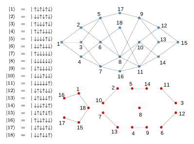
Figure 1: The $F_{5}+F_{7}=18$ Fock states for $L=6$ and their numbering shown in left panel. The right panel shows the connectivity graphs of $H_{\mathrm{PXP}}$ (in blue) and $H_{3}$ (in red) respectively.

These dynamically disconnected sectors lead to a rich fragmented structure of the Hilbert space for $H_{3}$ as we will describe in the rest of the paper. The fragmentation of the Hamiltonian is schematically shown in Fig. 2 where the fragments in the top left quadrant (quadrants marked by blue dotted lines) have dimension $2^{n}\times 2^{n}$ with $n$ being an integer and ranging from $1$ to $n_{0}\sim L/5$. These fragments represent bubble states with strictly localized quasiparticles (hence, a real space description being appropriate). Due to the strict localization property, all eigenstates of any bubble type fragment of size $2^{n}\times 2^{n}$ can be computed. The bottom right quadrant shows some of the analytically tractable states with mobile quasiparticles that are more appropriately written in the momentum basis. In the bottom right quadrant (Fig. 2), we have schematically shown an example of primary fragmentation in momentum space which leads to a $2\times 2$ matrix (indicated in light green with the corresponding matrix for $H_{3}$ written out).

We have also schematically shown examples of a secondary fragmentation mechanism due to specific linear combinations of the basis states whereby a primary fragment (indicated by light green) splits up into two or more secondary fragments (indicated by dark green). Some of these secondary fragments have a fixed dimension (e.g., a $2\times 2$ example shown in Fig. 2 with the corresponding matrix for $H_{3}$ explicitly indicated) that does not scale with increasing system size. This feature makes them analytically tractable even for large $L$. The non-bubble fragments whose dimensions scale with the system size do not seem to have any simple representation of the corresponding high-energy eigenstates in terms of quasiparticles; it is likely that such states satisfy ETH when $L\gg 1$.

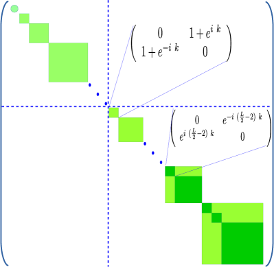
Figure 2: The Hamiltonian structure and the associated fragmentation is schematically shown here. The fragments in the top left quadrant (quadrants indicated by the blue dotted lines) are bubble type fragments whose sizes range from $1\times 1$ to $2^{n_{0}}\times 2^{n_{0}}$ where $n_{0}\sim L/5$. Each of these bubble fragments can be completely diagonalized due to the strictly localized nature of quasiparticles in such states. The non-bubble fragments in the bottom right quadrant are more appropriately expressed in the momentum basis. A $2\times 2$ non-bubble fragment (with the explicit expression for $H_{3}$ shown) is indicated. Some bigger non-bubble fragments (indicated in light green) split up into smaller secondary fragments (indicated in dark green) after a further basis transformation involving a fixed number of basis states. Some of these secondary fragments, therefore, have a fixed dimension with increasing system size. One such $2\times 2$ secondary fragment and the corresponding expression of $H_{3}$ is indicated above.

To further contrast the difference between the spectrum of $H_{3}$ (Eq. 1) and $H_{\mathrm{PXP}}$ (Eq. LABEL:Hpxpdef), we calculate the bipartite entanglement entropy $S_{L/2}$ for $L=28$ in the sector with zero momentum ($k=0$) and spatial inversion symmetry ($I=+1$) for both the models. The bipartite entanglement entropy is given by

$$S_{L/2}=-\mathrm{Tr}[\rho_{A}\ln\rho_{A}]$$ (6)

for each eigenstate $|\Psi\rangle$ where $\rho_{A}=\mathrm{Tr}_{B}|\Psi\rangle\langle\Psi|$ represents the reduced density matrix. Here $\rho_{A}$ is computed by partitioning the one-dimensional chain into two equal halves $A$ and $B$. While typical high-energy eigenstates are expected to show a volume law scaling of $S_{L/2}\sim L$, anomalous high-energy eigenstates usually have much smaller values of $S_{L/2}$. While the bipartite entanglement entropy for $H_{\mathrm{PXP}}$ (Fig. 3 (top right panel)) shows the characteristic scar states of the PXP model as outliers of $S_{L/2}$ that are almost equally spaced in energy, its behavior for $H_{3}$ (Fig. 3 (top left panel)) is markedly different. The latter shows the presence of many more anomalous eigenstates at both integer as well as non-integer eigenvalues. In fact, an entanglement gap seems to emerge in Fig. 3(top left panel) which separates the low and high entanglement entropy eigenstates and this gap should become more pronounced with increasing $L$. It is also clear by comparing both the top panels in Fig. 3 that just like the PXP model, the bulk of the states have large volume-law entanglement in the spectrum of $H_{3}$ (the density of states is shown using the same color map in both panels where warmer color indicates higher density of states) indicating the non-integrable nature of the model. In fact, $S_{L/2}$ approaches a value close to the average entanglement entropy, $S_{\mathrm{Page}}=\ln(\mathcal{D}_{L/2})-\frac{1}{2}$ of pure random states Page where $\mathcal{D}_{L/2}$ is the Hilbert space dimension of A (B), for the mid-spectrum eigenstates in both the top panels of Fig. 3.

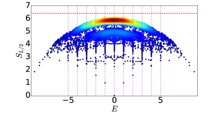
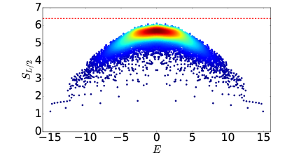
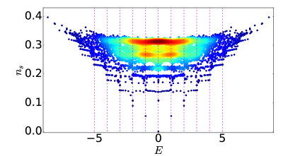
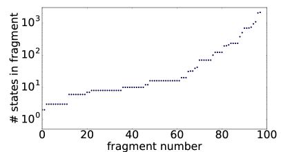
Figure 3: The bipartite entanglement entropy with equal partitions, $S_{L/2}$, shown for all energy eigenstates in the sector with zero momentum and spatial inversion symmetry for $L=28$ in the top panels. The top left panel shows data for $H_{3}$ while the top right panel correspond to $H_{\mathrm{PXP}}$. The horizontal dotted line indicates the average entanglement entropy, $S_{\mathrm{Page}}$, of random pure states in both the top panels. The bottom left panel shows the expectation value of the operator $n_{s}=\sum_{j=1}^{L}(\sigma_{j}^{z}+1)/(2L)$ for the eigenstates of $H_{3}$. The density of states is indicated by the same color map in all three panels where warmer color corresponds to higher density of states. Additionally, dotted vertical lines indicate integer values of $E$ for the top left and bottom left panels. The bottom right panel shows the number of primary fragments induced by $H_{3}$ and their dimensions for the zero momentum and spatial inversion symmetry for $L=28$.

The bottom left panel of Fig. 3 shows the expectation value of the operator $n_{s}=\sum_{j=1}^{L}(\sigma^{z}_{j}+1)/(2L)$ for all the eigenstates of $H_{3}$ at $L=28$ with $k=0$ and $I=+1$ which again highlights that several of the high-energy eigenstates do not seem to satisfy ETH. The bottom right panel of Fig. 3 shows the variations in the sizes of the different (primary) fragments that arise for this symmetry sector with the smallest fragment being $1\times 1$ and the largest being $2125\times 2125$. Lastly, analyzing the data for both the models at $L=28$ with $k=0,I=+1$ clearly shows that while $H_{\mathrm{PXP}}$ does not show any residual degeneracy in the spectrum apart from the zero modes, the spectrum of $H_{3}$ shows exact degeneracies even at non-zero integer values (indicated by dotted vertical lines in Fig. 3 (top left and bottom left panels)).

III Construction of bubble eigenstates

There is a simple class of exact eigenstates that we can write explicitly for $H_{3}$ for any $L$, where these have integer energies and also satisfy strict area law scaling of entanglement entropy in the thermodynamic limit. Let us start with the Fock state with all $S^{z}=\downarrow$. This state is annihilated by $H_{3}$ and is, therefore, an “inert” state which forms a $1\times 1$ fragment in the Hilbert space. Interestingly, while earlier models of fragmentation contained an exponentially large number of inert states for a given system size, this one-dimensional model only contains one such state.

Taking the inert state as a reference state, let us now choose a arbitrary site $i$ and change the corresponding spin to $S_{i}^{z}=\uparrow$. Importantly, this particular Fock state is only connected to one other Fock state in the Hilbert space under the action of $H_{3}$ leading to a $2\times 2$ fragment. Looking at both the Fock states, only the $(i-1,i,i+1)$ spins can differ from the reference state and we denote these two types of building blocks of three adjacent spins as

$$\boxed{X_{1,i}} = \boxed{\uparrow_{i-1}\downarrow_{i}\uparrow_{i+1}}$$

$$\boxed{X_{2,i}} = \boxed{\downarrow_{i-1}\uparrow_{i}\downarrow_{i+1}}.$$ (7)

These blocks are immersed in the background of the rest of the spins being all $\downarrow$ as provided by the reference inert state. Two such states connected under the action of $H_{3}$ are shown below:

$$\cdots\downarrow\downarrow\downarrow\boxed{X_{1,i}}\downarrow\downarrow\downarrow\downarrow\downarrow\downarrow\cdots$$

$$\cdots\downarrow\downarrow\downarrow\boxed{X_{2,i}}\downarrow\downarrow\downarrow\downarrow\downarrow\downarrow\cdots$$ (8)

Placing $n$ such $X_{1,2}$ units, where each of the units is “sufficiently distant” from the others, in the background of the inert state then shows that this Fock state is connected to $2^{n}-1$ other Fock states under $H_{3}$ where any of the $X_{1}$ unit can be changed to a $X_{2}$ unit and vice-versa. The question is how close can these units be for this strict local picture of $X_{1}\leftrightarrow X_{2}$ conversions under $H_{3}$ to hold. For this, it is enough to consider the case where there are two such units inserted in the reference state. Such a consideration shows that if a minimum of two adjacent $S^{z}=\downarrow$ separate the two $X_{1,2}$ units, then the Hilbert space fragment continues to be $4\times 4$ with the four Fock states simply being all combinations of $(X_{1(2),i},X_{1(2),j})$ where $i,j$ denote the central sites of the two units respectively, as shown below:

$$\cdots\downarrow\downarrow\downarrow\boxed{X_{1,i}}\downarrow\downarrow\boxed{X_{1,j}}\downarrow\downarrow\cdots$$

$$\cdots\downarrow\downarrow\downarrow\boxed{X_{1,i}}\downarrow\downarrow\boxed{X_{2,j}}\downarrow\downarrow\cdots$$

$$\cdots\downarrow\downarrow\downarrow\boxed{X_{2,i}}\downarrow\downarrow\boxed{X_{1,j}}\downarrow\downarrow\cdots$$

$$\cdots\downarrow\downarrow\downarrow\boxed{X_{2,i}}\downarrow\downarrow\boxed{X_{2,j}}\downarrow\downarrow\cdots$$ (9)

Thus, bubble Fock states are constructed of various $X_{1(2)}$ immersed in a background of the rest of the spins being $S^{z}=\downarrow$ with the additional constraint that no two $X_{1(2)}$ units have less than two adjacent $\downarrow\downarrow$ separating them. Due to the hard core constraint of at least two consecutive $\downarrow$ spins between any two $X_{1,2}$ units, the maximum value of $n$ (total number of $X_{1,2}$ units in a bubble Fock state) equals $n_{0}=\lfloor L/5\rfloor$ where $\lfloor\mbox{~{}}\rfloor$ denotes the floor function. Thus, for $L\gg 1$, the largest bubble-type Hilbert space fragment equals $2^{L/5}\times 2^{L/5}$.

Given that $H_{3}$ simply converts a $X_{1,j}$ to a $X_{2,j}$ and vice-versa for bubble Fock states, it is straightforward to diagonalize each of these fragments with dimension $2^{n}\times 2^{n}$ where $n=1,2,\cdots,n_{0}$. Denoting $X_{1,j}$ and $X_{2,j}$ as pseudospin-$1/2$ variables with $\tau_{j}^{z}=+1$ and $\tau_{j}^{z}=-1$, the form of $H_{3}$ projected to any $n\neq 0$ bubble type fragment simply equals

$$H_{3,\mathrm{bubble}}=\sum_{j_{b}=1}^{n}\tau_{j_{b}}^{x}$$ (10)

where $j_{b}$ denotes the central sites of the bubbles. This “non-interacting” effective Hamiltonian can be diagonalized for any $n$ to give that a quantum state build out of $n_{1}$ $\boxed{\downarrow_{j-2}X_{j}\downarrow_{j+2}}$ units, $n_{2}$ $\boxed{\downarrow_{j-2}Y_{j}\downarrow_{j+2}}$ units (where $n_{1}+n_{2}=n$) and the rest being $S^{z}=\downarrow$, where

$$X_{j} = \frac{1}{\sqrt{2}}(X_{1,j}+X_{2,j}),\quad{\rm and}\quad Y_{j}=\frac{1}{\sqrt{2}}(X_{1,j}-X_{2,j})$$

are exact eigenstates of $H_{3}$ with eigenvalues $E=n_{1}-n_{2}$. Note that fixing two $\downarrow$ at both sides of $X_{j}$ and $Y_{j}$ automatically ensures that two such units are separated by at least two consecutive $\downarrow$ spins, as required for bubble Fock states. E.g., the four eigenstates obtained by diagonalizing the $4\times 4$ matrix obtained for $n=2$ are as follows:

$$\cdots\downarrow\downarrow\otimes\boxed{\downarrow_{j-2}X_{j}\downarrow_{j+2}}\otimes\boxed{\downarrow_{j+3}X_{j+5}\downarrow_{j+7}}\otimes\downarrow\cdots$$

$$\cdots\downarrow\downarrow\otimes\boxed{\downarrow_{j-2}X_{j}\downarrow_{j+2}}\otimes\boxed{\downarrow_{j+3}Y_{j+5}\downarrow_{j+7}}\otimes\downarrow\cdots$$

$$\cdots\downarrow\downarrow\otimes\boxed{\downarrow_{j-2}Y_{j}\downarrow_{j+2}}\otimes\boxed{\downarrow_{j+3}X_{j+5}\downarrow_{j+7}}\otimes\downarrow\cdots$$

$$\cdots\downarrow\downarrow\otimes\boxed{\downarrow_{j-2}Y_{j}\downarrow_{j+2}}\otimes\boxed{\downarrow_{j+3}Y_{j+5}\downarrow_{j+7}}\otimes\downarrow\cdots$$

Thinking of $X_{j},Y_{j}$ as local quasiparticles of $H_{3}$, the bubble eigenstates have the property that they are composed of strictly localized or immobile quasiparticles and have integer energies. From the construction of the eigenstates, it is evident that these satisfy an area law for entanglement entropy where the bipartite entanglement entropy can only be $S_{L/2}=0$, $\ln 2$ or $2\ln 2$ depending on whether the bipartition intersects zero, one or two $X/Y$ units in spite of being high-energy eigenstates. For example, the bubble eigenstates at $E=0$ are mid-spectrum states owing to the $E$ to $-E$ symmetry of the spectrum of $H_{3}$ and, therefore, violate ETH since such states are expected to have volume law scaling of entanglement entropy.

The number of bubble eigenstates at an integer energy $E=n_{1}-n_{2}$ can be calculated for a given system size from the number of configurations that satisfy the hard core constraint of at least two consecutive $\downarrow$ spins separating any of the $n_{1}$ $X$ and $n_{2}$ $Y$ units on the periodic one-dimensional lattice. In Table. 1, we compare the number of bubble eigenstates at each $E=0,\pm 1,\pm 2,\cdots$ (the number of bubble eigenstates for $E=n$ equals that for $E=-n$ because of the $E$ to $-E$ symmetry of the spectrum) for chains with $L=16,18,20$ with the degeneracy of integer eigenvalues obtained from the exact diagonalization data (ED) (without restricting to any symmetry sector). Comparing the degeneracy of the bubble eigenstates with the integer eigenstates, we see that for $L=16,18,20$, $E=\pm n_{0}$ eigenstates are solely the bubble eigenstates. We conjecture that this property is true for any $L$. In fact, for $L=20$, even the $E=\pm(n_{0}-1)$ eigenstates are all bubble eigenstates. However, the situation is quite different as we move closer to $E=0$ where it is clear that there are a large number of non-bubble eigenstates that have integer eigenvalues as well.

Table 1: The number of bubble eigenstates at integer energies and the number of integer eigenstates obtained from exact diagonalization for chain lengths $L=16,18,20$.

$L=16$	Bubble eigenstates	Exact Diagonalization
$E=+3$ (or $-3$)	$16$	$16$
$E=+2$ (or $-2$)	$56$	$57$
$E=+1$ (or $-1$)	$64$	$132$
$E=0$	$113$	$193$
$L=18$	Bubble eigenstates	Exact Diagonalization
$E=+3$ (or $-3$)	$60$	$60$
$E=+2$ (or $-2$)	$81$	$100$
$E=+1$ (or $-1$)	$198$	$308$
$E=0$	$163$	$348$
$L=20$	Bubble eigenstates	Exact Diagonalization
$E=+4$ (or $-4$)	$5$	$5$
$E=+3$ (or $-3$)	$140$	$140$
$E=+2$ (or $-2$)	$130$	$255$
$E=+1$ (or $-1$)	$440$	$600$
$E=0$	$251$	$709$

While we have not been able to find a closed form expression for the degeneracy of the different bubble eigenstates for an arbitrary $L$, we can still place a lower bound on the degeneracy of such states when $L\gg 1$. Consider a chain of length $L=10m$ where $m$ is an integer. Then, the maximum number of $X/Y$ units that can be accommodated due to the hard core constraints equals $n_{0}=2m$. Ignoring whether a bubble is $X/Y$ type, there are only $5$ distinct ways of placing all the $n_{0}$ bubbles in the chain since each bubble is separated from the neighboring ones by precisely two lattice sites when $L=10m$. To construct a bubble eigenstate with energy $E=2n-n_{0}$, $n$ bubbles need to be made $X$ type and the rest ($n_{0}-n$) $Y$ type which introduces an additional degeneracy of ${n_{0}\choose n}$. Assuming both $n_{0},n\gg 1$, we then get that the degeneracy of bubble eigenstates with energy $E=2n-n_{0}$ (denoted by $\Omega_{B}(n)$ below) is bounded below by

$$\Omega_{B}(n)>5\times 2^{n_{0}}\sqrt{\frac{2}{\pi n_{0}}}\exp\left(2n_{0}\left(x-\frac{1}{2}\right)^{2}\right)$$ (13)

where $n_{0}=L/5$ and $x=n/n_{0}$ for $L\gg 1$. This bound immediately shows that the number of bubble eigenstates is exponentially large in the system size for integer energies that range from $E=0$ to $|E|\sim\mathrm{O}(\sqrt{L})$ while the maximum value of the integer energy $|E|\sim L/5$ when $L\gg 1$. Since the bubble eigenstates satisfy area law scaling of entanglement entropy (with a maximum $S_{L/2}=2\ln(2)$), it is an interesting open question to find how the number of non-bubble integer eigenstates scales with system size and how many of such eigenstates satisfy volume law scaling of entanglement entropy, especially in the neighborhood of $E=0$, given the non-integrable nature of $H_{3}$ and the numerical data presented in Fig. 3 (top left panel).

While the bubble eigenstates have strictly localized quasiparticles, there are other anomalous high-energy excitations for this model which we collectively dub as “non-bubble” eigenstates. These are necessarily composed of mobile excitations and seem to have a more natural description in momentum space. Unlike the bubble eigenstates, we do not claim to have a complete understanding of these special eigenstates. In the next two sections, we describe a class of such non-bubble eigenstates of $H_{3}$.

IV Non-bubble eigenstates with dispersing quasiparticles

The simplest non-bubble eigenstates are composed starting from Fock states with two $X_{2}$ units next to each other with the rest of the spins being $S^{z}=\downarrow$ provided by the (inert) reference state. The action of $H_{3}$ then leads to an effective hopping of these two $X_{2}$ units together either in the forward or backward direction through intermediate Fock states with two consecutive $X_{1},X_{2}$ units that also move forward or backward in the same manner.

$$\cdot\cdot\downarrow\downarrow\boxed{X_{2,j}}\boxed{X_{2,j+3}}\downarrow\downarrow\cdot\cdot\leftrightarrows\cdot\cdot\downarrow\downarrow\boxed{X_{1,j}}\boxed{X_{2,j+3}}\downarrow\downarrow\cdot\cdot\leftrightarrows\cdot\cdot\downarrow\boxed{X_{2,j-1}}\boxed{X_{2,j+2}}\downarrow\downarrow\downarrow\cdot\cdot\leftrightarrows\cdot\cdot\downarrow\boxed{X_{1,j-1}}\boxed{X_{2,j+2}}\downarrow\downarrow\downarrow\cdot\cdot$$

$$\cdot\cdot\downarrow\downarrow\boxed{X_{2,j}}\boxed{X_{2,j+3}}\downarrow\downarrow\cdot\cdot\leftrightarrows\cdot\cdot\downarrow\downarrow\boxed{X_{2,j}}\boxed{X_{1,j+3}}\downarrow\downarrow\cdot\cdot\leftrightarrows\cdot\cdot\downarrow\downarrow\downarrow\boxed{X_{2,j+1}}\boxed{X_{2,j+4}}\downarrow\cdot\cdot\leftrightarrows\cdot\cdot\downarrow\downarrow\downarrow\boxed{X_{2,j+1}}\boxed{X_{1,j+4}}\downarrow\cdot\cdot$$

(14)

Using this observation, we find it convenient to go to momentum space and define the following two basis states:

$$|\Phi_{1,k}\rangle = \frac{1}{\sqrt{L}}\sum_{j=1}^{L}\exp(ikj)T^{j}|\uparrow\downarrow\downarrow\uparrow\underbrace{\downarrow\downarrow\cdots\downarrow\downarrow}_{L-4}\rangle$$

$$|\Phi_{2,k}\rangle = \frac{1}{\sqrt{L}}\sum_{j=1}^{L}\exp(ikj)T^{j}|\uparrow\downarrow\uparrow\downarrow\uparrow\underbrace{\downarrow\cdots\downarrow\downarrow}_{L-5}\rangle$$ (15)

where $T$ represents a global translation by one lattice unit and the momentum $k=2\pi n/L$ where $n=0,1,2,\cdots,L-1$. The spins in $\underbrace{\downarrow\cdots\downarrow}$ are all assumed to be $\downarrow$. These basis states then define a $2\times 2$ fragment in momentum space at each $k$ because

$$H_{3}|\Phi_{1,k}\rangle=(1+\exp(ik))|\Phi_{2,k}\rangle.$$ (16)

Diagonalizing the $2\times 2$ matrix leads to the following exact eigenenergies and eigenvectors:

$$E_{\pm}(k) = \pm 2\cos k/2$$

$$|\Psi_{\pm}(k)\rangle = \frac{\exp(-ik/2)|\Phi_{1,k}\rangle\pm|\Phi_{2,k}\rangle}{\sqrt{2}}$$ (17)

This leads to two dispersive bands composed of a total of $2L$ anomalous eigenvectors at high energies. Thus, we have obtained a very simple class of exact eigenstates with irrational energies in general for any $L\gg 1$. E.g., for any $L\geq 8$ which is a multiple of four, such that $k=\pi/2$ is allowed, these eigenstates have energies $E=\pm\sqrt{2}$ at that particular momentum. In fact, for $L=16$, such a non-bubble eigenstate with $E=2(-2)$ state at $k=0$ provides the missing eigenstate apart from the $56$ bubble eigenstates when we compare with the ED results (Table. 1). Moreover, these states have the symmetry $E_{\pm}(2\pi-k)=E_{\mp}(k)$. Thus they intersect at $k=\pi$ leading to two zero energy non-bubble eigenstates. In Fig. 4, we show the presence of these two dispersive bands of eigenstates in momentum space for a chain of $L=18$ after resolving the ED data in momentum $k$.

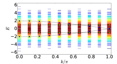
Figure 4: The momentum resolved energy spectrum for $L=18$ where the color map indicates the density of states. The non-bubble eigenstates that lead to two dispersive bands and two flat bands in momentum space respectively are highlighted as blue and green dots respectively. The dashed lines are a guide to the eye. The color map indicates the momentum resolved density of states. Warmer color corresponds to higher density of states.

V Secondary fragmentation of the Hilbert space

We now point out a novel secondary fragmentation mechanism, which did not appear in previous models to the best of our knowledge, whereby certain specific linear combinations of a fixed number of basis states contained in a large primary fragment (whose dimension keeps increasing with system size) turns out to be orthogonal to all other vectors inside the fragment. In addition, they also form a closed subspace under the action of $H_{3}$ leading to a smaller emergent fragment of a fixed dimension in the Hilbert space. We note that though most of the eigenvalues inside the larger primary fragments are irrational in nature, as expected for a non-integrable model, diagonalization of these smaller secondary fragments gives integer eigenvalues. These non-bubble states with integer eigenvalues exist inside the larger primary fragments of all momentum sectors and their number increases with increasing system size. We discuss two such examples of exact non-bubble eigenstates that emerge from this mechanism below.

V.1 Secondary fragmentation in $k=0,I=+1$

We first discuss the formation of an exact state inside the largest primary fragment of $k=0,I=+1$. We note here that the state $(|{\mathbb{Z}}_{2}\rangle+|{\bar{\mathbb{Z}}}_{2}\rangle)/\sqrt{2}$ belongs to this fragment for $L=10,16,22,28\cdots$; however for other $L$, this is not the case. To this end we consider the following four basis states with $k=0$, $I=+1$ defined as

$$|v_{1}\rangle = \frac{1}{\sqrt{2L}}\sum_{j=1}^{L}T^{j}(1+I)|\uparrow\downarrow\downarrow\uparrow\downarrow\uparrow\downarrow\downarrow\downarrow\uparrow\underbrace{\downarrow\cdots\downarrow}_{L-10}\rangle$$

$$|v_{2}\rangle = \frac{1}{\sqrt{2L}}\sum_{j=1}^{L}T^{j}(1+I)|\uparrow\downarrow\uparrow\downarrow\downarrow\uparrow\downarrow\downarrow\downarrow\downarrow\uparrow\underbrace{\downarrow\cdots\downarrow}_{L-11}\rangle$$

$$|v_{3}\rangle = \frac{1}{\sqrt{2L}}\sum_{j=1}^{L}T^{j}(1+I)|\uparrow\downarrow\uparrow\downarrow\downarrow\uparrow\downarrow\uparrow\downarrow\downarrow\uparrow\underbrace{\downarrow\cdots\downarrow}_{L-11}\rangle$$

$$|v_{4}\rangle = \frac{1}{\sqrt{2L}}\sum_{j=1}^{L}T^{j}(1+I)|\uparrow\downarrow\uparrow\downarrow\downarrow\uparrow\downarrow\downarrow\downarrow\uparrow\downarrow\uparrow\underbrace{\downarrow\cdots\downarrow}_{L-12}\rangle$$

Remarkably, the following linear combinations

$$|\psi_{a}\rangle = \frac{1}{\sqrt{2}}(|v_{1}\rangle-|v_{2}\rangle)$$

$$|\psi_{b}\rangle = \frac{1}{\sqrt{2}}(|v_{3}\rangle-|v_{4}\rangle)$$ (19)

are orthogonal to the rest of the states in the fragment and are closed under the action of $H_{3}$ since $H_{3}|\psi_{a,b}\rangle=-|\psi_{b,a}\rangle$. To see why this is the case, we first note that the action of $H_{3}$ on $|v_{1}\rangle$ and $|v_{2}\rangle$ leads to states with three up-spins that are clearly outside the subspace described above. Similarly $H_{3}$ acting on $|v_{3}\rangle$ and $|v_{4}\rangle$ leads to states with six up-spins. The particular linear combinations chosen in Eq. 19 cancel the amplitude of these states. Moreover $H_{3}$ acting on $|v_{1}\rangle$ and $|v_{2}\rangle$ also generate five up-spin states other than $|v_{3}\rangle$ and $|v_{4}\rangle$; the amplitude of these states also cancel with the linear combination mentioned above. This leads to this secondary fragmentation for any $L\geq 16$. Diagonalizing this $2\times 2$ fragment then gives the following eigenstates

$$\frac{1}{\sqrt{2}}(|\psi_{a}\rangle\pm|\psi_{b}\rangle)$$ (20)

with $E=\mp 1$.

V.2 Non-bubble eigenstates with flat bands

We also find a class of high-energy eigenstates in this model that form flat bands in momentum space. The relevant basis states in momentum space are as follows

$$|w_{1}\rangle = \frac{1}{\sqrt{L}}\sum_{j=1}^{L}\exp(ikj)T^{j}|\uparrow\underbrace{\downarrow\cdots\downarrow}_{\frac{L}{2}-4}\uparrow\downarrow\uparrow\downarrow\downarrow\uparrow\underbrace{\downarrow\cdots\downarrow}_{\frac{L}{2}-3}\rangle$$

$$|w_{2}\rangle = \frac{1}{\sqrt{L}}\sum_{j=1}^{L}\exp(ikj)T^{j}|\uparrow\downarrow\downarrow\uparrow\downarrow\uparrow\underbrace{\downarrow\cdots\downarrow}_{\frac{L}{2}-4}\uparrow\underbrace{\downarrow\cdots\downarrow}_{\frac{L}{2}-3}\rangle$$

$$|w_{3}\rangle = \frac{1}{\sqrt{L}}\sum_{j=1}^{L}\exp(ikj)T^{j}|\uparrow\downarrow\uparrow\underbrace{\downarrow\cdots\downarrow}_{\frac{L}{2}-5}\uparrow\downarrow\uparrow\downarrow\downarrow\uparrow\underbrace{\downarrow\cdots\downarrow}_{\frac{L}{2}-4}\rangle$$

$$|w_{4}\rangle = \frac{1}{\sqrt{L}}\sum_{j=1}^{L}\exp(ikj)T^{j}|\uparrow\downarrow\downarrow\uparrow\downarrow\uparrow\underbrace{\downarrow\cdots\downarrow}_{\frac{L}{2}-5}\uparrow\downarrow\uparrow\underbrace{\downarrow\cdots\downarrow}_{\frac{L}{2}-4}\rangle$$

Note that $\langle w_{1}|H_{3}|w_{3}\rangle=\exp(-ik)$ and $\langle w_{2}|H_{3}|w_{4}\rangle=1$. An appropriate linear combination of $|w_{i}\rangle$ ($i=1,2$ and $i=3,4$) can be found following the same principle described in the previous subsection; these linear combinations are

$$|\chi_{a}\rangle = \frac{1}{\sqrt{2}}\left(|w_{1}\rangle-e^{-i\left(\frac{L}{2}-2\right)k}|w_{2}\rangle\right)$$

$$|\chi_{b}\rangle = \frac{1}{\sqrt{2}}\left(|w_{4}\rangle-e^{-i\left(\frac{L}{2}+1\right)k}|w_{3}\rangle\right).$$ (22)

Note that, whereas the states in the previous example belong to $I=+1$ sector, the basis states in Eq. (22) belong to $I=-1$ sector for $k=0,\pi$ sectors. $H_{3}$ has the following representation in the basis of $|\chi_{a,b}\rangle$

$$\left(\begin{array}[]{cc}0&e^{i\left(\frac{L}{2}-2\right)k}\\ e^{-i\left(\frac{L}{2}-2\right)k}&0\end{array}\right)$$ (25)

and thus leads to a $2\times 2$ fragment due to a secondary fragmentation. On diagonalization, we obtain two eigenvectors at each $k$ as follows

$$\frac{1}{\sqrt{2}}(\pm e^{i\left((L/2)-2\right)k}|\chi_{a}\rangle+|\chi_{b}\rangle)$$ (26)

with eigenvalues $E=\pm 1$ for all $k$, thus realizing two perfectly flat bands of anomalous eigenstates in momentum space. These flat bands are shown in Fig. 4 for $L=18$ using momentum-resolved ED results.

VI Adding non-commuting interactions to the model

We now explore the effects of adding two non-commuting interactions to the $H_{3}$ model respectively (while the constrained Hilbert space still remains the same). The first case will be that of a staggered magnetic field while the second will be the PXP Hamiltonian.

VI.1 Staggered magnetic field term

The staggered magnetic field corresponds to a Hamiltonian of the form

$$H_{s}=\sum_{j=1}^{L}(-1)^{j}\sigma_{j}^{z}.$$ (27)

$H_{s}$ has some properties that are worth pointing out. Unlike $H_{3}$ or $H_{\mathrm{PXP}}$, $H_{s}$ commutes with $Q$ (Eq. 5) and anticommutes with the spatial inversion symmetry $I$. Furthermore, $H_{s}$ anticommutes with the operator $C$ defined as

$$C=\prod_{j=1}^{L/2}\left(\sigma^{z}_{2j-1}+\sigma^{z}_{2j}\right)$$ (28)

which ensures that every eigenstate $|E\rangle$ with energy $E$ has a partner $C|E\rangle$ with energy $-E$. Together with $\{H,QI\}=0$, this implies the presence of an exponentially large number of zero modes in the spectrum of $H_{s}$. These zero modes are simply Fock states in the constrained Hilbert space with the same number of $\uparrow$ spins (and hence $\downarrow$ spins) on the even and odd sites of the chain.

The model that we consider now has the following Hamiltonian

$$H_{\Delta} = H_{3}+\frac{\Delta}{2}H_{s}$$

$$= \sum_{j=1}^{L}(\tilde{\sigma}_{j}^{+}\tilde{\sigma}_{j-1}^{-}\tilde{\sigma}_{j+1}^{-}+\mathrm{H.c.})+\frac{\Delta}{2}\sum_{j=1}^{L}(-1)^{j}\sigma_{j}^{z}$$

It is immediately clear that the connectivity graphs of $H_{3}$ (Fig. 1) and $H_{\Delta}$ are identical in the basis of the Fock states since $H_{s}$ is a purely diagonal term in this basis. Thus, $H_{\Delta}$ continues to show Hilbert space fragmentation in spite of the fact that $H_{s}$ does not commute with $H_{3}$. Like $H_{3}$ and $H_{s}$, the spectrum of $H_{\Delta}$ also has an $E\rightarrow-E$ symmetry. Furthermore, since $H_{\Delta}$ anticommutes with the combination $QI$, it also harbors an exponentially large number of mid-spectrum zero modes.

We first calculate the degeneracy of zero modes of $H_{\Delta}$ numerically using ED for chain lengths $L=16,18,20$ when $\Delta=0$, $\Delta\neq 0$, and $\Delta\rightarrow\infty$ (non-interacting limit) and give the numbers in Table. 2. We also give a lower bound for the number of zero modes at $\Delta\neq 0$ in the same table which we will justify below. Interestingly, the numerics indicate that the number of zero modes is independent of $\Delta$ as long as it is finite and non-zero.

Table 2: The number of zero modes obtained from exact diagonalization shown for three chain lengths $L=16,18,20$ for $\Delta=0$, $\Delta\neq 0$, and $\Delta\rightarrow\infty$. A lower bound is also given for the number of zero modes for $\Delta\neq 0$.

$L$	$\Delta=0$	$\Delta\neq 0$	Lower bound	$\Delta\rightarrow\infty$
$16$	$193$	$77$	$65$	$313$
$18$	$348$	$180$	$91$	$778$
$20$	$709$	$247$	$151$	$1941$

We first consider bubble type fragments with $n$ bubbles. The case of $n=0$ is the simplest. The inert state of $H_{3}$ continues to be the lone inert state of $H_{\Delta}$ and is a simultaneous eigenket of both the non-commuting terms for any $L$. We now follow the same logic used to derive Eq. 10 for $n\neq 0$ and again denote $X_{1,j}$ and $X_{2,j}$ as pseudospin-$1/2$ variables with $\tau_{j}^{z}=+1$ and $\tau_{j}^{z}=-1$. Here, it is useful to note that the energy of a bubble Fock state with respect to $H_{s}$ can be written in the form $E_{s}=\sum_{j}(E_{j}(X_{1,j})+E_{j}(X_{2,j}))$ where $E_{j}(X_{1,j})$ equals $-4(4)$ if $j$ is even (odd) and $E_{j}(X_{2,j})$ equals $2(-2)$ if $j$ is even (odd) with $X_{1,j}(X_{2,j})$ representing a $\uparrow_{j-1}\downarrow_{j}\uparrow_{j+1}(\downarrow_{j-1}\uparrow_{j}\downarrow_{j+1})$ unit of three consecutive spins as defined in Eq. 7. Then, the form of $H_{\Delta}$ projected to any $n\neq 0$ bubble type fragment simply equals

$$H_{\Delta,\mathrm{bubble}} = \sum_{j_{b}=1}^{n}\tau_{j_{b}}^{x}+\frac{3\Delta}{2}(\sum_{j_{b}=1}^{n}(-1)^{j_{b}}\tau_{j_{b}}^{z})+\frac{\Delta}{2}(n_{\mathrm{odd}}-n_{\mathrm{even}})$$ (30)

$$= \frac{1}{2}\sqrt{4+9\Delta^{2}}\left(\sum_{j_{b}=1}^{n}\hat{h}\cdot\tilde{\mathbf{\tau}}_{j_{b}}\right)+\frac{\Delta}{2}(n_{\mathrm{odd}}-n_{\mathrm{even}})$$

where $j_{b}$ denotes the central sites of the bubbles with $n_{\mathrm{odd}}$ ($n_{\mathrm{even}}$) equalling the number of bubbles centered on odd (even) sites of the lattice. The second line of Eq. 30 has been obtained from the first line by using the transformation $\tilde{\tau}_{j}^{y,z}=-\tau_{j}^{y,z}$ for any $j$ that is odd. The unit vector $\hat{h}$ equals $(2/\sqrt{4+9\Delta^{2}},0,3\Delta/\sqrt{4+9\Delta^{2}})$. Since this “non-interacting” effective Hamiltonian cannot entangle the $\tilde{\tau}_{j}$ variables, all the eigenstates of $H_{\Delta}$ obtained from the bubble fragments continue to have a strict area law scaling of entanglement entropy even when $L\gg 1$.

Comparing Eq. 30 with Eq. 10, we immediately see that for any fragment with an equal number of bubbles centered on even and odd sites of the lattice, the eigenvalues of $H_{\Delta}$ and $H_{3}$ are just related by a scale factor that equals $(\sqrt{4+9\Delta^{2}})/2$. In particular, the degeneracy of the zero modes obtained from such fragments remain unchanged with $\Delta$ even though the eigenvectors themselves change. In contrast, the degeneracy of zero modes drops to zero for bubble type fragments where the $n$ bubbles are distributed unequally between even and odd sites of the chain when $\Delta$ is changed from zero to any non-zero value because of the $(\Delta/2)(n_{\mathrm{odd}}-n_{\mathrm{even}})$ term in Eq. 30. We have used these two facts to obtain a lower bound on the number of zero modes in $H_{\Delta}$ in Table. 2.

We now explicitly look at the cases with $n=2$ and $n=4$ from which we see that not only does the number of zero modes for such fragments stay independent of $\Delta$ but the zero modes come in two varieties – those that are simultaneous eigenkets of $H_{s}$ and $H_{3}$ and those that are not. The eigenfunctions of the former class of zero modes stay unchanged with $\Delta$ while the latter class of zero modes change as $\Delta$ is varied. Below, we will assume that half of these units are centered on even sites while the other half are centered on odd sites of the chain.

$n=2$ case: Consider the following four bubble-type Fock states

$$|b_{1}\rangle = \cdots\downarrow\downarrow\boxed{X_{2,i}}\downarrow\cdots\downarrow\boxed{X_{1,j}}\downarrow\downarrow\cdots(E_{s}=+6)$$

$$|b_{2}\rangle = \cdots\downarrow\downarrow\boxed{X_{2,i}}\downarrow\cdots\downarrow\boxed{X_{2,j}}\downarrow\downarrow\cdots(E_{s}=0)$$

$$|b_{3}\rangle = \cdots\downarrow\downarrow\boxed{X_{1,i}}\downarrow\cdots\downarrow\boxed{X_{1,j}}\downarrow\downarrow\cdots(E_{s}=0)$$

$$|b_{4}\rangle = \cdots\downarrow\downarrow\boxed{X_{1,i}}\downarrow\cdots\downarrow\boxed{X_{2,j}}\downarrow\downarrow\cdots(E_{s}=-6)$$

(31)

where we choose $i$ to be an even site and $j$ an odd site on the chain. These form a $4\times 4$ fragment for $H_{\Delta}$ at any $\Delta$ and are eigenstates of $H_{\Delta}$ when $\Delta\rightarrow\infty$. When $\Delta=0$, the eigenstates are instead bubble-type eigenstates of $H_{3}$ (as discussed Sec. III) with energies $+2$ (with degeneracy $1$), $0$ (with degeneracy $2$) and $-2$ (with degeneracy $1$). The (unnormalized) eigenvectors for the two zero modes are as follows:

$$|z_{1}\rangle = |b_{2}\rangle-|b_{3}\rangle$$

$$|z_{2}\rangle = (|b_{1}\rangle-|b_{4}\rangle)-3\Delta|b_{2}\rangle.$$ (32)

While $|z_{1}\rangle$ is composed of the zero modes of $H_{s}$ and is, therefore, a simultaneous eigenket of $H_{3}$ and $H_{s}$, $|z_{2}\rangle$ is not an eigenket of $H_{3}$ or $H_{s}$ but only of $H_{\Delta}$.

$n=4$ case: Consider the following sixteen bubble-type Fock states

$$|c_{1}\rangle = \cdots\downarrow\downarrow\boxed{X_{2,i}}\downarrow\cdots\downarrow\boxed{X_{2,j}}\downarrow\cdots\downarrow\boxed{X_{1,l}}\downarrow\cdots\downarrow\boxed{X_{1,m}}\downarrow\downarrow\cdots(E_{s}=+12)$$

$$|c_{2}\rangle = \cdots\downarrow\downarrow\boxed{X_{2,i}}\downarrow\cdots\downarrow\boxed{X_{2,j}}\downarrow\cdots\downarrow\boxed{X_{1,l}}\downarrow\cdots\downarrow\boxed{X_{2,m}}\downarrow\downarrow\cdots(E_{s}=+6)$$

$$|c_{3}\rangle = \cdots\downarrow\downarrow\boxed{X_{2,i}}\downarrow\cdots\downarrow\boxed{X_{2,j}}\downarrow\cdots\downarrow\boxed{X_{2,l}}\downarrow\cdots\downarrow\boxed{X_{1,m}}\downarrow\downarrow\cdots(E_{s}=+6)$$

$$|c_{4}\rangle = \cdots\downarrow\downarrow\boxed{X_{1,i}}\downarrow\cdots\downarrow\boxed{X_{2,j}}\downarrow\cdots\downarrow\boxed{X_{1,l}}\downarrow\cdots\downarrow\boxed{X_{1,m}}\downarrow\downarrow\cdots(E_{s}=+6)$$

$$|c_{5}\rangle = \cdots\downarrow\downarrow\boxed{X_{2,i}}\downarrow\cdots\downarrow\boxed{X_{1,j}}\downarrow\cdots\downarrow\boxed{X_{1,l}}\downarrow\cdots\downarrow\boxed{X_{1,m}}\downarrow\downarrow\cdots(E_{s}=+6)$$

$$|c_{6}\rangle = \cdots\downarrow\downarrow\boxed{X_{1,i}}\downarrow\cdots\downarrow\boxed{X_{1,j}}\downarrow\cdots\downarrow\boxed{X_{1,l}}\downarrow\cdots\downarrow\boxed{X_{1,m}}\downarrow\downarrow\cdots(E_{s}=0)$$

$$|c_{7}\rangle = \cdots\downarrow\downarrow\boxed{X_{1,i}}\downarrow\cdots\downarrow\boxed{X_{2,j}}\downarrow\cdots\downarrow\boxed{X_{1,l}}\downarrow\cdots\downarrow\boxed{X_{2,m}}\downarrow\downarrow\cdots(E_{s}=0)$$

$$|c_{8}\rangle = \cdots\downarrow\downarrow\boxed{X_{1,i}}\downarrow\cdots\downarrow\boxed{X_{2,j}}\downarrow\cdots\downarrow\boxed{X_{2,l}}\downarrow\cdots\downarrow\boxed{X_{1,m}}\downarrow\downarrow\cdots(E_{s}=0)$$

$$|c_{9}\rangle = \cdots\downarrow\downarrow\boxed{X_{2,i}}\downarrow\cdots\downarrow\boxed{X_{1,j}}\downarrow\cdots\downarrow\boxed{X_{2,l}}\downarrow\cdots\downarrow\boxed{X_{1,m}}\downarrow\downarrow\cdots(E_{s}=0)$$

$$|c_{10}\rangle = \cdots\downarrow\downarrow\boxed{X_{2,i}}\downarrow\cdots\downarrow\boxed{X_{1,j}}\downarrow\cdots\downarrow\boxed{X_{1,l}}\downarrow\cdots\downarrow\boxed{X_{2,m}}\downarrow\downarrow\cdots(E_{s}=0)$$

$$|c_{11}\rangle = \cdots\downarrow\downarrow\boxed{X_{2,i}}\downarrow\cdots\downarrow\boxed{X_{2,j}}\downarrow\cdots\downarrow\boxed{X_{2,l}}\downarrow\cdots\downarrow\boxed{X_{2,m}}\downarrow\downarrow\cdots(E_{s}=0)$$

$$|c_{12}\rangle = \cdots\downarrow\downarrow\boxed{X_{1,i}}\downarrow\cdots\downarrow\boxed{X_{1,j}}\downarrow\cdots\downarrow\boxed{X_{1,l}}\downarrow\cdots\downarrow\boxed{X_{2,m}}\downarrow\downarrow\cdots(E_{s}=-6)$$

$$|c_{13}\rangle = \cdots\downarrow\downarrow\boxed{X_{1,i}}\downarrow\cdots\downarrow\boxed{X_{1,j}}\downarrow\cdots\downarrow\boxed{X_{2,l}}\downarrow\cdots\downarrow\boxed{X_{1,m}}\downarrow\downarrow\cdots(E_{s}=-6)$$

$$|c_{14}\rangle = \cdots\downarrow\downarrow\boxed{X_{1,i}}\downarrow\cdots\downarrow\boxed{X_{2,j}}\downarrow\cdots\downarrow\boxed{X_{2,l}}\downarrow\cdots\downarrow\boxed{X_{2,m}}\downarrow\downarrow\cdots(E_{s}=-6)$$

$$|c_{15}\rangle = \cdots\downarrow\downarrow\boxed{X_{2,i}}\downarrow\cdots\downarrow\boxed{X_{1,j}}\downarrow\cdots\downarrow\boxed{X_{2,l}}\downarrow\cdots\downarrow\boxed{X_{2,m}}\downarrow\downarrow\cdots(E_{s}=-6)$$

$$|c_{16}\rangle = \cdots\downarrow\downarrow\boxed{X_{1,i}}\downarrow\cdots\downarrow\boxed{X_{1,j}}\downarrow\cdots\downarrow\boxed{X_{2,l}}\downarrow\cdots\downarrow\boxed{X_{2,m}}\downarrow\downarrow\cdots(E_{s}=-12)$$ (33)

where we choose $i$, $j$ to be an even sites and $l$, $m$ to be odd sites on the chain. These Fock states form a $16\times 16$ fragment for $H_{\Delta}$ and are eigenstates of $H_{\Delta}$ when $\Delta\rightarrow\infty$. When $\Delta=0$, the eigenstates of $H_{\Delta}$ are instead bubble-type eigenstates (as discussed Sec. III) with energies $+4$ (with degeneracy $1$), $+2$ (with degeneracy $4$), $0$ (with degeneracy $6$), $-2$ (with degeneracy $4$) and $-4$ (with degeneracy $1$). Writing the (unnormalized) eigenvectors for the zero modes:

$$|z_{1}\rangle = |c_{6}\rangle-|c_{7}\rangle-|c_{9}\rangle+|c_{11}\rangle$$

$$|z_{2}\rangle = |c_{7}\rangle-|c_{8}\rangle+|c_{9}\rangle-|c_{10}\rangle$$

$$|z_{3}\rangle = (|c_{3}\rangle-|c_{4}\rangle+|c_{12}\rangle-|c_{15}\rangle)+3\Delta(|c_{6}\rangle-|c_{9}\rangle)$$

$$|z_{4}\rangle = (|c_{3}\rangle-|c_{5}\rangle+|c_{12}\rangle-|c_{14}\rangle)+3\Delta(|c_{6}\rangle-|c_{8}\rangle)$$

$$|z_{5}\rangle = (|c_{2}\rangle-|c_{3}\rangle-|c_{12}\rangle+|c_{13}\rangle)-3\Delta(|c_{7}\rangle-|c_{8}\rangle)$$

$$|z_{6}\rangle = (|c_{1}\rangle-|c_{16}\rangle)-3\Delta(|c_{2}\rangle-|c_{3}\rangle+|c_{4}\rangle-|c_{5}\rangle-2|c_{12}\rangle)+[9\Delta^{2}(|c_{6}\rangle+|c_{7}\rangle-|c_{8}\rangle)-(|c_{7}\rangle+|c_{9}\rangle)]$$ (34)

We also see a similar structure in the eigenvectors of the zero modes when compared to the $n=2$ case. While $|z_{1,2}\rangle$ are simultaneous eigenkets of both $H_{3}$ and $H_{s}$ since these are entirely composed of the zero modes of $H_{s}$, this is not the case for the rest of the zero modes which keep changing as a function of $\Delta$.

For a general $n$, the total number of such zero modes in a given bubble fragment can be estimated as follows. First, we note from the previous discussion that the number of such zero energy states are same as the number of zero energy eigenstates of $H_{s}$. Thus we need to estimate the number of such zero energy states for arbitrary $n$. To this end, we note that for $E_{s}=0$, we need to have equal number of $X_{1,j}$ and $X_{2,j}$ bubbles on even and odd sites. Let us then consider a configuration where there are $p$ $X_{1,j}$ bubbles on even sublattice. This implies that one must have $(n/2-p)$ $X_{2,j}$ bubbles on even sublattice. Also such a configuration can be realized in ${}^{n/2}C_{p}\,\,^{n/2}C_{n/2-p}$ ways. Since $p$ can range from $0$ to $n/2$. we find the total number of zero energy states for $n$ bubble states to be

$$N_{0} = \sum_{p=0}^{n/2}\left({}^{n/2}C_{p}\right)^{2}=\left({}^{n}C_{n/2}\right)$$ (35)

where we have used the relation ${}^{n/2}C_{p}=^{n/2}C_{n/2-p}$. Eq. 35 correctly estimate $N_{0}=2(6)$ for $n=2(4)$ as obtained earlier. We note that this counting assumes $L\gg n$ and does not estimate the number of ways $n$ can be realized on a chain of length $L$. Further, the equality between zero energy of eigenstates and $H_{s}$ and $H_{\Delta}$ only pertains to their number; the states, as shown above in Eqs. 32 and 34, are indeed distinct. The number of simultaneous zero modes of $H_{3}$ and $H_{s}$ for $n=0,2,\cdots,12$ is given in Table. 3 for comparison.

Table 3: The simultaneous zero modes of $H_{s}$ and $H_{3}$ and the total number of zero modes of $H_{\Delta}$ shown for a fragment with $n$ bubbles where equal number of bubbles occupy even and odd sites.

$n$	Simultaneous zero modes	Total number of zero modes
$0$	$1$	$1$
$2$	$1$	$2$
$4$	$2$	$6$
$6$	$5$	$20$
$8$	$14$	$70$
$10$	$42$	$252$
$12$	$132$	$924$

Just like the bubble-type fragments, the fate of the primary fragments in momentum space discussed in Sec. IV can also be understood for non-zero $\Delta$. The $2\times 2$ primary fragments defined for each of the $L$ allowed momenta $k$ at $\Delta=0$ now get converted to $4\times 4$ primary fragments defined at $L/2$ momenta $k=2\pi n/L$ where $n=0,1,2,\cdots,\frac{L}{2}-1$ at any finite non-zero $\Delta$ since the $H_{s}$ term connects states with momentum $k$ and $k+\pi$. Writing the matrix representation of $H_{\Delta}$ in the primary fragment represented by $|\Phi_{1,k}\rangle,|\Phi_{2,k}\rangle,|\Phi_{1,k+\pi}\rangle$ and $|\Phi_{2,k+\pi}\rangle$ (Eq. 15), we get the following matrix

$$\left(\begin{array}[]{cccc}0&1+e^{-ik}&0&0\\ 1+e^{ik}&0&0&3\Delta\\ 0&0&0&1+e^{-i(k+\pi)}\\ 0&3\Delta&1+e^{i(k+\pi)}&0\end{array}\right)$$ (40)

which gives four anomalous eigenstates at each $k$ (with $k$ and $k+\pi$ identified) with the eigenvalues

$$E(k)=\pm\frac{\sqrt{\mathcal{A}(\Delta)\pm\sqrt{\mathcal{A}(\Delta)^{2}-16\sin(k)^{2}}}}{\sqrt{2}}$$ (41)

where $\mathcal{A}(\Delta)=4+9\Delta^{2}$. For $k=0$, this immediately gives two zero modes for $H_{\Delta}$ with one of them being $|\Phi_{1,k=\pi}\rangle$ and the other being $-\frac{3\Delta}{2}|\Phi_{1,k=0}\rangle+|\Phi_{2,k=\pi}\rangle$. While the first zero mode is a simultaneous eigenket of both $H_{3}$ and $H_{s}$, the second zero mode is not and changes as a function of $\Delta$. Table. 2 clearly shows that there are several other zero modes that survive in the non-bubble type fragments when a finite $\Delta$ is turned on. We do not have a complete understanding of this phenomenon.

VI.2 Floquet version

The form of $H_{\Delta}$ (Eq. VI.1) allows us to naturally define an interacting Floquet problem with a time-dependent $\Delta(t)$ that again shows Hilbert space fragmentation. The simplest setting for such a drive, which we shall consider here, constitutes a square pulse protocol for which

$$\Delta(t) = -\Delta_{0}\quad t\leq T_{0}/2$$ (42)

$$= \Delta_{0}\quad t>T_{0}/2$$

where $T_{0}=2\pi/\omega_{D}$ is the time period and $\omega_{D}$ is the drive frequency. While the spectrum of the single period evolution operator $U(T_{0},0)$ resembles that of $H_{3}$ when $\omega_{D}\gg 1,\Delta_{0}$ (the high-drive frequency limit), the situation is markedly different in the regime with moderate or low drive frequency since the Floquet Hamiltonian $H_{F}$ defined using $U(T_{0},0)=\exp(-iH_{F}T_{0})$ contains longer-ranged terms in real space. This can be seen from Fig. 5 where we show the half-chain entanglement entropy $S_{L/2}$ for the eigenstates of $U(T,0)$ with $\Delta_{0}=\omega_{D}=1$ from ED using $L=24$ and $k=0$ (mod $\pi$). While the majority of eigenstates have $S_{L/2}$ close to $S_{\mathrm{Page}}$ as expected of interacting Floquet systems, it is clear from the numerical data that there are also several anomalous eigenstates with much lower entanglement. We explain a class of these anomalous eigenstates in $U(T,0)$ below.

First, we note a few consequences of the simple local form of Eq. 30 when the system is driven periodically from any initial state which is a bubble-type Fock state. In what follows, we shall also consider $n_{e}=n_{0}$ without any loss of generality. Thus the driven Hamiltonian in the bubble sector can be written as

$$H_{\Delta,{\rm bubble}}(t) = \sum_{j_{b}}\left(\tau_{j_{b}}^{x}+\frac{3\Delta(t)}{2}\tau_{j_{b}}^{z}(-1)^{j_{b}}\right)$$ (43)

We note that the driven Hamiltonian is analogous to that for a collection of non-interacting spin-half particles. This allows to solve for the evolution operator $U(T_{0},0)=\prod_{j=1}^{L}U_{j}(T_{0},0)$ exactly; we find

$$U_{j}(T_{0},0) = \left(\begin{array}[]{cc}p&q_{j_{b}}\\ -q_{j_{b}}^{\ast}&p\end{array}\right),\quad p=\frac{(3\Delta_{0}/2)^{2}+\cos\epsilon_{0}T_{0}}{\epsilon_{0}^{2}}$$ (46)

$$q_{j_{b}} = -\frac{\left\{1-\cos(\epsilon_{0}T_{0})\right\}(-1)^{j_{b}}\left(\frac{3\Delta_{0}}{2}\right)+i\epsilon_{0}\sin(\epsilon_{0}T_{0})}{\epsilon_{0}^{2}}$$

where $\epsilon_{0}=\sqrt{1+(3\Delta_{0}/2)^{2}}$. Thus we find that $U(T_{0},0)=I$ for $\omega_{D}=\omega_{\rm f}=\epsilon_{0}/n$ for integer $n$. This shows that at these drive frequencies, the stroboscopic dynamics of any state in the bubble sector will be frozen for $\omega_{D}=\omega_{\rm f}$. Moreover, the presence of such an on-site structure of the evolution operator $U(T_{0},0)$ ensures that the corresponding Floquet eigenstates will not thermalize at any drive frequency; this provides yet another manifestation of ETH violation in such models where an exponentially large number of Floquet eigenstates satisfy area law scaling of entanglement entropy even for $L\gg 1$. We note that in contrast to earlier works adas1 ; dpekker1 ; dyn4 , the model displays freezing for infinite number of drive frequencies and an exponentially large number of initial states.

Similarly, generalizing Eq. 40 to the case with a time-periodic $\Delta(t)$ for the primary fragments in momentum space and exponentiating the $4\times 4$ matrices immediately shows that the Floquet unitary $U(T_{0},0)$ has an emergent $SU(4)$ structure for such non-bubble fragments even though the basic degrees are $S=1/2$ spins. These primary fragments will again generate ETH-violating Floquet eigenstates at any drive frequency. E.g., the state $|\Phi_{1,k=\pi}\rangle$ is a zero mode of $U(T,0)$ for any $\omega_{D}$.

In contrast, we expect that the secondary fragmentation discussed for $H_{3}$ will not survive in this Floquet version, especially for small drive frequencies $\omega_{D}$ and the other primary fragments (apart than the cases discussed above) will show thermalization for the corresponding Floquet eigenstates. The details of such phenomena and the behavior of the model for other drive protocols is left as subject of future work.

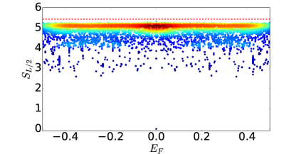
Figure 5: The bipartite entanglement entropy with equal partitions, $S_{L/2}$, shown for all the eigenstates of the Floquet unitary $U(T,0)$ with $\Delta_{0}=\omega_{D}=1$ for $L=24$ and $k=0$ (mod $\pi$). $E_{F}$ denotes the eigenvalue of $H_{F}$ and is defined in the interval $[-\pi/T,\pi/T)$. The horizontal dotted line indicates the average entanglement entropy, $S_{\mathrm{Page}}$, of random pure states. The density of states is indicated by a color map with warmer colors indicating higher density of states.

VI.3 PXP term

In this subsection, we consider the effect of adding a PXP Hamiltonian to $H_{3}$ so that

$$H_{\alpha} = H_{3}+\alpha H_{\rm PXP}$$ (48)

where $H_{3}$ and $H_{\rm PXP}$ are given by Eqs. 1 and LABEL:Hpxpdef respectively. Here $\alpha$ is a dimensionless parameter which determine the relative strength of the two terms in Eq. 48; in what follows, we shall restrict ourselves to $\alpha\ll 1$ and explore the effect of $H_{\rm PXP}$ in this perturbative regime starting from bubble initial states.

To understand the effect of $H_{\rm PXP}$ within the bubble manifold, we note $H_{\rm PXP}$ provides a dispersion to these bubbles which are strictly localized under the action of $H_{3}$. To justify this statement, let us first consider the effect of $H_{\rm PXP}$ on a bubble Fock state $|X_{1,j}\rangle$. It can be checked that

$$\sum_{j_{1}}\tilde{\sigma}^{x}_{j_{1}}|X_{1,j}\rangle = |\Phi_{2,j-1}\rangle+|\Phi_{2,j-3}\rangle$$

$$+|X_{2,j-1}\rangle+|X_{2,j+1}\rangle+|\psi^{\prime}\rangle$$

$$|\psi^{\prime}\rangle = |X_{1,j},X_{2,\ell}\rangle$$ (49)

where $\ell\neq j,j\pm 1,j\pm 2,j\pm 3$, $|\psi^{\prime}\rangle$ represent a state with one $X_{1}$ and one $X_{2}$ bubble whose centers are separated by at least three sites, and $|\Phi_{1(2)j}\rangle$ are given by Fourier transform of states defined Eq. 15. Note that $|\psi^{\prime}\rangle$ takes the system out of the subspace spanned by states $|X_{1,j}\rangle$, $|X_{2,j}\rangle$, $|\Phi_{1,j}\rangle$, and $|\Phi_{2,j}\rangle$. In what follows, we are going to ignore all such states. This step will be justified a posteriori while studying quantum dynamics induced by $H_{\alpha}$ starting from an initial state $|X_{1,j}\rangle$ in Sec. VII. Here we note that the effect of disregarding these additional state can be thought to lead to a decay rate, as per Fermi golden rule, leading to a loss of weight of the state $|X_{1,j}\rangle$ within the subspace. Such a decay rate clearly scales as $\alpha^{2}/\Delta E$ where $\Delta E$ denotes the energy difference of the eigenstates outside the subspace which have a finite matrix element with eigenstates within it. We have not been able to estimate $\Delta E$ in this work; we merely note that as long as $\Delta E\sim\mathrm{O}(\alpha)$ or larger, the decay rate will be small for small $\alpha$. We are going to address this issue while discussing dynamics induced by $H_{\alpha}$.

Ignoring the states $|\psi^{\prime}\rangle$, and noting $H_{3}|X_{1,j}\rangle=|X_{2,j}\rangle$, we find that a Fourier transform of Eq. 49 allows us to write

$$H_{\alpha}|X_{1,k}\rangle = \epsilon_{k}|X_{2,k}\rangle+c_{2k}|\Phi_{2,k}\rangle$$ (50)

$$\epsilon_{k} = (1+2\alpha\cos k),\quad c_{2k}=\alpha(e^{-ik}+e^{-3ik}),$$

where $|X_{1,k}\rangle=\sum_{j}\exp[ikj]|X_{1,j}\rangle$. An exactly similar consideration shows (ignoring the states outside the subspace)

$$H_{\alpha}|X_{2,k}\rangle = \epsilon_{k}|X_{1,k}\rangle+c_{1k}|\Phi_{1,k}\rangle$$

$$H_{\alpha}|\Phi_{1,k}\rangle = \beta_{k}|\Phi_{2,k}\rangle+c_{1k}^{\ast}|X_{2,k}\rangle,$$

$$H_{\alpha}|\Phi_{2,k}\rangle = \beta_{k}^{\ast}|\Phi_{1,k}\rangle+c_{2k}^{\ast}|X_{1,k}\rangle$$

$$\beta_{k} = (1+e^{ik}),\quad c_{1k}=\alpha(1+e^{-3ik})$$ (51)

Thus finding the eigenvalues of $H_{\alpha}$ in this subspace amounts to diagonalization of the $4\times 4$ matrix given by

$$\left(\begin{array}[]{cccc}0&\epsilon_{k}&c_{2k}&0\\ \epsilon_{k}&0&0&c_{1k}\\ c_{2k}^{\ast}&0&0&\beta_{k}\\ 0&c_{1k}^{\ast}&\beta_{k}^{\ast}&0\end{array}\right)$$ (56)

The four eigenvalues $E_{ik}$ for $i=1,2,3,4$ obtained by diagonalization of this matrix is shown in Fig. 6 We find that for $\alpha=0$, the action of $H_{3}$ correctly reproduces the flat band (corresponding to the subspace spanned by $|X_{1,k}\rangle$ and $|X_{2,k}\rangle$) and the dispersing band with $E_{K}=2\cos k/2$ (corresponding to the subspace spanned by $|\Phi_{1,k}\rangle$ and $|\Phi_{2,k}\rangle$). The states within each of these $2\times 2$ subspaces do not interact with those of the other subspace for $\alpha=0$ as seen from the top left panel of Fig. 6. Note the bands touch at $k=\pm 2\pi/3$.

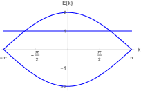
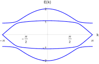
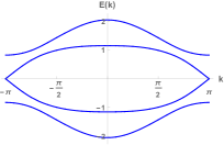
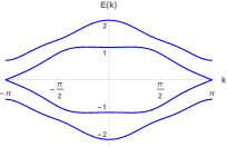
Figure 6: Plot of the energies $E_{ik}$ for $i=1,2,3,4$ of $H_{\alpha}$ within the $4\times 4$ subspace spanned by the bubble states $|X_{1(2),k}\rangle$ and $|\Phi_{1(2),k}\rangle$. The top left (right) panels correspond to $\alpha=0(0.05)$ and the bottom left (right) panels to $\alpha=0.1(0.2)$. Note that the hybridization spreads over larger region in the Brillouin zone with increasing $\alpha$.

On turning on $\alpha$, the band hybridizes due to interaction between states belonging to different $2\times 2$ subspaces. The hybridization occurs for any finite $\alpha$. However at small $\alpha$, it is significant only in the momentum width $\delta k=2\arccos(\alpha/2)$ around $k=\pm 2\pi/3$. Outside this range, the effect of hybridization is small. This can be clearly seen from top right and bottom panels of Fig. 6. Thus for small $\alpha\ll 1$, states in the $2\times 2$ subspace spanned by $|X_{1(2),k}\rangle$ do not interact with those in the subspace spanned by $|\phi_{1(2),k}\rangle$ for most momenta within the first Brillouin zone. We shall use the significance of this fact while discussing quench dynamics induced by $H_{\alpha}$ in Sec. VII.

VII Quench dynamics from some simple initial states

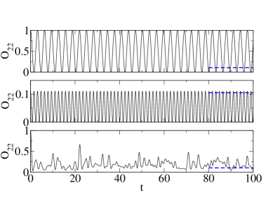
Figure 7: The evolution of a local correlation function as a function of time ($t$) for a system of $L=18$ for three different initial states (a bubble Fock state with a single $X_{1,j_{0}}$ at $j_{0}=3$ in the top panel, $|\Phi_{1,k=0}\rangle$ (Eq. 15) in the middle panel and $|\mathbb{Z}_{2}\rangle$ state in the bottom panel) quenched under $H_{3}$.

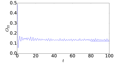
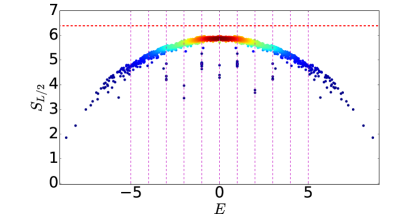
Figure 8: (Top panel) The evolution of a local correlation function as a function of time ($t$) for a system of $L=28$ for the initial state $(|\mathbb{Z}_{2}\rangle+|\bar{\mathbb{Z}}_{2}\rangle)/\sqrt{2}$. (Bottom panel) $S_{L/2}$ shown for all the eigenstates in the primary fragment with global quantum numbers $k=0,I=+1$ that contains the state $(|\mathbb{Z}_{2}\rangle+|\bar{\mathbb{Z}}_{2}\rangle)/\sqrt{2}$. The vertical dotted lines are given at integer values of $E$ in the bottom panel while the horizontal dotted line indicates the average entanglement entropy, $S_{\mathrm{Page}}$, of random pure states.

A dynamical consequence of Hilbert space fragmentation is the lack of thermalization starting from a class of simple initial states while other initial states thermalize (since the model is non-integrable). All the bubble-type Fock states defined in Sec. III provide examples of initial states that do not thermalize under a unitary evolution with $H_{3}$ and instead show perfectly coherent oscillations (except the inert Fock state since its an eigenstate of $H_{3}$). This phenomenon is easiest to see for a classical Fock state with a single $X_{1}/X_{2}$ unit (see Eq. 8) since such an initial state only has an overlap with two bubble-type eigenstates of $H_{3}$. The wavefunction at time $t$ starting from a state constituting a single $X_{1,j_{0}}$ bubble (denoted by $|X_{1,j_{0}}\rangle$ for clarity) is given by

$$|\psi_{1,j_{0}}(t)\rangle=\left(\cos t|X_{1,j_{0}}\rangle+\sin t|X_{2,j_{0}}\rangle\right)$$ (57)

where here and in the rest of this section, we have set $\hbar=1$. Thus local quantities like $\langle\sigma_{j}^{z}\rangle$ (where $j$ coincides with any of the three sites ($j_{0},j_{0}\pm 1$) within the bubble) show oscillations. For example, it is easy to see that when $j_{0}$ denotes the center site of the bubble

$$\langle\psi_{1j_{0}}(t)|\sigma_{j_{0}}^{z}|\psi_{1j_{0}}(t)\rangle = -\cos 2t$$

$$\langle\psi_{1j_{0}}(t)|\sigma_{j_{0}\pm 1}^{z}|\psi_{1j_{0})}(t)\rangle = \cos 2t$$ (58)

leading to an oscillation time period $T=\pi$. We note that a similar oscillation will also be seen for the global magnetization $M=\langle\sum_{j}\sigma_{j}^{z}\rangle$, albeit about an extensive constant expectation value, given by

$$M(t) = -\left((L-3)-\cos 2t\right).$$ (59)

where we have taken a chain of length $L$. In contrast, the staggered magnetization $M_{s}(t)=\langle\sum_{j}(-1)^{j}\sigma_{j}^{z}\rangle$ yields

$$M_{s}(t) = (-1)^{j_{0}+1}[3\cos 2t].$$ (60)

Thus $M_{s}$ exhibits $\pi$ periodic oscillation about zero. In addition, we shall also be computing the density-density correlation of the Rydberg atoms between two second-nearest neighbors. These can be written in terms of the spin operator as

$$O_{j_{1}2}=\langle n_{j_{1}}n_{j_{1}+2}\rangle=\frac{1}{4}\langle(1+\sigma_{j_{1}}^{z})(1+\sigma_{j_{1}+2}^{z})\rangle$$ (61)

For the bubble states, this correlator also leads to $\pi$ periodic oscillation

$$O_{j_{1}2}(t) = \delta_{j_{1}j_{0}-1}\cos^{2}(t)$$ (62)

This is shown numerically for a system of size $L=18$ in Fig. 7 (top panel) where we have plotted $O_{22}$ with $j_{0}=3$. The oscillation time period equals $T=\pi$ for more complicated bubble Fock states as well which follows from the “non-interacting” nature of $H_{3,\mathrm{bubble}}$ in Eq. 10. Another interpretation of the persistent oscillations is that there is an emergent dynamical symmetry that arises in the bubble sector since

$$[P_{\mathrm{bubble}}H_{3}P_{\mathrm{bubble}},\frac{\tau^{y}_{j_{b}}+i\tau^{z}_{j_{b}}}{2}]=\omega\left(\frac{\tau^{y}_{j_{b}}+i\tau^{z}_{j_{b}}}{2}\right)$$ (63)

where $P_{\mathrm{bubble}}$ is a projection operator to the bubble Fock space and $\omega=2$ given the form of $H_{3,\mathrm{bubble}}$ in Eq. 10. Thus, for a bubble Fock state, any local operator with a finite overlap with the any of the $\left(\frac{\tau^{y}_{j_{b}}+i\tau^{z}_{j_{b}}}{2}\right)$ operators will show persistent oscillations Medenjak2020 with a time period of $T=2\pi/\omega=\pi$.

On the other hand, if one starts with an initial state like $|\Phi_{1,k=0}\rangle$ (Eq. 15) which is a zero-momentum version of a non-bubble Fock state, we see that the corresponding oscillation time scale changes to $T=\pi/2$ because $\Delta E=4$ in this case (Fig. 7 (middle panel). Finally, there are simple initial states that are part of large non-bubble fragments which seem to thermalize close to the ETH-predicted steady state value. For example, the $|\mathbb{Z}_{2}\rangle$ state seems to be one such state. The temporal behavior of local correlators when the system is initialized in this state for $L=18$ (see Fig. 7 (bottom panel)) does not show coherent oscillations and instead gives a much more complicated dynamics.

To understand this better, we instead use the initial state $(|\mathbb{Z}_{2}\rangle+|\bar{\mathbb{Z}}_{2}\rangle)/\sqrt{2}$. Since this state belongs to the largest primary fragment of $k=0,I=+1$ sector for the system sizes $L=10,16,22,28\cdots$, the usage of momentum and spatial inversion symmetries allow us to study the dynamics for $L=28$ (Fig. 8 (top panel)). We see that in fact, unlike in the PXP model, the state appears to thermalize close to an infinite temperature ensemble (calculated using the states inside the primary fragment) when quenched under $H_{3}$, consistent with ETH (Fig. 8, top panel). In Fig. 8 (bottom panel), we plot $S_{L/2}$ for the eigenstates from the primary fragment at $k=0$, $I=+1$ that contains this particular state. A comparison with Fig. 3 (top left panel) immediately shows that while the entire symmetry sector contains several anomalous eigenstates, this particular primary fragment with the same global quantum numbers contains much fewer anomalous eigenstates. Moreover, these anomalous eigenstates have little overlap with $(|\mathbb{Z}_{2}\rangle+|\bar{\mathbb{Z}}_{2}\rangle)/\sqrt{2}$ which explains why the unitary dynamics under $H_{3}$ thermalizes this initial state.

The $H_{\Delta}$ interaction (Eq. VI.1) allows for the possibility of controlling the energy gaps between different eigenstates in the bubble-type fragments which can only be integers when $\Delta=0$. Using any bubble Fock state (except the inert state) and and following a similar analysis as shown earlier using $H_{\Delta,\mathrm{bubble}}$ in Eq. 30, we find that in the presence of $H_{\Delta}$, the local quantities such as $\langle\sigma_{j}^{z}\rangle$ again shows perfect coherent oscillations with time period $T=\pi/\sqrt{[1+(9\Delta^{2}/4)]}$. Thus, $T$ can be tuned by varying $\Delta$ as shown in Fig. 9 for a bubble-type Fock state with a single $X_{1,j}$ with $L=18$ centered around $j_{0}=3$ where we have plotted $O_{22}(t)$ as a function of time.

Next, we consider quenching dynamics of bubble Fock states (say with a single $X_{1,j}$ as shown in Fig. 10 for a chain of $L=18$) induced by $H_{\alpha}$ (Eq. 48). In this case, we find that the dynamics strongly depends of the value of $\alpha$. When $\alpha=0$, the Hilbert space fragmentation leads to perfect coherent oscillations with an infinite lifetime (Fig. 7 (a)). However, for any $\alpha\neq 0$, the presence of the PXP term in the Hamiltonian destroys the fragmentation. When $\alpha=0.01\ll 1$ (Fig. 10), we nonetheless see initial oscillations which decay with a timescale $t_{1}^{*}\sim 125$ followed by a revival. For $\alpha=0.02$ (Fig. 10), such revivals are evident first at $t_{1}^{*}\sim 60$ and then again at $t_{2}^{*}\sim 140$. For $\alpha=0.1$, a weak revival is also evident after $t_{1}^{*}\sim 12$ (Fig. 10). However, for $\alpha=0.5$, we see no oscillations and the state quickly relaxes to the ETH answer (Fig. 10).

To explain the revivals, we consider the limit $\alpha\ll 1$. As seen from Fig. 7, in this limit, the states within the $2\times 2$ subspace do not hybridize for most parts of the Brillouin zone. Using this fact and a straightforward analysis similar to the one carried earlier, we find

$$|\psi_{k}(t)\rangle\simeq\cos\epsilon_{k}t+\sin\epsilon_{k}t$$ (64)

provided we start from an initial state $|\psi_{k}(t=0)\rangle=|X_{1,k}\rangle$ (where $k$ denotes momentum). Thus the time evolution of $O_{(j_{0}-1)2}(t)$ starting from initial state given by a single bubble localized at $j=j_{0}$ is given by

$$O_{(j_{0}-1)2}(t) \simeq \frac{1}{2L}\sum_{\vec{k}}[1+\cos(2\epsilon_{k}t)]$$ (65)

$$= \frac{1}{2}[1+\cos(2t)J_{0}(2\alpha t)]$$

where we have used $\epsilon_{k}=1+2\alpha\cos k$ and $J_{0}(x)$ denotes zeroth order Bessel function. Thus for $t_{n}^{\ast}=x_{n}/(2\alpha)$, where $x_{n}$ denotes the position of $n^{\rm th}$ zero of $J_{0}(x)$, one expects the oscillations to vanish followed by a revival for $t>t_{n}^{\ast}$.

We note that for small $\alpha$, $t_{n}^{\ast}=t^{\ast}$ found from exact numerics; for example, for $\alpha=0.01$ (first panel of Fig. 10), $t^{\ast}=t_{1}^{\ast}\simeq 120$ (since $x_{1}=2.4$) while for $\alpha=0.02$ (second panel of Fig. 10), $t_{1}^{\ast}\simeq 60$ and $t_{2}^{\ast}\simeq 139$ (since $x_{2}\simeq 5.54$) matches the positions where oscillation vanishes. For a larger $\alpha=0.1$ (third panel of Fig. 10), while $t_{1}^{\ast}\simeq 12$ matches well with the numerics, the next revival at $t_{2}^{\ast}\simeq 28$ is harder to see because of the decay of the oscillations. For still larger $\alpha=0.5$ (fourth panel of Fig. 10), the local observable rapidly attains the value. Moreover for $t\ll\alpha^{-1}$, the oscillations have $\pi$ periodicity as expected from Eq. 65.

While these features are reproduced by this calculation (revival and initial period of oscillations), there are several aspects of the dynamics which are not captured by this rather simplistic approach. For example, we find that $O_{(j_{0}-1)2}(t)$ almost touches zero at several times during the oscillation which can not be explained by Eq. 65 even when we take into account the possibility of its modification by a simple exponential decay factor which may stem from the loss of weight of the initial state from the $4\times 4$ subspace. Moreover, Eq. 65 predicts a value $O_{(j_{0}-1)2}(t_{n}^{\ast})=1/2$ for any $t_{n}^{\ast}$; instead exact numerics yields a value close to zero. We do not have an analytic explanation of these features of $O_{(j_{0}-1)2}(t)$.

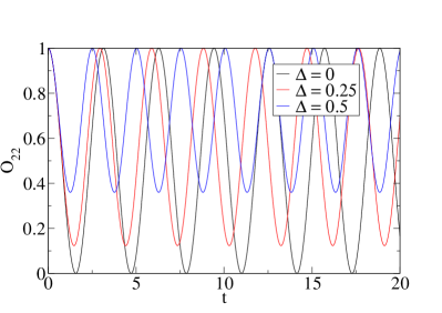
Figure 9: Unitary dynamics starting from an initial bubble Fock state with a single $X_{1,j_{0}}$ with $j_{0}=3$ quenched under $H_{\Delta}$ for three different values of $\Delta$ for a chain of length $L=18$.

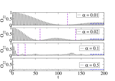
Figure 10: Unitary dynamics starting from an initial bubble Fock state with a single $X_{1,j}$ quenched under $H_{3}+\alpha H_{\mathrm{PXP}}$ for four different values of $\alpha$ for a chain length of $L=18$. The vertical lines in the top three panels are drawn at $t_{n}^{\ast}=x_{n}/(2\alpha)$ where $x_{n}$ denote the zeroes of the Bessel function $J_{0}(x)$ as a guide to the eye.

VIII Mapping to a lattice gauge theory

In this section, we show how to exactly map the $H_{3}$ model (Eq. 1) to a Hamiltonian formulation of a $U(1)$ lattice gauge theory coupled to fermionic matter in one dimension and interpret some of the results of the previous sections in the language of this gauge theory. Such a mapping was already implemented in Ref. SuracePRX, for the PXP model and we generalize the same to the $H_{3}$ model here.

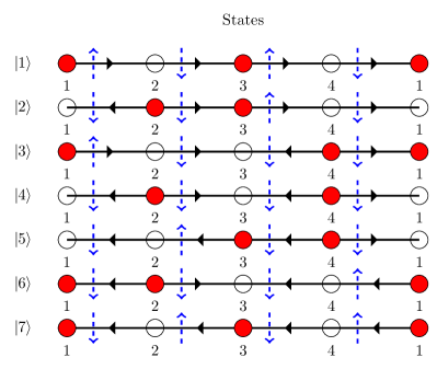
Figure 11: One-to-one correspondence shown between the gauge-invariant states that obey Eq. 67 and the Fock states in the constrained Hilbert space where no two adjacent $S^{z}$ can be $\uparrow\uparrow$ simultaneously for a chain length of $L=4$ with periodic boundary conditions. The fermionic matter resides on the sites denoted by circles (where a filled (unfilled) circle represents presence (absence) of fermions) while the electric fluxes live on the bonds between these circles (denoted by horizontal arrows). The corresponding $S^{z}=\uparrow,\downarrow$ spins are shown as dotted blue arrows on the dual sites.

The mapping between the Fock states in the constrained Hilbert space and the gauge degrees of freedom is illustrated for a $L=4$ system in Fig. 11. The gauge degrees live on the links connecting two neighboring sites $i$ and $i+1$ of a one-dimensional lattice while the fermionic matter fields live on the sites. The original spins can be thought to reside on the sites of the dual lattice. Both the problems are assumed to have periodic boundary conditions. The gauge degrees are quantum spin $S=1/2$ operators with the electric flux $E_{i,i+1}=S^{z}_{i,i+1}$ with a $U(1)$ quantum link, $U_{i,i+1}=S^{+}_{i,i+1}$ being a raising operator for it (see Ref. QLM, for the formulation of such quantum link models and their spin-$S$ representation). The electric flux on the links are related to the original spins on the corresponding dual sites by the relation

$$E_{i,i+1}=(1/2)\eta_{i}\sigma^{z}_{d(i,i+1)}$$ (66)

where, according to our sign convention (e.g., see Fig. 11), $\eta_{i}=+1$ ($-1$) if $i$ is an odd (even) site and $\sigma^{z}_{d(i,i+1)}=\pm 1$ refers to the original spin residing on the dual site between the link that connects $i$ and $i+1$. The fermionic creation operator for the matter field at site $i$ is denoted by $\psi_{i}^{\dagger}$ and the corresponding number operator equals $n_{i}=\psi_{i}^{\dagger}\psi_{i}$ (whose eigenvalues equal $0$ or $1$). The matter field at site $i$ is “slaved” to the corresponding electric fluxes on links with $i$ and is defined by the following Gauss law:

$$E_{i,i+1}-E_{i-1,i}=\psi_{i}^{\dagger}\psi_{i}+\left(\frac{(-1)^{i}-1}{2}\right).$$ (67)

The Gauss law automatically implements the correct kinematic constraints on the Hilbert space as can be verified by constructing all the gauge-invariant states (as shown in Fig. 11) for $L=4$. Fig. 11 also shows the original spins on the dual sites for each of these states, showing the one-to-one correspondence between gauge-invariant states and the Fock states of the original spins. Thus, the number of gauge-invariant states on a lattice with $L$ sites with periodic boundary conditions also equals $F_{L-1}+F_{L+1}$ where $F_{j}$ is the $j$th Fibonacci number. Ref. SuracePRX, showed that $H_{\mathrm{PXP}}$ (Eq. LABEL:Hpxpdef can then be written as

$$H_{\mathrm{PXP}}=\sum_{i=1}^{L}(\psi_{i}^{\dagger}U_{i,i+1}\psi_{i+1}+\mathrm{H.c.})$$ (68)

which represents a gauge theory with a minimal coupling between the gauge and matter fields.

Using the exact mapping between the original spins and the gauge degrees of freedom, the $H_{3}$ interaction (Eq. 1) can also be written as

$$H_{3} = \sum_{i=1}^{L}(\psi_{i}^{\dagger}\Box_{i,i+3}\psi_{i+3}\Gamma_{i+1}\Gamma_{i+2}+\mathrm{H.c.})$$

$$\Box_{i,i+3} = U_{i,i+1}U_{i+1,i+2}U_{i+2,i+3}$$ (69)

where $\Gamma_{j}=n_{j}$ for odd $j$ and $\Gamma_{j}=(1-n_{j})$ for even $j$. That Eq. 69 defines another $U(1)$ lattice gauge theory may be verified by checking that $[H_{3},G_{i}]=0$ for all $i$ where $G_{i}=E_{i,i+1}-E_{i-1,i}-\psi_{i}^{\dagger}\psi_{i}-\left(\frac{(-1)^{i}-1}{2}\right)$ are the generators of the $U(1)$ gauge symmetry. Furthermore, $E_{i,i+1}-E_{i-1,i}=Q_{i}$ where $Q_{i}$ defines the local charge on site $i$ and can equal either $\pm 1$ or $0$.

It is useful to consider the charge configurations associated to the allowed Fock states in the Hilbert space. Firstly, the reference (or the inert state) has an alternating configuration of $Q_{i}=+1$ ($Q_{i}=-1$) charges on even (odd) $i$. Any other valid charge configuration can be obtained from this reference charge configuration by selecting pairs of $+1$ and $-1$ charges on arbitrary sites and annihilating them to form neutral charges $0$ on the same sites. The lattice gauge theory defined by $H_{3}$ (Eq. 69) induces the following charge dynamics

$$H_{3} = \sum_{i\in\mathrm{even}}(|+1_{i}0_{i+1}0_{i+2}-1_{i+3}\rangle\langle 0_{i}0_{i+1}0_{i+2}0_{i+3}|$$ (70)

$$+ \mathrm{H.c.})$$

$$+ \sum_{i\in\mathrm{odd}}(|-1_{i}0_{i+1}0_{i+2}+1_{i+3}\rangle\langle 0_{i}0_{i+1}0_{i+2}0_{i+3}|$$

$$+ \mathrm{H.c.}).$$

Unlike earlier models PaiPN2019 ; KhemaniN2019 ; Khemani2020 ; SalaRVKP2020 ; MoudgalyaPNRB2019 of Hilbert space fragmentation where both total charge and dipole-moment were simultaneously conserved, this $U(1)$ gauge theory only conserves the total charge but not the dipole moment. This can be easily seen by taking a charge-neutral configuration with $Q_{i}=0$ on all sites and then placing a $Q_{2j}=+1$ and $Q_{2j+1}=-1$ on two adjacent sites to create a dipole of length $l=1$. The charge dynamics induced by $H_{3}$ (Eq. 70) then creates longer dipoles leading to a non conservation of the net dipole moment, as we illustrate below:

$$\cdots 00\boxed{+1}\boxed{-1}00000000\rightarrow\cdots 00\boxed{+1}\boxed{-1}00\boxed{+1}00\boxed{-1}00\cdots\rightarrow\cdots 00\boxed{+1}000000\boxed{-1}00\cdots.$$ (71)

The bubble Fock states defined in Sec. III have a simple interpretation in this language. Let us start with the reference configuration and select any four consecutive sites and make the charges on these four sites to be zero. This charge configuration is connected to only one other charge configuration through the dynamics induced by $H_{3}$ (Eq. 70):

$$\cdots -1 +1-1\boxed{0_{j}000}+1-1+1\cdots$$

$$\cdots -1 +1-1\boxed{+1_{j}00-1}+1-1+1\cdots$$ (72)

and all the charges outside $\boxed{Q_{j}00Q_{j+3}}$ are completely frozen. These are the one bubble Fock states that we defined earlier. On the other hand, the charge dynamics induced by $H_{\mathrm{PXP}}$ (Eq. 68

$$H_{\mathrm{PXP}} = \sum_{i\in\mathrm{even}}(|+1_{i}-1_{i+1}\rangle\langle 0_{i}0_{i+1}|+\mathrm{H.c.})$$ (73)

$$+ \sum_{i\in\mathrm{odd}}(|-1_{i}+1_{i+1}\rangle\langle 0_{i}0_{i+1}|+\mathrm{H.c.}),$$

does not keep the charges outside $\boxed{Q_{j}00Q_{j+3}}$ as frozen since there are several adjacent pairs of $\pm 1\mp 1$ charges provided by the background of the reference configuration.

To build two bubble Fock states, we simply need to satisfy the constraint that these units $\boxed{Q_{j}00Q_{j+3}}$ and $\boxed{Q_{\ell}00Q_{\ell+3}}$ when inserted in the reference configuration should have at least one site separating them. The minimum case with a single site separating the two units is shown below:

$$\cdots +1 -1\boxed{0_{j}000}+1\boxed{0_{\ell}000}-1+1\cdots$$

$$\cdots +1 -1\boxed{+1_{j}00-1}+1\boxed{0_{\ell}000}-1+1\cdots$$

$$\cdots +1 -1\boxed{0_{j}000}+1\boxed{-1_{\ell}00+1}-1+1\cdots$$

$$\cdots +1 -1\boxed{+1_{j}00-1}+1\boxed{-1_{\ell}00+1}-1+1\cdots$$

where the charges outside the two units $\boxed{Q_{j,\ell}00Q_{j+3,\ell+3}}$ are frozen. To form an $n$ bubble Fock state, we simply need to insert $n$ such $\boxed{Q_{j}00Q_{j+3}}$ units, where $Q_{j}=-Q_{j+3}$ and $Q_{j}$ can be either $0$ or $+1$ ($-1$) if $j$ is even (odd), and these units are separated by at least one site in between them with the rest of the charges following the charge configuration of the reference configuration. The bubble eigenstates of $H_{3}$ are then formed using $(|\boxed{\pm 100\mp 1}\rangle\pm|\boxed{0000}\rangle)/\sqrt{2}$ units and the frozen charges as before.

It is interesting to point out that the gauge-invariant states corresponding to any of the bubble Fock states show a restricted mobility of the elementary charged excitations under the dynamics induced by $H_{3}$ (Eq. 70). This is because while all charges outside the $\boxed{Q_{j}00Q_{j+3}}$ units are completely immobile, the charges inside the units can fluctuate between $\boxed{\pm 100\mp 1}$ and $\boxed{0000}$ showing that only dipoles of length three (in terms of lattice spacing) are mobile. Thus, the bubble states in the gauge theory show an emergent fractonic behavior since the charges have a highly reduced mobility.

The non-bubble eigenstates with dispersing quasiparticles as discussed in Sec. IV also have a simple interpretation in terms of the charge configurations. For this, we start with the non-bubble Fock state where a unit of six consecutive sites have zero charge, $\boxed{0_{j}00000}$, while the rest of the sites follow the charge configuration of the reference state. The action of $H_{3}$ (Eq. 70) then leads to an effective hopping of this six-charge unit either in the forward or backward direction through intermediate charge units $\boxed{\pm 1_{j}0000\mp 1}$ that also move forward or backward in the same manner. This is shown explicitly in Eq. 75 for the forward motion of these units.

$$\cdots -1 +1-1\boxed{0_{j}00000}+1-1+1\cdots\leftrightarrows\cdots-1+1-1\boxed{+1_{j}00-100}+1-1+1\cdots\leftrightarrows$$

$$\cdots -1 +1-1+1\boxed{0_{j+1}00000}-1+1\cdots\leftrightarrows\cdots-1+1-1+1\boxed{-1_{j+1}00+100}-1+1\cdots$$ (75)

These charge configurations provide the exact analog of the Fock states in Eq. 14 and the rest of the steps can be traced similarly. Looking at the charge configurations in Eq. 75, we see that length three dipoles attached to two neutral charges (i.e., $\boxed{\pm 100\mp 1}00$ or alternatively $00\boxed{\pm 100\mp 1}$) are the effective mobile units here, again suggesting a connection to fractons. Whether the restricted mobility of longer, more complicated charge-neutral units give rise to (some of) the other anomalous states is an interesting open question.

IX Conclusions and outlook

In this work, we have considered a minimal model for Hilbert space fragmentation on a one-dimensional ring defined in terms of $S=1/2$ quantum spins with three-spin interactions between them along with the hard constraint that no two adjacent spins can have $S^{z}=\uparrow$ together. Like the prototypical model PXP model, the many-body spectrum of this model is also reflection-symmetric around $E=0$ and admits an exponentially large number (in system size) of exact mid-spectrum zero modes due to an index theorem. Additionally, the spectrum has exact degeneracies at other integer eigenvalues (after a suitable choice of Hamiltonian normalization) for arbitrary chain lengths.

In spite of the non-integrable nature of this model, a class of its high-energy eigenstates can be shown to violate the eigenstate thermalization hypothesis in the thermodynamic limit. This is due to a combination of the kinematic constraints and the nature of interactions which causes the Hilbert space to fracture into disconnected fragments that are closed under the action of the Hamiltonian. These fragments cannot be distinguished by their global quantum numbers alone and the largest such fragment, though exponentially large in the system size, still occupies a vanishingly small fraction of the total Hilbert space in the thermodynamic limit. This fragmentation allows for closed-form expressions for many of the high-energy eigenstates in terms of quasiparticles.

The simplest class of such eigenstates, the so-called bubble eigenstates, are composed of strictly localized quasiparticles and have a natural representation in real space. These eigenstates emerge from fragments composed exclusively of bubble Fock states with the smallest such fragment being $1\times 1$ and the largest being $2^{n_{0}}\times 2^{n_{0}}$ where $n_{0}\sim L/5$ with $L$ being the chain length. All the bubble eigenstates have integer eigenvalues (including zero) and follow strict area law for entanglement entropy. A lower bound on the number of such states demonstrates that their number grows exponentially with system size for integer energies from zero to $\pm\mathrm{O}(\sqrt{L})$ when $L\gg 1$.

Furthermore, we have been able to write closed-form expressions for a class of anomalous high-energy eigenstates that belong to fragments generated from non-bubble Fock states in this model. These eigenstates are all expressed in terms of mobile quasiparticles and thus have a natural representation in momentum space. The simplest of these belong to $2\times 2$ fragments where the basis states are generated using certain non-bubble Fock states and their translations. These eigenstates have eigenvalues that lead to two dispersive bands at high energies that consist of irrational eigenvalues in general when $L\gg 1$.

We have pointed out a novel secondary fragmentation mechanism in this model whereby a class of eigenstates of non-bubble type fragments can be analytically calculated even when the dimension of the fragment grows rapidly with system size. This is because certain linear combinations of a fixed number of basis states in momentum space (whose number does not scale with the system size) leads to formation of a smaller secondary fragment of a fixed dimension inside the large primary fragment, with the states inside the secondary fragment being disconnected from the rest of the Hilbert space under the action of the Hamiltonian. We show the existence of two anomalous eigenstates (with energies $E=\pm 1$) in the sector with zero momentum and spatial inversion symmetry and two flat bands (with energies $E=\pm 1$) in momentum space via this mechanism.

At this point, it is useful to again stress on some of the key differences compared to other models of Hilbert space fragmentation in the literature. While previous models had two simultaneous $U(1)$ conservation laws (with these being “charge” and “dipole” conservations in most cases), this model does not have such simultaneous conservations. Rather, the fragmentation is produced due to an interplay of interactions and the constrained nature of the Hilbert space; conservation laws emerge for specific sectors as discussed in Sec. VIII. While previous models had an exponentially large number of “inert” states which formed $1\times 1$ fragments on their own due to the global charge and dipole conservation laws, this model has only one such inert state due to the absence of dipole conservation (Sec. VIII). Lastly, the secondary fragmentation mechanism for this model that leads to some anomalous eigenstates even in large primary fragments with most states being typical has not been pointed out in earlier studies to the best of our knowledge.

We considered the effects of adding two different non-commuting interactions to the minimal model. Both the perturbed models still continue to have an $E\rightarrow-E$ symmetry and an exponentially large number (with system size) of zero modes in their many-body spectra. The perturbation with a staggered magnetic field term preserves Hilbert space fragmentation and gives the same number of zero modes for any non-zero and finite value of the field based on exact diagonalization results on small chains ($L\leq 20$). We were able to analytically understand a class of these zero modes and their eigenstates. We also defined a Floquet version with a periodically driven staggered magnetic field and showed that the Floquet unitary continues to have a large class of eigenstates with area law entanglement. The Floquet version has the added feature that all initial bubble Fock states show exact stroboscopic freezing at an infinite number of special drive frequencies even in the thermodynamic limit. Another perturbation with the PXP term is more complicated since it immediately destroys the Hilbert space fragmentation of the unperturbed model. However, an approximate treatment was still possible for certain initial states when the perturbation can be considered to be small.

Quench dynamics starting from some simple initial states were also discussed. While bubble Fock states showed coherent oscillations in local observables such as $O_{22}$, the frequency of which could be tuned by adding a suitable staggered magnetic field, some other states like the Néel state rapidly thermalized (unlike in the PXP model). Quenching with the perturbed model with a PXP term showed qualitative distinctions between the small perturbation case and otherwise. In the small perturbation limit, we found $O_{22}$ to exhibit oscillations with revivals enclosed within a decaying envelope; the position of the revivals and the time period of the short-time oscillations was understood using a simple, analytically tractable, model. However, other details of the dynamics such as the decay rate could not be understood analytically. With increasing strength of the PXP term, the oscillatory behavior is lost and we found a rapid decay to the ETH predicted thermal value.

We showed how to map this model to an exact $U(1)$ quantum link model in its $S=1/2$ representation interacting with dynamical fermions. The Gauss law in the gauge theory automatically enforced the constraints in the Hilbert space. We interpreted some of the anomalous eigenstates in this language and also showed that the charged degrees of freedom have reduced mobility for these states with only certain charge-neutral objects being mobile, a tell-tale signature of fractons.

Several open issues emerge from our study. Exact diagonalization results on small chains ($L\leq 20$) already show that while the bubble eigenstates exhaust the count of integer eigenstates close to $|E|\sim n_{0}$ with $n_{0}\sim L/5$, there are many more non-bubble eigenstates that are integer-valued in the vicinity of $E=0$ with their numbers rapidly increasing with system size. While the bubble eigenstates follow strict area law scaling of entanglement entropy and we have shown a few examples of non-bubble integer eigenstates that are anomalous, we believe that the majority of these non-bubble integer eigenstates in the neighborhood of $E=0$ (with the extend of $|E|\sim\mathrm{O}(\sqrt{L})$ to be precise) may have volume law scaling of entanglement entropy when $L\gg 1$. It will be useful to address this issue both theoretically and numerically using techniques similar to Ref. Karle, . While we have a complete understanding of the bubble eigenstates in this minimal model, it will be useful to see if a deeper understanding can be obtained for the non-bubble anomalous eigenstates, especially those generated by secondary fragmentation. After mapping this model to a $U(1)$ lattice gauge theory, we see that it only has charge conservation unlike earlier fractonic gauge theories, where some higher moment is also conserved. However, different charge-neutral units with reduced mobilities arise when focusing on a class of the anomalous states. Addressing this emergent fractonic physics in this gauge theory is left for future works. It seems possible to generalizing this model to two dimensions in multiple ways and it will be interesting to see whether the higher-dimensional versions violate the eigenstate thermalization hypothesis as well.

Lastly, it is likely that the Hilbert space fragmentation mechanism and anomalous dynamics from certain initial states that we have discussed may be realized using a Floquet setup. Refs. dyn1, ; dyn5, showed that a certain periodic drive protocol wherein a time-periodic magnetic field is applied to the PXP model results in a Floquet Hamiltonian with both PXP and non-PXP type terms with the $H_{3}$ interaction being the leading non-PXP interaction with the subsequent sub-dominant terms becoming more long-ranged (e.g., an $H_{5}$ interaction involving five-spin terms, an $H_{7}$ interaction involving seven-spin terms, and so on). Ref. dyn5, showed that tuning the drive frequency alone, it is possible to make the coefficient of the PXP term go to zero in the Floquet Hamiltonian which leads to freezing of the reference state with all $S^{z}=\downarrow$. At these drive frequencies, the Floquet Hamiltonian is also fragmented since the reference state forms a $1\times 1$ fragment of its own. To see coherent oscillations from bubble-type Fock states, a Floquet protocol is needed where the coefficients of both the PXP and the $H_{5}$ interactions can be simultaneously tuned to zero. Since the longer-ranged terms like $H_{7}$ etc annihilate any bubble-type Fock states with distant bubbles, these coefficients need not be fine-tuned.

- (1) J. M. Deutsch, Phys. Rev. A 43, 2046 (1991).
- (2) M. Srednicki, Phys. Rev. E 50, 888 (1994).
- (3) M. Rigol, V. Dunjko, and M. Olshanii, Nature 452, 854 (2008).
- (4) A. Polkovnikov, K. Sengupta, A. Silva, and M. Vengalattore, Rev. Mod. Phys. 83, 863 (2011).
- (5) L. D’Alessio, Y. Kafri, A. Polkovnikov, and M. Rigol, Advances in Physics 65, 239 (2016).
- (6) P. Reimann, New Journal of Physics 17, 055025 (2015).
- (7) C. Gogolin and J. Eisert, Rep. Prog. Phys. 79, 056001 (2016).
- (8) L. Vidmar and M. Rigol, Journal of Statistical Mechanics: Theory and Experiment 2016, 064007 (2016).
- (9) A. Pal and D. A. Huse, Phys. Rev. B 82, 174411 (2010).
- (10) R. Nandkishore and D. A. Huse, Annu. Rev. Condens. Matter Phys. 6, 15 (2015).
- (11) H. Bernien, S. Schwartz, A. Keesling, H. Levine, A. Omran, H. Pichler, S. Choi, A. S. Zibrov, M. Endres, M. Greiner, V. Vuletić, and M. D. Lukin, Nature 551, 579 (2017).
- (12) C. J. Turner, A. A. Michailidis, D. A. Abanin, M. Serbyn, and Z. Papić, Nat. Phys. 14, 745 (2018).
- (13) C. J. Turner, A. A. Michailidis, D. A. Abanin, M. Serbyn, and Z. Papić, Phys. Rev. B 98, 155134 (2018).
- (14) S. Sachdev, K. Sengupta, and S. M. Girvin, Phys. Rev. B 66, 075128 (2002).
- (15) P. Fendley, K. Sengupta, and S. Sachdev, Phys. Rev. B 69, 075106 (2004).
- (16) I. Lesanovsky and H. Katsura, Phys. Rev. A 86, 041601(R) (2012).
- (17) T. Iadecola, M. Schecter, and S. Xu, Phys. Rev. B 100, 184312 (2019).
- (18) N. Shiraishi, J. Stat. Mech. (2019) 083103.
- (19) S. Moudgalya, N. Regnault, and B. A. Bernevig, Phys. Rev. B 98, 235156 (2018).
- (20) S. Moudgalya, S. Rachel, B. A. Bernevig, and N. Regnault, Phys. Rev. B 98, 235155 (2018).
- (21) D. K. Mark, C. -J. Lin, and O. I. Motrunich, Phys. Rev. B 101, 195131 (2020).
- (22) S. Moudgalya, E. O’ Brien, B. A. Bernevig, P. Fendley, and N. Regnault, Phys. Rev. B 102, 085120 (2020).
- (23) S. Moudgalya, B. A. Bernevig, and N. Regnault, Phys. Rev. B 102, 195150 (2020).
- (24) B. Nachtergaele, S. Warzel, and A. Young, J. Phys. A: Math. Theor. 54 01LT01 (2021).
- (25) O. Vafek, N. Regnault, and B. A. Bernevig, SciPost Phys. 3, 043 (2017).
- (26) T. Iadecola and M. Žnidarič, Phys. Rev. Lett. 123, 036403 (2019).
- (27) D. K. Mark and O. I. Motrunich, Phys. Rev. B 102, 075132 (2020).
- (28) S. Moudgalya, N. Regnault, and B. A. Bernevig, Phys. Rev. B 102, 085140 (2020).
- (29) M. Schecter and T. Iadecola, Phys. Rev. Lett. 123, 147201 (2019).
- (30) B. Mukherjee, S. Nandy, A. Sen, D. Sen, and K. Sengupta, Phys. Rev. B 101, 245107 (2020).
- (31) S. Sugiura, T. Kuwahara, and K. Saito, Phys. Rev. Research 3, L012010 (2021).
- (32) S. Pai and M. Pretko, Phys. Rev. Lett. 123, 136401 (2019).
- (33) B. Mukherjee, A. Sen, D. Sen, and K. Sengupta, Phys. Rev. B 102, 014301 (2020).
- (34) B. Mukherjee, A. Sen, D. Sen, and K. Sengupta, Phys. Rev. B 102, 075123 (2020).
- (35) H. Zhao, J. Vovrosh, F. Mintert, and J. Knolle, Phys. Rev. Lett. 124, 160604 (2020).
- (36) K. Mizuta, K. Takasan, and N. Kawakami, Phys. Rev. Research 2, 033284 (2020).
- (37) A. A. Michailidis, C. J. Turner, Z. Papić, D. A. Abanin, and M. Serbyn, Phys. Rev. Research 2, 022065 (2020).
- (38) C. -J. Lin, V. Calvera, and T. H. Hsieh, Phys. Rev. B 101, 220304(R) (2020).
- (39) K. Lee, R. Melendrez, A. Pal, and H. J. Changlani, Phys. Rev. B 101, 241111(R) (2020).
- (40) P. A. McClarty, M. Haque, A. Sen, and J. Richter, Phys. Rev. B 102, 224303 (2020).
- (41) D. Banerjee and A. Sen, Phys. Rev. Lett. 126, 220601 (2021).
- (42) M. Serbyn, D. A. Abanin, Z. Papić, Nat. Phys. 17, 675(2021).
- (43) C. Chamon, Phys. Rev. Lett. 94, 040402 (2005).
- (44) J. Haah, Phys. Rev. A 83, 042330 (2011).
- (45) S. Vijay, J. Haah, and L. Fu, Phys. Rev. B 94, 235157 (2016).
- (46) M. Pretko, Phys. Rev. B 95, 115139 (2017).
- (47) S. Pai, M. Pretko, and R. M. Nandkishore, Phys. Rev. X 9, 021003 (2019).
- (48) V. Khemani, M. Hermele and R. Nandkishore, Phys. Rev. B 101, 174204 (2020).
- (49) V. Khemani, M. Hermele, and R. Nandkishore, Phys. Rev. B 101, 174204 (2020).
- (50) P. Sala, T. Rakovszky, R. Verresen, M. Knap, and F. Pollmann, Phys. Rev. X 10, 011047 (2020).
- (51) S. Moudgalya, A. Prem, R. Nandkishore, N. Regnault, and B. A. Bernevig, arXiv:1910.14048.
- (52) Z-C. Yang, F. Liu, A. V. Gorshkov, and T. Iadecola, Phys. Rev. Lett. 124, 207602 (2020).
- (53) G. De Tomasi, D. Hetterich, P. Sala, and F. Pollmann, Phys. Rev. B 100, 214313 (2019).
- (54) C. M. Langlett and S. Xu, Phys. Rev. B 103, L220304 (2021).
- (55) B. Mukherjee, Z. Cai, and W. V. Liu, Phys. Rev. Research 3, 033201 (2021).
- (56) D. Hahn, P. A. McClarty, and D. J. Luitz, arXiv: 2104.00692.
- (57) K. Lee, A. Pal, and H. J. Changlani, Phys. Rev. B 103, 235133 (2021).
- (58) S. Scherg, T. Kohlert, P. Sala, F. Pollmann, Bharath H. M., I. Bloch, and M. Aidelsburger, Nat. Communications 12, 4490 (2021).
- (59) M. Schecter and T. Iadecola, Phys. Rev. B 98, 035139 (2018).
- (60) A. Lazarides, A. Das, and R. Moessner, Phys. Rev. E 90, 012110 (2014).
- (61) P. Ponte, A. Chandran, Z. Papić, and D. A. Abanin, Ann. Phys. 353, 196 (2015).
- (62) L. D’. Alessio and M. Rigol, Phys. Rev. X 4, 041048 (2014).
- (63) A. Soori and D. Sen, Phys. Rev. B 82, 115432 (2010).
- (64) T. Bilitewski and N. Cooper, Phys. Rev A 91, 063611 (2015).
- (65) A. Sen, D. Sen, and K. Sengupta, J. Phys. Cond. Mat. 33 443003 (2021).
- (66) D. N. Page, Phys. Rev. Lett. 71, 1291 (1993).
- (67) A. Das, Phys. Rev. B 82, 172402 (2010)
- (68) S. Mondal, D. Pekker, and K. Sengupta, Europhys. Lett. 100, 60007 (2012).
- (69) M. Medenjak, B. Buc̆a, and D. Jaksch, Phys. Rev. B 102, 041117 (R) (2020).
- (70) F. M. Surace, P. P. Mazza, G. Giudici, A. Lerose, A. Gambassi, and M. Dalmonte, Phys. Rev. X 10, 021041 (2020).
- (71) S. Chandrasekharan and U.-J. Wiese, Nucl. Phys. B492, 455 (1997).
- (72) V. Karle, M. Serbyn, and A. A. Michailidis, Phys. Rev. Lett. 127, 060602 (2021).