On Stochastic Partial Differential Equations and their applications to Derivative Pricing through a conditional Feynman-Kac formula

Abstract.

In a multi-dimensional diffusion framework, the price of a financial derivative can be expressed as an iterated conditional expectation, where the inner conditional expectation conditions on the future of an auxiliary process that enters into the dynamics for the spot. Inspired by results from non-linear filtering theory, we show that this inner conditional expectation solves a backward SPDE (a so-called ‘conditional Feynman-Kac formula’), thereby establishing a connection between SPDE and derivative pricing theory. Unlike situations considered previously in the literature, the problem at hand requires conditioning on a backward filtration generated by the noise of the auxiliary process and enlarged by its terminal value, leading us to search for a backward Brownian motion in this filtration. This adds an additional source of irregularity to the associated SPDE which must be tackled with new techniques. Moreover, through the conditional Feynman-Kac formula, we establish an alternative class of so-called mixed Monte-Carlo PDE numerical methods for pricing financial derivatives. Finally, we provide a simple demonstration of this method by pricing a European put option.

1. Introduction

The purpose of this article is to demonstrate that certain types of Stochastic Partial Differential Equations (SPDEs) naturally arise in derivative pricing. Briefly, let $X$, $V$, and $\mathfrak{r}$ be the asset price process, an auxiliary process (often stochastic variance/volatility), and deterministic interest rate respectively, see Section 2 for their definitions. One can express the price at time $t$ of a derivative $H$ with payoff $\varphi$ at time $T$ as an iterated conditional expectation under a chosen risk-neutral measure in the following fashion:

$$H_{t} =e^{-\int_{t}^{T}\mathfrak{r}_{s}\mathrm{d}s}\,\mathbb{E}\big{[}u(t,X_{t})|X_{t},V_{t}\big{]},$$

where

$$u(t,x):=\mathbb{E}[\varphi(X_{T})|X_{t}=x,\mathcal{G}_{t,T}].$$

Here $\mathcal{G}_{t,T}$ is a suitable $\sigma$-algebra which essentially corresponds to the future of the auxiliary process $V$ over $[t,T]$. Thus $u(t,x)$ is a random field which is $\mathcal{G}_{t,T}$ measurable for each fixed $x$. If we denote by $V_{[t,T]}$ the trajectory of $V$ over $[t,T]$, then at least informally, one can think of $u(t,x)$ as a functional of $V_{[t,T]}$, namely $u(t,x)\equiv u(t,x,V_{[t,T]})$.

We will prove that $u(t,x)$ solves a backward linear SPDE, similar to the usual Feynman-Kac formula from the deterministic PDE scenario. Such a relationship is known in the literature as a conditional Feynman-Kac formula, and many versions of these formulas have been studied in the literature, albeit in the context of non-linear filtering theory, see [9, 5, 10, 8, 6]. Recently, these results have been exploited in the context of generative modelling see [4]. Naturally, the existence and regularity properties of these types of SPDEs that arise through the conditional Feynman-Kac formulas are of great importance.

An important application of the conditional Feynman-Kac formula is in the development of a mixed Monte-Carlo PDE method for pricing financial derivatives. Indeed, we see from the first paragraph that the time $0$ price of a European derivative is given by

$$H_{0}=e^{-\int_{0}^{T}\mathfrak{r}_{r}\mathrm{d}r}\mathbb{E}[u(0,x)].$$

Through our conditional Feynman-Kac formula, $u(t,x)$ solves a backward SPDE. Thus the basic idea for the mixed Monte-Carlo PDE method is to simulate the price $H_{0}$ by simply numerically solving the backward SPDE repeatedly to obtain many i.i.d. copies of $u(0,x)$, and then averaging over them.

In this article we will prove a version of the conditional Feynman-Kac formula corresponding to the derivative pricing problem outlined above, and moreover we will study the existence and regularity of the associated SPDE. Unfortunately, the succinct martingale arguments typically used in modern proofs for Feynman-Kac formulas from the deterministic PDE setting cannot be utilised to derive conditional Feynman-Kac formulas, as the collection of $\sigma$-algebras $(\sigma(X_{t})\vee\mathcal{G}_{t,T})_{t\in[0,T]}$ are neither increasing nor decreasing, meaning that $t\mapsto u(t,X_{t})$ does not form a Doob martingale. Moreover, obtaining a type of Itô formula corresponding to $t\mapsto u(t,X_{t})$ is not feasible, due to the presence of both forward and backward movements in time. Thus, more sophisticated methods must be employed. Our first main result is Theorem 3.1, which pertains to the existence and regularity of the SPDE of interest. Our next main result is Theorem 3.2, which is a conditional Feynman-Kac formula. Lastly, we showcase the utility of the conditional Feynman-Kac formula by providing a simple demonstration of the mixed Monte-Carlo PDE method for pricing a European option in Section 6.

The sections are organised as follows:

• Section 2 contains preliminary content, where we provide the model framework and introduce the SPDE which shall be the focus of this article.

• In Section 3 we provide our main results, namely the existence of a unique solution to the aforementioned SPDE, as well as a conditional Feynman-Kac formula.

• Section 4 is devoted to the proofs of our main results from Section 3.

• Section 5 consists of extensions of our main results to the multivariable setting.

• In Section 6 we explore a numerical example for pricing a European option by mixing numerical PDE and Monte-Carlo methods via the conditional Feynman-Kac formula.

Appendix A contains some content regarding backward stochastic calculus which we will extensively utilise. Appendix B contains some supplementary results which are utilised throughout the article.

1.1. Informal derivation of conditional Feynman-Kac formula

As motivation for the rest of the article, we will now provide an informal argument which elucidates how the SPDE in the conditional Feynman-Kac formula arises, and which moreover, highlights some of the main ideas in the (rather technical) proof of it (Proposition 3.1 and Theorem 3.2). Definitions of terminology, objects and notation in the following can be found in Section 2. Leading on from the first paragraph, recall $H$ is the price of a European derivative with payoff $\varphi$. Consider the following backward SPDE

$$\begin{split}-\mathrm{d}u(t,x)&=\left(\mathcal{L}^{x}_{t}-\mathcal{C}^{x}_{t}\right)u(t,x)\mathrm{d}t+\mathcal{B}^{x}_{t}u(t,x)\overset{{}_{\shortleftarrow}}{\mathrm{d}}B_{t},\\ u(T,x)&=\varphi(x),\end{split}$$ (1.1)

where we have the following family of (stochastic) differential operators indexed by $t\in[0,T]$,

$$\begin{split}\mathcal{L}^{x}_{t}&:=\frac{1}{2}\sigma^{2}(t,x,V_{t})\partial_{x}^{2}+\mu(t,x,V_{t})\partial_{x},\\ \mathcal{B}^{x}_{t}&:=\rho_{t}\sigma(t,x,V_{t})\partial_{x},\\ \mathcal{C}^{x}_{t}&:=\rho_{t}\beta(t,V_{t})\sigma_{y}(t,x,V_{t})\partial_{x}.\end{split}$$ (1.2)

The coefficients in the operators eq. 1.2 stem from the system eq. 2.2. Moreover, the term $\overset{{}_{\shortleftarrow}}{\mathrm{d}}B_{t}$ indicates backward stochastic integration which is defined in Definition 2.1. The goal is to show that the following object

$$u(t,x)=\mathbb{E}[\varphi(X_{T})|X_{t}=x,\mathcal{G}_{t,T}],$$

solves the SPDE eq. 1.1, where $\mathcal{G}_{t,T}$ is some backward filtration corresponding to the future of the process $V$. Suppose $u(t,x)$ is the unique solution to the SPDE eq. 1.1, backward adapted to $(\mathcal{G}_{t,T})_{t\in[0,T]}$. The first thing to note is that it does not make sense to consider the stochastic differential of the mapping $t\mapsto u(t,X_{t})$. The reason being is that $X$ corresponds to the solution of a forward SDE, however $(\mathcal{G}_{t,T})_{t\in[0,T]}$ is a backward filtration. Hence if a stochastic differential existed, it would require movements both forward and backward in time, which is nonsense. However, it is perfectly legitimate to consider an increment of $t\mapsto u(t,X_{t})$ over a finite partition $\{t=t_{0}<t_{1}<\cdots<t_{n-1}<t_{n}=T\}$ of $[t,T]$. Write $\mathbb{E}_{t,x}^{t,T}\equiv\mathbb{E}[\cdot|X_{t}=x,\mathcal{G}_{t,T}]$. Moreover, we note that

$$\mathbb{E}^{t,T}_{t,x}\left[\sum_{i=0}^{n-1}u(t_{i+1},X_{t_{i+1}})-u(t_{i},X_{t_{i}})\right]=\mathbb{E}\left[\varphi(X_{T})|X_{t}=x,\mathcal{G}_{t,T}\right]-u(t,x).$$ (1.3)

Hence if we can show that the LHS of the preceding expression tends to $0$ in $L^{1}(\mathbb{Q}_{t,x})$ as $n\to\infty$, then we are done, since the RHS does not depend on $n$. Ergo, it is imperative that we study the increment of $t\mapsto u(t,X_{t})$. We do so by utilising the following decomposition:

$$u(t_{i+1},X_{t_{i+1}})-u(t_{i},X_{t_{i}}) =\left[u(t_{i+1},X_{t_{i+1}})-u(t_{i+1},X_{t_{i}})\right]+\left[u(t_{i+1},X_{t_{i}})-u(t_{i},X_{t_{i}})\right]$$

$$=\chi_{i}+\tau_{i},$$

where

$$\chi_{i} :=u(t_{i+1},X_{t_{i+1}})-u(t_{i+1},X_{t_{i}}),\qquad \tau_{i} :=u(t_{i+1},X_{t_{i}})-u(t_{i},X_{t_{i}}).$$

Notice that for $\chi_{i}$, space is moving and time is fixed, whereas for $\tau_{i}$ space is fixed and time is moving. We can rewrite $\chi_{i}$ using Itô’s formula:

$$\chi_{i} =u(t_{i+1},X_{t_{i+1}})-u(t_{i+1},X_{t_{i}})=\int_{t_{i}}^{t_{i+1}}u_{x}(t_{i+1},X_{r})\mathrm{d}X_{r}+\frac{1}{2}\int_{t_{i}}^{t_{i+1}}u_{xx}(t_{i+1},X_{r})\mathrm{d}\langle X,X\rangle_{r}$$

$$=\int_{t_{i}}^{t_{i+1}}\left(u_{x}(t_{i+1},X_{r})\mu(r,X_{r},V_{r})+\frac{1}{2}u_{xx}(t_{i+1},X_{r})\sigma^{2}(r,X_{r},V_{r})\right)\mathrm{d}r$$

$$\quad+\int_{t_{i}}^{t_{i+1}}u_{x}(t_{i+1},X_{r})\rho_{r}\sigma(r,X_{r},V_{r})\mathrm{d}B_{r}+\int_{t_{i}}^{t_{i+1}}u_{x}(t_{i+1},X_{r})\varrho_{r}\sigma(r,X_{r},V_{r})\mathrm{d}\hat{B}_{r}.$$

At this point we note the following two facts. First, the $\mathrm{d}\hat{B}$ integral in the preceding expression will not contribute after taking $\mathbb{E}_{t,x}^{t,T}$ due to independence of $B$ and $\hat{B}$. Second, we require the $\mathrm{d}B$ stochastic integral to be a backward one, due to the measurability properties of the solution $u(t,x)$. Hence we now consider ‘reversing’ the $\mathrm{d}B$ integral as follows:

$$\int_{t_{i}}^{t_{i+1}}u_{x}(t_{i+1},X_{r})\rho_{r}\sigma(r,X_{r},V_{r})\mathrm{d}B_{r} =\int_{t_{i}}^{t_{i+1}}u_{x}(t_{i+1},X_{r})\rho_{r}\sigma(r,X_{r},V_{r})\overset{{}_{\shortleftarrow}}{\mathrm{d}}B_{r}$$

$$\quad-\int_{t_{i}}^{t_{i+1}}\mathrm{d}\langle u_{x}(t_{i+1},X_{\cdot})\rho_{\cdot}\sigma(\cdot,X_{\cdot},V_{\cdot}),B_{\cdot}\rangle_{r}.$$

Now noting that we will take $\mathbb{E}_{t,x}^{t,T}$ in the end, we can compute the quadratic covariation term further by applying Itô’s formula:

$$\mathbb{E}_{t,x}^{t,T}\int_{t_{i}}^{t_{i+1}}\mathrm{d}\langle u_{x}(t_{i+1},X_{\cdot})\rho_{\cdot}\sigma(\cdot,X_{\cdot},V_{\cdot}),B_{\cdot}\rangle_{r} =\int_{t_{i}}^{t_{i+1}}\mathbb{E}_{t,x}^{t,T}u_{x}(t_{i+1},x)\rho_{r}\mathrm{d}\sigma(r,x,V_{r})\mathrm{d}B_{r}$$

$$=\int_{t_{i}}^{t_{i+1}}\mathbb{E}_{t,x}^{t,T}u_{x}(t_{i+1},x)\rho_{r}\sigma_{y}(r,x,V_{r})\beta(r,V_{r})\mathrm{d}r$$

$$=\mathbb{E}_{t,x}^{t,T}\int_{t_{i}}^{t_{i+1}}u_{x}(t_{i+1},x)\rho_{r}\sigma_{y}(r,x,V_{r})\beta(r,V_{r})\mathrm{d}r$$

where the previous equalities are true up to some higher-order neglible terms. In fact these neglible contributions come from expanding in $X$, the reason being that we have a product of $u_{x}$ with $\sigma$ and both are functions of $X$, whereas only $\sigma$ is a function of $V$. Thus we obtain

$$\mathbb{E}_{t,x}^{t,T}\left[\chi_{i}\right] =\mathbb{E}_{t,x}^{t,T}\int_{t_{i}}^{t_{i+1}}\left(\mathcal{L}_{r}^{x}-\mathcal{C}_{r}^{x}\right)u(t_{i+1},x)\mathrm{d}r+\mathbb{E}_{t,x}^{t,T}\int_{t_{i}}^{t_{i+1}}\mathcal{B}_{r}^{x}u(t_{i+1},x)\overset{{}_{\shortleftarrow}}{\mathrm{d}}B_{r}.$$

The term $\tau_{i}$ is easy to handle, we simply use the SPDE eq. 1.1, as $\tau_{i}=u(t_{i+1},X_{t_{i}})-u(t_{i},X_{t_{i}})$, yielding

$$\mathbb{E}_{t,x}^{t,T}[\tau_{i}] =-\mathbb{E}_{t,x}^{t,T}\int_{t_{i}}^{t_{i+1}}\left(\mathcal{L}^{X_{t_{i}}}_{r}-\mathcal{C}^{X_{t_{i}}}_{r}\right)u(r,X_{t_{i}})\mathrm{d}r-\mathbb{E}_{t,x}^{t,T}\int_{t_{i}}^{t_{i+1}}\mathcal{B}^{X_{t_{i}}}_{r}u(r,X_{t_{i}})\overset{{}_{\shortleftarrow}}{\mathrm{d}}B_{r}.$$

Reformulating eq. 1.3, we recognise that our goal is to show

$$\mathbb{E}^{t,T}_{t,x}\left[\sum_{i=0}^{n-1}\chi_{i}+\tau_{i}\right]\longrightarrow 0$$

in $L^{1}(\mathbb{Q}_{t,x})$ as $n\to\infty$. Hence, we recognise that the choice of SPDE eq. 1.1 is correct. Essentially, the SPDE eq. 1.1 is chosen so as to ensure that the terms $\tau_{i}$ and $\chi_{i}$ are more or less the same but with opposite sign.

Remark 1.1.

We stress that the above derivation is informal. There are number of technicalities that are not addressed, most importantly, the above SPDE eq. 1.1 is not entirely correct as it is missing a correction term in the drift; this is due to the fact that the backward stochastic integral that appears in it is not defined in the Itô sense. Ergo, the intention of this article is to address and formalise the above argument. Despite this, it should be remarked that the desired SPDE for numerical applications is in fact the one just derived. Roughly speaking, this is due to matters of existence of stochastic integrals not being important when time is discretised. Indeed, eq. 1.1 is the one we use in order to numerically price a European put option using our mixed Monte-Carlo method in Section 6.

2. Preliminaries

We will utilise the following notation and terminology throughout this article. For functions $f,g$ with the same domain and codomain, we will often suppress the argument of all functions except the last when writing products. For example, $fg(x,y)\equiv f(x,y)g(x,y)$. Sometimes subscripts will denote a partial derivative of a function, for example, $f_{x}(x,y)\equiv\partial_{x}f(x,y)$. Let $\zeta$ be an arbitrary stochastic process. The following are different notations for the same object:

$$\mathbb{E}[f(\zeta_{T})|\zeta_{t}=x]\equiv\mathbb{E}_{t,x}[f(\zeta_{T})].$$

Specifically, this means that the expectation is taken w.r.t. $\mathbb{Q}_{t,x}(\cdot):=\mathbb{Q}(\cdot|\zeta_{t}=x)$. We will denote by $\Delta\zeta_{i}:=\zeta_{t_{i+1}}-\zeta_{t_{i}}$ the forward difference of $\zeta$ over some partition of $[0,T]$.

In the rest of the article we assume that all filtrations satisfy the usual conditions. For a forward filtration, this means it is right continuous and the initial element has been augmented by null sets, whereas in the case of a backward filtration, this means that it is left continuous and the terminal element has been augmented by null sets. The following notation will be used for a variety of specific $\sigma$-algebras.

1. $\mathcal{F}_{s,t}^{\zeta}:=\sigma(\zeta_{v}-\zeta_{u},s\leq u<v\leq t)$ denotes the $\sigma$-algebra generated by the increments of $\zeta$ over the interval $[s,t]$.

2. $\bar{\mathcal{F}}_{s,t}^{\zeta}:=\sigma(\zeta_{u},s\leq u\leq t)$ denotes the $\sigma$-algebra generated by the path of $\zeta$ over the interval $[s,t]$. It is then clear that $\bar{\mathcal{F}}_{s,t}^{\zeta}=\mathcal{F}_{s,t}^{\zeta}\vee\sigma(\zeta_{t^{\prime}})$, where $t^{\prime}\in[s,t]$, i.e., the path over $[s,t]$ is equal to the increments over $[s,t]$ ‘plus’ a point of $\zeta$ on $[s,t]$.

3. Given $\zeta_{0}$ is constant, we will write $\mathcal{F}_{t}^{\zeta}\equiv\bar{\mathcal{F}}^{\zeta}_{0,t}=\mathcal{F}_{0,t}^{\zeta}$, which is the $\sigma$-algebra corresponding to the natural filtration of $\zeta$.

We stress that there is a subtle distinction between the increments $\sigma$-algebra $\mathcal{F}^{\zeta}_{s,t}$ and path $\sigma$-algebra $\bar{\mathcal{F}}^{\zeta}_{s,t}$. The following remark is a simple example which illustrates this.

Remark 2.1.

Let $Z$ be a standard Brownian motion w.r.t. its natural filtration $(\mathcal{F}_{t}^{Z})_{t\in[0,T]}$. Define $\tilde{Z}_{t}=Z_{t}-Z_{T}$. Then $\tilde{Z}$ is a backward Brownian motion in $(\mathcal{F}_{t,T}^{Z})_{t\in[0,T]}$. However, it is not a backward Brownian motion in $(\bar{\mathcal{F}}_{t,T}^{Z})_{t\in[0,T]}$. It is easy to see this as

$$\mathbb{E}[\tilde{Z}_{0}|\bar{\mathcal{F}}_{t,T}^{Z}]=\mathbb{E}[Z_{0}-Z_{T}|\mathcal{F}_{t,T}^{Z},Z_{T}]=-Z_{T}=\tilde{Z}_{0}\neq\tilde{Z}_{t}.$$

Hence, $\tilde{Z}$ is not a backward martingale in $(\bar{\mathcal{F}}_{t,T}^{Z})_{t\in[0,T]}$, and thus not a backward Brownian motion.

Let $(S,\SS)$ be a measurable space, where $S$ is a real, separable Hilbert space with inner product $\langle\cdot,\cdot\rangle_{S}$ and induced norm $\|\cdot\|_{S}:=\sqrt{\langle\cdot,\cdot\rangle_{S}}$. In the following, $U$ denotes an open subset of $\mathbb{R}^{n}$. The space $C(U;S)$ consists of functions $\psi:U\to S$ which are continuous. The space $C^{k}(U;S)$ consists of $k$-times (strongly) differentiable functions $\psi:U\to S$, whose $k$-th derivative is continuous. Spaces $C_{c}(\dots)$ and $C_{c}^{k}(\cdots)$ will denote the subspace of $C(\cdots)$ and $C^{k}(\cdots)$ containing functions with compact support respectively. We will write $\mathbb{L}(X,Y)$ to denote the space of unbounded linear operators from $X$ to $Y$. Let $(X,\mathcal{X},\mu)$ be a measure space. Integration of measurable functions $\psi:(X,\mathcal{X})\to(S,\SS)$ w.r.t. $\mu$ is understood in the Bochner sense. Consider the norm

$$\|\psi\|_{L^{p}((X,\mathcal{X},\mu);S)}:=\begin{cases}\left(\int_{X}\|\psi(x)\|_{S}^{p}\mu(\mathrm{d}x)\right)^{1/p},&1\leq p<\infty,\\ \mathrm{ess\;sup}_{x\in X}\|\psi(x)\|_{S},&p=\infty.\end{cases}$$

Then

$$L^{p}((X,\mathcal{X},\mu);S):=\{\psi:\|\psi\|_{L^{p}((X,\mathcal{X},\mu);S)}<\infty\}$$

is a Banach space for $1\leq p\leq\infty$, where functions in this space are identified $\mu$ a.e. Moreover, $L^{2}((X,\mathcal{X},\mu);S)$ is a Hilbert space with inner product $\langle\psi_{1},\psi_{2}\rangle_{L^{2}((X,\mathcal{X},\mu);S)}:=\int_{X}\langle\psi_{1}(x),\psi_{2}(x)\rangle_{S}\mu(\mathrm{d}x)$. Usually when writing $L^{p}$ spaces, only some of the arguments of the corresponding measure space will be significant, and thus we may omit some arguments for notational convenience. For example, the space $L^{p}((X,\mathcal{X},\mu);\SS)$ could be written as $L^{p}(\mu;\SS)$, or $L^{p}(X)$. This notation will carry over to the inner products and norms.

Let $k\in\mathbb{N}$ and $1\leq p\leq\infty$. We denote by $W^{k,p}(U)$ the Sobolev space given by

$$W^{k,p}(U):=\{\psi:U\to\mathbb{R}\mid\partial^{\alpha}\psi\in L^{p}(U;\mathbb{R}),\text{ for all }0\leq|\alpha|\leq k\},$$

where we utilise the multi-index notation $\partial^{\alpha}\psi:=\frac{\partial^{|\alpha|}\psi}{\partial x_{1}^{\alpha_{1}}\dots\partial x_{n}^{\alpha_{n}}}$, with $\alpha\in\mathbb{N}_{0}^{n}$ and $|\alpha|:=\alpha_{1}+\dots+\alpha_{n}$. Moreover, $W^{k,p}(U)$ is a Banach space with norm

$$\|\psi\|_{W^{k,p}(U)}:=\begin{cases}\left(\sum_{|\alpha|\leq k}\int_{U}|\partial^{\alpha}\psi(x)|^{p}\mathrm{d}x\right)^{1/p},&1\leq p<\infty,\\ \sum_{|\alpha|\leq k}\mathrm{ess\;sup}_{x\in U}|\partial^{\alpha}\psi(x)|,&p=\infty.\end{cases}$$

We will write $H^{k}(U):=W^{k,2}(U)$, which is a Hilbert space with inner product

$$\langle\psi_{1},\psi_{2}\rangle_{H^{k}(U)}:=\sum_{|\alpha|\leq k}\int_{U}\partial^{\alpha}\psi_{1}(x)\partial^{\alpha}\psi_{2}(x)\mathrm{d}x.$$

We will make use of the following common abuse of notation. When $U$ is an open interval, e.g., $(a,b)$ we will write $C(a,b;S)\equiv C((a,b);S)$, $L^{p}(a,b;S)\equiv L^{p}((a,b);S)$, and so forth. We will often omit the codomain when it is clear, e.g., $C^{k}(\mathbb{R}^{n})\equiv C^{k}(\mathbb{R}^{n};\mathbb{R})$, $L^{p}(\mathbb{R}^{n})\equiv L^{p}(\mathbb{R}^{n};\mathbb{R})$, and so forth.

2.1. Model framework

Fix a finite time horizon $T>0$. Let $W$ and $B$ be one-dimensional Brownian motions on a complete probability space $(\Omega,\mathcal{F},\mathbb{Q})$, with deterministic time-dependent instantaneous correlation $(\rho_{t})_{t\in[0,T]}$. In the following, we consider the diffusion process $(X,V)$ taking values in $\mathbb{R}^{2}$ and given by

$$\begin{split}\mathrm{d}X_{t}&=\mu(t,X_{t},V_{t})\mathrm{d}t+\sigma(t,X_{t},V_{t})\mathrm{d}W_{t},\quad X_{0}=x,\\ \mathrm{d}V_{t}&=\alpha(t,V_{t})\mathrm{d}t+\beta(t,V_{t})\mathrm{d}B_{t},\quad V_{0}=v_{0},\\ \mathrm{d}\langle W,B\rangle_{t}&=\rho_{t}\mathrm{d}t.\end{split}$$ (2.1)

Here $\mu,\sigma:[0,T]\times\mathbb{R}^{2}\to\mathbb{R}$ and $\alpha,\beta:[0,T]\times\mathbb{R}\to\mathbb{R}$ are Borel measurable and deterministic. The system eq. 2.1 can be rewritten as

$$\begin{split}\mathrm{d}X_{t}&=\mu(t,X_{t},V_{t})\mathrm{d}t+\rho_{t}\sigma(t,X_{t},V_{t})\mathrm{d}B_{t}+\varrho_{t}\sigma(t,X_{t},V_{t})\mathrm{d}\hat{B}_{t},\quad X_{0}=x,\\ \mathrm{d}V_{t}&=\alpha(t,V_{t})\mathrm{d}t+\beta(t,V_{t})\mathrm{d}B_{t}\quad V_{0}=v_{0},\end{split}$$ (2.2)

where $\hat{B}$ is a one-dimensional Brownian motion independent of $B$, and $\varrho_{t}:=\sqrt{1-\rho_{t}^{2}}$. Here $w:=(B,\hat{B})$ is a standard two-dimensional Brownian motion, and we denote its natural filtration by $(\mathcal{F}_{t}^{w})_{t\in[0,T]}$, which satisfies the usual conditions.

We will enforce the following standard assumption throughout the rest of this article. Its purpose is to guarantee the existence of a pathwise unique strong solution for the system eq. 2.2 which does not blow up in finite time. It is a mixture of the usual Itô style existence and uniqueness criteria for SDEs, as well as the Yamada-Watanabe condition (see Theorem 1 in [13]), the latter which can only be applied to $V$ as it is decoupled from $X$.

Assumption A.

1. $|\mu(t,x,y)-\mu(t,x^{\prime},y^{\prime})|+|\sigma(t,x,y)-(\sigma(t,x^{\prime},y^{\prime})|\leq C|(x,y)-(x^{\prime},y^{\prime})|$ uniformly in $t$.

2. $|\mu(t,x,y)|+|\sigma(t,x,y)|\leq C(1+|(x,y)|)$ uniformly in $t$.

3. There exists a solution $V$ to the system eq. 2.2. Moreover, there exists non-decreasing functions $\kappa,\gamma:(0,\infty)\to(0,\infty)$ where in addition, $\kappa$ is concave with $\lim_{\varepsilon\downarrow 0}\int_{\varepsilon}^{1}1/\kappa(u)\mathrm{d}u=\lim_{\varepsilon\downarrow 0}\int_{\varepsilon}^{1}1/\gamma^{2}(u)=+\infty$ such that for all $y,y^{\prime}$ we have $|\alpha(t,y)-\alpha(t,y^{\prime})|\leq\kappa(y-y^{\prime})$ and $|\beta(t,y)-\beta(t,y^{\prime})|\leq\gamma(y-y^{\prime})$ uniformly in $t$.

4. $|\alpha(t,y)|+|\beta(t,y)|\leq C(1+|y|)$ uniformly in $t$.

In the rest of the article, we will encounter a so-called backward stochastic integral, which shall be understood in the sense of Itô. Intuitively, a backward stochastic integral ought to possess the following traits. First, its integrand is adapted to a backward filtration generated by the integrator. Indeed, inverting the flow of time should result in the time flow of information being inverted; i.e., our filtration should evolve backwards in time. Secondly, the construction of the integral is done backward, hence, the Riemann sums utilise backward differencing. In other words, this means that the right end point of the integrand is chosen in the Riemann sums. This motivates the following definition.

Definition 2.1 (Backward stochastic integral).

Let $Z$ be a backward Brownian motion in a backward filtration $(\mathcal{G}_{t,T})_{t\in[0,T]}$. Let $\zeta$ be adapted to $(\mathcal{G}_{t,T})_{t\in[0,T]}$. The backward stochastic integral of $\zeta$ against $Z$ is defined as

$$\int_{t}^{T}\zeta_{r}\overset{{}_{\shortleftarrow}}{\mathrm{d}}Z_{r}:=\lim_{\delta_{n}\downarrow 0}\sum_{i=0}^{n-1}\zeta_{t^{(n)}_{i+1}}(Z_{t^{(n)}_{i+1}}-Z_{t^{(n)}_{i}})$$

where $\delta_{n}:=\sup_{i}(t^{(n)}_{i+1}-t_{i}^{(n)})$ corresponds to the mesh of the $n$-th partition $\{t=t^{(n)}_{0}<\dots<t^{(n)}_{n-1}<t^{(n)}_{n}=T\}$, and the limit is in probability.

The existence of the backward stochastic integral can be proved by simply proceeding with the usual construction of the (forward) Itô integral.

Remark 2.2.

Let $\tilde{B}_{t}:=B_{t}-B_{T}$, where $B$ is refers to the forward Brownian motion driving $V$ from eq. 2.2. Then $\tilde{B}$ generates the backward filtration $(\mathcal{F}_{t,T}^{B})_{t\in[0,T]}$, i.e., the backward filtration generated by the increments of $B$ on $[t,T]$. Moreover, $\tilde{B}$ is a standard backward Brownian motion w.r.t. $(\mathcal{F}_{t,T}^{B})_{t\in[0,T]}$. Let $\zeta$ be adapted to $(\mathcal{F}_{t,T}^{B})_{t\in[0,T]}$. Then we will use the following abuse of notation:

$$\int_{t}^{T}\zeta_{r}\overset{{}_{\shortleftarrow}}{\mathrm{d}}B_{r}:=\int_{t}^{T}\zeta_{r}\overset{{}_{\shortleftarrow}}{\mathrm{d}}\tilde{B}_{r}$$

where the RHS exists as a backward stochastic integral in the sense of Definition 2.1. Note that this is an abuse of notation since $\tilde{B}$ is a standard backward Brownian motion relative to $(\mathcal{F}^{B}_{t,T})_{t\in[0,T]}$, not $B$.

Define $\bar{\mathcal{F}}_{t,T}^{V,B}:=\mathcal{F}_{t,T}^{B}\vee\sigma(V_{t})$, the $\sigma$-algebra generated by the increments of $B$ on $[t,T]$ and the random variable $V_{t}$, these processes being defined in eq. 2.1. Note that also, $\bar{\mathcal{F}}_{t,T}^{V,B}=\mathcal{F}_{t,T}^{B}\vee\sigma(V_{T})$.

Remark 2.3.

Let $\eta$ be adapted to $(\bar{\mathcal{F}}_{t,T}^{B})_{t\in[0,T]}$ and $\xi$ be adapted to $(\bar{\mathcal{F}}_{t,T}^{V,B})_{t\in[0,T]}$. The backward stochastic integrals

$$\int_{t}^{T}\eta_{r}\overset{{}_{\shortleftarrow}}{\mathrm{d}}\tilde{B}_{r}\quad\text{ and }\quad\int_{t}^{T}\xi_{r}\overset{{}_{\shortleftarrow}}{\mathrm{d}}\tilde{B}_{r}$$

do not exist in the sense of Itô, i.e., in the sense of Definition 2.1. This can be seen by noting that the Itô isometry fails when attempting their construction in the corresponding backward filtrations.

Suppose that $V_{t}$ possesses a density $p(t,y)$ w.r.t. Lebesgue measure. That is, $\mathbb{Q}(V_{t}\in A)=\int_{A}p(t,y)\mathrm{d}y$ for any Borel set $A$ in $\mathbb{R}$. Define the process

$$\mathring{B}_{t}:=B_{t}-B_{T}-\int_{t}^{T}\frac{\partial_{y}(p(r,V_{r})\beta(r,V_{r}))}{p(r,V_{r})}\mathrm{d}r$$

where the integrand is taken to be zero if ever $p$ is zero. To ensure $\mathring{B}$ is well-defined, we will require the following assumption, which we will enforce from here on in:

Assumption B.

1. The density of $V_{0}$, $p_{0}(y)\equiv p(0,y)$ satisfies $\int_{\mathbb{R}}\frac{p^{2}_{0}(y)}{1+|y|^{k}}\mathrm{d}y<\infty$ for some $k\in\mathbb{N}$.

2. $(\partial_{yy}\beta)^{2}\in L^{\infty}((0,T)\times\mathbb{R};\mathbb{R})$.

Hence by Theorem B.1, $\mathring{B}$ is a backward Brownian motion in $(\bar{\mathcal{F}}_{t,T}^{V,B})_{t\in[0,T]}$.

The following remark quantifies how utilising $\mathring{B}$ vs $\tilde{B}$ as the stochastic integrator affects calculations.

Remark 2.4.

Let $\xi$ be adapted to $(\bar{\mathcal{F}}_{t,T}^{V,B})_{t\in[0,T]}$. Then the backward stochastic integral

$$\int_{t}^{T}\xi_{r}\overset{{}_{\shortleftarrow}}{\mathrm{d}}\mathring{B}_{r}$$

exists in the sense of Definition 2.1. However, supposing $\xi$ is simple on some partition $\{t=t_{0}<\dots<t_{n-1}<t_{n}=T\}$, we have

$$\int_{t}^{T}\xi_{r}\overset{{}_{\shortleftarrow}}{\mathrm{d}}\mathring{B}_{r}=\sum_{i=0}^{n-1}\xi_{t_{i+1}}\Delta\mathring{B}_{i}\neq\sum_{i=0}^{n-1}\xi_{t_{i+1}}\Delta B_{i}.$$

Thus, if for argument’s sake we supposed $\int_{t}^{T}\xi_{r}\overset{{}_{\shortleftarrow}}{\mathrm{d}}\tilde{B}_{r}$ existed, then $\int_{t}^{T}\xi_{r}\overset{{}_{\shortleftarrow}}{\mathrm{d}}\mathring{B}_{r}$ would not coincide with it. In fact, we have

$$\Delta\mathring{B}_{i}=\Delta B_{i}+\int_{t_{i}}^{t_{i+1}}\frac{\partial_{y}(p(r,V_{r})\beta(r,V_{r}))}{p(r,V_{r})}\mathrm{d}r.$$

Hence despite it being Itô sense ill-posed, we can informally write an expression for $\int_{t}^{T}\xi_{r}\overset{{}_{\shortleftarrow}}{\mathrm{d}}\tilde{B}_{r}$, namely

$$\int_{t}^{T}\xi_{r}\overset{{}_{\shortleftarrow}}{\mathrm{d}}\tilde{B}_{r}\stackrel{{\scriptstyle\text{informal}}}{{=}}\int_{t}^{T}\xi_{r}\overset{{}_{\shortleftarrow}}{\mathrm{d}}\mathring{B}_{r}-\int_{t}^{T}\xi_{r}\frac{\partial_{y}(p(r,V_{r})\beta(r,V_{r}))}{p(r,V_{r})}\mathrm{d}r.$$

2.2. The SPDE

The main focus of this article will be the following (backward) SPDE:

$$\begin{split}-\mathrm{d}u(t,x)&=\left(\mathcal{L}^{x}_{t}-\mathcal{C}^{x}_{t}-\frac{\partial_{y}(p(t,V_{t})\beta(t,V_{t}))}{p(t,V_{t})}\mathcal{B}_{t}^{x}\right)u(t,x)\mathrm{d}t+\mathcal{B}^{x}_{t}u(t,x)\overset{{}_{\shortleftarrow}}{\mathrm{d}}\mathring{B}_{t},\\ u(T,x)&=\varphi(x),\end{split}$$ (2.3)

where we have the following family of (stochastic) differential operators indexed by $t\in[0,T]$,

$$\mathcal{L}^{x}_{t} :=\frac{1}{2}\sigma^{2}(t,x,V_{t})\partial_{x}^{2}+\mu(t,x,V_{t})\partial_{x},$$

$$\mathcal{B}^{x}_{t} :=\rho_{t}\sigma(t,x,V_{t})\partial_{x},$$

$$\mathcal{C}^{x}_{t} :=\rho_{t}\beta(t,V_{t})\sigma_{y}(t,x,V_{t})\partial_{x}.$$

From the perspective of mathematical finance, the purpose of studying the SPDE eq. 2.3 is the following. Suppose that $(\mathfrak{r}_{t})_{t\in[0,T]}$ is the deterministic interest rate, and assume that $\mathbb{Q}$ is a chosen risk-neutral measure. Let $H$ be the price of a European style derivative on $X$, meaning its payoff $\varphi$ only depends on the terminal value of $X$. Specifically

$$H_{t} =e^{-\int_{t}^{T}\mathfrak{r}_{r}\mathrm{d}r}\mathbb{E}\big{[}\varphi(X_{T})|\mathcal{F}^{w}_{t}\big{]}.$$

Recall $\bar{\mathcal{F}}_{t,T}^{V,B}=\mathcal{F}_{t,T}^{B}\vee\sigma(V_{t})$. Define

$$\bar{u}(t,x):=\mathbb{E}[\varphi(X_{T})|X_{t}=x,\bar{\mathcal{F}}^{V,B}_{t,T}].$$ (2.4)

Then

$$H_{t} \stackrel{{\scriptstyle\text{Markov}}}{{=}}e^{-\int_{t}^{T}\mathfrak{r}_{r}\mathrm{d}r}\mathbb{E}\big{[}\varphi(X_{T})|X_{t},V_{t}\big{]}=e^{-\int_{t}^{T}\mathfrak{r}_{r}\mathrm{d}r}\mathbb{E}\big{[}\mathbb{E}(\varphi(X_{T})|X_{t},\bar{\mathcal{F}}_{t,T}^{V,B})|X_{t},V_{t}\big{]}$$

$$\quad=e^{-\int_{t}^{T}\mathfrak{r}_{r}\mathrm{d}r}\mathbb{E}\big{[}\bar{u}(t,X_{t})|X_{t},V_{t}\big{]}.$$

In particular,

$$H_{0}=e^{-\int_{0}^{T}\mathfrak{r}_{r}\mathrm{d}r}\mathbb{E}\big{[}\mathbb{E}(\varphi(X_{T})|\bar{\mathcal{F}}_{0,T}^{V,B})\big{]}=e^{-\int_{0}^{T}\mathfrak{r}_{r}\mathrm{d}r}\mathbb{E}\big{[}\bar{u}(0,x)\big{]}.$$

We will prove that $\bar{u}(t,x)$ solves the SPDE eq. 2.3 in Theorem 3.2, thereby establishing a connection between derivative pricing and SPDE theory. This result can be applied to the pricing of American style derivatives through Least Square Monte-Carlo methods by applying it to the continuation value, as well as in other areas of mathematical finance. These applications will be studied in forthcoming articles. The focus of this article however, will be on developing a rigorous foundation for the theory.

Remark 2.5 (Variational formulation).

A solution to the SPDE eq. 2.3 is to be understood through its variational formulation. To do so we note the following expression obtained via integration by parts:

$$\int_{\mathbb{R}}(\mathcal{L}_{t}^{x}u)v(t,x)\mathrm{d}x=-\frac{1}{2}\int_{\mathbb{R}}\sigma^{2}(t,x,V_{t})u_{x}v_{x}(t,x)\mathrm{d}x+\int_{\mathbb{R}}\left(\mu(t,x,V_{t})-\frac{1}{2}\partial_{x}(\sigma^{2}(t,x,V_{t}))\right)u_{x}v(t,x)\mathrm{d}x.$$

Thus as is standard, $\mathcal{L}_{t}^{x}$ implicitly defines a bilinear form on $H^{1}(\mathbb{R})\times H^{1}(\mathbb{R})$ for almost all $\omega\in\Omega$. Hence, for almost all $\omega\in\Omega$, it makes sense to think of $\mathcal{L}_{t}$ as a family of unbounded linear operators $(\mathcal{L}_{t})_{t\in[0,T]}$ with $\mathcal{L}:[0,T]\to\mathbb{L}(H^{1}(\mathbb{R}),H^{-1}(\mathbb{R}))$, so that the natural pairing is given by

$$\langle\mathcal{L}_{t}u,v\rangle=-\frac{1}{2}\int_{\mathbb{R}}\sigma^{2}(t,x,V_{t})u_{x}v_{x}(t,x)\mathrm{d}x+\int_{\mathbb{R}}\left(\mu(t,x,V_{t})-\frac{1}{2}\partial_{x}(\sigma^{2}(t,x,V_{t}))\right)u_{x}v(t,x)\mathrm{d}x,$$

for any $u,v\in H^{1}(\mathbb{R})$. Then, writing $u(t)\equiv u(t,\cdot)$, we get the following variational formulation for the SPDE eq. 2.3:

$$-\mathrm{d}\langle u(t),v\rangle_{L^{2}(\mathbb{R})} =\langle\mathcal{L}_{t}u(t),v\rangle\mathrm{d}t-\langle\mathcal{C}_{t}u(t),v\rangle_{L^{2}(\mathbb{R})}\mathrm{d}t-\frac{\partial_{y}(p(t,V_{t})\beta(t,V_{t}))}{p(t,V_{t})}\langle\mathcal{B}_{t}u(t),v\rangle_{L^{2}(\mathbb{R})}\mathrm{d}t$$

$$\quad+\langle\mathcal{B}_{t}u(t),v\rangle_{L^{2}(\mathbb{R})}\overset{{}_{\shortleftarrow}}{\mathrm{d}}\mathring{B}_{t},$$

$$\langle u(T),v\rangle_{L^{2}(\mathbb{R})} =\langle\varphi,v\rangle_{L^{2}(\mathbb{R})},$$

for any $v\in H^{1}(\mathbb{R})$.

In order to ensure our main results pertaining to the SPDE eq. 2.3 are valid, we will here on in enforce the following assumption.

Assumption C.

1. $\varphi\in C_{c}^{1}(\mathbb{R};\mathbb{R})$.

2. $\alpha,\beta$ are bounded and continuous on compacts of $[0,T]\times\mathbb{R}$, uniformly in $t$.

3. $\sigma_{x},\sigma_{y}\in L^{\infty}([0,T]\times\mathbb{R}^{2};\mathbb{R})$ and are continuous in $(x,y)$ on compacts of $[0,T]\times\mathbb{R}^{2}$, uniformly in $t$.

4. $\sigma_{x},\sigma_{y}\in L^{\infty}([0,T]\times\mathbb{R}^{2};\mathbb{R})$ and are continuous in $(x,y)$ on compacts of $[0,T]\times\mathbb{R}^{2}$, uniformly in $t$.

5. $\sigma^{2}(t,x,y)\geq C$ for some constant $C>0$, uniformly in $(t,x,y)$.

Lastly, we will need to make the following assumption in order to control the speed of growth of the density of $V_{r}$.

Assumption D.

Let $p(r,y)$ be the density of $V_{r}$. Then

$$\left|\frac{\partial_{y}(p(r,y)\beta(r,y))}{p(r,y)}\right|\leq C\frac{|y|^{p}}{r^{q}},$$

where $2(q-p)<1$ and $p\geq 0$ is an integer.

3. Main results

In this section, we provide the main results, which we will then prove in Section 4. We reitterate that these results are only guaranteed to be valid under enforcement of Assumptions A to D.

The following theorem is an adaptation of Theorem 6.2 in [10].

Theorem 3.1.

There exists a unique solution $u(t,x)$ to the SPDE eq. 2.3, adapted to $(\bar{\mathcal{F}}_{t,T}^{V,B})_{t\in[0,T]}$. Moreover, $t\mapsto u(t,x)$ belongs to $L^{2}(\varepsilon,T;H^{1}(\mathbb{R}))\cap C([\varepsilon,T];L^{2}(\mathbb{R}))$ for all $\varepsilon>0$, $\mathbb{Q}$ a.s.

The following results pertain to the conditional Feynman-Kac formula, and these are extensions of Proposition 6.4 and Theorem 6.5 in [10]. Our innovation comes from the fact that we are required to condition on the $\sigma$-algebra $\bar{\mathcal{F}}_{t,T}^{V,B}$ rather than $\bar{\mathcal{F}}_{t,T}^{B}$ or $\bar{\mathcal{F}}_{t,T}^{V}$, thereby requiring the use of the backward Brownian motion $\mathring{B}$ from the enlarged filtration $(\bar{\mathcal{F}}_{t,T}^{V,B})_{t\in[0,T]}$ as the backward stochastic integrator. As a consequence of this, enforcing Assumption D is critical.

Proposition 3.1.

Let $u(t,x)$ be the unique $(\bar{\mathcal{F}}_{t,T}^{V,B})_{t\in[0,T]}$-adapted solution to the SPDE eq. 2.3. Assume in addition to Assumptions A to D that:

1. $\varphi\in C_{c}^{\infty}(\mathbb{R};\mathbb{R})$.

2. $\mu,\sigma,\alpha,\beta$ possess partial derivatives of all orders in time and space, which in addition, are all bounded and continuous in space uniformly in $t$ on compacts of $[0,T]\times\mathbb{R}^{2}$ for $\mu,\sigma,$ and $[0,T]\times\mathbb{R}$ for $\alpha,\beta$.

Then for all $t\in(0,T]$ and $x\in\mathbb{R}$, $u(t,x)$ admits the representation

$$u(t,x)=\mathbb{E}\big{[}\varphi(X_{T})|X_{t}=x,\bar{\mathcal{F}}_{t,T}^{V,B}]$$

$\mathbb{Q}$ a.s.

The previous proposition will be utilised to prove the following theorem, which is our main result.

Theorem 3.2.

Let $u(t,x)$ be the unique $(\bar{\mathcal{F}}_{t,T}^{V,B})_{t\in[0,T]}$-adapted solution to the SPDE eq. 2.3. Then for all $t\in(0,T]$, $u(t,x)$ admits the representation

$$u(t,x)=\mathbb{E}\big{[}\varphi(X_{T})|X_{t}=x,\bar{\mathcal{F}}_{t,T}^{V,B}]$$

$\mathrm{d}x\times\mathrm{d}\mathbb{Q}$ a.e.

Remark 3.1.

As suggested in Section 1, the SPDE eq. 2.3 can be restated in the informal manner:

$$\begin{split}-\mathrm{d}u(t,x)&=\left(\mathcal{L}^{x}_{t}-\mathcal{C}^{x}_{t}\right)u(t,x)\mathrm{d}t+\mathcal{B}^{x}_{t}u(t,x)\overset{{}_{\shortleftarrow}}{\mathrm{d}}B_{t},\\ u(T,x)&=\varphi(x).\end{split}$$ (3.1)

However, the SPDE eq. 3.1 is ill-posed (hence informal), as the backward stochastic integral in this expression is undefined in the Itô sense. This is because the integrator is $B$, but the integrand, $\mathcal{B}_{t}^{x}u(t,x)$, is $(\bar{\mathcal{F}}_{t,T}^{V,B})_{t\in[0,T]}$-adapted, and thus Itô’s construction of stochastic integrals will not work. Specifically, the Itô isometry fails when the integrand is not $(\mathcal{F}_{t,T}^{B})_{t\in[0,T]}$-adapted. To remedy this, we must use $\mathring{B}$ as the integrator, which ends up adding a compensating term into the drift, yielding the well-posed SPDE eq. 2.3. In short, there are two correction terms for the well-posed SPDE eq. 2.3:

1. $\mathcal{C}_{t}^{x}:$ this is a quadratic covariation term introduced due to ‘time-reversal’ of the stochastic integral. This term is also present in the informal SPDE eq. 3.1. The intuition is the following: for a simple process $\zeta$ on $\{t=t_{0}<\cdots<t_{n-1}<t_{n}=T\}$, we have

   $$\sum_{i=0}^{n-1}\zeta_{t_{i}}\Delta B_{i}=\sum_{i=0}^{n-1}\zeta_{t_{i+1}}\Delta B_{i}+\sum_{i=0}^{n-1}\Delta\zeta_{i}\Delta B_{i}.$$

   The LHS is a forward differencing stochastic integral, whereas the RHS is a backward differencing stochastic integral plus a quadratic covariation term.

2. $\frac{\partial_{y}(p(t,V_{t})\beta(t,V_{t}))}{p(t,V_{t})}\mathcal{B}_{t}^{x}$: this is present in order to introduce $\mathring{B}$ as the backward stochastic integrator, thereby ensuring existence of the stochastic integral (in the Itô sense) and hence well-posedness of the SPDE, see Remark 2.4.

However, it turns out that the informal SPDE eq. 3.1 is the desired choice in numerical applications. This is because when one discretises time in order to numerically solve the SPDE, the formal and informal versions end up being equivalent, as there is no longer any danger of stochastic integrals being ill-posed.

4. Proofs of main results

In this section, we provide the proofs of the main results from Section 3. The strategy utilised in our proofs are similar to those considered in [10]. Our main innovation comes from the fact that we condition on $\bar{\mathcal{F}}_{t,T}^{V,B}$ and thus the backward Brownian motion $\mathring{B}$ must be utilised as the stochastic integrator. In turn, this brings forth a number of non-trivial technicalities in the proofs. Thus, we will highlight aspects of the proofs where the consequences of $\mathring{B}$ become apparent.

For the proofs in this section, we will need to discretise time. Consider a sequence of partitions $\mathcal{P}_{n}:=\{t=t_{0}^{(n)}<t_{1}^{(n)}<\cdots<t_{n-1}^{(n)}<t_{n}^{(n)}=T\}$ of $[t,T]$ where $n\in\mathbb{N}$. For brevity, we will usually write $t_{i}\equiv t_{i}^{(n)},$ unless the specific dependence on $n$ is required to avoid confusion. Let $\Delta t\equiv t_{i+1}-t_{i}=(T-t)/n$, i.e., each partition is uniform.

Define the sequence $(u_{i}(x))_{i}$ through the following difference scheme:

$$\begin{split}u_{i}(x)-u_{i+1}(x)&=\mathscr{L}_{i}^{x}u_{i}(x)\Delta t-\mathscr{C}_{i}^{x}u_{i+1}(x)\Delta t-\mathscr{A}^{x}_{i}u_{i+1}(x)\Delta t\\ &\quad+\mathscr{B}_{i}^{x}u_{i+1}(x)\Delta\mathring{B}_{i},\quad i=n-1,\dots,0,\\ u_{n}(x)&=\varphi(x).\end{split}$$ (4.1)

where

$$\mathscr{L}_{i}^{x} :=\frac{1}{\Delta t}\int_{t_{i}}^{t_{i+1}}\mathcal{L}_{r}^{x}|_{V_{t}=V_{t_{i}}}\mathrm{d}r, \mathcal{L}^{x}_{t}|_{V_{t}=V_{t_{i}}} :=\frac{1}{2}\sigma^{2}(t,x,V_{t_{i}})\partial_{x}^{2}+\mu(t,x,V_{t_{i}})\partial_{x},$$ (4.2)

$$\mathscr{C}_{i}^{x} :=\frac{1}{\Delta t}\int_{t_{i}}^{t_{i+1}}\mathcal{C}_{r}^{x}|_{V_{t}=V_{t_{i}}}\mathrm{d}r, \mathcal{C}^{x}_{t}|_{V_{t}=V_{t_{i}}} :=\rho_{t}\beta(t,V_{t_{i}})\sigma_{y}(t,x,V_{t_{i}})\partial_{x},$$

$$\mathscr{B}_{i}^{x} :=\frac{1}{\Delta t}\int_{t_{i}}^{t_{i+1}}\mathcal{B}_{r}^{x}|_{V_{t}=V_{t_{i+1}}}\mathrm{d}r, \mathcal{B}^{x}_{t}|_{V_{t}=V_{t_{i+1}}} :=\rho_{t}\sigma(t,x,V_{t_{i+1}})\partial_{x},$$

$$\mathscr{A}_{i}^{x} :=\frac{1}{\Delta t}\int_{t_{i}}^{t_{i+1}}\frac{\partial_{y}(p(r,V_{r})\beta(r,V_{r}))}{p(r,V_{r})}\mathscr{B}_{i}^{x}\mathrm{d}r.$$

Hence, $\mathscr{L}_{i}^{x},\mathscr{B}_{i}^{x},\mathscr{C}_{i}^{x}$ refer to the ‘average’ versions of $\mathcal{L}_{t}^{x},\mathcal{B}_{t}^{x},\mathcal{C}_{t}^{x}$. We will write $u_{i}\equiv u_{i}(\cdot)\in H^{1}(\mathbb{R})$ and $u(r)\equiv u(r,\cdot)\in H^{1}(\mathbb{R})$. Thus, for each $i=n-1,\dots,0$, $u_{i}$ can be thought of as a $\bar{\mathcal{F}}_{{t_{i}},T}^{V,B}$ measurable random element, taking values in $H^{1}(\mathbb{R})$.

When constructing the difference scheme eq. 4.1, we have simply discretised the SPDE eq. 2.3, however we have replaced the differential operators with their averages where the $V$ argument is frozen at either $t_{i}$ or $t_{i+1}$ as in LABEL:eqn:diffops). Moreover, define

$$u^{(n)}(r,x):=\sum_{i=0}^{n-1}u_{i}(x)\textbf{1}_{[t_{i}^{(n)},t_{i+1}^{(n)})}(r)+u_{n}(x)\textbf{1}_{\{t_{n}^{(n)}\}}(r)$$ (4.3)

which is simple on the partition $\mathcal{P}_{n}$ for each $n$. We will write $u^{(n)}(r)\equiv u^{(n)}(r,\cdot)\in H^{1}(\mathbb{R})$.

Proof of 3.1

For the rest of the proof we will write $H^{1}\equiv H^{1}(\mathbb{R})$ and $H^{-1}\equiv H^{-1}(\mathbb{R})$. Recall from Remark 2.5 that $\langle\cdot,\cdot\rangle:H^{-1}\times H^{1}\to\mathbb{R}$ denotes the natural pairing of $H^{-1}$ and $H$ and moreover that $\mathcal{L}_{t}^{x}$ can be interpreted as an unbounded linear operator in $\mathbb{L}(H^{1},H^{-1})$. Hence $I-\Delta t\mathscr{L}_{i}^{x}$ is coercive for a sufficiently small $\Delta t$ by virtue of Assumption C, where $I$ denotes the identity operator. The idea is now classical; we would like that the sequence $(u^{(n)})_{n}$ defined in eq. 4.3 is bounded in $L^{2}(\Omega;L^{2}(t,T;H^{1}))$ and thus has a subsequence that converges weakly. This in turn will imply that there is a subsequence of $(u^{(n)}(r))_{n}$ which converges weakly in $L^{2}(\mathbb{R}\times\Omega)$ pointwise in $r\in[t,T]$. This limiting function would then solve the SPDE eq. 2.3.

Unfortunately the sequence $(u^{(n)})_{n}$ defined in eq. 4.3 is not guaranteed to be bounded in $L^{2}(\Omega;L^{2}(t,T;H^{1}))$ due to the presence of the operator $\mathscr{A}_{i}^{x}$ (the reason for this will be clear later). Hence, what we do is perform the following truncation:

$$V_{r}^{R}=V_{r}\frac{|V_{r}|\wedge Rr}{|V_{r}|}$$

which we note converges to $V_{r}$ as $R\to\infty$ pointwise in $r$. We then modify the operator $\mathscr{A}_{i}^{x}$ with a truncated version of it, namely,

$$\mathscr{A}^{R,x}_{i}:=\frac{1}{\Delta t}\int_{t_{i}}^{t_{i+1}}\frac{\partial_{y}(p(r,V^{R}_{r})\beta(r,V^{R}_{r}))}{p(r,V^{R}_{r})}\mathscr{B}_{i}^{x}\mathrm{d}r.$$

We also define the following indicator random variable

$$\gamma_{R}=\textbf{1}_{\{\sup_{t\leq r\leq T}|V_{r}|\leq Rt\}},$$ (4.4)

which we note yields $\gamma_{R}V_{r}^{R}=\gamma_{R}V_{r}$ for all $R>0$. This suggests that we should define a modified sequence $(u^{(R)}_{i}(x))_{i}$ through the difference scheme:

$$\begin{split}u^{(R)}_{i}(x)-u^{(R)}_{i+1}(x)&=\mathscr{L}_{i}^{x}u^{(R)}_{i}(x)\Delta t-\mathscr{C}_{i}^{x}u^{(R)}_{i+1}(x)\Delta t-\mathscr{A}^{R,x}_{i}u^{(R)}_{i+1}(x)\Delta t\\ &\quad+\mathscr{B}_{i}^{x}u^{(R)}_{i+1}(x)\Delta\mathring{B}_{i},\quad i=n-1,\dots,0,\\ u_{n}^{(R)}(x)&=\varphi(x),\end{split}$$ (4.5)

where we write $u^{(R)}_{i}\equiv u^{(R)}_{i}(\cdot)\in H^{1}$. Moreover, define

$$u^{(R,n)}(r,x):=\sum_{i=0}^{n-1}u^{(R)}_{i}(x)\textbf{1}_{[t_{i}^{(n)},t_{i+1}^{(n)})}(r)+u_{n}^{(R)}(x)\textbf{1}_{\{t_{n}^{(n)}\}}(r)$$ (4.6)

which is simple on $\mathcal{P}_{n}$ for each $n$. Again, we will write $u^{(R,n)}(r)\equiv u^{(R,n)}(r,\cdot)\in H^{1}$.

Thus instead of working with $(u^{(R)})_{n}$ defined in eq. 4.3, we will now work with $(u^{(R,n)})_{n}$ defined in eq. 4.6. To reiterate, we intend to prove that $(u^{(R,n)})_{n}$ is bounded in $L^{2}(\Omega;L^{2}(t,T;H^{1}))$. Once this is true, then there will exist a subsequence $(u^{(R,n_{j})}(r))_{j}$ and element $u^{(R)}(r)$ such that $u^{(R,n_{j})}(r)\to u^{(R)}(r)$ weakly in $L^{2}(\mathbb{R}\times\Omega)$ for all $r\in[t,T]$. It is then not hard to show that the weak limit $u^{(R)}$ will solve the SPDE

$$\begin{split}-\mathrm{d}u^{(R)}(t,x)&=\left(\mathcal{L}^{x}_{t}-\mathcal{C}^{x}_{t}-\frac{\partial_{y}(p(t,V^{R}_{t})\beta(t,V^{R}_{t}))}{p(t,V^{R}_{t})}\mathcal{B}_{t}^{x}\right)u^{(R)}(t,x)\mathrm{d}t+\mathcal{B}^{x}_{t}u^{(R)}(t,x)\overset{{}_{\shortleftarrow}}{\mathrm{d}}\mathring{B}_{t},\\ u^{(R)}(T,x)&=\varphi(x).\end{split}$$ (4.7)

Finally, by definition of $\gamma_{R}$ and $u^{(R,n)}$ we will get $\gamma_{R}u^{(R,n)}=\gamma_{R}u^{(n)}$ and $\gamma_{R}u^{(R)}=\gamma_{R}u$.

Now we proceed in proving that $u^{(R,n)}$ is bounded in $L^{2}(\Omega;L^{2}(t,T;H^{1}))$. First of all, we have

$$\|u^{(R,n)}\|_{L^{2}(\Omega;L^{2}(t,T;H^{1}))} =\mathbb{E}\left[\int_{t}^{T}\|u^{(R,n)}(r,\cdot)\|^{2}_{H^{1}}\mathrm{d}r\right]=\sum_{i=0}^{n-1}\mathbb{E}\left[\int_{t_{i}}^{t_{i+1}}\|u^{(R)}_{i}\|^{2}_{H^{1}}\mathrm{d}r\right]$$

$$=\sum_{i=0}^{n-1}\Delta t\mathbb{E}\left[\|u^{(R)}_{i}\|^{2}_{H^{1}}\right].$$

Due to classical energy estimates (see for example, Section 6.2.2. of [3]), it suffices to study $\|u_{i}^{(R)}\|^{2}_{L^{2}(\mathbb{R})}$. Recall the variational formulation of the SPDE from Remark 2.5. Now rearrange the difference scheme eq. 4.5 as

$$u^{(R)}_{i}-u^{(R)}_{i+1}-\left(\mathscr{L}_{i}^{x}u^{(R)}_{i}-\mathscr{C}_{i}^{x}u^{(R)}_{i+1}-\mathscr{A}^{R,x}_{i}u^{(R)}_{i+1}\right)\Delta t =\mathscr{B}_{i}^{x}u^{(R)}_{i+1}\Delta\mathring{B}_{i},$$ (4.8)

and then take the square of both sides, yielding

$$\|u^{(R)}_{i}-u^{(R)}_{i+1}\|_{L^{2}(\mathbb{R})}^{2}$$

$$-2\Delta t\left(\left\langle\mathscr{L}_{i}^{x}u^{(R)}_{i},u^{(R)}_{i}-u^{(R)}_{i+1}\right\rangle-\left\langle\mathscr{C}_{i}^{x}u^{(R)}_{i+1},u^{(R)}_{i}-u^{(R)}_{i+1}\right\rangle_{L^{2}(\mathbb{R})}-\left\langle\mathscr{A}^{R,x}_{i}u^{(R)}_{i+1},u^{(R)}_{i}-u^{(R)}_{i+1}\right\rangle_{L^{2}(\mathbb{R})}\right)$$

$$+(\Delta t)^{2}\|\mathscr{L}_{i}^{x}u^{(R)}_{i}-\mathscr{C}_{i}^{x}u^{(R)}_{i+1}-\mathscr{A}^{R,x}_{i}u^{(R)}_{i+1}\|_{L^{2}(\mathbb{R})}^{2}=\|\mathscr{B}_{i}^{x}u^{(R)}_{i+1}\|^{2}_{L^{2}(\mathbb{R})}(\Delta\mathring{B}_{i})^{2}.$$

This yields the inequality

$$\begin{split}&\|u^{(R)}_{i}-u^{(R)}_{i+1}\|_{L^{2}(\mathbb{R})}^{2}\\ &-2\Delta t\left(\left\langle\mathscr{L}_{i}^{x}u^{(R)}_{i},u^{(R)}_{i}-u^{(R)}_{i+1}\right\rangle-\left\langle\mathscr{C}_{i}^{x}u^{(R)}_{i+1},u^{(R)}_{i}-u^{(R)}_{i+1}\right\rangle_{L^{2}(\mathbb{R})}-\left\langle\mathscr{A}^{R,x}_{i}u^{(R)}_{i+1},u^{(R)}_{i}-u^{(R)}_{i+1}\right\rangle_{L^{2}(\mathbb{R})}\right)\\ &\leq\|\mathscr{B}_{i}^{x}u^{(R)}_{i+1}\|^{2}_{L^{2}(\mathbb{R})}(\Delta\mathring{B}_{i})^{2}.\end{split}$$ (4.9)

Moreover, multiplying eq. 4.8 with $2u_{i+1}^{(R)}$ yields

$$\begin{split}&2\left\langle u_{i+1}^{(R)},u^{(R)}_{i}-u^{(R)}_{i+1}\right\rangle_{L^{2}(\mathbb{R})}-2\Delta t\left(\left\langle\mathscr{L}_{i}^{x}u^{(R)}_{i},u_{i+1}^{(R)}\right\rangle-\left\langle\mathscr{C}_{i}^{x}u^{(R)}_{i+1},u_{i+1}^{(R)}\right\rangle_{L^{2}(\mathbb{R})}-\left\langle\mathscr{A}^{R,x}_{i}u^{(R)}_{i+1},u_{i+1}^{(R)}\right\rangle_{L^{2}(\mathbb{R})}\right)\\ &=\langle u_{i+1}^{(R)},\mathscr{B}_{i}^{x}u^{(R)}_{i+1}\rangle_{L^{2}(\mathbb{R})}\Delta\mathring{B}_{i}.\end{split}$$ (4.10)

Adding eq. 4.9 and eq. 4.10 together yields

$$\|u_{i}^{(R)}\|^{2}_{L^{2}(\mathbb{R})}-\|u_{i+1}^{(R)}\|^{2}_{L^{2}(\mathbb{R})}-2\Delta t\left(\left\langle\mathscr{L}_{i}^{x}u^{(R)}_{i},u_{i}^{(R)}\right\rangle-\left\langle\mathscr{C}_{i}^{x}u^{(R)}_{i+1},u_{i}^{(R)}\right\rangle_{L^{2}(\mathbb{R})}-\left\langle\mathscr{A}^{R,x}_{i}u^{(R)}_{i+1},u_{i}^{(R)}\right\rangle_{L^{2}(\mathbb{R})}\right)$$

$$\leq\|\mathscr{B}_{i}^{x}u^{(R)}_{i+1}\|^{2}_{L^{2}(\mathbb{R})}(\Delta\mathring{B}_{i})^{2}+\langle u_{i+1}^{(R)},\mathscr{B}_{i}^{x}u^{(R)}_{i+1}\rangle\Delta\mathring{B}_{i}.$$

Now taking expectation and sum of the preceding expression yields

$$\begin{split}&\mathbb{E}\|u_{m}^{(R)}\|^{2}_{L^{2}(\mathbb{R})}-\mathbb{E}\|u_{n}^{(R)}\|^{2}_{L^{2}(\mathbb{R})}-2\Delta t\sum_{i=m}^{n-1}\mathbb{E}\left(\left\langle\mathscr{L}_{i}^{x}u^{(R)}_{i},u_{i}^{(R)}\right\rangle-\left\langle\mathscr{C}_{i}^{x}u^{(R)}_{i+1},u_{i}^{(R)}\right\rangle_{L^{2}(\mathbb{R})}-\left\langle\mathscr{A}^{R,x}_{i}u^{(R)}_{i+1},u_{i}^{(R)}\right\rangle_{L^{2}(\mathbb{R})}\right)\\ &\leq\mathbb{E}\sum_{i=m}^{n-1}\|\mathscr{B}_{i}^{x}u^{(R)}_{i+1}\|^{2}_{L^{2}(\mathbb{R})}(\Delta\mathring{B}_{i})^{2}.\end{split}$$ (4.11)

As alluded to before, there are some intricacies with the term

$$\mathbb{E}[|\langle\mathscr{A}^{R,x}_{i}u^{(R)}_{i+1},u_{i}^{(R)}\rangle_{L^{2}(\mathbb{R})}|] \leq\mathbb{E}[\|\mathscr{A}_{i}^{R,x}u_{i+1}^{(R)}\|_{L^{2}(\mathbb{R})}\|u_{i}^{(R)}\|_{L^{2}(\mathbb{R})}]$$

$$\leq\left(\mathbb{E}\left[\|(\mathscr{A}_{i}^{R,x}u_{i}^{(R)})\|^{2}_{L^{2}(\mathbb{R})}\right]\right)^{1/2}\left(\mathbb{E}\left[\|u_{i}^{(R)}\|^{2}_{L^{2}(\mathbb{R})}\right]\right)^{1/2}.$$

In particular, the difficulty arises in the first expectation of the preceding RHS.

$$\mathbb{E}\left[\|(\mathscr{A}_{i}^{R,x}u_{i}^{(R)})\|^{2}_{L^{2}(\mathbb{R})}\right] =\mathbb{E}\left[\left\|\frac{1}{\Delta t}\int_{t_{i}}^{t_{i+1}}\frac{\partial_{y}(p(r,V^{R}_{r})\beta(r,V^{R}_{r}))}{p(r,V^{R}_{r})}\mathscr{B}_{i}^{\cdot}u_{i}(\cdot)\mathrm{d}r\right\|^{2}_{L^{2}(\mathbb{R})}\right]$$

$$=\frac{1}{(\Delta t)^{2}}\mathbb{E}\left[\left\|\mathscr{B}_{i}^{\cdot}u_{i}(\cdot)\right\|^{2}_{L^{2}(\mathbb{R})}\left(\int_{t_{i}}^{t_{i+1}}\frac{\partial_{y}(p(r,V^{R}_{r})\beta(r,V^{R}_{r}))}{p(r,V^{R}_{r})}\mathrm{d}r\right)^{2}\right]$$

$$\leq\frac{1}{\Delta t}\mathbb{E}\left[\left\|\mathscr{B}_{i}^{\cdot}u_{i}(\cdot)\right\|^{2}_{L^{2}(\mathbb{R})}\left(\int_{t_{i}}^{t_{i+1}}\left(\frac{\partial_{y}(p(r,V^{R}_{r})\beta(r,V^{R}_{r}))}{p(r,V^{R}_{r})}\right)^{2}\mathrm{d}r\right)\right]$$

$$\leq\frac{1}{\Delta t}C\|u_{i}(\cdot)\|_{L^{2}(\mathbb{R})}^{2}\mathbb{E}\left[\left(\int_{t_{i}}^{t_{i+1}}\left(\frac{\partial_{y}(p(r,V^{R}_{r})\beta(r,V^{R}_{r}))}{p(r,V^{R}_{r})}\right)^{2}\mathrm{d}r\right)\right]$$

$$\leq\frac{1}{\Delta t}C\|u_{i}(\cdot)\|_{L^{2}(\mathbb{R})}^{2}\left[\left(\int_{t_{i}}^{t_{i+1}}\mathbb{E}\left[\left(\frac{\partial_{y}(p(r,V^{R}_{r})\beta(r,V^{R}_{r}))}{p(r,V^{R}_{r})}\right)^{2}\right]\mathrm{d}r\right)\right].$$

Our goal now is to ensure that the following term

$$\int_{t_{i}}^{t_{i+1}}\mathbb{E}\left[\left(\frac{\partial_{y}(p(r,V^{R}_{r})\beta(r,V^{R}_{r}))}{p(r,V^{R}_{r})}\right)^{2}\right]\mathrm{d}r$$ (4.12)

does not blow up for any choices of $t_{i}$ and $t_{i+1}$. Indeed this is the case, and this is precisely the purpose of utilising the truncation $V_{r}^{R}$, which can be seen as follows. Denote by $p^{R}(r,y)$ the density of the truncated random variable $V_{r}^{R}$. It can be explicitly written as

$$p^{R}(r,y) =p(r,y)\textbf{1}_{\{-Rr<y<Rr\}}+\mathbb{Q}(V_{r}>y)\delta(Rr-y)+\mathbb{Q}(V_{r}<y)\delta(Rr+y)$$

where $\delta$ denotes the Dirac delta distribution. Hence

$$\mathbb{E}\left[\left(\frac{\partial_{y}(p(r,V^{R}_{r})\beta(r,V^{R}_{r}))}{p(r,V^{R}_{r})}\right)^{2}\right] =\int_{\mathbb{R}}\left(\frac{\partial_{y}(p(r,y)\beta(r,y))}{p(r,y)}\right)^{2}p^{R}(r,y)\mathrm{d}y$$

$$\leq C^{2}\frac{1}{r^{2q}}\int_{\mathbb{R}}y^{2p}p^{R}(r,y)\mathrm{d}y$$

$$=C^{2}\frac{1}{r^{2q}}\int_{-Rr}^{Rr}y^{2p}p(r,y)\mathrm{d}y+C^{2}\frac{1}{r^{2q}}(Rr)^{2p}\mathbb{Q}(V_{r}>Rr)$$

$$\quad+C^{2}\frac{1}{r^{2q}}(-Rr)^{2p}\mathbb{Q}(V_{r}<-Rr)$$

$$\leq C^{2}\frac{1}{r^{2q}}(Rr)^{2p}\mathbb{Q}(-Rr<V_{r}<Rr)+C^{2}\frac{1}{r^{2q}}(Rr)^{2p}\mathbb{Q}(V_{r}>Rr)$$

$$\quad+C^{2}\frac{1}{r^{2q}}(-Rr)^{2p}\mathbb{Q}(V_{r}<-Rr)$$

$$=C^{2}\frac{R^{2p}}{r^{2(q-p)}},$$

where we have used Assumption D in the first inequality. This truncation thus guarantees regularity around $r=0$, as

$$\int_{0}^{\varepsilon}\frac{1}{r^{2(q-p)}}<\infty$$

due to $2(q-p)<1$. Now define

$$\bar{\mathcal{L}}^{x}(r) :=\sum_{i=0}^{n-1}\mathscr{L}_{i}^{x}\textbf{1}_{[t_{i},t_{i+1})}(r),\quad \bar{\mathcal{B}}^{x}(r) :=\sum_{i=0}^{n-1}\mathscr{B}_{i}^{x}\textbf{1}_{[t_{i},t_{i+1})}(r),$$ (4.13)

$$\bar{\mathcal{C}}^{x}(r) :=\sum_{i=0}^{n-1}\mathscr{C}_{i}^{x}\textbf{1}_{[t_{i},t_{i+1})}(r),\quad \bar{\mathcal{A}}^{R,x}(r) :=\sum_{i=0}^{n-1}\mathscr{A}_{i}^{R,x}\textbf{1}_{[t_{i},t_{i+1})}(r).$$

It is then clear that $\bar{\mathcal{L}}:[0,T]\to\mathbb{L}(H^{1},H^{-1})$, and $\bar{\mathcal{B}},\bar{\mathcal{C}},\bar{\mathcal{A}}^{R}:[0,T]\to\mathbb{L}(H^{1},L^{2}(\mathbb{R}))$. At this point the proof follows in a similar manner to the end of Theorem 3.1 in part II of [9], which itself is an adaptation of classical existence and uniqueness arguments for parabolic PDEs, a good reference for such arguments can be found in §7.1 of [3]. More specifically, the end of the proof involves rewriting eq. 4.11 in terms of the operators from eq. 4.13 and appealing to classical energy estimates.

∎

Remark 4.1.

Notice that utilising the truncation $V_{r}^{R}$ is vital. For example, consider eq. 4.12 without truncation and choose $V_{r}=B_{r}$ with the integral having lower bound $0$, it explodes!

Proof of 3.1

By theorem 3.1, there exists a unique $(\bar{\mathcal{F}}_{t,T}^{V,B})_{t\in[0,T]}$-adapted solution to the SPDE eq. 2.3 belonging to $L^{2}(\varepsilon,T;H^{1}(\mathbb{R}))\cap C([\varepsilon,T];L^{2}(\mathbb{R}))$ for all $\varepsilon>0$, $\mathbb{Q}$ a.s., which we will denote by $u(t,x)$.

Recall the difference scheme eq. 4.1. We will write $\mathbb{E}_{t,x}^{t,T}[\cdot]\equiv\mathbb{E}[\cdot|X_{t}=x,\bar{\mathcal{F}}_{t,T}^{V,B}]$. Now consider

$$\gamma_{R}\mathbb{E}_{t,x}^{t,T}\left[\sum_{i=0}^{n-1}u^{(n)}(t_{i+1},X_{t_{i+1}})-u^{(n)}(t_{i},X_{t_{i}})\right]=\gamma_{R}\left(\mathbb{E}_{t,x}^{t,T}[\varphi(X_{T})]-u^{(n)}(t,x)\right),$$ (4.14)

where $\gamma_{R}$ is defined in eq. 4.4. Similar to arguments made in the proof of Theorem 3.1, as $n\to\infty$ the RHS of eq. 4.14 tends to $\gamma_{R}\left(\mathbb{E}_{t,x}^{t,T}[\varphi(X_{T})]-u(t,x)\right)$ weakly in $L^{2}(\mathbb{R}\times\Omega)$, pointwise in $t$. Our task now is to show that the LHS of eq. 4.14 tends to 0 in $L^{1}(\mathbb{Q}_{t,x})$ as $n\to\infty$, or equivalently, as $\Delta t\to 0$. We will eventually see that this suffices for proving the proposition.

Focusing on the increment of $u^{(n)}(r,X_{r})$ over $[t_{i},t_{i+1})$, we can decompose it as follows:

$$u^{(n)}(t_{i+1},X_{t_{i+1}})-u^{(n)}(t_{i},X_{t_{i}}) =\left[u^{(n)}(t_{i+1},X_{t_{i+1}})-u^{(n)}(t_{i+1},X_{t_{i}})\right]+\left[u^{(n)}(t_{i+1},X_{t_{i}})-u^{(n)}(t_{i},X_{t_{i}})\right]$$

$$=\chi_{i}+\tau_{i},$$

where

$$\chi_{i} :=u^{(n)}(t_{i+1},X_{t_{i+1}})-u^{(n)}(t_{i+1},X_{t_{i}}), \tau_{i} :=u^{(n)}(t_{i+1},X_{t_{i}})-u^{(n)}(t_{i},X_{t_{i}}).$$

Notice that for $\chi_{i}$, space is moving and time is fixed, whereas for $\tau_{i}$ space is fixed and time is moving. We can rewrite $\chi_{i}$ using Itô’s formula:

$$\chi_{i}=u^{(n)}(t_{i+1},X_{t_{i+1}})-u^{(n)}(t_{i+1},X_{t_{i}})=u^{(n)}_{x}(t_{i+1},X_{t_{i}})\Delta X_{i}+\frac{1}{2}u^{(n)}_{xx}(t_{i+1},X_{t_{i}})(\Delta X_{i})^{2}.$$

For $\tau_{i}$, we can use the difference scheme eq. 4.1, as $\tau_{i}=u^{(n)}_{i+1}(X_{t_{i}})-u^{(n)}_{i}(X_{t_{i}})$, yielding

$$\tau_{i}=u^{(n)}(t_{i+1},X_{t_{i}})-u^{(n)}(t_{i},X_{t_{i}}) =-\mathscr{L}_{i}^{X_{t_{i}}}u^{(n)}(t_{i},X_{t_{i}})\Delta t+\mathscr{C}_{i}^{X_{t_{i}}}u^{(n)}(t_{i+1},X_{t_{i}})\Delta t+\mathscr{A}^{X_{t_{i}}}_{i}u^{(n)}(t_{i+1},X_{t_{i}})\Delta t$$

$$\quad-\mathscr{B}_{i}^{X_{t_{i}}}u^{(n)}(t_{i+1},X_{t_{i}})\Delta\mathring{B}_{i}.$$

But $\Delta\mathring{B}_{i}=\Delta B_{i}+\int_{t_{i}}^{t_{i+1}}\frac{\partial_{y}(p(r,V_{r})\beta(r,V_{r}))}{p(r,V_{r})}\mathrm{d}r$, which allows us to eliminate the preceding $\mathscr{A}_{i}^{X_{t_{i}}}$ term, thus

$$\tau_{i} =u^{(n)}(t_{i+1},X_{t_{i}})-u^{(n)}(t_{i},X_{t_{i}})$$

$$=-\mathscr{L}_{i}^{X_{t_{i}}}u^{(n)}(t_{i},X_{t_{i}})\Delta t+\mathscr{C}_{i}^{X_{t_{i}}}u^{(n)}(t_{i+1},X_{t_{i}})\Delta t-\mathscr{B}_{i}^{X_{t_{i}}}u^{(n)}(t_{i+1},X_{t_{i}})\Delta B_{i}.$$

Now we expand the terms in $\chi_{i}$ and $\tau_{i}$. To expand $\chi_{i}$ we substitute in

$$\Delta X_{i} =\int_{t_{i}}^{t_{i+1}}\mathrm{d}X_{r}$$

$$=\int_{t_{i}}^{t_{i+1}}\mu(r,X_{r},V_{r})\mathrm{d}r+\int_{t_{i}}^{t_{i+1}}\rho_{r}\sigma(r,X_{r},V_{r})\mathrm{d}B_{r}+\int_{t_{i}}^{t_{i+1}}\varrho_{r}\sigma(r,X_{r},V_{r})\mathrm{d}\hat{B}_{r}.$$

Furthermore, to expand $\tau_{i}$ we substitute in the explicit expressions for $\mathscr{L}_{i}^{X_{t_{i}}}u^{(n)}(t_{i},X_{t_{i}})\Delta t$, $\mathscr{B}_{i}^{X_{t_{i}}}u^{(n)}(t_{i+1},X_{t_{i}})\Delta B_{i}$, and $\mathscr{C}_{i}^{X_{t_{i}}}u^{(n)}(t_{i+1},X_{t_{i}})\Delta t$, which are

$$\mathscr{L}_{i}^{X_{t_{i}}}u^{(n)}(t_{i},X_{t_{i}})\Delta t =\frac{1}{2}u^{(n)}_{xx}(t_{i},X_{t_{i}})\int_{t_{i}}^{t_{i+1}}\sigma^{2}(r,X_{t_{i}},V_{t_{i}})\mathrm{d}r+u_{x}^{(n)}(t_{i},X_{t_{i}})\int_{t_{i}}^{t_{i+1}}\mu(r,X_{t_{i}},V_{t_{i}})\mathrm{d}r,$$

$$\mathscr{B}_{i}^{X_{t_{i}}}u^{(n)}(t_{i+1},X_{t_{i}})\Delta B_{i} =u^{(n)}_{x}(t_{i+1},X_{t_{i}})\int_{t_{i}}^{t_{i+1}}\rho_{r}\sigma(r,X_{t_{i}},V_{t_{i+1}})\mathrm{d}r\frac{\Delta B_{i}}{\Delta t},$$

$$\mathscr{C}_{i}^{X_{t_{i}}}u^{(n)}(t_{i+1},X_{t_{i}})\Delta t =u^{(n)}_{x}(t_{i+1},X_{t_{i}})\int_{t_{i}}^{t_{i+1}}\rho_{r}\beta(r,V_{t_{i}})\sigma_{y}(r,X_{t_{i}},V_{t_{i}})\mathrm{d}r.$$

Combining $\chi_{i}$ and $\tau_{i}$ after the appropriate substitutions finally yields

$$u^{(n)}(t_{i+1},X_{t_{i+1}})-u^{(n)}(t_{i},X_{t_{i}})=\mathcal{X}_{i}^{(n)}+\mathcal{Y}_{i}^{(n)}+\mathcal{Z}_{i}^{(n)}+\mathcal{W}_{i}^{(n)},$$

where

$$\mathcal{X}_{i}^{(n)} :=u_{x}^{(n)}(t_{i+1},X_{t_{i}})\int_{t_{i}}^{t_{i+1}}\mu(r,X_{r},V_{r})\mathrm{d}r-u_{x}^{(n)}(t_{i},X_{t_{i}})\int_{t_{i}}^{t_{i+1}}\mu(r,X_{t_{i}},V_{t_{i}})\mathrm{d}r,$$

$$\mathcal{Y}_{i}^{(n)} :=\frac{1}{2}u_{xx}^{(n)}(t_{i+1},X_{t_{i}})\int_{t_{i}}^{t_{i+1}}\sigma^{2}(r,X_{r},V_{r})\mathrm{d}r-\frac{1}{2}u_{xx}^{(n)}(t_{i},X_{t_{i}})\int_{t_{i}}^{t_{i+1}}\sigma^{2}(r,X_{t_{i}},V_{t_{i}})\mathrm{d}r,$$

$$\mathcal{Z}_{i}^{(n)} :=u_{x}^{(n)}(t_{i+1},X_{t_{i}})\int_{t_{i}}^{t_{i+1}}\rho_{r}\sigma(r,X_{r},V_{r})\mathrm{d}B_{r}-u_{x}^{(n)}(t_{i+1},X_{t_{i}})\int_{t_{i}}^{t_{i+1}}\rho_{r}\sigma(r,X_{t_{i}},V_{t_{i+1}})\mathrm{d}r\frac{\Delta B_{i}}{\Delta t}$$

$$\quad+u_{x}^{(n)}(t_{i+1},X_{t_{i}})\int_{t_{i}}^{t_{i+1}}\rho_{r}\beta(r,V_{t_{i}})\sigma_{y}(r,X_{t_{i}},V_{t_{i}})\mathrm{d}r,$$

$$\mathcal{W}_{i}^{(n)} :=u_{x}^{(n)}(t_{i+1},X_{t_{i}})\int_{t_{i}}^{t_{i+1}}\varrho_{r}\sigma(r,X_{r},V_{r})\mathrm{d}\hat{B}_{r}.$$

Thus eq. 4.14 can be rewritten as

$$\gamma_{R}\mathbb{E}_{t,x}^{t,T}\left[\sum_{i=0}^{n-1}\mathcal{X}_{i}^{(n)}+\mathcal{Y}_{i}^{(n)}+\mathcal{Z}_{i}^{(n)}+\mathcal{W}_{i}^{(n)}\right]=\gamma_{R}\left(\mathbb{E}_{t,x}^{t,T}[\varphi(X_{T})]-u^{(n)}(t,x)\right).$$ (4.15)

Note that as $\gamma_{R}\leq 1$ it suffices to now show that

$$\mathbb{E}_{t,x}^{t,T}\left[\sum_{i=0}^{n-1}\mathcal{X}_{i}^{(n)}\right],\mathbb{E}_{t,x}^{t,T}\left[\sum_{i=0}^{n-1}\mathcal{Y}_{i}^{(n)}\right],\mathbb{E}_{t,x}^{t,T}\left[\sum_{i=0}^{n-1}\mathcal{Z}_{i}^{(n)}\right],\mathbb{E}_{t,x}^{t,T}\left[\sum_{i=0}^{n-1}\mathcal{W}_{i}^{(n)}\right]$$

each converge to $0$ in $L^{1}(\mathbb{Q}_{t,x})$ as $\Delta t\to 0$, which we will do case by case. Note that we can immediately ignore $\mathcal{W}_{i}^{(n)}$ as it will be zero after taking $\mathbb{E}_{t,x}^{t,T}$ and then towering with $\mathbb{E}_{t,x}^{t,T}[\cdot|X_{t_{i}}]$, due to the independence of $\bar{\mathcal{F}}_{t,T}^{V,B}$ and $\hat{B}$.

It should be clear as to why we reexpressed eq. 4.14 as eq. 4.15. From the forms of $\mathcal{X}_{i}^{(n)}$ and $\mathcal{Y}_{i}^{(n)}$, one can already postulate that

$$\mathbb{E}_{t,x}^{t,T}\sum_{i=0}^{n-1}\mathcal{X}_{i}^{(n)} \longrightarrow 0\quad\text{ and }\quad\mathbb{E}_{t,x}^{t,T}\sum_{i=0}^{n-1}\mathcal{Y}_{i}^{(n)}\longrightarrow 0$$

in $L^{1}(\mathbb{Q}_{t,x})$. The term $\mathcal{Z}_{i}^{(n)}$ is more puzzling; essentially there is an extra term from the SPDE eq. 2.3 given through $\mathcal{C}_{t}^{x}$ due to time reversal of the stochastic integral w.r.t. $B$, this extra term essentially being the quadratic covariation of $B$ and the corresponding integrand.

In the rest of this proof we will need to make use of some asymptotic notation. Consider arbitrary stochastic processes $f,g$ whose mapping we will write as $f,g:(\mathbb{R}_{+},|\cdot|)\longrightarrow(L^{1}(\mathbb{Q}_{t,x}),\mathbb{E}_{t,x}|\cdot|)$ to highlight the underlying normed spaces.

• $f(\Delta t,\omega)=o(g(\Delta t,\omega))$ if

  $$\frac{\mathbb{E}_{t,x}|f(\Delta t,\cdot)|}{\mathbb{E}_{t,x}|g(\Delta t,\cdot)|}\longrightarrow 0\text{ as }\Delta t\to 0.$$

• $f(\Delta t,\omega)=\mathcal{O}(g(\Delta t,\omega))$ if there exists a constant $C>0$ and a sufficiently small $t_{0}$ such that

  $$\mathbb{E}_{t,x}\left|f(\Delta t,\cdot)\right|\leq C\mathbb{E}_{t,x}\left|g(\Delta t,\cdot)\right|,\text{ for all }\Delta t<t_{0}.$$

The above definitions for $o(\cdot)$ and $\mathcal{O}(\cdot)$ (little $o$ and Big $\mathcal{O}$) are generalisations of the standard ones, the difference being that the norm in the codomain is $\mathbb{E}_{t,x}|\cdot|$.

Note through the tower property we have

$$\mathbb{E}_{t,x}\left|\sum_{i=0}^{n-1}\mathbb{E}_{t,x}^{t,T}\left[\cdot\right]\right|\leq\sum_{i=0}^{n-1}\mathbb{E}_{t,x}|\cdot|.$$

Hence, in order to prove the proposition, it is sufficient to show that terms within the summation are $o(\Delta t)$. Furthermore, it will often suffice to neglect second-order terms when applying Itô’s formula and simply write them as $\mathcal{O}(\Delta t)$, since applying a Riemann or Itô integration to a $\mathcal{O}(\Delta t)$ term over $[t_{i},t_{i+1}]$ yields a $o(\Delta t)$ term. Moreover, to get some intuition as to whether terms will contribute or not, one should preemptively attempt to determine each integral’s order of contribution, noting that the iteration of integrals (whether it be Riemann or Itô) will decrease that term’s order of contribution.

Lastly, it can be shown that, under the additional assumptions E1 and E2, the sequence $\gamma_{R}u^{(n)}\in L^{2}(\Omega;L^{\infty}(0,T;H^{1}(\mathbb{R}))$, see Lemma 6.3 in [10]. This is necessary in order to ensure that the terms involving $u^{(n)}$ and its partial derivatives w.r.t. $x$ in the summation do not explode as $\Delta t\to 0$ in $L^{1}(\mathbb{Q}_{t,x})$.

  We will first show $\mathbb{E}_{t,x}^{t,T}\sum_{i=0}^{n-1}\mathcal{X}_{i}^{(n)}$ tends to 0 in $L^{1}(\mathbb{Q}_{t,x})$. By Itô’s formula, we can rewrite

$$\mu(r,X_{r},V_{r}) =\mu(r,X_{t_{i}},V_{t_{i}})+\int_{t_{i}}^{r}\mu_{x}(r,X_{\theta},V_{\theta})\mathrm{d}X_{\theta}+\int_{t_{i}}^{r}\mu_{y}(r,X_{\theta},V_{\theta})\mathrm{d}V_{\theta}+\mathcal{O}(\Delta t).$$

Substituting this into the expression for $\mathcal{X}_{i}^{(n)}$ yields

$$\begin{split}\mathcal{X}_{i}^{(n)}&=\big{(}u_{x}^{(n)}(t_{i+1},X_{t_{i}})-u_{x}^{(n)}(t_{i},X_{t_{i}})\big{)}\int_{t_{i}}^{t_{i+1}}\mu(r,X_{t_{i}},V_{t_{i}})\mathrm{d}r\\ &\quad+u_{x}^{(n)}(t_{i+1},X_{t_{i}})\int_{t_{i}}^{t_{i+1}}\left(\int_{t_{i}}^{r}\mu_{x}(r,X_{\theta},V_{\theta})\mathrm{d}X_{\theta}+\int_{t_{i}}^{r}\mu_{y}(r,X_{\theta},V_{\theta})\mathrm{d}V_{\theta}\right)\mathrm{d}r+o(\Delta t).\end{split}$$ (4.16)

Note the $\mathcal{O}(\Delta t)$ term has become $o(\Delta t)$ after applying $\int_{t_{i}}^{t_{i+1}}(\cdots)\mathrm{d}r$ to it.

Now focusing on the first term in eq. 4.16 we have

$$\big{(}u_{x}^{(n)}(t_{i+1},X_{t_{i}})-u_{x}^{(n)}(t_{i},X_{t_{i}})\big{)}\int_{t_{i}}^{t_{i+1}}\mu(r,X_{t_{i}},V_{t_{i}})\mathrm{d}r =\int_{t_{i}}^{t_{i+1}}\mathrm{d}u_{x}^{(n)}(r,X_{t_{i}})\int_{t_{i}}^{t_{i+1}}\mu(r,X_{t_{i}},V_{t_{i}})\mathrm{d}r$$

$$=o(\Delta t)$$

which is true since at least one of the integrators is of finite variation ($t\mapsto t$ is of finite variation, and $t\mapsto u_{x}^{(n)}(t,X_{t_{i}})$ is of finite quadratic variation) and $\mu$ is bounded.

For the next term in eq. 4.16 we can expand this out to get

$$u_{x}^{(n)}(t_{i+1},X_{t_{i}})\int_{t_{i}}^{t_{i+1}}\left(\int_{t_{i}}^{r}\mu_{x}(r,X_{\theta},V_{\theta})\mathrm{d}X_{\theta}+\int_{t_{i}}^{r}\mu_{y}(r,X_{\theta},V_{\theta})\mathrm{d}V_{\theta}\right)\mathrm{d}r$$

$$=u_{x}^{(n)}(t_{i+1},X_{t_{i}})\int_{t_{i}}^{t_{i+1}}\left(\int_{t_{i}}^{r}a_{r,\theta}\mathrm{d}\theta+\int_{t_{i}}^{r}b_{r,\theta}\mathrm{d}B_{\theta}+\int_{t_{i}}^{r}c_{r,\theta}\mathrm{d}\hat{B}_{\theta}\right)\mathrm{d}r$$ (4.17)

where for example

$$a_{r,\theta}=\mu_{x}(r,X_{\theta},V_{\theta})\mu(\theta,X_{\theta},V_{\theta})+\mu_{y}(r,X_{\theta},V_{\theta})\alpha(\theta,V_{\theta})$$

and we can obtain $b_{r,\theta}$ and $c_{r,\theta}$ in a similar fashion. However, their explicit expressions are not important, we just need that they are bounded, and thus we omit writing them. It is simple to show that the $\mathrm{d}\hat{B}$ integral term in eq. 4.17 is zero after taking $\mathbb{E}_{t,x}^{t,T}$ and then towering with $\mathbb{E}_{t,x}^{t,T}[\cdot|X_{t_{i}}]$. Focusing on the $\mathrm{d}B$ integral term in eq. 4.17 we have

$$\mathbb{E}_{t,x}\left|\sum_{i=0}^{n-1}\mathbb{E}_{t,x}^{t,T}\left[u_{x}^{(n)}(t_{i+1},X_{t_{i}})\int_{t_{i}}^{t_{i+1}}\left(\int_{t_{i}}^{r}b_{r,\theta}\mathrm{d}B_{\theta}\right)\mathrm{d}r\right]\right|$$

$$\leq\sum_{i=0}^{n-1}\mathbb{E}_{t,x}\left|u_{x}^{(n)}(t_{i+1},X_{t_{i}})\int_{t_{i}}^{t_{i+1}}\left(\int_{t_{i}}^{r}b_{r,\theta}\mathrm{d}B_{\theta}\right)\mathrm{d}r\right|$$

$$\leq\sum_{i=0}^{n-1}\left(\mathbb{E}_{t,x}\left[u_{x}^{(n)}(t_{i+1},X_{t_{i}})\right]^{2}\right)^{1/2}\left(\mathbb{E}\left[\int_{t_{i}}^{t_{i+1}}\left(\int_{t_{i}}^{r}b_{r,\theta}\mathrm{d}B_{\theta}\right)\mathrm{d}r\right]^{2}\right)^{1/2}.$$

Using Jensen’s inequality we have

$$\mathbb{E}\left(\int_{t_{i}}^{t_{i+1}}\left(\int_{t_{i}}^{r}b_{r,\theta}\mathrm{d}B_{\theta}\right)\mathrm{d}r\right)^{2}\leq\Delta t\int_{t_{i}}^{t_{i+1}}\mathbb{E}\left(\int_{t_{i}}^{r}b_{r,\theta}\mathrm{d}B_{\theta}\right)^{2}\mathrm{d}r=\Delta t\int_{t_{i}}^{t_{i+1}}\left(\int_{t_{i}}^{r}\mathbb{E}(b^{2}_{r,\theta})\mathrm{d}\theta\right)\mathrm{d}r.$$

Thus we have

$$u_{x}^{(n)}(t_{i+1},X_{t_{i}})\int_{t_{i}}^{t_{i+1}}\left(\int_{t_{i}}^{r}b_{r,\theta}\mathrm{d}B_{\theta}\right)\mathrm{d}r=o(\Delta t).$$

A similar method yields that the expression involving the $\mathrm{d}\theta$ integral term in eq. 4.17 is $o(\Delta t)$.

  Showing $\mathbb{E}_{t,x}^{t,T}\sum_{i=0}^{n-1}\mathcal{Y}_{i}^{(n)}$ converges to $0$ in $L^{1}(\mathbb{Q}_{t,x})$ as $\Delta t\to 0$ follows in a similar manner to the case pertaining to $\mathcal{X}_{i}^{(n)}$, thus we omit it.

  Lastly, we show that $\mathbb{E}_{t,x}^{t,T}\sum_{i=0}^{n-1}\mathcal{Z}_{i}^{(n)}\to 0$ in $L^{1}(\mathbb{Q}_{t,x})$. Focusing on the second term in $\mathcal{Z}_{i}^{(n)}$, note that we can rewrite

$$\sigma(r,X_{t_{i}},V_{t_{i+1}}) =\sigma(r,X_{t_{i}},V_{t_{i}})+\int_{t_{i}}^{t_{i+1}}\sigma_{y}(r,X_{t_{i}},V_{\theta})\mathrm{d}V_{\theta}+\mathcal{O}(\Delta t)$$

$$=\sigma(r,X_{t_{i}},V_{t_{i}})+\int_{t_{i}}^{t_{i+1}}\beta(\theta,V_{\theta})\sigma_{y}(r,X_{t_{i}},V_{\theta})\mathrm{d}B_{\theta}+\mathcal{O}(\Delta t).$$

Thus the second term in $\mathcal{Z}_{i}^{(n)}$ can be reexpressed as

$$u_{x}^{(n)}(t_{i+1},X_{t_{i}})\int_{t_{i}}^{t_{i+1}}\rho_{r}\sigma(r,X_{t_{i}},V_{t_{i+1}})\mathrm{d}r\frac{\Delta B_{i}}{\Delta t}$$

$$=u_{x}^{(n)}(t_{i+1},X_{t_{i}})\left[\int_{t_{i}}^{t_{i+1}}\rho_{r}\sigma(r,X_{t_{i}},V_{t_{i}})\mathrm{d}r+\int_{t_{i}}^{t_{i+1}}\rho_{r}\left(\int_{t_{i}}^{t_{i+1}}\beta(\theta,V_{\theta})\sigma_{y}(r,X_{t_{i}},V_{\theta})\mathrm{d}B_{\theta}\right)\mathrm{d}r\right]\frac{\Delta B_{i}}{\Delta t}$$

$$\quad+o(\Delta t).$$

Hence we can reexpress $\mathcal{Z}_{i}^{(n)}$ as

$$\mathcal{Z}_{i}^{(n)}=\hat{\mathcal{Z}}_{i}^{(n)}+\bar{\mathcal{Z}}_{i}^{(n)}+o(\Delta t),$$ (4.18)

where

$$\hat{\mathcal{Z}}_{i}^{(n)} :=u_{x}^{(n)}(t_{i+1},X_{t_{i}})\int_{t_{i}}^{t_{i+1}}\rho_{r}\sigma(r,X_{r},V_{r})\mathrm{d}B_{r}-\int_{t_{i}}^{t_{i+1}}\rho_{r}\sigma(r,X_{t_{i}},V_{t_{i}})\mathrm{d}r\frac{\Delta B_{i}}{\Delta t},$$

$$\bar{\mathcal{Z}}_{i}^{(n)} :=u_{x}^{(n)}(t_{i+1},X_{t_{i}})\int_{t_{i}}^{t_{i+1}}\rho_{r}\beta(r,V_{t_{i}})\sigma_{y}(r,X_{t_{i}},V_{t_{i}})\mathrm{d}r-\int_{t_{i}}^{t_{i+1}}\rho_{r}\left(\int_{t_{i}}^{t_{i+1}}\beta(\theta,V_{\theta})\sigma_{y}(r,X_{t_{i}},V_{\theta})\mathrm{d}B_{\theta}\right)\mathrm{d}r\frac{\Delta B_{i}}{\Delta t}.$$

We can rewrite $\hat{\mathcal{Z}}_{i}^{(n)}$ and $\hat{\mathcal{Z}}_{i}^{(n)}$ by pulling the integrals out to the front:

$$\hat{\mathcal{Z}}_{i}^{(n)} =u_{x}^{(n)}(t_{i+1},X_{t_{i}})\int_{t_{i}}^{t_{i+1}}\frac{1}{\Delta t}\left(\int_{t_{i}}^{t_{i+1}}\rho_{r}\sigma(r,X_{r},V_{r})-\rho_{\theta}\sigma(\theta,X_{t_{i}},V_{t_{i}})\mathrm{d}\theta\right)\mathrm{d}B_{r},$$

$$\bar{\mathcal{Z}}_{i}^{(n)} =u_{x}^{(n)}(t_{i+1},X_{t_{i}})\int_{t_{i}}^{t_{i+1}}\rho_{r}\left[\int_{t_{i}}^{t_{i+1}}\left(\frac{1}{\Delta B_{i}}\beta(r,V_{t_{i}})\sigma_{y}(r,X_{t_{i}},V_{t_{i}})-\frac{\Delta B_{i}}{\Delta t}\beta(\theta,V_{\theta})\sigma_{y}(r,X_{t_{i}},V_{\theta})\right)\mathrm{d}B_{\theta}\right]\mathrm{d}r.$$

Focusing on $\hat{\mathcal{Z}}_{i}^{(n)}$, we can rewrite the integrand as:

$$\rho_{r}\sigma(r,X_{r},V_{r})-\rho_{\theta}\sigma(\theta,X_{t_{i}},V_{t_{i}}) =\left[\rho_{r}\sigma(r,X_{r},V_{r})-\rho_{t_{i}}\sigma(t_{i},X_{t_{i}},V_{t_{i}})\right]-\left[\rho_{\theta}\sigma(\theta,X_{t_{i}},V_{t_{i}})-\rho_{t_{i}}\sigma(t_{i},X_{t_{i}},V_{t_{i}})\right]$$

$$=\int_{t_{i}}^{r}a_{\nu}\mathrm{d}B_{\nu}+\int_{t_{i}}^{r}b_{\nu}\mathrm{d}\hat{B}_{\nu}+\mathcal{O}(\Delta t),$$

where the $\mathcal{O}(\Delta t)$ term contains the second-order terms from applying Itô’s formula on the preceding first term, as well as the $\theta$ term (i.e., second term). Both $a_{\nu}$ and $b_{\nu}$ are bounded, and their explicit forms are not important. Hence,

$$\hat{\mathcal{Z}}_{i}^{(n)} =u_{x}^{(n)}(t_{i+1},X_{t_{i}})\int_{t_{i}}^{t_{i+1}}\frac{1}{\Delta t}\left(\int_{t_{i}}^{t_{i+1}}\left[\int_{t_{i}}^{r}a_{\nu}\mathrm{d}B_{\nu}+\int_{t_{i}}^{r}b_{\nu}\mathrm{d}\hat{B}_{\nu}\right]\mathrm{d}\theta\right)\mathrm{d}B_{r}+o(\Delta t)$$

$$=u_{x}^{(n)}(t_{i+1},X_{t_{i}})\int_{t_{i}}^{t_{i+1}}\left(\int_{t_{i}}^{r}a_{\nu}\mathrm{d}B_{\nu}\right)\mathrm{d}B_{r}+u_{x}^{(n)}(t_{i+1},X_{t_{i}})\int_{t_{i}}^{t_{i+1}}\left(\int_{t_{i}}^{r}b_{\nu}\mathrm{d}\hat{B}_{\nu}\right)\mathrm{d}B_{r}+o(\Delta t).$$

The preceding term involving the $\mathrm{d}\hat{B}$ Itô integral will be zero after one applies $\mathbb{E}_{t,x}^{t,T}[\cdot]$ to it and then towers with $\mathbb{E}_{t,x}^{t,T}[\cdot|X_{t_{i}}]$. Note that

$$\int_{t_{i}}^{t_{i+1}}\left(\int_{t_{i}}^{r}a_{\nu}\mathrm{d}B_{\nu}\right)\mathrm{d}B_{r} =\int_{t_{i}}^{t_{i+1}}\left(\int_{t_{i}}^{r}(a_{\nu}-a_{t_{i}})+a_{t_{i}}\mathrm{d}B_{\nu}\right)\mathrm{d}B_{r}$$

$$=\int_{t_{i}}^{t_{i+1}}\left(\int_{t_{i}}^{r}(a_{\nu}-a_{t_{i}})\mathrm{d}B_{\nu}\right)\mathrm{d}B_{r}+\frac{1}{2}a_{t_{i}}\left(\Delta B_{i}^{2}-\Delta t\right).$$

Hence we can bound $\mathbb{E}_{t,x}[\cdot]$ of the $a_{\nu}$ term like:

$$\mathbb{E}_{t,x}\left|u_{x}^{(n)}(t_{i+1},X_{t_{i}})\int_{t_{i}}^{t_{i+1}}\left(\int_{t_{i}}^{r}a_{\nu}\mathrm{d}B_{\nu}\right)\mathrm{d}B_{r}\right|$$

$$=\mathbb{E}_{t,x}\left|u_{x}^{(n)}(t_{i+1},X_{t_{i}})\left(\int_{t_{i}}^{t_{i+1}}\left(\int_{t_{i}}^{r}(a_{\nu}-a_{t_{i}})\mathrm{d}B_{\nu}\right)\mathrm{d}B_{r}+\frac{1}{2}a_{t_{i}}\left(\Delta B_{i}^{2}-\Delta t\right)\right)\right|$$

$$\leq\left(\mathbb{E}_{t,x}\left[u_{x}^{(n)}(t_{i+1},X_{t_{i}})\right]^{2}\right)^{1/2}\Bigg{[}\left(\mathbb{E}_{t,x}\left[\int_{t_{i}}^{t_{i+1}}\left(\int_{t_{i}}^{r}(a_{\nu}-a_{t_{i}})\mathrm{d}B_{\nu}\right)\mathrm{d}B_{r}\right]^{2}\right)^{1/2}$$

$$\qquad+\frac{1}{2}\left(\mathbb{E}_{t,x}\left[a_{t_{i}}(\Delta B_{i}^{2}-\Delta t)\right]^{2}\right)^{1/2}\Bigg{]}$$

$$=\left(\mathbb{E}_{t,x}\left[u_{x}^{(n)}(t_{i+1},X_{t_{i}})\right]^{2}\right)^{1/2}\left[\left(\int_{t_{i}}^{t_{i+1}}\left(\int_{t_{i}}^{r}\mathbb{E}_{t,x}[a_{\nu}-a_{t_{i}}]^{2}\mathrm{d}\nu\right)\mathrm{d}r\right)^{1/2}+\frac{1}{2}\left(\mathbb{E}_{t,x}\left[a_{t_{i}}(\Delta B_{i}^{2}-\Delta t)\right]^{2}\right)^{1/2}\right].$$

From the above calculations, and due to the regularity of $a$, it is now clear that

$$u_{x}^{(n)}(t_{i+1},X_{t_{i}})\int_{t_{i}}^{t_{i+1}}\left(\int_{t_{i}}^{r}(a_{\nu}-a_{t_{i}})\mathrm{d}B_{\nu}\right)\mathrm{d}B_{r}=o(\Delta t).$$

Furthermore, as a consequence of the quadratic variation of Brownian motion,

$$u_{x}^{(n)}(t_{i+1},X_{t_{i}})a_{t_{i}}(\Delta B_{i}^{2}-\Delta t)=o(\Delta t).$$

The term $\bar{\mathcal{Z}}_{i}^{(n)}$ can be tackled in a similar manner to $\hat{\mathcal{Z}}_{i}^{(n)}$, albeit in a more tedious fashion. Thus we omit it.

Thus we have shown that the LHS of eq. 4.15 converges to $0$ in $L^{1}(\mathbb{Q}_{t,x})$ for all $R>0$. Now using eq. 4.15, we have that for all $\Lambda\in L^{2}(\Omega)$,

$$\lim_{n\to\infty}\mathbb{E}_{t,x}\left[\gamma_{R}\mathbb{E}_{t,x}^{t,T}\left[\sum_{i=0}^{n-1}\mathcal{X}_{i}^{(n)}+\mathcal{Y}_{i}^{(n)}+\mathcal{Z}_{i}^{(n)}+\mathcal{W}_{i}^{(n)}\right]\Lambda\right] =\lim_{n\to\infty}\mathbb{E}\left[\gamma_{R}\left(\mathbb{E}_{t,x}^{t,T}[\varphi(X_{T})]-u^{(n)}(t,x)\right)\Lambda\right]$$

$$=\mathbb{E}_{t,x}\left[\gamma_{R}\left(\mathbb{E}_{t,x}^{t,T}[\varphi(X_{T})]-u(t,x)\right)\Lambda\right],$$

where we have used the weak convergence in the last equality. Taking

$$\Lambda=\text{sign}\left(\mathbb{E}_{t,x}^{t,T}[\varphi(X_{T})]-u(t,x)\right)$$

which is clearly bounded by $1$, we have

$$\lim_{n\to\infty}\mathbb{E}\left[\gamma_{R}\left|\mathbb{E}_{t,x}^{t,T}\left[\sum_{i=0}^{n-1}\mathcal{X}_{i}^{(n)}+\mathcal{Y}_{i}^{(n)}+\mathcal{Z}_{i}^{(n)}+\mathcal{W}_{i}^{(n)}\right]\right|\right] \geq\mathbb{E}\left[\gamma_{R}\left|\mathbb{E}_{t,x}^{t,T}[\varphi(X_{T})]-u(t,x)\right|\right].$$

But we have shown that the limit on the LHS is 0, which proves $u(t,x)=\mathbb{E}[\varphi(X_{T})|X_{t}=x,\bar{\mathcal{F}}_{t,T}^{V,B}]$ for all $t\in(0,T]$ and $x\in\mathbb{R}$, $\mathbb{Q}$ a.s.

∎

Proof of 3.2

By Theorem 3.1, there exists a unique $(\bar{\mathcal{F}}_{t,T}^{V,B})_{t\in[0,T]}$-adapted solution to the SPDE eq. 2.3 belonging to $L^{2}(\varepsilon,T;H^{1}(\mathbb{R}))\cap C([\varepsilon,T];L^{2}(\mathbb{R}))$ for all $\varepsilon>0$, $\mathbb{Q}$ a.s., which we will denote by $u(t,x)$. For simplicity, we will assume that $\varphi\in C_{c}^{\infty}(\mathbb{R})$; the general case would follow from a standard approximation argument.

The idea is now classical, one considers a sequence of coefficients

$$\mu^{(m)},\sigma^{(m)},\alpha^{(m)},\beta^{(m)},\rho^{(m)},$$ (4.19)

that satisfy the additional assumptions E1 and E2 from Proposition 3.1, are bounded uniformly by constants not depending on $m$, and which converge uniformly on compacts to the original coefficients $\mu,\sigma,\alpha,\beta,\rho$ respectively from the system eq. 2.2, where we reitterate that the latter only satisfy Assumptions A to D. Denote by $\mathbb{Q}_{t,x}^{(m)}\equiv\mathbb{Q}^{(m)}(\cdot|X_{t}=x)$ the solution of the martingale problem associated with the system eq. 2.2 with the new coefficients eq. 4.19. Denote the expectation under $\mathbb{Q}_{t,x}^{(m)}(\cdot|X_{t}=x)$ by $\mathbb{E}^{(m)}_{t,x}$. It is well known that the sequence $\mathbb{Q}^{(m)}_{t,x}$ converges weakly to $\mathbb{Q}_{t,x}$, see for example Theorem 11.1.4 in [12]. Then denote by $u^{(m)}(t,x)$ the solution to the SPDE eq. 2.3 associated with the new coefficients eq. 4.19. By Proposition 3.1 we have

$$u^{(m)}(t,x)=\mathbb{E}^{(m)}\left[\varphi(X_{T})|\bar{\mathcal{F}}_{t,T}^{V,B},X_{t}=x\right],$$

for all $t\in(0,T]$ and $x\in\mathbb{R}$, $\mathbb{Q}^{(m)}$ a.s.

Let $A_{R}=\{\sup_{t\leq r\leq T}|V_{r}|\leq Rt\}$ so that eq. 4.4 can be written as $\gamma_{R}=\textbf{1}_{A_{R}}$. Suppose $\xi$ is an arbitrary $\bar{\mathcal{F}}_{t,T}^{V,B}$-measurable continuous random variable with $\xi=\xi\gamma_{R}$. That is, $\xi(A_{R}^{c})=0$. In other words, $\xi$ vanishes outside of the event $A_{R}$. Then as of consequence of the definition of conditional expectation,

$$\mathbb{E}_{t,x}[u^{(m)}(t,x)\xi]=\mathbb{E}^{(m)}_{t,x}\left[\varphi\left(X_{T}\right)\xi\right]$$ (4.20)

where we also note that the restriction of $\mathbb{Q}^{(m)}$ to $\bar{\mathcal{F}}_{t,T}^{V,B}$ does not depend on $m$. Moreover, it is not hard to see that $\gamma_{R}u^{(m)}(t,\cdot)\to\gamma_{R}u(t,\cdot)$ weakly for all $t$ and $R>0$. Since $\xi=\xi\gamma_{R}$, we can take limit on the LHS of eq. 4.20, as well as utilise the Portmanteau theorem (which is justified due to the regularity of $\varphi$), which yields

$$\mathbb{E}_{t,x}[u(t,x)\xi]=\mathbb{E}_{t,x}\left[\varphi\left(X_{T}\right)\xi\right],$$

for all $t\in(0,T]$, $\mathrm{d}x\times\mathrm{d}\mathbb{Q}$ a.e. The result then follows by definition of conditional expectation, where we recognise that the $\sigma$-algebra generated by the collection of preimages of $\xi$ for various $R>0$ generates $\bar{\mathcal{F}}_{t,T}^{V,B}$. ∎

5. Multivariable setting

Our main results from Section 3 can be extended to the multivariable setting. Consider the multivariable diffusion $(X,V)$ taking values in $\mathbb{R}^{N}\times\mathbb{R}^{D}$ given by:

$$\begin{split}\mathrm{d}X_{t}&=\mu(t,X_{t},V_{t})\mathrm{d}t+\tilde{\sigma}(t,X_{t},V_{t})\mathrm{d}B_{t}+\hat{\sigma}(t,X_{t},V_{t})\mathrm{d}\hat{B}_{t},\quad X_{0}=x,\\ \mathrm{d}V_{t}&=\alpha(t,V_{t})\mathrm{d}t+\beta(t,V_{t})\mathrm{d}B_{t},\quad V_{0}=v_{0},\end{split}$$ (5.1)

where $(B,\hat{B})$ is a $\mathbb{R}^{D}\times\mathbb{R}^{N}$ valued Brownian motion and

• $\mu:[0,T]\times\mathbb{R}^{N}\times\mathbb{R}^{D}\to\mathbb{R}^{N}$, $\tilde{\sigma}:[0,T]\times\mathbb{R}^{N}\times\mathbb{R}^{D}\to\mathbb{R}^{N\times D}$, $\hat{\sigma}:[0,T]\times\mathbb{R}^{N}\times\mathbb{R}^{D}\to\mathbb{R}^{N\times N}$ are each Borel measurable,

• $\alpha:[0,T]\times\mathbb{R}^{D}\to\mathbb{R}^{D}$, $\beta:[0,T]\times\mathbb{R}^{D}\to\mathbb{R}^{D\times D}$ are each Borel measurable.

Remark 5.1.

We recover the system eq. 2.2 by choosing $N=D=1$ as well as $\tilde{\sigma}=\rho\sigma$ and $\hat{\sigma}=\sqrt{1-\rho^{2}}\sigma$.

Suppose $V_{t}$ possesses a density $p(t,y)$ w.r.t. Lebesgue measure. That is, $\mathbb{Q}(V_{t}\in A)=\int_{A}p(t,y)\mathrm{d}y$ for any Borel set $A$ in $\mathbb{R}^{D}$. Similar to the univariate case, we define $\bar{\mathcal{F}}_{t,T}^{V,B}=\mathcal{F}_{t,T}^{B}\vee\sigma(V_{t})$ and

$$\mathring{B}_{t}^{k}=B_{t}^{k}-B_{T}^{k}-\int_{t}^{T}\frac{\sum_{l=1}^{D}\partial_{y_{l}}(p(r,V_{r})\beta_{l,k}(r,V_{r}))}{p(r,V_{r})}\mathrm{d}r,\quad k=1,\dots,D.$$

Consider the following (backward) SPDE:

$$\begin{split}-\mathrm{d}u(t,x)&=\left(\mathcal{L}^{x}_{t}-\mathcal{C}^{x}_{t}-\sum_{k,l=1}^{D}\frac{\partial_{y_{l}}(p(t,V_{t})\beta_{l,k}(t,V_{t}))}{p(t,V_{t})}\left(\mathcal{B}_{t}^{x}\right)_{k}\right)u(t,x)\mathrm{d}t+\sum_{k=1}^{D}\left(\mathcal{B}^{x}_{t}\right)_{k}u(t,x)\overset{{}_{\shortleftarrow}}{\mathrm{d}}\mathring{B}^{k}_{t},\\ u(T,x)&=\varphi(x),\end{split}$$ (5.2)

where we have the (stochastic) differential operators

$$\mathcal{L}^{x}_{t} :=\frac{1}{2}\sum_{i,j=1}^{N}a_{i,j}(t,x,V_{t})\partial_{x_{i},x_{j}}^{2}+\sum_{i=1}^{N}\mu_{i}(t,x,V_{t})\partial_{x_{i}},$$

$$\left(\mathcal{B}^{x}_{t}\right)_{k} :=\sum_{i=1}^{N}\tilde{\sigma}_{i,k}(t,x,V_{t})\partial_{x_{i}},$$

$$\mathcal{C}^{x}_{t} :=\sum_{i=1}^{N}\sum_{p,q=1}^{D}\beta_{p,q}(t,V_{t})\left(\partial_{y_{p}}\tilde{\sigma}_{i,q}(t,x,V_{t})\right)\partial_{x_{i}}.$$

The following assumptions are the multivariable counterparts of Assumptions A to D. However, we can no longer appeal to the Yamada Watanabe condition for $V$ as we are in a higher dimensional framework. Note that below, $|\cdot|$ refers to the Euclidean norm whereas $\|\cdot\|$ refers to the Frobenius norm. Typically $x$ and $y$ denote a point in $\mathbb{R}^{N}$ and $\mathbb{R}^{D}$ respectively, so that $(x,y)$ denotes a point in $\mathbb{R}^{N+D}$.

Assumption mA.

1. $|\mu(t,x,y)-\mu(t,x^{\prime},y^{\prime})|+\|\sigma(t,x,y)-(\sigma(t,x^{\prime},y^{\prime})\|\leq C|(x,y)-(x^{\prime},y^{\prime})|$ uniformly in $t$.

2. $|\alpha(t,y)-\alpha(t,y^{\prime})|+\|\beta(t,y)-\beta(t,y^{\prime})\|\leq C|y-y^{\prime}|$ uniformly in $t$.

3. $|\mu(t,x,y)|+\|\sigma(t,x,y)\|\leq C(1+|(x,y)|)$ uniformly in $t$.

4. $|\alpha(t,y)|+\|\beta(t,y)\|\leq C(1+|y|)$ uniformly in $t$.

Assumption mB.

1. The density of $V_{0}$, $p_{0}(y)\equiv p(0,y)$ satisfies $\int_{\mathbb{R}^{D}}\frac{p^{2}_{0}(y)}{1+|y|^{k}}\mathrm{d}y<\infty$ for some $k\in\mathbb{N}$.

2. $\partial^{2}_{y_{i},y_{j}}(\beta\beta^{\top})_{i,j}\in L^{\infty}((0,T)\times\mathbb{R}^{D};\mathbb{R})$ for $i,j=1,\dots,D$.

By Theorem B.1, $\mathring{B}$ is a backward Brownian motion in $(\bar{\mathcal{F}}_{t,T}^{V,B})_{t\in[0,T]}$.

Assumption mC.

1. $\varphi\in C_{c}^{1}(\mathbb{R}^{N};\mathbb{R})$.

2. $\partial_{x_{i}}\tilde{\sigma}_{i,j}\in L^{\infty}((0,T)\times\mathbb{R}^{N}\times\mathbb{R}^{D};\mathbb{R})$ and are continuous in $(x,y)$ on compacts of $(0,T)\times\mathbb{R}^{N}\times\mathbb{R}^{D}$, uniformly in $t$, $i=1,\dots,N,j=1,\dots,D$.

3. $z^{\top}az\geq C|z|^{2}$ for some constant $C>0$, uniformly in $(t,x,y)$ for every $z\in\mathbb{R}^{N}$.

Assumption mD.

Let $p(r,y)$ be the density of $V_{r}$. Then

$$\left|\frac{\sum_{l=1}^{D}\partial_{y_{l}}(p(r,y)\beta_{l,k}(r,y))}{p(r,y)}\right|\leq C_{k}\frac{|y|^{p}}{r^{q}},$$

where $2(q-p)<1$ and $p\geq 0$ is an integer.

In the univariate case, our main innovation in the proofs from Section 4 came from handling the technicalities associated with conditioning on the $\sigma$-algebra $\bar{\mathcal{F}}_{t,T}^{V,B}$ and subsequently utilising the Brownian motion $\mathring{B}$ as the stochastic integrator. This technicality led us to enforce Assumption D to ensure our results hold in the univariate case. By following Proposition B.1, one can determine that mD is the correct counterpart in the multivariable scenario.

The extension of our main results from Section 3 to the higher dimensional case is straightforward. Indeed, one simply follows the methods of the proofs in Section 4 and changes the univariate objects to their multivariable ones. Hence, we state the following results without proof.

Theorem 5.1.

There exists a unique solution $u(t,x)$ to the SPDE eq. 5.2, adapted to $(\bar{\mathcal{F}}_{t,T}^{V,B})_{t\in[0,T]}$. Moreover, $t\mapsto u(t,x)$ belongs to $L^{2}(\varepsilon,T;H^{1}(\mathbb{R}^{N}))\cap C([\varepsilon,T];L^{2}(\mathbb{R}^{N}))$ for all $\varepsilon>0$, $\mathbb{Q}$ a.s.

Theorem 5.2.

Let $u(t,x)$ be the unique $(\bar{\mathcal{F}}_{t,T}^{V,B})_{t\in[0,T]}$-adapted solution to the SPDE eq. 5.2. Then for all $t\in(0,T]$, $u(t,x)$ admits the representation

$$u(t,x)=\mathbb{E}\big{[}\varphi(X_{T})|X_{t}=x,\bar{\mathcal{F}}_{t,T}^{V,B}]$$

$\mathrm{d}x\times\mathrm{d}\mathbb{Q}$ a.e.

Remark 5.2.

As in the two-dimensional setting, an informal SPDE can be stated, namely

$$\begin{split}-\mathrm{d}u(t,x)&=\left(\mathcal{L}^{x}_{t}-\mathcal{C}^{x}_{t}\right)u(t,x)\mathrm{d}t+\sum_{k=1}^{D}\left(\mathcal{B}^{x}_{t}\right)_{k}u(t,x)\overset{{}_{\shortleftarrow}}{\mathrm{d}}\mathring{B}^{k}_{t},\\ u(T,x)&=\varphi(x).\end{split}$$ (5.3)

For development of a mixed Monte-Carlo PDE method in the multivariable setting (see Lemma 6.1 for the two-dimensional setting), it is important to note that the user has a certain amount of freedom regarding the dimensionality of the individual Monte-Carlo and PDE components of the method, and it is in their best interest to exploit this. For example, suppose the dimension of the system $(X,V)$ given in eq. 5.1 is $M$. If the dependencies of the coefficients in the system allow it, the user may choose the PDE solver dimension to be $2$ (in space) and the Monte-Carlo to be $M-2$. In this case, $N=2$ and $D=M-2$. In fact, passing only two components onto the PDE solver is quite optimal. Indeed by doing so, variance reduction has been achieved as compared to a Full Monte-Carlo method. At the same time, PDE solvers do not fare so well in high-dimensional settings (whereas Monte-Carlo methods shine), so passing too large a number of components to the PDE solver would be computationally costly. Hence, there is a trade-off here that needs to be managed. In the end, the choice in decomposition depends on the specific framework that is being considered and ultimately the user’s own preferences.

6. Numerical analysis

In this section, we develop a mixed Monte-Carlo PDE numerical method for the pricing of European put options by utilising the conditional Feynman-Kac formula. Rather than utilising the well-posed SPDE eq. 2.3 which by the conditional Feynman-Kac formula (Theorem 3.2) its solution can be expressed as a suitable conditional expectation, we will utilise the informal SPDE eq. 3.1. The reason why is that, essentially, the informal and well-posed SPDEs are equivalent when time is discretised as there is no danger of any ill-posed stochastic integral arising. As numerical simulation procedures involve discretising time, it is simpler and more intuitive to consider the informal SPDE, since for example the Brownian motion that appears in it is the one that drives $V$, and there is no need for an extra drift correction term. For this reason, in this section, we only refer to the informal SPDE, and here on in will refer to it simply as the SPDE. For convenience, we state the result of the informal conditional Feynman-Kac formula here. Let $\bar{u}(t,x)=\mathbb{E}\big{[}\varphi(X_{T})|X_{t}=x,\bar{\mathcal{F}}_{t,T}^{V,B}\big{]}$ where we refer to objects defined from Section 2. Then $\bar{u}(t,x)$ solves the informal SPDE

$$\begin{split}-\mathrm{d}u(t,x)&=\left(\mathcal{L}^{x}_{t}-\mathcal{C}^{x}_{t}\right)u(t,x)\mathrm{d}t+\mathcal{B}^{x}_{t}u(t,x)\overset{{}_{\shortleftarrow}}{\mathrm{d}}B_{t},\\ u(T,x)&=\varphi(x),\end{split}$$ (6.1)

where we recall the (stochastic) differential operators

$$\mathcal{L}^{x}_{t} :=\frac{1}{2}\sigma^{2}(t,x,V_{t})\partial_{x}^{2}+\mu(t,x,V_{t})\partial_{x},$$

$$\mathcal{B}^{x}_{t} :=\rho_{t}\sigma(t,x,V_{t})\partial_{x},$$

$$\mathcal{C}^{x}_{t} :=\rho_{t}\beta(t,V_{t})\sigma_{y}(t,x,V_{t})\partial_{x}.$$

Moreover, the time $t$ price of a European derivative with payoff $\varphi$ and deterministic interest rate $(\mathfrak{r}_{r})_{t\in[0,T]}$ is given by $H_{t}=e^{-\int_{t}^{T}\mathfrak{r}_{r}\mathrm{d}r}\mathbb{E}\big{[}\bar{u}(t,X_{t})|X_{t},V_{t}\big{]}.$

6.1. Numerical SPDE schemes

Consider a time grid $\{0=t_{0}<t_{1}<\cdots<t_{n}=T\}$ and space grid $\{x_{\text{min}}<\cdots<x_{\text{max}}\}$, with $\Delta t:=t_{i+1}-t_{i}$ and $\Delta x:=x_{j+1}-x_{j}$. Let $u^{i,j}\equiv u(t_{i},x_{j})$. Define the following:

$$\mathcal{L}_{i}^{j}[u] :=\frac{1}{2}(\sigma^{i,j})^{2}\left(\frac{u^{i,j+1}-2u^{i,j}+u^{i,j-1}}{(\Delta x)^{2}}\right)+\mu^{i,j}\left(\frac{u^{i,j+1}-u^{i,j}}{\Delta x}\right),$$

$$\mathcal{B}_{i}^{j}[u] :=\rho_{i}\sigma^{i,j}\left(\frac{u^{i,j+1}-u^{i,j}}{\Delta x}\right),$$

$$\mathcal{C}^{j}_{i}[u] :=\rho_{i}\beta^{i}\sigma_{y}^{i,j}\left(\frac{u^{i,j+1}-u^{i,j}}{\Delta x}\right).$$

Here it is clear that for example, $f^{i,j}\equiv f(t_{i},x_{j},V_{t_{i}})$. The SPDE yields the following numerical schemes:

• Semi-implicit:

  $$u^{i,j}=u^{i+1,j}+(\mathcal{L}_{i}^{j}-\mathcal{C}_{i}^{j})[u]\Delta t+\mathcal{B}_{i+1}^{j}[u]\Delta B_{i},\quad u^{n,j}=\varphi(x_{j}).$$ (6.2)

• Crank-Nicolson:

  $$u^{i,j}=u^{i+1,j}+\frac{1}{2}\big{(}(\mathcal{L}_{i}^{j}+\mathcal{L}_{i+1}^{j})[u]-(\mathcal{C}_{i}^{j}+\mathcal{C}_{i+1}^{j})[u]\big{)}\Delta t+\mathcal{B}_{i+1}^{j}[u]\Delta B_{i},\quad u^{n,j}=\varphi(x_{j}).$$ (6.3)

Note that one must take the right end point when discretising the backward stochastic integral.

Lemma 6.1 (Mixed Monte-Carlo PDE method).

Let $x$ be the initial point of $X$ and suppose it corresponds to the space point $x_{\hat{m}}$. A mixed Monte-Carlo PDE method to simulate $H_{0}$ is the following:

1. Simulate a path of $B$ and $V$ to obtain the observations $B_{1}\dots,B_{n}$ and $V_{1},\dots,V_{n}$.

2. For these given paths, numerically solve the SPDE to obtain the value $u^{0,\hat{m}}$, which is an observation of $u(0,x)$.

3. Repeat steps (1) and (2) $M$ times to obtain observations $(u^{0,\hat{m},k})_{1\leq k\leq M}$, where $u^{0,\hat{m},k}$ denotes the $k$-th observation.

4. $H_{0}=e^{-\int_{0}^{T}\mathfrak{r}_{r}\mathrm{d}r}\mathbb{E}\left[\bar{u}(0,x)\right]\approx e^{-\int_{0}^{T}\mathfrak{r}_{r}\mathrm{d}r}\frac{1}{M}\sum_{k=1}^{M}u^{0,\hat{m},k}$.

6.2. Numerical implementation

We consider pricing a European put option within the Inverse-Gamma model, see [7]:

$$\begin{split}\mathrm{d}S_{t}&=\mathfrak{r}_{t}S_{t}\mathrm{d}t+S_{t}V_{t}\mathrm{d}W_{t},\quad S_{0},\\ \mathrm{d}V_{t}&=\kappa_{t}(\theta_{t}-V_{t})\mathrm{d}t+\lambda_{t}V_{t}\mathrm{d}B_{t},\quad V_{0}=v_{0},\\ \mathrm{d}\langle W,B\rangle_{t}&=\rho_{t}\mathrm{d}t.\end{split}$$ (6.4)

Let $X_{t}=\ln(S_{t}/K)$, where $K$ is the strike of a European put option on $S$. We can rewrite the system eq. 6.4 as

$$\begin{split}\mathrm{d}X_{t}&=\left(\mathfrak{r}_{t}-\frac{1}{2}V_{t}^{2}\right)\mathrm{d}t+V_{t}\mathrm{d}W_{t},\quad X_{0}=\ln(S_{0}/K),\\ \mathrm{d}V_{t}&=\kappa_{t}(\theta_{t}-V_{t})\mathrm{d}t+\lambda_{t}V_{t}\mathrm{d}B_{t},\quad V_{0}=v_{0},\\ \mathrm{d}\langle W,B\rangle_{t}&=\rho_{t}\mathrm{d}t.\end{split}$$ (6.5)

For numerical purposes, we will instead consider the system eq. 6.5.

Let $\varphi^{P}(x)=K(1-e^{x})_{+}$ and $u^{P}(t,x)=\mathbb{E}\big{[}\varphi^{P}(X_{T})|X_{t}=x,\bar{\mathcal{F}}_{t,T}^{V,B}\big{]}$. Then $u^{P}$ solves the SPDE eq. 6.1 with terminal condition $\varphi^{P}$, where

$$\mu(t,x,V_{t}) =\mathfrak{r}_{t}-\frac{1}{2}V_{t}^{2}, \sigma(t,x,V_{t}) =V_{t}, \alpha(t,V_{t}) =\kappa_{t}(\theta_{t}-V_{t}), \beta(t,V_{t}) =\lambda_{t}V_{t}.$$

Thus, the price of a put option on $S$ is given by $H^{P}_{t}:=e^{-\int_{t}^{T}\mathfrak{r}_{r}\mathrm{d}r}\mathbb{E}[u^{P}(t,X_{t})|X_{t},V_{t}]$. Moreover, it is straightforward to see that the right and left boundary conditions of the SPDE for $u^{P}$ are

$$\lim_{x\to\infty}u^{P}(t,x) =0,$$

$$\lim_{x\to-\infty}u^{P}(t,x) =K,$$

respectively.

We will compare our mixed Monte-Carlo PDE method with the usual Full (two-dimensional) Monte-Carlo method by computing implied volatility for a 6M ATM European put option, and then investigating the accuracy and speed by varying the number of paths and time steps for both methods. As the benchmark for comparison, we will utilise the so-called Mixing Solution relationship, see [2]. This relationship states that European put/call option prices can be expressed as an expectation of a functional of the volatility/variance process, this functional being essentially a Black-Scholes formula. We will state the result without proof, as it is a clear adaptation of the derivation for the Black-Scholes formula.

Lemma 6.2 (Mixing Solution).

Let $\mathcal{N}(\cdot)$ denote the standard normal distribution function. Then

$$H_{0}^{P} =\mathbb{E}\left[\mathbb{E}\left(e^{-\int_{0}^{T}\mathfrak{r}_{r}\mathrm{d}r}(K-S_{T})_{+}|\mathcal{F}_{T}^{B}\right)\right]$$

$$=\mathbb{E}\left[\text{Put}_{\text{BS}}\left(S_{0}\xi_{T},\int_{0}^{T}V^{2}_{r}(1-\rho_{r}^{2})\mathrm{d}r\right)\right],$$

where

$$\xi_{T} =\exp\left(\int_{0}^{T}\rho_{r}V_{r}\mathrm{d}B_{r}-\frac{1}{2}\int_{0}^{T}\rho_{r}^{2}V^{2}_{r}\mathrm{d}r\right),$$

and

$$\text{Put}_{\text{BS}}(x,y) :=Ke^{-\int_{0}^{T}\mathfrak{r}_{r}\mathrm{d}r}\mathcal{N}(-d_{-})-x\mathcal{N}(-d_{+}),$$

$$d_{\pm}(x,y):=d_{\pm} :=\frac{\ln(x/K)+\int_{0}^{T}\mathfrak{r}_{r}\mathrm{d}r}{\sqrt{y}}\pm\frac{1}{2}\sqrt{y}.$$

The advantage of utilising the Mixing Solution relationship numerically is that it requires only a one-dimensional Monte-Carlo simulation, and hence is superior in terms of efficiency than the Full Monte-Carlo method. Moreover, it converges faster, which is a simple consequence of the law of total variance. Of course, the Mixing Solution relationship only works for European options, and only for models where the spot is modelled as a Geometric Brownian motion. The method of numerically pricing options via the Mixing Solution will be called the Monte-Carlo Mixing Solution method.

The (constant) parameters utilised in all our numerical experiments are given in the following table:

$S_{0}$	$V_{0}$	$T$	$K$	$\mathfrak{r}$		$\kappa$	$\theta$	$\lambda$	$\rho$
$100$	$20\%$	6M	ATM	1%		$5.00$	$18\%$	$0.90$	$-0.35$

For the mixed Monte-Carlo PDE method, to numerically solve the SPDE we utilise the Crank-Nicolson scheme eq. 6.3 with the following space parameters, which will remain fixed throughout all our experiments:

$x_{0}$	$x_{\text{min}}$	$x_{\text{max}}$	#Space points
$\ln(S_{0}/K)$	$x_{0}-4V_{0}\sqrt{T}$	$x_{0}+4V_{0}\sqrt{T}$	$250$

The benchmark will be given via the Monte-Carlo Mixing Solution method, where we utilise 1,000,000 paths, with 24 time steps per day, where a year is comprised of 253 trading days.

Remark 6.1.

The python code utilised for all our numerical experiments can be found on GitHub [1]. In particular, what is provided are:

• Routines which compute European put/call option prices via the Monte-Carlo Mixing Solution method, Full Monte-Carlo method and our mixed Monte-Carlo PDE method.

• A routine which compares the runtimes and errors in the aforementioned methods.

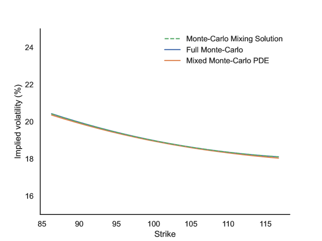
Figure 1. The implied volatility curve in the Inverse-Gamma model. The number of Monte-Carlo paths for the Monte-Carlo Mixing Solution, Full Monte-Carlo and mixed Monte-Carlo PDE methods are $10\times 10^{5},15\times 10^{5},10\times 10^{4}$ respectively, whereas the number of time steps are $24,48$ and $1$ per day respectively.

Figure 1 shows a plot of the implied volatility curve obtained from all three methods in the Inverse-Gamma model with the aforementioned parameters. One can see qualitatively that the mixed Monte-Carlo PDE method does indeed reproduce the implied volatility curve well. More detailed and quantitative numerical results are provided in Appendix C.

One will note that for the two methods, there is ostensibly a mismatch between the number of time-steps per day and paths chosen in our numerical experiments in Tables C.2 and C.3. However, this is not necessarily the case. First, it does not seem appropriate to directly compare the number of time-steps utilised by these two methods, since the mixed Monte-Carlo PDE method requires a time discretisation of $V$ as well as the SPDE, however the Full Monte-Carlo method requires a time discretisation of both $V$ and $X$. Secondly, the apparent mismatch between the number of paths considered for the two methods can be easily clarified as well. Via properties of conditional expectation, one can show that given a number of paths, the Monte-Carlo standard error for the mixed Monte-Carlo PDE method is significantly less than that of the Full Monte-Carlo method. Intuitively this makes sense; simulation of $X$ usually contributes the most to the Monte-Carlo variance, however in our mixed Monte-Carlo method we bypass simulation of $X$ by offloading it to the PDE component. In fact this highlights a substantial advantage of our mixed Monte-Carlo PDE method; bluntly speaking the PDE component does the hard work by handling $X$, whereas the Monte-Carlo component does the easier work by tackling $V$.

At first glance it may seem that the run times of the mixed Monte-Carlo PDE method pale in comparison to the Full Monte-Carlo method. However these are not at all comparable, as another significant advantage of the mixed Monte-Carlo PDE method is that as it is a PDE method, we obtain the price of the put option for various $S_{0}$ values (250 values in this case!), whereas the Full Monte-Carlo method only obtains it for a single value.

For the mixed Monte-Carlo PDE method, we have considered a special case where we utilise 1,000,000 paths for each choice of #Steps/day. This is in an attempt to reduce the Monte-Carlo standard error sufficiently low so that it is negligible compared to the time and space discretisation error, thereby giving us a better idea of what the combined time and space discretisation errors solely are. For the Full Monte-Carlo method, we have proceeded in a similar manner, where we have considered a case with 10,000,000 paths for each choice of #Steps/day.

As mentioned above, it is difficult to compare the errors between the two methods as their number of time-steps per day and paths do not have a direct correspondance. However, we have selected them as best as we believe possible in order to draw a fair comparison. The Full Monte-Carlo errors in Table C.3 are standard and require no further investigation. For the mixed Monte-Carlo PDE method results in Table C.2, the absolute errors and standard errors are at most approximately 10 basis points, which is more than sufficient in application. One thing to note is that it seems to have an unpredictable error for #Steps/day = 0.5, meaning that the absolute error is not decreasing very monotonically as the number of paths increase. However, it starts to settle down for #Steps/day = 1, 2. It seems logical to attribute this consistency to the PDE solver being sufficiently accurate on these finer time grids.

7. Conclusion

In this article we have proved a conditional Feynman-Kac formula which arises in the context of mathematical finance, and proved under certain assumptions that the existence and uniqueness of the associated SPDE is valid. These results are similar to results obtained in Section 6 of [10], however in our case, non-trivialities arise due to the backward Brownian motion and backward filtration that must be considered, namely $\mathring{B}$ and $(\bar{\mathcal{F}}_{t,T}^{V,B})_{t\in[0,T]}$. Under additional assumptions on the speed of growth of the density of the auxiliary process $V$, we have shown that Pardoux’s results can be adapted to the setting considered in this article. The purpose of developing this conditional Feynman-Kac formula is to utilise it to solve problems in mathematical finance. Indeed, we demonstrate its application in the simple setting of pricing a European put option in the Inverse-Gamma model. The conditional Feynman-Kac formula can be applied in other settings in mathematical finance, for example, mixing Least Square Monte-Carlo methods with numerical PDE methods, which will be the focus of forthcoming articles.

Appendix A Some content on backward stochastic calculus

In this appendix, we provide the definitions of the backward versions of common objects and concepts from stochastic calculus. These definitions are obvious counterparts to their forward versions.

Definition A.1 (Backward filtration).

Let $(\mathcal{G}_{t,T})_{t\in[0,T]}$ be a decreasing collection of $\sigma$-algebras. Then $(\mathcal{G}_{t,T})_{t\in[0,T]}$ is called a backward filtration. We assume all backward filtrations considered satisfy the usual conditions, which for backward filtrations are: left continuity, i.e., $\mathcal{G}_{t,T}=\bigcap_{\varepsilon>0}\mathcal{G}_{t-\varepsilon,T}$ for all $t\in[0,T]$, and also that $\mathcal{G}_{T,T}$ is augmented by null sets.

Definition A.2 (Backward martingale).

Consider a process $M$ as well as a backward filtration $(\mathcal{G}_{t,T})_{t\in[0,T]}$. Suppose $M$ satisfies the following.

1. $M$ is adapted to the backward filtration $(\mathcal{G}_{t,T})_{t\in[0,T]}$.

2. $\mathbb{E}|M_{t}|<\infty$ for all $t\in[0,T]$.

3. $\mathbb{E}[M_{s}|\mathcal{G}_{t,T}]=M_{t}$ for $s<t$.

Then $M$ is called a backward martingale w.r.t. the backward filtration $(\mathcal{G}_{t,T})_{t\in[0,T]}$.

Definition A.3 (Backwards stopping time).

Consider a backward filtration $(\mathcal{G}_{t,T})_{t\in[0,T]}$. The random variable $\tau:\Omega\to\mathbb{R}$ is called a backward stopping time if the events $\{\tau\geq t\}\in\mathcal{G}_{t,T}$ for each $t$.

Definition A.4 (Backward local-martingale).

Consider a process $M$ which is adapted to a backward filtration $(\mathcal{G}_{t,T})_{t\in[0,T]}$. Let $(\tau_{n})_{n}$ be a sequence of backward stopping times with respect to $(\mathcal{G}_{t,T})_{t\in[0,T]}$ such that

1. $\tau_{n}\downarrow 0$ a.s.

2. $(\tau_{n})_{n}$ is non-increasing a.s.

Suppose that $M_{t}^{(n)}:=M_{t\vee{\tau_{n}}}$ is a $(\mathcal{G}_{t,T})_{t\in[0,T]}$ backward martingale for each $n$. Then $M$ is called a backward local-martingale relative to $(\mathcal{G}_{t,T})_{t\in[0,T]}$.

Definition A.5 (Backward Brownian motion).

Consider a process $Z$ taking values in $\mathbb{R}^{d}$ which is adapted to a backward filtration $(\mathcal{G}_{t,T})_{t\in[0,T]}$. In addition, let $Z$ satisfy the following:

1. $Z$ is continuous in $t$ a.s.

2. For $t>s$, the increment $Z_{s}-Z_{t}\sim\mathcal{N}(0,(t-s)I)$ where $I$ is the $d\times d$ identity matrix.

3. For $t>s$, the increment $Z_{s}-Z_{t}$ is independent of $\mathcal{G}_{t,T}$.

Then $Z$ is called a backward Brownian motion relative to $(\mathcal{G}_{t,T})_{t\in[0,T]}$. Moreover, if $Z_{T}=0$, then $Z$ is called a standard backward Brownian motion relative to $(\mathcal{G}_{t,T})_{t\in[0,T]}$.

Remark A.1.

It is clear that a backward Brownian motion is a backward martingale.

Remark A.2.

It is clear that Levy’s characterisation of Brownian motion extends to the backward scenario. Namely, a stochastic process is a backward Brownian motion if and only if it is a backward local-martingale with quadratic variation $t$.

Appendix B Supplementary results

In this section, we provide some supplementary results required for the proofs of the results in this article. We remark that Theorem B.1 is Theorem 2.2 in [11], we state it here for convenience to the reader.

Theorem B.1 (Theorem 2.2 in [11]).

Enforce mB. Recall from Section 5 that $\bar{\mathcal{F}}^{V,B}_{t,T}:=\mathcal{F}^{B}_{t,T}\vee\sigma(V_{t})$ and

$$\mathring{B}_{t}^{k}=B_{t}^{k}-B_{T}^{k}-\int_{t}^{T}\frac{\sum_{l=1}^{D}\partial_{y_{l}}(p(r,V_{r})\beta_{l,i}(r,V_{r}))}{p(r,V_{r})}\mathrm{d}r,\quad k=1,\dots,D,$$

where the integrand is taken to be zero if ever $p$ is zero. Then $\mathring{B}$ is a $\mathbb{R}^{D}$ valued backward Brownian motion in $(\bar{\mathcal{F}}_{t,T}^{V,B})_{t\in[0,T]}$.

Proposition B.1.

Let $X=(X_{1},\dots,X_{D})$ be a $\mathbb{R}^{D}$ valued random vector with density $p_{X}(x)$ and define $X\wedge C=(X_{1}\wedge C,\dots,X_{D}\wedge C)$ for some constant $C>0$. Denote the density of $X\wedge C$ by $p_{X}^{C}(x)$. Then

$$\int_{\mathbb{R}^{D}}|x|^{2p}p_{X}^{C}(x)\mathrm{d}x\leq D^{p}C^{2p}$$

for $p\geq 0$.

Outline of proof.

We will give an outline of the proof, as the full proof is rather long and not the intention of this article. The idea however is to explicitly characterise the density $p_{X}^{C}(x)$. We do so by defining the following events:

$$A_{i}^{1} :=\{x_{i}\leq X_{i}\leq x_{i}+\mathrm{d}x_{i},C\geq x_{i}\},$$

$$A_{i}^{2} :=\{x_{i}\leq C\leq x_{i}+\mathrm{d}x_{i},X_{i}\geq x_{i}\}.$$

Then

$$\bigcap_{i=1}^{D}\{x_{i}\leq X_{i}\wedge C\leq x_{i}+\mathrm{d}x_{i}\}=\bigcap_{i=1}^{D}A_{i}^{1}\cup A_{i}^{2}=\bigcup_{j_{1},\dots,j_{D}\in\{1,2\}}\bigcap_{i=1}^{D}A_{i}^{j_{i}}.$$

Hence we are interested in studying the probability of the event $\bigcap_{i=1}^{D}A_{i}^{j_{i}}$. First note that for $j_{i}=1$ with $i=1,\dots,D$ we have

$$\mathbb{P}\left(\bigcap_{i=1}^{D}A_{i}^{1}\right)=p_{X}(x)\mathrm{d}x\textbf{1}_{\{\max(x_{1},\dots,x_{D})\leq C\}}$$

and for $j_{i}=2$ with $i=1,\dots,D$ we have

$$\mathbb{P}\left(\bigcap_{i=1}^{D}A_{i}^{2}\right)=\left(\prod_{i=1}^{D}\delta(C-x_{i})\right)\mathrm{d}x\mathbb{P}\left(\bigcap_{i=1}^{D}\{X_{i}\geq x_{i}\}\right).$$

For a generic string $(j_{1},\dots,j_{D})\in\{1,2\}^{D}$ the probability is more difficult to write down notationally. However, it is simple when considering specific strings. For example when $D=3$ and $j_{1}=j_{2}=1$ and $j_{3}=2$ we get

$$\mathbb{P}\left(\bigcap_{i=1}^{3}A_{i}^{j_{i}}\right)=p(x_{1},x_{2},X_{3}\geq x_{3})\textbf{1}_{\{x_{1}\leq C,x_{2}\leq C\}}\delta(C-x_{3}),$$

where

$$p(x_{1},x_{2},X_{3}\geq x_{3})\mathrm{d}x_{1}\mathrm{d}x_{2}=\mathbb{P}(x_{1}\leq X_{1}\leq x_{1}+\mathrm{d}x_{1},x_{2}\leq X_{2}\leq x_{2}+\mathrm{d}x_{2},X_{3}\geq x_{3})$$

for small $\mathrm{d}x_{1}\mathrm{d}x_{2}$. Knowing that it is possible to write down the probability of the event $\bigcap_{i=1}^{D}A_{i}^{j_{i}}$ for any string $(j_{1},\dots,j_{D})\in\{1,2\}^{D}$, this suffices for writing down the density $p_{X}^{C}(x)$. The bound claimed in the proposition is obtained by merely appealing to this form of the density. ∎

Appendix C Numerical results

Table C.1. Implied volatility, Monte-Carlo standard error, and Run time for pricing an ATM Put option with maturity 6 months. Price is obtained via the Monte-Carlo Mixing Solution method with 1,000,000 paths and 24 time steps per day (Benchmark).

Benchmark
#Steps/day	#Path		IV(%)	S.E.(bp)	Abs Err(bp)	Run(s)
24	$10\times 10^{5}$		18.872	1.20	N/A	226.7

Table C.2. Implied volatilities, Monte-Carlo standard errors, Absolute errors, and Run times for pricing an ATM Put option with maturity 6 months via the mixed Monte-Carlo PDE method, where # of paths and time steps per day are varied, and # of space points is fixed at 250.

Mixed Monte-Carlo PDE
#Steps/day	#Path		IV(%)	S.E.(bp)	Abs Err(bp)	Run(s)
0.5	$10\times 10^{3}$		18.77	11.71	9.72	74.6
	$20\times 10^{3}$		18.99	8.51	11.35	148.9
	$40\times 10^{3}$		18.87	5.95	0.09	298.7
	$80\times 10^{3}$		18.85	4.21	2.03	595.7
	$10\times 10^{5}$		18.91	1.20	3.85	7404.3
1	$10\times 10^{3}$		18.79	11.71	8.27	147.9
	$20\times 10^{3}$		18.85	8.57	1.68	295.2
	$40\times 10^{3}$		18.83	5.95	3.80	589.0
	$80\times 10^{3}$		18.87	4.20	0.40	1177.0
	$10\times 10^{5}$		18.88	1.19	0.48	14712.6
2	$10\times 10^{3}$		18.96	12.09	8.85	297.7
	$20\times 10^{3}$		18.84	8.36	3.28	597.8
	$40\times 10^{3}$		18.80	5.88	6.82	1184.0
	$80\times 10^{3}$		18.87	4.23	0.02	2376.3
	$10\times 10^{5}$		18.89	1.19	1.52	29642.8

Table C.3. Implied volatilities, Monte-Carlo standard errors, Absolute errors, and Run times for pricing an ATM Put option with maturity 6 months via the Full Monte-Carlo method, where the number of paths and time steps per day are varied.

Full Monte-Carlo
#Steps/day	#Path		IV(%)	S.E.(bp)	Abs Err(bp)	Run(s)
0.5	$40\times 10^{3}$		18.89	14.55	2.20	0.20
	$80\times 10^{3}$		19.09	10.34	22.08	0.41
	$160\times 10^{3}$		18.93	7.27	5.66	1.24
	$320\times 10^{3}$		18.97	5.14	9.97	2.59
	$100\times 10^{5}$		19.00	0.92	12.51	77.50
1	$40\times 10^{3}$		18.93	14.51	5.83	0.41
	$80\times 10^{3}$		18.90	10.26	3.25	0.82
	$160\times 10^{3}$		18.84	7.26	3.04	2.41
	$320\times 10^{3}$		18.93	5.13	6.32	4.83
	$100\times 10^{5}$		18.95	0.92	7.48	156.52
2	$40\times 10^{3}$		18.67	14.41	20.04	0.82
	$80\times 10^{3}$		18.86	10.25	1.29	1.65
	$160\times 10^{3}$		18.93	7.26	5.56	4.86
	$320\times 10^{3}$		18.93	5.14	6.09	9.61
	$100\times 10^{5}$		18.91	0.92	3.57	310.92
4	$40\times 10^{3}$		18.85	14.39	2.33	1.62
	$80\times 10^{3}$		18.92	10.22	4.91	3.45
	$160\times 10^{3}$		18.77	7.22	9.73	9.74
	$320\times 10^{3}$		18.89	5.12	2.30	19.18
	$100\times 10^{5}$		18.89	0.92	1.38	624.10
8	$40\times 10^{3}$		18.81	14.48	6.55	3.22
	$80\times 10^{3}$		18.89	10.23	1.83	6.58
	$160\times 10^{3}$		18.74	7.20	13.56	19.36
	$320\times 10^{3}$		18.82	5.11	4.89	38.27
	$100\times 10^{5}$		18.88	0.92	0.84	1242.32
16	$40\times 10^{3}$		18.76	14.42	10.81	6.47
	$80\times 10^{3}$		18.85	10.22	2.51	13.01
	$160\times 10^{3}$		18.99	7.27	12.14	38.70
	$320\times 10^{3}$		18.93	5.13	5.91	76.65
	$100\times 10^{5}$		18.85	0.92	1.91	2477.73
24	$40\times 10^{3}$		18.86	14.40	1.18	9.63
	$80\times 10^{3}$		18.88	10.25	0.40	19.58
	$160\times 10^{3}$		18.98	7.28	10.56	57.93
	$320\times 10^{3}$		18.85	5.11	2.13	115.06
	$100\times 10^{5}$		18.86	0.92	0.74	3718.76

References

• [1] Kaustav Das. mixed_MC_PDE, 2023. doi:10.5281/zenodo.10171222.
• [2] Kaustav Das and Nicolas Langrené. Closed-form approximations with respect to the mixing solution for option pricing under stochastic volatility. Stochastics, 94(5):745–788, 2022.
• [3] Lawrence C Evans. Partial differential equations, volume 19. American Mathematical Soc., 2010.
• [4] Jonathan Ho, Ajay Jain, and Pieter Abbeel. Denoising diffusion probabilistic models. Advances in neural information processing systems, 33:6840–6851, 2020.
• [5] Nikolai Vladimirovich Krylov and Boris Lvovich Rozovskiĭ. Stochastic partial differential equations and diffusion processes. Russian Mathematical Surveys, 37(6):81–105, 1982.
• [6] Hiroshi Kunita. Stochastic partial differential equations connected with non-linear filtering. In Nonlinear filtering and stochastic control, pages 100–169. Springer, Berlin, Heidelberg, 1982.
• [7] Nicolas Langrené, Geoffrey Lee, and Zili Zhu. Switching to nonaffine stochastic volatility: A closed-form expansion for the Inverse Gamma model. International Journal of Theoretical and Applied Finance, 19(05):1650031, 2016.
• [8] Daniel Ocone and Etienne Pardoux. A stochastic Feynman-Kac formula for anticipating SPDE’s, and application to nonlinear smoothing. Stochastics: An International Journal of Probability and Stochastic Processes, 45(1-2):79–126, 1993.
• [9] Etienne Pardoux. Stochastic partial differential equations and filtering of diffusion processes. Stochastics, 3(1-4):127–167, 1979.
• [10] Etienne Pardoux. Équations du filtrage non linéaire de la prédiction et du lissage. Stochastics, 6(3-4):193–231, 1982.
• [11] Etienne Pardoux. Grossissement d’une filtration et retournement du temps d’une diffusion. In Séminaire de Probabilités XX 1984/85, pages 48–55. Springer, 1986.
• [12] Daniel W Stroock and SR Srinivasa Varadhan. Multidimensional diffusion processes, volume 233. Springer Science & Business Media, 1997.
• [13] Toshio Yamada and Shinzo Watanabe. On the uniqueness of solutions of stochastic differential equations. Journal of Mathematics of Kyoto University, 11(1):155–167, 1971.