Nonunique Stationary States and Broken Universality in Birth Death Diffusion Processes

Abstract

Systems with absorbing configurations usually lead to a unique stationary probability measure called quasi stationary state (QSS) defined with respect to the survived samples. We show that the birth death diffusion (BBD) processes exhibit universal phases and phase transitions when the birth and death rates depend on the instantaneous particle density and their time scales are exponentially separated from the diffusion rates. In absence of birth, these models exhibit non-unique QSSs and lead to an absorbing phase transition (APT) at some critical nonzero death rate; the usual notion of universality is broken as the critical exponents of APT here depend on the initial density distribution.

Markovian dynamics is used extensively in Physics, Chemistry, Biology, Economics, and many other branches of science to model real-world processes, both in equilibrium and nonequilibrium conditions [1, 2]. Lattice models in thermal equilibrium [3, 4, 5] are usually described by Markov processes (MPs) known as Monte Carlo dynamics, a dynamics that obeys detailed balance condition w.r.t. Gibbs measure, and they have found vast application in polymer physics [6], active and granular media [7], traffic flows [8], protein folding [9] etc.. In the absence of Gibbs measure, nonequilibrium systems are primarily described by Markov jump processes [10] and they exhibit novel nonequilibrium phases, and phase transitions [12, 11]. Ergodicity is crucial for MPs to attain a unique steady state, which is trivially broken if the system has absorbing configurations -the configurations where the system is permanently trapped once reached. The stationary measure of models with absorbing configurations are trivial: the steady-state probability for the system to be any configuration except the absorbing one is zero. An important question is to find a probability measure for the quasi-stationary state (QSS) defined w.r.t. the survived (no absorbed) samples. Simple models like contact process [13], directed percolation [14, 15], pair contact process [16], and fixed energy sandpiles [17, 18, 19] are known to have unique QSSs and they exhibit absorbing phase transitions (APT); some of them are realized experimentally [20, 21].

In this letter, we study absorbing-state phase transition in a simple Birth-Death-Diffusion (BDD) process where birth and death rates depend on the instantanuous particle density. We find that irrespective of the nature of diffusing(conserving) dynamics, these models exhibit APT when death rates crosses a critical threshold. In absence of birth, the QSS becomes non-unique in the sense that the probability measure there depends on the the initial conditions. The nonuniqueness persists at the critical point resulting in initial condition dependence of the standard critical exponents. We provide A sufficient criteria for the system to have such nonunique QSSs.

The model: Let us associate particle deposition (birth) and evaporation (death) dynamics

$$1\xrightleftharpoons[B(\rho)]{D(\rho)}0,$$ (1)

to an one dimensional system of size $L$ which otherwise follows a particle conserving dynamics. The rates $B(.)$ and $D(.)$ are analytic functions of instantaneous particle density $\rho=\frac{N}{L},$ where $N$ is the number of particles. In particular, we are interested in rate functions of the form $D(\rho)=e^{-L\theta(\rho)}$, and $B(\rho)=\rho e^{-L\phi(\rho)};$ $B(0)=0$ ensures that an empty lattice is the only absorbing configuration of the system. Along with these birth-death dynamics (1), we assume the system to have a natural conserving dynamics; the simplest one being the symmetric exclusion process (SEP) on a one-dimensional periodic lattice labeled $i=1,2...,L,$ with $s_{i}=0,1$ representing occupancy of the site $i.$

$$10\xrightleftharpoons[1]{1}01.$$ (2)

In absence of birth and death, the conserving dynamics leads the system having $N$ particles to a stationary probability measure $g_{N}(\mathcal{C})$; for SEP in Eq. (2), $g_{N}(\mathcal{C})=\binom{L}{N}^{-1}$ is a constant.

The birth-death rates in BBD model, being extremely slow (${\mathcal{O}}(e^{-L})$) compared to the conserved dynamics (${\mathcal{O}}(1)$), effectuates a separation of timescales between the particle conserving and particle non-conserving dynamics. Between any two density-altering events $N\to N\pm 1,$ the system gets enough time to equilibriate to the stationary distribution $g_{N}(\mathcal{C}).$ This separation of time scale decouples the conserved and nonconserved part of the dynamics, making the nonconserved dynamics effectively a biased walk (RW) on $N=0,1,2,\dots L,$ with an absorbing boundary at $N=0.$

$$N-1\xleftarrow[]{D_{N}}N\xrightarrow[]{B_{N}}N+1,$$ (3)

where $B_{N}=(L-N)B(\rho)$ and $D_{N}=ND(\rho)$ where $\rho\equiv\frac{N}{L}$. The additional multiplicative factors in birth and death rates are natural to expect as in any configuration having $N$ particles, death (of a particle) can occur at any of the $N$ sites whereas birth can occur at $L-N$ sites. If the QSS of this absorbing RW is $\{f_{N}\}$, $N=1,2,\dots L,$ then the same for the whole system can be written assuming a good separation of time scale as, $P(\mathcal{C})=f_{N}g_{N}(\mathcal{C}),{\rm where}~{}N\equiv N(\mathcal{C})$

Absorbing phase transition (APT): When the time-scales are well separated, the steady state density of the system can be determined completely from the QSS of the RW. Corresponding APT if any, and its critical behaviour, are the governed solely by the birth-death dynamics, irrespective of the nature of the diffusive (conserving) dynamics. But, will there be any APT? Consider a region of parameter space where $B_{N}>D_{N}\ \forall\ N\in(0,L).$ Here the system is drifted towards higher density. Since $B_{N}=e^{-L\phi(\rho)+\ln L(1-\rho)}\simeq B(\rho)$ and similarly $D_{N}\simeq D(\rho),$ for any density $0<\rho<1$ one can make $B(\rho)\gg D(\rho)$ by increasing $L$. Then, a super fast drift towards higher density will pin the walker at $\rho=1.$ On the other hand, for $D_{N}>B_{N}$ the system drifts towards $\rho=0$ and thus most walkers are absorbed; those who survive will contribute to the QSS. Most of the survived walker will be found at some $N^{*}=\rho^{*}L$ where the dynamics is slowest or the waiting time is large, i.e. where $B_{N}+D_{N}$ has its minimum. $\rho^{*}$ can be tuned continuously by birth and death rates to obtain an absorbing transition in thermodynamically large systems when $\rho^{*}$ falls below $\frac{1}{L}$ (i.e., $\rho\to 0$).

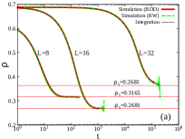
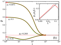
Figure 1: (Color online) Decay of $\rho(t)$, (a) for different $L=8,16,32,$ with initial density $\rho_{i}=0.7$ ($N=\lfloor 0.7L\rfloor$) and (b) different initial conditions $\rho_{i}=\frac{11}{16},\frac{1}{2},\frac{1}{4}$ for $L=16.$ Three different overlapping curves corresponds to Monte Carlo simulation of the BBD model for $b=1.4,d=0.6$ (solid red line), simulation of an effective RW dynamics (dashed green line) and numerical integration of the Master equation for the RW (dotted black line). The horizontal lines are the value of $\rho_{s}$ obtained from a QSS simulation proposed in Ref. [22]. Inset of (b) shows that indeed $\rho_{s}\to d=0.6$ following Eq. (5) when $L\to\infty;$ asymptotically, $\rho_{s}-\rho_{s}(L)\sim L^{-0.428}$ (dashed line).

Let us consider a specific example. Along with the conserving dynamics SEP in Eq. (2), we consider dynamics (1) with

$$D(\rho)=e^{-L\rho(2d-\rho)};\quad B(\rho)=\rho e^{-L\rho(2/b-\rho)},$$ (4)

which have two real parameters $b$ and $d.$ We take $b\geq 0$ as $B(\rho)$ can not be analytically continued to $b<0.$ First let us check whether the time-scales are well separated. In Fig. 1(a) we plot $\rho(t)$ for $b=1.4,d=0.6$ obtained from Monte Carlo simulations of the model for $L=8,16,32$ and compared them with $\rho(t)$ obtained from simulations of the biases RW dynamics (3). For small systems, the Master equation for the absorbing RW can be integrated numerically to obtain $\rho(t),$ which is also plotted in Fig. 1. An excellent match of all three curves justifies the separation of time scale and the decoupling of the non-conserved dynamics from the conserved one.

For rates (4), $B_{N}>D_{N}$ corresponds to $bd>1.$ In this regime we expect the steady state density to be $\rho_{s}=1.$ For $bd<1,$ $\frac{1}{L}(D_{N}+B_{N})=(1-\rho)B(\rho)+\rho D(\rho),$ which has its minimum at $\rho^{*}=d.$ Thus based on these phenomenological arguments,

$$\rho_{s}=\begin{cases*}0&$d<0$\\ d&$0\leq d<1$ \& $bd\leq 1$\\ 1&otherwise\end{cases*}.$$ (5)

This result, of course, can be shown rigorously (see Supplemental Material).

With $\rho_{s}$ in hand, we can proceed to obtain the phase diagram in $b$-$d$ plane. But there is a problem. For $b=1.4,d=0.6,$ we have obtained the steady state density $\langle\rho\rangle\equiv\rho_{s}$ for different $L$ in Fig. 1; $\rho_{s}$ for the largest $L=32$ was found found to be $0.364$ which is far way from the analytical result $\rho_{s}=0.6,$ in (5). The non-monotonic $L$ dependence of $\rho_{S}(L)$ adds more doubt on whether $\rho_{S}(L)\to d$ as $L\to\infty.$ Moreover, simulation for larger $L$ takes astronomically large time as the waiting times are ${\mathcal{O}}(e^{L}).$ Fortunately a recently proposed simulation method for QSS [22] helps us to obtain $\rho_{s}$ for reasonably large $L.$ The inset of Fig. 1, for $b=1.4,d=0.6,$ shows that indeed $\rho_{s}$ approaches $d=0.6$ following an asymptotic power-law, $\rho_{s}=0.6-L^{-0.428}.$

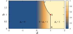
Figure 2: (Color online) Three phases of BBD model: $\rho=0$ (absorbing) $0<\rho<1$ (active) and $\rho=1$ (maximal density). The APT occurs at $d=0.$ On PQR line $\bar{\rho}_{s}=1-\rho_{s}$ exhibits an ordinary phase transition, continuous (discontinuous) along QR(PQ) segments with a tricritical point $b=1=d$ (Q).

The phase diagram, based on Eq. (5), is shown in Fig. 2 where $0<\rho_{s}<1$ region is separated from two other regions $\rho_{s}=0$ and $\rho_{s}=1.$ The BBD model exhibits continuous absorbing-state phase transition at $d=0$ line. For a fixed value of $b$, $\rho_{s}$ decreases continuously with decrease of $d$ until a critical threshold $d_{c}=0$ is reached. Surprisingly, an ordinary non-equilibrium phase transition also takes place along PQR line in Fig 2. The order parameter $\bar{\rho}_{s}=1-\rho_{s}$ picks up a nonzero value when, for a fixed $b,$ $d$ is decreased below

$$\bar{d}_{c}=\begin{cases}1&0<b<1\\ b^{-1}&b\geq 1.\end{cases}$$ (6)

This transition is discontinuous when $b\in(1,\infty)$ (along PQ line in Fig. 2) as $\bar{\rho}_{s}$ jumps from $0$ to $1-\frac{1}{b}$ at $d=\bar{d}_{c}$, whereas it is continuous $b\in(0,1],$ leading to the fact that Q ($(d,b)=(1,1)$) is a tri-critical point.

The line $b=0$ corresponds to no birth of particles. In this case, we can solve the master equation of the system exactly. Let us assume that in absence of birth and death, the diffusive dynamics follows a master equation $\frac{d}{dt}|\phi_{N}\rangle=\mathbf{C}_{N}|\phi_{N}\rangle$ with $N=0,1,\dots,L$ conserved. $|\phi_{N}\rangle$ is a $\binom{L}{N}$ dimensional vector with components representing the probability of being in $\binom{L}{N}$ configurations of the conserved system. For $N=0,L$ the system has only one configuration and evolution has no meaning; we set the scalars $\mathbf{C}_{0}=0=\mathbf{C}_{L}$ for notational convenience. We also denote the steady states as $|\bar{\phi}_{N}\rangle$ which satisfy $\mathbf{C}_{N}|\bar{\phi}_{N}\rangle=0.$ Now the master equation on $b=0$ line can be written as $\frac{d}{dt}|P\rangle=\mathbf{M}|P\rangle$ with $|P\rangle=(|\phi_{0}\rangle,|\phi_{1}\rangle,\dots,|\phi_{L}\rangle)^{T}$ and $\mathbf{M}$ in block-form reads,

$$\mathbf{M}=\begin{pmatrix}\mathbf{M}_{0}&D_{1}\mathbf{T}_{1}&\mathbf{0}&\mathbf{0}&\dots&\mathbf{0}\\ \mathbf{0}&\mathbf{M}_{1}&D_{2}\mathbf{T}_{2}&\mathbf{0}&\dots&\mathbf{0}\\ \mathbf{0}&\mathbf{0}&\mathbf{M}_{2}&D_{3}\mathbf{T}_{3}&\dots&\mathbf{0}\\ \vdots&\vdots&\vdots&\vdots&\ddots&\vdots\\ \mathbf{0}&\mathbf{0}&\mathbf{0}&\mathbf{0}&\dots&\mathbf{M}_{L}\end{pmatrix}.$$ (7)

Here $\textbf{M}_{n}=\mathbf{C}_{n}-nD_{n}\mathbf{I}_{n}$ are $\binom{L}{n}$ dimensional square matrices with $D_{n}\equiv D(n/L)$ and $\mathbf{I}_{n}$ is the identity matrix; obviously $\textbf{M}_{0}=0$ is a scalar. The $\mathbf{T}_{n}$s are $\binom{L}{n-1}\times\binom{L}{n}$ matrices such that each column has exactly $n$ number of $1$s corresponding to a surjective mapping of $n$-particle configurations to $n-1$ particle configurations, $\mathcal{C}_{n}\mapsto\mathcal{C}_{n-1}$, by operation of removal of a single particle without disturbing any other particle. Clearly the eigenvalues of this upper triangular block matrix $\mathbf{M}$ are $\Lambda[\mathbf{M}]=\bigcup_{n}\Lambda[\mathbf{M_{n}}].$ In other words, the set of $2^{L}$ eigenvalues of $\mathbf{M}$ are $\lambda_{n\nu}=\Lambda[\mathbf{C}_{n}]_{\nu}-nD_{n},$ where $\Lambda[\mathbf{C}_{n}]_{\nu}$ are $\nu^{th}$ eigenvalue of $\mathbf{C}_{n}$ in a decreasing order and $\nu=0,1,\dots\binom{L}{n}$ for any given $n.$ It is now straight forward to calculate both the left and right eigenvectors of $\lambda_{n\nu},$ respectively $\langle\Psi_{n\nu}|$ and $|\Psi_{n\nu}\rangle.$ For our purpose calculating them for $\nu=0$ are enough (see text below).

$$\langle\Psi_{n0}| = \left(\langle\psi_{0}|,\langle\psi_{1}|,\dots\right);~{}~{}|\Psi_{n0}\rangle=\left(|\psi_{0}\rangle,|\psi_{1}\rangle,\dots\right)^{T}$$ (8)

$$\langle\psi_{k}| = \begin{cases}\mathbf{0}&k<n\\ \langle 1_{k}|\prod_{i=n+1}^{k}\frac{\lambda_{i0}}{\lambda_{i0}-\lambda_{n0}}&k\geq n\end{cases}$$ (9)

$$|\psi_{k}\rangle = \begin{cases}\prod_{i=1}^{n-1}\frac{\lambda_{i0}}{\lambda_{n0}-\lambda_{i0}}&k=0\\ \prod_{i=k+1}^{n}\frac{\lambda_{i0}}{i}(\mathbf{M}_{i-1}-\lambda_{n0})^{-1}\mathbf{T}_{i}|\bar{\phi}_{n}\rangle&0<k\leq n\\ \mathbf{0}&k>n\end{cases}$$

where ${\mathbf{0}}$ are null vectors and $\langle 1_{k}|\equiv(1,1,\dots)$ in $\binom{L}{k}$ dimension.

The probability $Q_{mn}$ that system, starting from a configuration with $m$ number of particles at $t=0,$ is not absorbed until time $t$ and it has $n$ particles is

$$Q_{mn}(t)=\frac{\langle n|e^{\mathbf{M}t}|m\rangle}{1-\langle 0|e^{\mathbf{M}t}|m\rangle}=\frac{\sum\limits_{k\neq 0}e^{-kD_{k}t}\langle n|\Psi_{k0}\rangle\langle\Psi_{k0}|m\rangle}{-\sum\limits_{k\neq 0}e^{-kD_{k}t}\langle 0|\Psi_{k0}\rangle\langle\Psi_{k0}|m\rangle}$$ (10)

where, in the spectral decomposition we kept only the dominant eigenvectors (corresponding to $\lambda_{m0}$). We also denote $\langle m|=\binom{L}{m}^{-1}({\mathbf{0},0},\dots,|1_{m}\rangle,\dots,{\mathbf{0}})$ and $|m\rangle=\langle m|^{T}.$ Clearly $|m\rangle$ represents a state of the system where all configurations that has exactly $m$ particles are equally likely. Note that, $\langle m|$ is a left eigenvector of any Markov matrix in $\binom{L}{m}$ dimension, whereas $|m\rangle$ is the steady state for certain specific dynamics, like the SEP defined in (2), where all configurations are equally likely in steady state.

In the long time limit, one of the term $k=\bar{k}=\arg\min\limits_{k>0}(kD_{k})~{}\forall~{}k$ is dominant in the sums that appear in $Q_{mn}$ as long as $\langle\Psi_{k}|m\rangle\neq 0,$ leading to,

$$\small Q_{mn}=\frac{\langle n|\Psi_{\bar{k}0}\rangle}{-\langle 0|\Psi_{\bar{k}0}\rangle}=\begin{cases}\frac{\bar{k}D_{\bar{k}}}{nD_{n}}\prod\limits_{k<\bar{k}}\left(1-\frac{\bar{k}D_{\bar{k}}}{kD_{k}}\right)&n\leq\bar{k}\\ 0&\bar{k}<n\end{cases}.$$ (11)

It appears that $Q_{mn}$ for $b=0$ does not depend on the initial density $m/L,$ however that is not true. Unlike $b>0$ case where $\langle\Psi_{1}|m\rangle\neq 0~{}\forall~{}m$, here it is evident from Eq. (9) that $\langle\Psi_{1}|m\rangle$ may become zero for some choice of $m$ leading to a possibility of a non-unique QSS that depends on the initial condition.

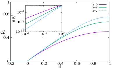
Figure 3: (Color online) $\rho_{s}$ and its fluctuation $\Delta\rho_{s}^{2}$ (in the inset) vs. $d$ for different initial density distributions $\pi(\rho)=(1+a)\rho^{a}$, $a=0,1,2$. For $d_{c}\approx 0,$ $\rho_{s}\sim d^{\beta}$ and $\Delta\rho_{s}^{2}\sim d^{-\gamma};$ the critical exponent $\gamma=-(a+3)$ depends on initial condition, whereas $\beta$ does not.

In continuum limit, we denote $(m,n,\bar{k})=(\rho_{i},\rho,\rho^{*})L$ and thus the Matrix $Q_{mn}$ takes functional form

$$Q(\rho_{i},\rho)=e^{2Ld(\rho-\rho^{*})}\Theta(\rho^{*}-\rho),$$ (12)

which is the probability that a non-absorbed (or survived) system has steady state density $\rho,$ when it is initialized at density $\rho_{i}.$ For an arbitrary initial density distribution $\pi(\rho_{i})$ with $\rho_{i}>0$ the QSS measure is ${\cal Q}(\rho)=\int_{0^{+}}^{1}\mathrm{d}\rho_{i}Q(\rho_{i},\rho)\pi(\rho_{i})$ and the steady state density, calculated using Laplace method [23], is

$$\langle\rho\rangle=\int_{0}^{1}\mathrm{d}\rho\mathcal{Q}(\rho)\rho\approx\int_{0}^{1}\mathrm{d}\rho_{i}\pi(\rho_{i})\rho^{*};~{}\rho^{*}=\begin{cases}\rho_{i}&\rho_{i}\leq d\\ d&\rho_{i}>d\geq 0\\ 0&d<0\end{cases}.$$ (13)

Let us consider $\pi(\rho_{i})=(1+a)\rho_{i}^{a},a>-1.$ Then the moments of the QSS $\langle\rho^{k}\rangle=d^{k}-k\frac{d^{k+1+a}}{k+1+a}~{}~{}\forall k\geq 0$ depend on the initial condition. This features persists at the critical point $d_{c}=0$ where the critical exponents too become non-unique. For $d\gtrapprox 0,$ the order parameter $\langle\rho\rangle\sim d^{\beta}$ with $\beta=1$ whereas its variance $\langle\rho^{2}\rangle-\langle\rho\rangle^{2}\sim d^{-\gamma}$ with a non-unique exponent $\gamma=-(a+3).$ Continuous variation of critical exponents [24] are not new, they have been observed theoretically [25, 26, 27] and experimentally [28], but the exponents there vary w.r.t. certain marginal parameters of the system under study. To the best of our knowledge, dependence of the critical exponents on the initial conditions are new features of the BBD class of models, which has not been observed earlier. What is so special about BBD models at $b=0$?

In a Markov chain, two configurations belong to the same communicating class (CC) if each one is accessible starting from the other. A “closed” CC is one that is impossible to leave - CCs which are not ‘closed’ are ‘open’. Irreducible Markov chains model many physical systems and they have only one communicating class which is necessarily closed; corresponding Markov matrices are irreducible and the uniqueness of its largest eigenvalue and the uniqueness of the stationary state are well protected by the Perron–Frobenius (PF) theorem [29]. Models like contact process [13], directed percolation [14, 15], and pair contact process[16] has only one open CC and as many closed CCs as there are absorbing configurations. We have seen that the QSS is the eigenvector corresponding to the largest eigenvalue of the Markov sub-matrix defined on the open communicating class (see Supplemental Material for details). For systems having one open CC this sub-matrix is irreducible and corresponding QSS is strictly positive, following PF theorem. On the other hand when a system has many open CCs, like a system described in Fig. 4(a), the Markov sub-matrix becomes reducible, and might have a non-unique QSS. Then, for any finite absorbing Markov chain the quasi-stationary density $\langle\rho\rangle$ may depend on initial condition, except for the special case when $\langle\rho\rangle=0.$ To have a non-unique $\langle\rho\rangle$ in the $L\to\infty$ limit, we must choose the non-conserving dynamics such that $\langle\rho\rangle$ does not vanish in the thermodynamic limit; birth and death rates in the BDD model in $e^{-L\theta(\rho)}$ form serves the purpose. Note that in BDD model for $b>0$ there is one closed and one open CC (as shown in Fig 4(c)) whereas setting $b=0$ creates $L$ open CCs resulting in a nonuinque QSS. If we consider another conserved dynamics instead SEP, say, the Kawasaki dynamics of Ising model ($H=-J\sum_{i}\delta_{s_{i},s_{i+1}}$),

$$0100\xrightleftharpoons[1]{1}0010;~{}0101\xrightleftharpoons[\alpha]{1}0011;1100\xrightleftharpoons[1]{\alpha}1010;~{}1101\xrightleftharpoons[1]{1}1011,$$

with $\alpha=e^{-2J}$, or when we extend SEP and Ising models with birth-death dynamics (1) to higher dimensions, the structure of the communicating classes remains same as shown in Fig. 4(b), (c) respectively for $b=0$ and $b\neq 0$. Thus these models too exhibit an universal phase phase diagram Fig. 2 and a non-unique APT at $b=0$ (as in Fig. 3).

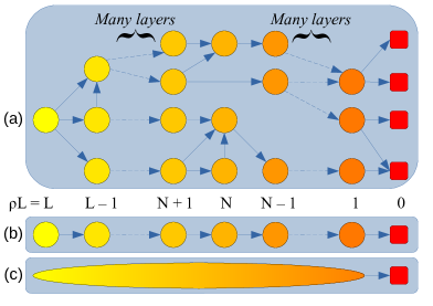
Figure 4: (Color online) (a) Schematic representation of the open (discs) and closed (squares) communicating classes (CCs) and possible transitions between them. The CCs are arranged in decreasing order of their order parameter value $\rho L.$ (b) and (c) represent CCs for $b=0$ and $b\neq 0$ cases of the BDD model respectively.

In summary, we introduce and study a class of birth-death diffusion models where the time-scale of birth and death rates are well separated from the diffusion rate. These models exhibit ordinary and absorbing phase transitions with universal critical lines that do not depend on the nature of diffusion (conserved) dynamics. In the absence of birth, the QSS measure of these systems become nonunique, leading to a novel APT with initial condition-dependent critical exponents. Usually, the origin of varying critical exponents is existence of an underlying marginal operator, which does not scale under renormalization. It is impossible to extend these ideas to include the dependence of critical exponents on initial conditions! In this letter we provide sufficient criteria: A nonunique QSS is possible when the system has multiple open communicating classes, and the transition rates between them have a thermodynamically stable minimum at some nonzero value of the order parameter. More theoretical understanding is required to design or access such nonunique QSSs in experiments.

References

- [1] N.G. Van Kampen, Stochastic Processes in Physics and Chemistry, North Holland (2007).
- [2] D.T. Gillespie, Markov Processes, Academic Press, San Diego (1992).
- [3] R. J. Baxter, Exactly Solved Models in Statistical Mechanics, Academic Press (1982).
- [4] S. Friedli and Y. Velenik,Statistical Mechanics of Lattice Systems: A Concrete Mathematical Introduction, Cambridge University Press (2017).
- [5] D. A. Lavis, Equilibrium Statistical Mechanics of Lattice Models, Springer, Dordrecht (2015).
- [6] C. Vanderzande, Lattice Models of Polymers, Cambridge University Press (1998).
- [7] A. Manacorda, Lattice Models for Fluctuating Hydrodynamics in Granular and Active Matter, Springer Thesis, Rome (2018).
- [8] A. Schadschneider, D. Chowdhury, and K. Nishinari, Stochastic Transport in Complex Systems, Oxford Elsevier (2010).
- [9] S. Abeln, M. Vendruscolo, C. M. Dobson,D. Frenke, PLoS ONE 9, e85185 (2014).
- [10] V. Privman (Ed.), Nonequilibrium Statistical Mechanics in One Dimension, Cambridge University Press (1997).
- [11] M. Henkel, H. Hinrichsen, S. Lübeck, Non-Equilibrium Phase Transitions, Springer, Dordrecht (2010).
- [12] J. Marro and R. Dickman, Nonequilibrium Phase Transitions in Lattice Models, Cambridge University Press (1999).
- [13] T. E. Harris, Contact interactions on a lattice, Ann. Prob. 2, 969 (1974).
- [14] W. Kinzel, Percolation structures and processes, in Ann. Isr. Phys. Soc., edited by G. Deutscher, R. Zallen, and J. Adler, volume 5, Adam Hilger, Bristol, 1983.
- [15] H. Hinrichsen, Adv.Phys. 49, 815 (2000).
- [16] I. Jensen, Critical behavior of the pair contact process, Phys. Rev. Lett. 70, 1465–1468 (1993).
- [17] R. Dickman, M. A. Muñoz, A. Vespinani, and S. Zapperi,Braz. J. Phys. 30, 27(2000).
- [18] M. Basu, U. Basu, S. Bondyopadhyay, P. K. Mohanty, H. Hinrichsen Phys. Rev. Lett. 109, 015702 (2012).
- [19] P. Grassberger, D. Dhar, P. K. Mohanty, Phys. Rev. E 94, 042314 (2016)
- [20] K. A. Takeuchi, M. uroda, H. Chaté, and M Sano, Phys. Rev. Lett. 99 234503 (2007).
- [21] K. A. Takeuchi, M. Kuroda, H. Chaté, and M Sano, Phys. Rev. E80 051116 (2009).
- [22] M. M. de Oliveira and R. Dickman, Phys. Rev. E 71, 016129 (2005).
- [23] R. Wong, Asymptotic Approximations of Integrals. Academic Press Inc., Boston-New York (1989).
- [24] Suzuki, M. New universality of critical exponents. Prog. Theor. Phys. 51, 1992–1993 (1974).
- [25] P.A. Pearce and D Kim, J. Phys. A: Math. Gen. 20, 6471 (1987).
- [26] A. Malakis, A. N. Berker, I. A. Hadjiagapiou, and N. G. Fytas, Phys. Rev. E 79, 011125 (2009).
- [27] J. D. Noh. and H. Park, Phys. Rev. E 69, 016122 (2004).
- [28] N. Khan, P. Sarkar, A. Midya, P. Mandal, P. K. Mohanty, Sc. Reports 7, 1 (2017).
- [29] J. Keizer, On the solutions and the steady states of a Master Equations, J. Stat. Phys. 6, 67-72 (1972).