Electric field measurements on the INCA discharge

Abstract

Developing large-area inductively coupled plasma sources requires deviation from the standard coil concepts and the development of advanced antenna designs. First steps in this direction employ periodic array structures. A recent example is the Inductively Coupled Array (INCA) discharge, where use is made of the collisionless electron heating in the electric field of a periodic array of vortex field. Naturally, the efficiency of such discharges depends on the how well the experimental array realizes the theoretically prescribed field design.

In this work two diagnostic methods are employed to measure the field structure of the INCA discharge. Ex situ B-dot probe measurements are compared to in situ radio-frequency modulation spectroscopy (RFMOS) and good agreement between their results is observed. Both diagnostics show systematic deviations of the experimentally generated field structure from the one employed in the theoretical description of the INCA discharge. The subtleties in applying both diagnostic methods together with an analysis of the possible consequences of the non-ideal electric field configuration and ways to improve it are discussed.

I Introduction

Operation of large area inductively coupled (ICP) discharges at low pressures ($p\leq$100\text{\,}\mathrm{Pa}$$) is very important for various applications [1, 2, 3], because these discharges can provide large ion fluxes needed for anisotropic (directional) surface treatment. However, standard ICP discharges are not ideally suited for providing a homogeneous plasma over large areas ($\sim$1\text{\,}{\mathrm{m}}^{2}$$) at low pressures. An approach to achieve this is to choose an antenna configuration different to the standard flat spiral coil. Several other designs have been developed over the years. The most common alternatives are probably solenoid or dome-shaped antennas [2, 3, 4]. Also some concepts using multiple antennas have been proposed. One of the more recent developments is to replace the coils by linear rods [5, 6, 7]. Apparently, this allows for easy up scaling. However, rather high currents are required to compensate for the comparably low electric field produced by a linear rod.

Recently another possibility was investigated. It is based on a theoretical concept for collisionless resonant electron heating proposed by Czarnetzki and Tarnev [8]. Under collisionless conditions (low pressure) an infinite array of electric RF vortex fields each a distance $L$ apart and oscillating at the frequency $\omega_{0}$ can couple energy efficiently to the electrons. A two-dimensional array of small planar spiral coils realizes such a structure. When the RF current through the coils has the same phase, the structure of the field repeats itself after a distance $\Lambda=L$. The electrons moving at a velocity of $v_{\text{p}}=\Lambda\omega_{0}/2\pi$ parallel to the plane of the array see a constant electric field and are accelerated constantly. Because of the vortex structure of those fields, these electrons never run out of resonance.

This concept was experimentally realized as the INductively Coupled Array (INCA) discharge. It shows consistently a reliable and efficient operation at pressures as low as $0.1\text{\,}\mathrm{Pa}$ [9, 10]. This work was accompanied by a more in-depth theoretical analysis of this electron heating mechanism [11]. It revealed, that the efficient operation is caused by the fact, that all electrons participate in the heating process, making it more efficient than the stochastic heating in standard ICP discharges. By including also the electron collisions with the background gas the theory reveals that for low pressures the collisionless non-local heating prevails and at higher pressures the standard local Ohmic heating dominates [11]. At the pressure for which the mean free path of the electrons $\lambda$ is comparable to the characteristic length of the array $\Lambda$: $\lambda\sim 0.1\Lambda$, the transition between the two regimes occurs [11]. Additionally to the electric field configuration already described, called the ortho-array, another field configuration was proposed and discussed in the theoretical works on the INCA discharge – the so called para-array, where the phase of the current changes by $180\text{\,}\mathrm{\SIUnitSymbolDegree}$ between the neighboring coils [8]. Recently, also this field structure was realized experimentally and it was shown its behavior is very similar to that of the ortho-array [12]. The differences are in good agreement to the theoretical predictions.

In the INCA discharge, the exact local structure of the electric field is vital for its operation in the stochastic mode. In the theoretical works, ideal circular coils where assumed, which produce a purely vortex electric field. However, the practical realization of such coils is not possible, especially for for small coils where the in- and out-connections already lead to a notable deviation of the induced field. Additionally the coils used in the experiments are spiral ones, because they have two windings to enhance the electric field. Till now the structure of the electric field produced by the coils used in the experiment where unknown. In this work, the structure of the electric field is obtained using two different diagnostics. In-situ measurements with RF-modulation spectroscopy (RFMOS) are compared to B-dot measurements (without plasma). The RFMOS measurements also allow an insight into the spatially resolved strength of the residual capacitive coupling in the discharge.

The paper is organized as follows: first the theoretical background of both diagnostics is described and the experimental setup is shown. In section IV the numerical evaluation scheme for the B-dot measurements is outlined. Then the experimental results are shown and both diagnostics are compared in section V. The conclusions with final remarks and an outlook follow in section VI.

II Theory

II.1 RF modulation spectroscopy (RFMOS)

To obtain in situ information about the amplitude and the phase of the induced electric field as well as information about the strength of the capacitive coupling compared to the inductive coupling into the plasma an optical diagnostic called radio frequency modulation spectroscopy (short: RFMOS) is used [13, 14, 15]. For this diagnostic the temporal modulation of the emission from a chosen line (from now on called modulation) is measured using an ICCD camera.

For the further analysis a derived quantity is used, the normalized time dependent modulation $\eta(t)$ during one RF period. It is defined by the ratio of the emission intensity $I(t)$ to its value averaged over one RF period:

$$\eta(t)=\frac{I(t)}{\langle I(t)\rangle}-1.$$ (1)

By using the normalized modulation: the influence of many effects on the measurement is eliminated: camera adjustments (exposure time, gain), background light and inhomogeneity of the electron and the neutral gas density. With the RFMOS technique information about the plasma is obtained from the amplitude and the phase of the different Fourier components of $\eta(t)$. However, the DC component of $\eta(t)$ is always zero due to its definition.

The temporal modulation of the emission intensity arises due to the following reason. In a radio frequency discharge, the time dependent electric field modulates the EEDF, which in turn modulates the excitation to a higher atomic state with excitation energy $\epsilon_{\text{exc}}$ and lifetime $\tau$. When the population of an excited state is modulated, consequently also the spontaneous emission from that state is modulated. This is the fact used by the RFMOS diagnostic technique. This modulation happens mainly at two frequencies: At the first harmonic of the applied RF frequency $\omega_{\text{RF}}$, due to the fact, that the antenna acts as an electrode and there is some capacitive coupling. And at the second harmonic due to the inductive coupling. Because of this, the modulation of the emission intensity in an inductively coupled discharge should be mainly sinusoidal, but can contain some deviations caused by residual capacitive coupling. To separate the components of the modulation at the different frequencies, a Fourier analysis of $\eta(t)$ is performed: $\mathcal{F}_{n\omega}[\eta(t)]=\hat{\eta}_{n\omega}$, where $n$ gives the number of the harmonic of the fundamental frequency. Here this is the frequency of the applied RF signal $\omega_{\text{RF}}$.

To obtain a relation between the intensity modulation $\hat{\eta}_{n\omega}$ and the electric field the following approach is applied. The rate equation for the excited state is combined with the assumption of a time independent, isotropic near Maxwellian distribution of the electrons that is displaced by a small, time dependent oscillation velocity [13, 14, 15]. From this, the measured modulation $\hat{\eta}_{(1,2)\omega}$ can be expressed as follows:

$$|\hat{\eta}_{1\omega}| =\frac{1}{\sqrt{1+{(\omega\tau)}^{2}}}\left(\frac{4}{3}\frac{\epsilon_{\text{exc}}}{k_{B}T_{e}}-2\right)\frac{\vec{u}_{d}\cdot\vec{u}_{\text{osc}}}{v_{\text{th}}^{2}}$$ (2)

$$|\hat{\eta}_{2\omega}| =\frac{1}{\sqrt{1+{(2\omega\tau)}^{2}}}\left(\frac{1}{3}\frac{\epsilon_{\text{exc}}}{k_{B}T_{e}}-\frac{1}{2}\right)\frac{\vec{u}_{\text{osc}}^{2}}{v_{\text{th}}^{2}}$$ (3)

where $v_{\text{th}}$ is the thermal velocity of the electrons and $\vec{u}_{d}$ their DC drift velocity.

Under locality conditions the oscillation velocity $u_{\text{osc}}$ is determined by the local induced electric field:

$$u_{\text{osc}} =\frac{eE}{m_{e}\sqrt{\omega_{\text{RF}}^{2}+\nu_{\text{m}}^{2}}}$$ (4)

with $\nu_{\text{m}}$ the electron collision frequency. Due to this relation, the amplitude of the second harmonic of the modulation ($\hat{\eta}_{2\omega}$) is proportional to the square of the induced electric field.

Usually the amplitude of the modulation is weak (a few percent). In an inductively coupled discharge, it is even smaller compared to capacitive discharges [16]. To measure the small change in the plasma emission, the detector must be very sensitive and the spectral line used should be chosen carefully. The upper state of the observed transition should not be populated from metastable states or by cascades, i.e. it has to be populated predominantly from the ground state. This requirement is specially important, because the excitation from the ground state to a high state is mainly determined by the high energetic tail of the EEDF. This part of the distribution function also is the one that is most affected by the variation of the induced electric field. Due to this, the modulation of the emission from such a highly energetic state is stronger compared to the one from a low energy state. This can also be seen in the equations (eqs. 2 and 3), the amplitudes of the first and second harmonic increases with the excitation energy $\epsilon_{\text{exc}}$. The other requirement is, that the lifetime of the excited state should be much shorter than the RF period ($\tau_{\text{rf}}=$74\text{\,}\mathrm{ns}$$), so that no averaging over time happens. This is also seen in eqs. 2 and 3, where the amplitude decreases for increasing values of $\tau$. For the measurements in hydrogen performed in this work, the H_α line is used [15].

II.2 B-dot measurement

To determine the electrical field of a coil or an arrangement of coils first the magnetic field is measured. This is done by inserting a conductive loop oriented towards $\hat{e}_{i}$ into the field and measuring the induced voltage. In the following only fields produced by flat coils in the x-y-plane are considered.

The voltage $U_{\text{ind}}$ induced by a time dependent magnetic flux $\phi$ into the conductive loop is given by Faraday’s law:

$$U_{\text{ind}} =-\frac{\mathrm{d}\phi}{\mathrm{d}t}=-\frac{\mathrm{d}}{\mathrm{d}t}\int\vec{B}\cdot\mathrm{d}\vec{S}$$ (5)

Here $\vec{B}$ is the magnetic field, $\vec{S}=S\vec{n}$ with $S$ the area of the conductive loop and $\vec{n}$ the normal vector of its area. If the conductive loop is oriented towards $\hat{e}_{i}$ and has $N$ windings:

$$U_{\text{ind}} =-N\frac{\mathrm{d}}{\mathrm{d}t}B_{i}S$$ (6)

where $B_{i}$ is the $i$ component of the mean magnetic field inside the conductive loop. When the loop is stationary and the magnetic field is harmonic in time ($B\propto e^{i\omega t}$) it follows

$$B_{i} =-\frac{U_{\text{ind}}}{i\omega NS}$$ (7)

To measure the full magnetic field this measurement must be preformed separately three times, once with the loop oriented towards each coordinate axis.

To calculate the electric field $\vec{E}$ from the measured magnetic field, there are in principle two options: Using the curl of the magnetic field or using the rotation of the electric field. While the first one seems to be the superior one, because it assumes no knowledge about the form of the electric field, it has some numerical difficulties. Assuming also the electrical field to be harmonic, from the curl of $\vec{B}$ follows: $\vec{E}=c^{2}/(i\omega)\nabla\times\vec{B}$. In the curl there small differences of rather large quantities are calculated and that is numerically unstable. Because of this, the curl of the electric field Ansatz is promising. However, here one assumption is needed: $E_{z}=0$, this approximation if fine, because the coils are in the x-y-plane and thereby there are no currents in z-directions, which could cause electric fields in z-direction. Assuming that also $E_{x},E_{y}$ vanish at $z\to\infty$ it follows

$$E_{x} =-i\omega\int_{\infty}^{z}B_{y}\mathrm{d}z$$ (8)

$$E_{y} =i\omega\int_{\infty}^{z}B_{x}\mathrm{d}z$$ (9)

The consistency of the measured magnetic field would normally be checked by using $\nabla\cdot\vec{B}\overset{!}{=}0$. But in this calculation again small differences of large quantities appear, so it is numerically unstable. Nevertheless, every curl-field is divergence free, so it is sufficient to test for $\nabla\times\vec{E}=-i\omega\vec{B}$. The $x$- and $y$-component of this equation were already used to calculate the electric field, so that it is sufficient to check the $z$-component:

$$\partial_{x}E_{y}-\partial_{y}E_{x} \overset{!}{=}-i\omega B_{z}$$ (10)

Here $B_{z}$ is calculated from $E_{x,y}$ and than compared to the independently measured $B_{z}$ field. If both are the same, the divergence of the magnetic field vanishes and the diagnostic is consistent. However, this does not test the assumption of $E_{z}=0$, because the contributions of _z to the derivatives of $E_{x,y}$ cancel out.

III Experimental Setup

III.1 Discharge Setup

A more detailed description of the discharge setup can be found elsewhere [9, 10]. Here only a brief description is give. The INCA discharge consists of a rectangular stainless steel vacuum chamber ($40\text{\times}40\text{\times}25.6\text{\,}\mathrm{cm}$). The antenna array is positioned roughly in the middle of the short side, dividing the volume into two separate regions. On one side (depth $13\text{\,}\mathrm{cm}$) the plasma is created by supplying a $13.56\text{\,}\mathrm{MHz}$ RF signal through an L-type matching box to the antenna. After the matching box, but before the vacuum feedthrough the current is measured. The power is produced by a Dressler Cesar generator. The other side houses the wiring and the cooling of the antenna array. The placement of the array inside the vacuum chamber is to avoid mechanical stress due to pressure difference over its large area ($40\text{\times}40\text{\,}\mathrm{cm}$).

The antenna array consists of $6\text{\times}6$ flat spiral coils, with two windings each and a thickness of $3\text{\,}\mathrm{mm}$. The coils are made of copper and occupy an area of $5\text{\times}5\text{\,}\mathrm{cm}$, i.e. $L=$5\text{\,}\mathrm{cm}$$. The individual coils are connected with each other through copper stripes. The previous studies [9, 10] have shown that for a matching to be possible, the coil wiring has to be separated into three parallel branches, each containing $12$ coils connected in series.

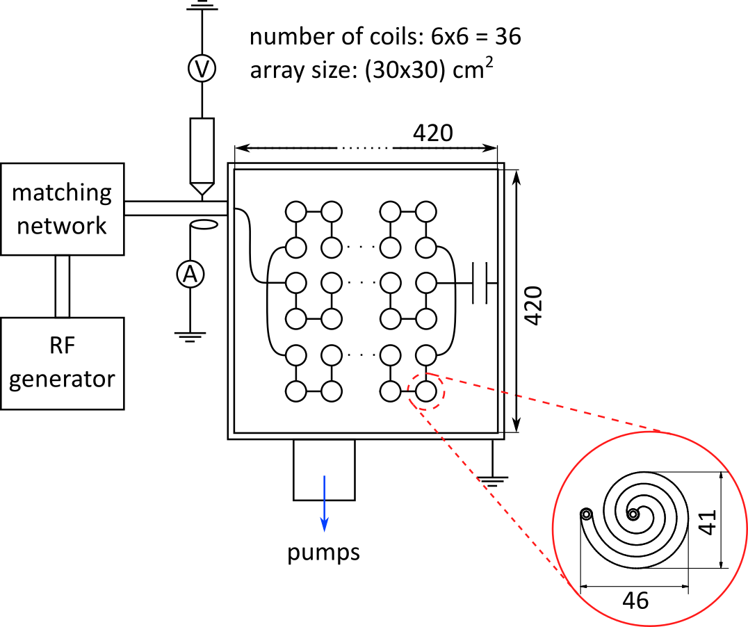
Figure 1: Schematics of the discharge chamber, the dimensions are given in mm.

The temporally and spatially resolved emission from the plasma is measured using an ICCD camera (HR16-PicoStar, LaVision) which is placed in front of the antenna facing lid of the discharge chamber. The antenna facing lid has three windows aligned on the diagonal of it. In this work mainly the central window and seldom the upper right window are used.

III.2 B-dot probe system setup

The homemade B-dot probe consists of a copper rod containing two wires fig. 2. At the end of the rod a connector for a pick-up coil is installed. For the measurement of the $x$- and the $y$-component of the magnetic field, the same pick-up coil is used, only the rod is rotated. For the $z$-component a similar coil with different orientation is used. The pick-up coils are made of copper wire, each have a diameter of $5\text{\,}\mathrm{mm}$ and $5$ windings. To measure the magnetic field not only in one point, but on a grid, the probe is mounded on a three-axis movement table. Its movement in the $xy$- plane is controlled by two stepper motors and its movement along the $z$-axis is controlled manually. The maximum measurement area is $90\text{\,}\mathrm{mm}$ in $x$-, $200\text{\,}\mathrm{mm}$ in $y$- and $100\text{\,}\mathrm{mm}$ in $z$-direction.

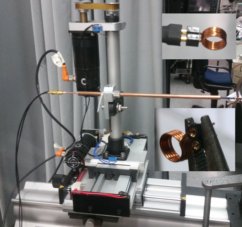
Figure 2: Photograph of the homemade B-dot probe system with enlarged inlets of the pick-up coils for the $x$- and $y$- component of the $B$-field (top) and for the $z$-component (bottom).

The ends of the pick-up coil are connected to an oscilloscope (LeCroy wavepro 7100A) using separate coaxial cables. For triggering and comparison also the current measurement of the chamber is connected to the oscilloscope. To determine the induced voltage in the pick-up coil, the difference of the voltages at both ends of the coil is determined on the oscilloscope. High-frequency noise is suppressed by using an internal $20\text{\,}\mathrm{MHz}$ filter on all channels. Because the induced voltage is a harmonic oscillation with a known frequency only its amplitude and its phase are recorded (see following section). Fluctuations in the generator power are accounted for by recording also the amplitude of the current through the antenna.

The measurement is controlled by two self-written programs running on the oscilloscope. The main program controls the measurement and the movement of the stepper motors. For the recording itself, the second program is called that controls the oscilloscope. It records all quantities averaged over $1\text{\,}\mathrm{s}$. For the movement a 3D scan is implemented, that scans each $x$-, $y$-plane in a serpentine pattern and instructs the user to set the $z$-position accordingly after scanning each plane. In this work, a grid size of $5\text{\,}\mathrm{mm}$ in each direction was used, because this is also the size of the pick-up coils which effectively limits the maximum spatial resolution.

IV Data evaluation

In the numerical evaluation of the induced voltage to determine the magnetic field, also the phase of the induced voltage must be considered. The equation for a harmonic wave $G$ with a positive amplitude $A(\vec{r})$, wave number $\vec{k}$ and frequency $\omega$ at time $t$ and position $\vec{r}$ is

$$G(\vec{r},t)=A(\vec{r})\exp\left\{i\left(\omega t-\vec{k}\cdot\vec{r}+\varphi_{0}+\varphi_{\text{sgn}}(\vec{r})\right)\right\}$$ (11)

Here $\varphi_{0}$ is an unknown but constant initial phase and $\varphi_{\text{sgn}}(\vec{r})=\{0,\pi\}$ describes the sign of the field at the position $\vec{r}$. The time dependence was not recorded, so that the measured phase is

$$\Delta\varphi(\vec{r}) =-\vec{k}\cdot\vec{r}+\varphi_{0}+\varphi_{\text{sgn}}(\vec{r}).$$ (12)

The initial phase may be chosen arbitrarily, here we use $\varphi_{0}=0$. The magnitude part of the equation can be estimated: $\left|\vec{k}\cdot\vec{r}\right|=2\pi r/\lambda$. For a frequency of $13.56\text{\,}\mathrm{MHz}$ the wavelength is $\lambda\approx$22\text{\,}\mathrm{m}$$ and all distances in the experiment are smaller than $20\text{\,}\mathrm{cm}$ and the influence of this part can be neglected. Because of this, the measured phase contains only the sign of the field. Because of this, it is necessary to extract the sign from the phase, which is involved, because the numerical values of the phases contain uncertainties. This is done for each x-y-plane and each Cartesian component separately. For every plane a histogram of all phases measured is created (see fig. 3 for an example of such a histogram). In the histogram the highest and the second highest peaks are found. These peaks should be about $180\text{\,}\mathrm{\SIUnitSymbolDegree}$ apart and build the most likely phases for both signs. Now the phase is shifted, so that the peak at a higher angle is at $90\text{\,}\mathrm{\SIUnitSymbolDegree}$. By this the peaks should be near $+$90\text{\,}\mathrm{\SIUnitSymbolDegree}$$ and $-$90\text{\,}\mathrm{\SIUnitSymbolDegree}$$ and the number of measurements where the phase is near zero should be minimal. The next step is to get the sign of the shifted phases as a first approximation of the field’s sign. However, because of statistical fluctuations and external distortions, there are still single points, where the field is weak and the distortions were large enough to determine the wrong sign. To correct for this use is made of the fact that it is not physical to have single points with a phase that is significantly different from that of all surrounding points. Because of this, the sign of all points, that have a different sign than their x- and y-neighbors, is changed. This correction is not applied at the edge of the measurement area. Knowing the sign of the magnetic field components, eq. 7 is used to determine also the amplitude of the field components.

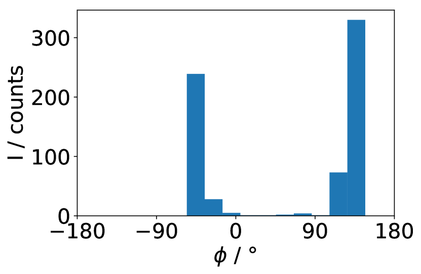
Figure 3: Example of a histogram of all phases of the induced voltage measured in one x-y-plane.

The second part of the data evaluation is to calculate the electric field from the magnetic field. This calculation is done via the curl of the electric field (see eqs. 8 and 9). For this calculation $B_{x}$ or $B_{y}$ must be integrated with respect to $z$. Numerically this is realized using the Riemann sum

$$\int_{\infty}^{z_{i}}G(z^{\prime})\mathrm{d}z^{\prime}=\Delta z\sum_{j=i}^{N}G_{j}$$ (13)

where $G_{j}$ is the value of $G$ at $z_{j}=z_{0}+j\Delta z$. The obvious advantage of this method is that the electric field can be calculated for all points where the magnetic field is known.

To get the calculated z-component of the magnetic field the numerical derivatives of $E_{x,y}$ are needed. Therefore, the symmetric difference quotient is used

$$f^{\prime}(x)\approx\frac{f(x+\Delta x)-f(x-\Delta x)}{2\Delta x}.$$ (14)

Its advantage is that in this way the derivatives are calculated at the grid points of the function and these grid points are the same for the measured magnetic field. The disadvantage of it is that the derivatives can not be calculated at the edge of the measurement area.

V Results

In fig. 4 the magnetic field of a part of the INCA antenna array is shown. It was measured using the B-dot probe directly in front of the quartz window. In all three field components the individual coils are clearly visible and nearly no asymmetry occurs. As one can expect, the $z$-component of the field is much stronger than the $x$- and $y$-components. This is because the current through the antenna array is mainly a circulating current and only a small part of the current is in radial direction. This radial current is caused by the radius change of the spiral coils. If the coils would be ideal circular ones, there would be no current component in radial direction.

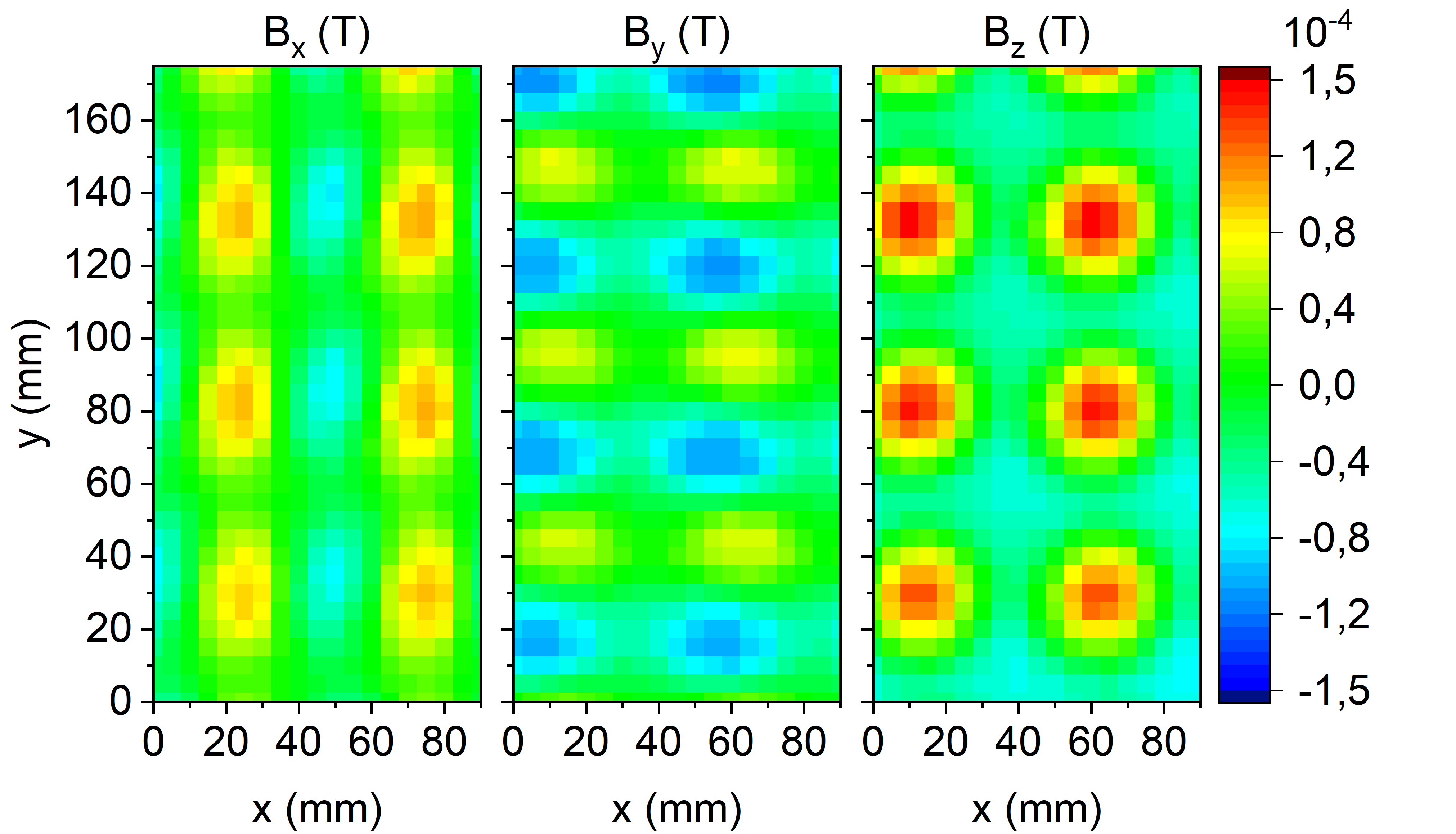
Figure 4: Magnetic field of a part of the INCA antenna array, measured with the B-dot probe directly in front of the quartz window.

In the theory section (section II), a procedure was shown to check the consistency of the B-dot measurements and specially the numerical calculation of the electric field. The calculated and the measured magnetic field have a very similar structure. However, the normalized difference shows rather strong deviations in the proximity of the coil’s edges. The reason for those deviations is apparent: They are at the positions where the spatial dependence of the electric field components is high. In calculating the $z$-component of the magnetic field from the electric field components (eq. 10) the difference of the spatial derivatives of $E_{x,y}$ is calculated. Here, it is a small difference of large numerical quantities, so the numerical error is high.

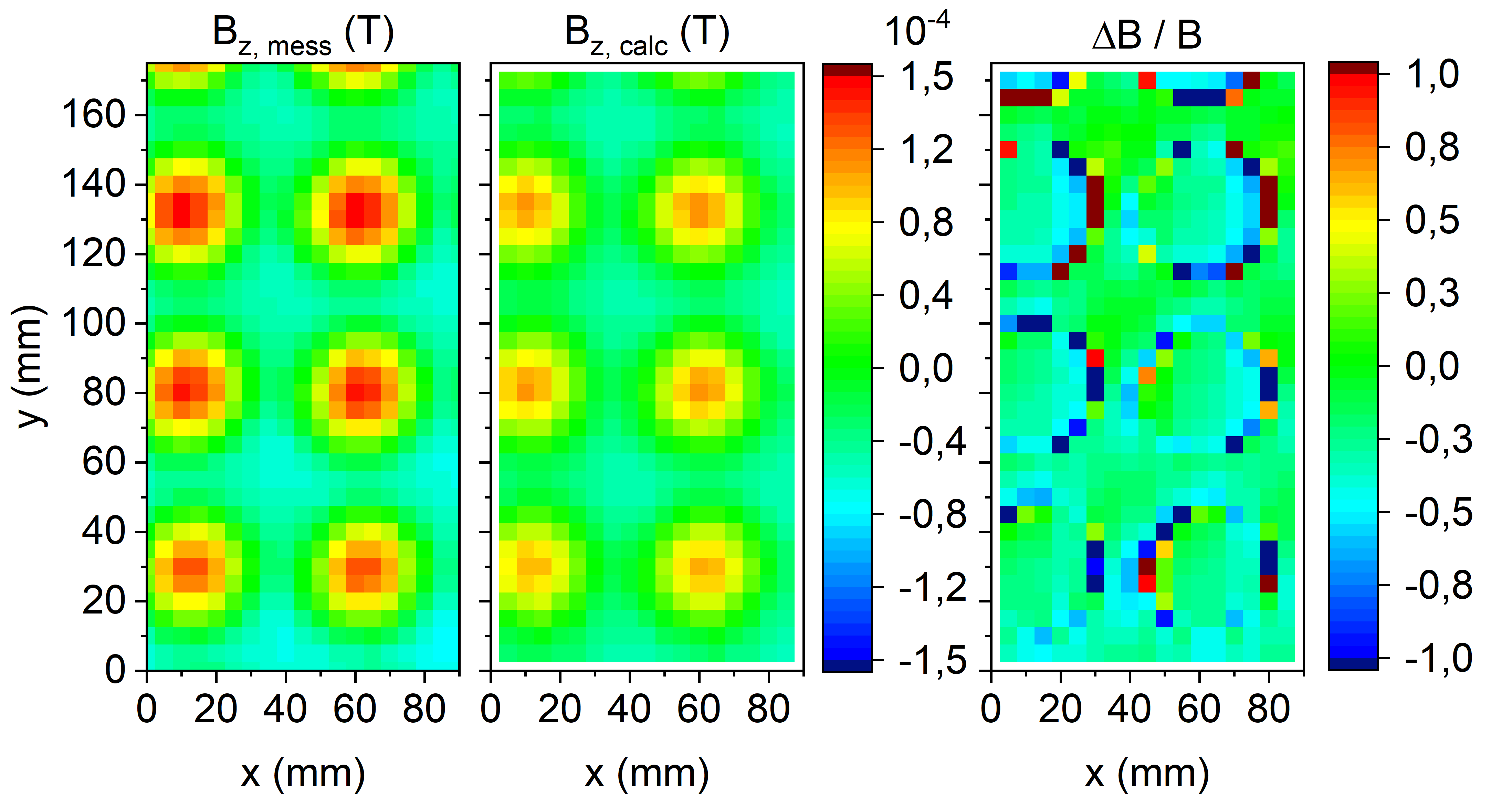
Figure 5: Comparison between directly measured ($B_{z,\text{mess}}$) and from the electric field calculated ($B_{z,\text{calc}}$) $z$-component of the magnetic field of a part of the INCA antenna array obtained using the B-dot probe. Additionally the relative difference is shown.

The deviations outside of coil edge regions are small and do not show any structure. There are various reasons, that also there the difference does not vanish completely. This comparison combines three individual measurements. Variations of the generator output were compensated by using the current through the antenna array as a reference, but this might not eliminate all variations. Also, a different pick-up coil is used for measuring the $z$-component of the magnetic field. As one can see in fig. 2 the position of this pick-up coil relative to the holder is slightly different. Due to this difference in the measurement girds of the different components of the magnetic field, deviations between the measured and the calculated $z$-component of the magnetic field might occur. Because the differences are still small, the consistency of the diagnostic is confirmed by this comparison.

The quantity that is more important for the operation of the INCA discharge is the square of the electric field [11]. Having confirmed, that the B-dot diagnostic is consistent, it provides ex situ (without plasma) access to the structure of the electric field. The measured square of the electric field in the direct proximity of the quartz window using the B-dot probe is shown in fig. 6. In this figure the red circle marks the region, that is also accessible to the RFMOS diagnostics at the central window.

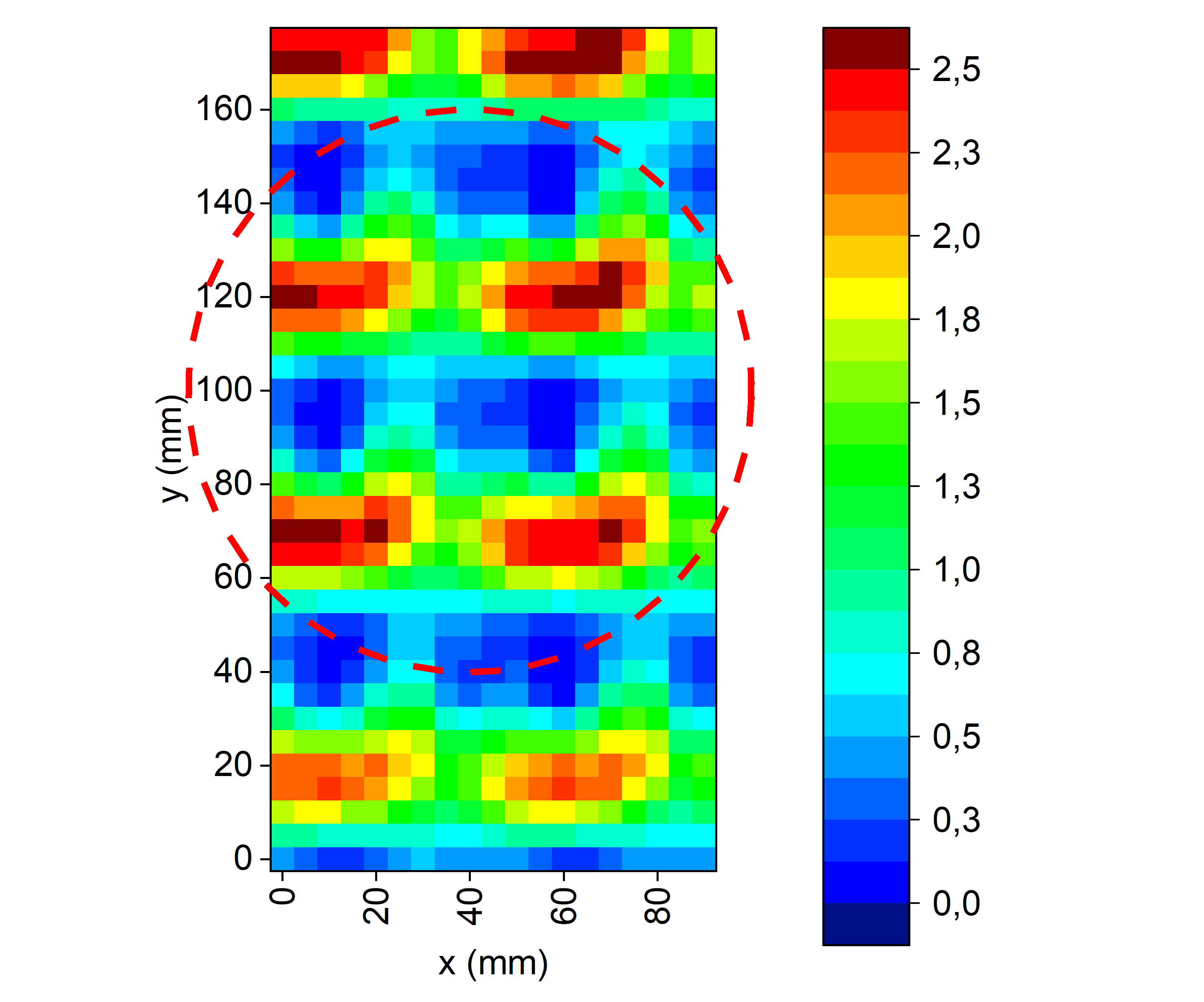
Figure 6: Structure of the square of the induced electric field, $E^{2}$, from the antenna obtained using the B-dot probe. The red circle marks the region, that is also accessible to the RFMOS diagnostic at the central window.

The structure of $E^{2}$ is far from the one created by ideal circular coils, which was assumed in the theoretical investigations of the INCA discharge [11, 8]. Instead the field is strongly asymmetric and shows kidney-like structures. It is also apparent, that the different coils influence each other as the intensity of the “kidneys” varies rather strongly between the individual coils.

Using the RFMOS diagnostics it is also possible to measure the square of the electric field in situ. However, it is important to take the locality of the electrons into account when interpreting the RFMOS measurements. At higher pressures, where all electrons are local, from the modulation at one point, the induced electric field at that point can be obtained. At lower pressure, the electrons become non-local and the modulation at one point is also influenced by the field at other positions, so that the result smears out spatially.

To be sure, that the electrons are all local, a measurement is performed at $15\text{\,}\mathrm{Pa}$ and $600\text{\,}\mathrm{W}$ in hydrogen. At these conditions, the mean free path of the electrons is few millimeters [1]. The modulation of the H_α line was recorded with an ICCD camera through the middle front window. From this position the central region of $2\times 2$ coils is visible. The second harmonic of the modulation is proportional to $u_{\text{osc}}^{2}$, i.e. the square of the induced electric field, $E^{2}$ (see eq. 3), and is shown together with its phase in fig. 7. The figure also shows the values from the B-dot measurements (fig. 6). The agreement between the two independent diagnostics is very good. The modulation of the top left coil is relatively weak, but this could be an optical artifact. The phase of the second harmonic (see fig. 7) is relatively homogeneous and shows no structure. This is not surprising as these four coils are all connected in series. Therefore, the current and the induced electric field are in phase.

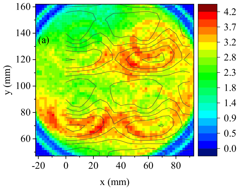
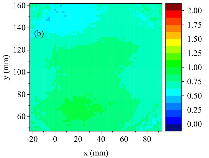
Figure 7: 7 Amplitude and 7 phase of the second harmonic of the temporal modulation of the H_α line in a hydrogen plasma at $15\text{\,}\mathrm{Pa}$ and $700\text{\,}\mathrm{W}$. The color plots show the modulation in percent and the phase in units of $\pi$, respectively. The contour lines on the amplitude plot represent $E^{2}$ from the B-dot measurements. The coordinate system is the same as for the B-dot measurements (fig. 6).

To confirm that the measurement works as intended and the spatial structures in the second harmonic of the modulation disappear at lower pressures, a measurement at $0.8\text{\,}\mathrm{Pa}$ and $700\text{\,}\mathrm{W}$ in hydrogen was performed. The second harmonic from that measurement is shown in fig. 8. As expected, nearly no structure remains.

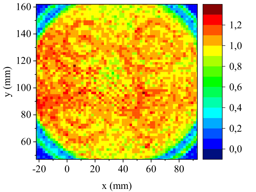
Figure 8: Amplitude of the second harmonic of the temporal modulation of the H_α emission in a hydrogen plasma at $0.8\text{\,}\mathrm{Pa}$ and $700\text{\,}\mathrm{W}$. The colors represent the amplitude in percent.

The amplitude and phase of the first harmonic of the modulation are a measure of the scalar product of drift velocity $\vec{u}_{\text{d}}$ and oscillation velocity $\vec{u}_{\text{osc}}$  (eq. 2). There are two reasons for $\vec{u}_{\text{d}}\cdot\vec{u}_{\text{osc}}$ to be nonzero. The first one is the drift velocity from the ambipolar diffusion in the $xy$-plane and the oscillation velocity in the same plane (due to the inductive coupling). However, this should be zero only in the center and become nonzero everywhere else, because the $u_{\text{amp}}$ is only zero in the center and fig. 7 shows, that the oscillation velocity is nonzero everywhere. The second one is the drift velocity from ambipolar diffusion in the $z$-plane and the oscillation velocity in that plane due to capacitive coupling. A first harmonic caused by this may have any form. The amplitude and phase of the first harmonic of the modulation, again at $15\text{\,}\mathrm{Pa}$ and $700\text{\,}\mathrm{W}$ are shown in fig. 9. There is a vertical line, where the amplitude is zero and the phase has a jump of about $180\text{\,}\mathrm{\SIUnitSymbolDegree}$. This line passes through the center of the discharge. Therefore, it is more likely that the first harmonic here corresponds to the strength of the capacitive coupling.

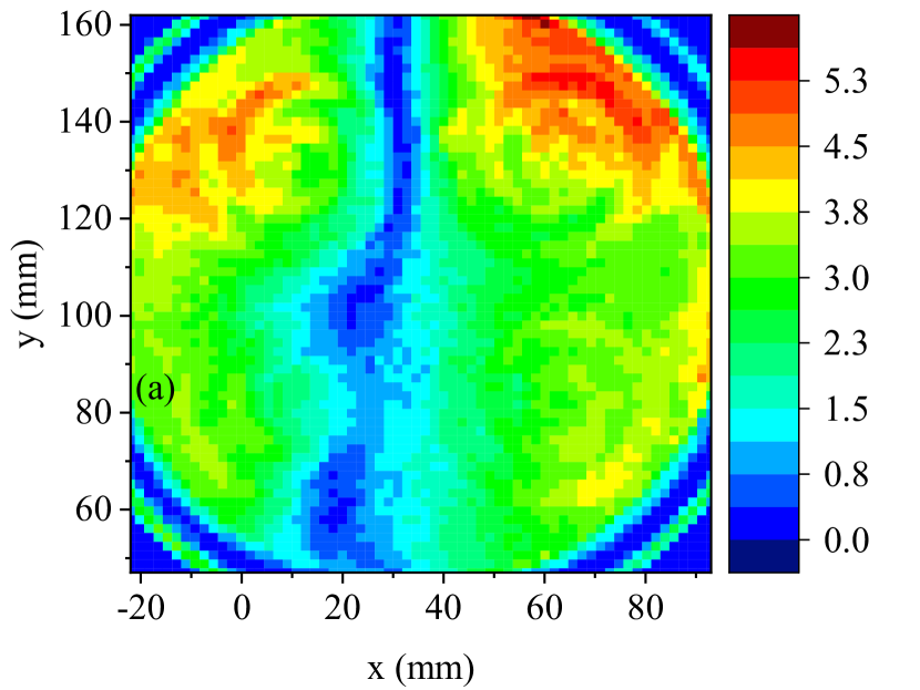
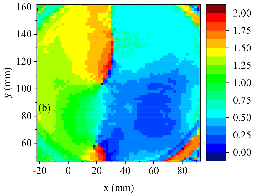
Figure 9: 9 Amplitude and 9 phase of the first harmonic of the H_α emission in a hydrogen plasma at $15\text{\,}\mathrm{Pa}$ and $700\text{\,}\mathrm{W}$. The color plot represents the amplitude in percent and the phase in units of $\pi$, respectively.

Such a spatial dependence of the capacitive coupling in the INCA discharge corresponds to the design of the discharge. An additional capacitor between antenna and ground was added to decrease the capacitive coupling [10]. This adds a virtual ground point in the middle of the three arms of the antenna. At this ground point the RF potential should be approximately zero, so there should be no capacitive coupling. Also there should be a phase jump of $180\text{\,}\mathrm{\SIUnitSymbolDegree}$, because the RF potential changes its sign at that position. This corresponds extremely well with the results from the RFMOS measurement.

To check that the vanishing capacitive coupling only occurs in the (horizontal) center of the discharge another measurement at $15\text{\,}\mathrm{Pa}$ was performed at the upper front window. The amplitude of the first harmonic at that position is shown in fig. 10. Note that the scale of these two figures is not the same. The maximum of the amplitude in the central region is about $5.4\text{\,}\mathrm{\char 37\relax}$, whereas the one in the corner region is significantly higher, up to about $11\text{\,}\mathrm{\char 37\relax}$. The structure of the first harmonic measured in the corner of the discharge supports the previous considerations. Here the amplitude of the first harmonic is much stronger, no line of zero capacitive coupling is visible and the coils form the maximum. All this indicates that the capacitive coupling of the INCA discharge is consistent with its design.

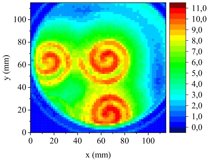
Figure 10: Amplitude of the first harmonic of the temporal modulation of the H_α line in a hydrogen plasma at $15\text{\,}\mathrm{Pa}$ and $700\text{\,}\mathrm{W}$ measured through the upper front window. The color plot represents the amplitude in percent.

This also points out another property of the INCA discharge. Due to the virtual ground point in the horizontal center of the antenna, the highest voltage does not occur in the center of the discharge but at the left and right side of it, which increases the capacitive coupling there. Also the electron density is low there, because of the diffusion profile [9], which again enhances the capacitive coupling. This is another possible explanation for the surprisingly high plasma potential, which was attributed to an overpopulation of highly energetic electrons [9]. To confirm one or the other theory it would be necessary to measure the density of electrons overcoming the sheath potential at least quantitatively.

VI Conclusion

Two different diagnostics were used to measure the electric field structure of the antenna array of the INCA discharge. The more straightforward one, the B-dot probe, provides only ex situ measurements while the other one, the radio frequency modulation spectroscopy, provides directly in situ results. The results from the two diagnostic methods agree very well with each other. A criterion for the consistency of the B-dot measurements was developed and applied to the measurements. The structure of the electric field is far from ideal, hinting to the need of improved coil design that could lead to an improvement of the heating efficiency. Nevertheless, the measured electric field structure is well in line with earlier theoretical estimations [10]. A possible design for more ideal coils could be one, that is still spiral but where the inner diameter is larger. This would require the coils to be slightly narrower, but the stray current in radial direction would also be smaller.

The strength of the capacitive coupling in the INCA discharge was also determined with spatial resolution. It is confirmed that the designated virtual ground point works as intended. This also leads to another explanation for the surprisingly high plasma potential, which could be tested by measuring the density of electrons overcoming the sheath potential.

References

- Lieberman and Lichtenberg [2005] M. A. Lieberman and A. J. Lichtenberg, Principles of Plasma Discharges and Material Processing (JOHN WILEY & SONS INC, 2005).
- Hopwood [1992] J. Hopwood, “Review of inductively coupled plasmas for plasma processing,” Plasma Sources Sci. Technol. 1, 109–116 (1992).
- Okumura [2010] T. Okumura, “Inductively coupled plasma sources and applications,” Physics Research International 2010, 1–14 (2010).
- Godyak and Demidov [2011] V. A. Godyak and V. I. Demidov, “Probe measurements of electron-energy distributions in plasmas: what can we measure and how can we achieve reliable results?” Journal of Physics D: Applied Physics 44, 233001 (2011).
- Guittienne et al. [2017] P. Guittienne, R. Jacquier, A. A. Howling, and I. Furno, “Electromagnetic, complex image model of a large area RF resonant antenna as inductive plasma source,” Plasma Sources Science and Technology 26, 035010 (2017).
- Hollenstein, Guittienne, and Howling [2013] C. Hollenstein, P. Guittienne, and A. A. Howling, “Resonant RF network antennas for large-area and large-volume inductively coupled plasma sources,” Plasma Sources Science and Technology 22, 055021 (2013).
- Lecoultre et al. [2012] S. Lecoultre, P. Guittienne, A. A. Howling, P. Fayet, and C. Hollenstein, “Plasma generation by inductive coupling with a planar resonant RF network antenna,” Journal of Physics D: Applied Physics 45, 082001 (2012).
- Czarnetzki and Tarnev [2014] U. Czarnetzki and K. Tarnev, “Collisionless electron heating in periodic arrays of inductively coupled plasmas,” Phys. Plasmas 21, 123508 (2014).
- Ahr et al. [2018] P. Ahr, T. V. Tsankov, J. Kuhfeld, and U. Czarnetzki, “Inductively coupled array (INCA) discharge,” Plasma Sources Sci. Technol. 27, 105010 (2018).
- Ahr [2018] P. Ahr, Investigation of an efficient stochastic electron heating mechanism in periodically structured vortex fields, Ph.D. thesis (2018).
- Czarnetzki [2018] U. Czarnetzki, “Kinetic model for stochastic heating in the INCA discharge,” Plasma Sources Sci. Technol. 27, 105011 (2018).
- Lütke Stetzkamp, Tsankov, and Czarnetzki [2021] C. Lütke Stetzkamp, T. V. Tsankov, and U. Czarnetzki, “Operation of the inductively coupled array (INCA) discharge as a para-array,” J. Phys. D: Appl. Phys. (2021), 10.1088/1361-6463/ac0c4b.
- Crintea et al. [2008] D. L. Crintea, D. Luggenhölscher, V. A. Kadetov, C. Isenberg, and U. Czarnetzki, “Phase resolved measurement of anisotropic electron velocity distribution functions in a radio-frequency discharge,” J. Phys. D: Appl. Phys. 41, 082003 (2008).
- Celik et al. [2011] Y. Celik, D. L. Crintea, D. Luggenhölscher, U. Czarnetzki, T. Ishijima, and H. Sugai, “Wave propagation and noncollisional heating in neutral loop and helicon discharges,” Phys. Plasmas 18, 022107 (2011).
- Tsankov et al. [2011] T. Tsankov, U. Czarnetzki, Y. Takeiri, and K. Tsumori, “A discharge with a magnetic x-point as a negative hydrogen ion source,” (AIP, 2011).
- Kadetov [2004] V. A. Kadetov, Diagnostics and modeling of an inductively coupled radio frequency discharge in hydrogen, Ph.D. thesis (2004).