Mobile Microphone Array Speech Detection and Localization in Diverse Everyday Environments

Abstract

Joint sound event localization and detection (SELD) is an integral part of developing context awareness into communication interfaces of mobile robots, smartphones, and home assistants. For example, an automatic audio focus for video capture on a mobile phone requires robust detection of relevant acoustic events around the device and their direction. Existing SELD approaches have been evaluated using material produced in controlled indoor environments, or the audio is simulated by mixing isolated sounds to different spatial locations. This paper studies SELD of speech in diverse everyday environments, where the audio corresponds to typical usage scenarios of handheld mobile devices. In order to allow weighting the relative importance of localization vs. detection, we will propose a two-stage hierarchical system, where the first stage is to detect the target events, and the second stage is to localize them.

The proposed method utilizes convolutional recurrent neural network (CRNN) and is evaluated on a database of manually annotated microphone array recordings from various acoustic conditions. The array is embedded in a contemporary mobile phone form factor. The obtained results show good speech detection and localization accuracy of the proposed method in contrast to a non-hierarchical flat classification model.

I Introduction

Sound source localization (SSL) aims to determine either the direction or position of the source in a continuous or discrete-valued space, and automatic sound event detection (SED) aims to recognize the classes of the source sounds present, and estimate their temporal activities. The SSL and SED have been extensively researched mostly as separate problems. Deep learning methods have brought improvements in SSL performance [1, 2, 3, 4, 5, 6, 7, 8, 9, 10] and in SED [11, 12, 13, 14] over traditional approaches. Recent approaches solving simultaneously the SED and SSL problems, i.e., joint sound event detection and localization (SELD) problem, include using Convolutional Neural Networks [15, 16], Convolutional Recurrent Neural Network (CRNN) [17, 18, 19], and the Least Absolute Shrinkage and Selection Operator (LASSO) [20].

As the research in the field has progressed towards machine learning approaches, the data used to train a system has a crucial impact on its performance. Larger and more diverse datasets enable learning more complex models that will generalize better to new conditions. Since recording of acoustic scenes with spatiotemporal annotations is an extremely difficult task, there are no large-scale datasets of real scenes, and existing smaller ones are limited to evaluation of algorithms and are unsuitable for training deep-learning methods (e.g. LOCATA challenge [21]). That is in contrast, e.g., to automatic speech recognition where annotation is not a problem and recorded datasets exist with diverse range of conditions (e.g., the ASpIRE [22] and CHiME [23] challenges). Hence, for deep-learning based SSL researchers have generally relied on either simulations for training and testing on a small recorded dataset [24, 25], or on emulated scenes with real recorded room impulse responses (RIRs). The second option allows integrating real acoustics with source signals of interest with a few RIR datasets available [26, 27, 28]. Additionally, the SELD datasets related to the DCASE challenge have been generated with a large scale RIR collection from 15 rooms and a spherical microphone array [19]. The only annotated dataset for SELD with real recordings we are aware of is the one in [29] for office environments.

In this study, a microphone array embedded inside a flat mobile phone body was used to collect a dataset from diverse everyday environments to obtain insights for realistic mobile phone applications of the SELD approaches. To our knowledge, a microphone array in a mobile phone form factor has not been dealt with in previous SELD research. The flat microphone array shape imposes challenges to the spatial resolution rendering the task more difficult in contrast to, e.g., spherical arrays. Therefore, we do localization using only two categories, front and back, with respect to a mobile phone screen. This is motivated by possible mobile phone multimedia applications. We focus the evaluation on localization and detection of speech and detection of other prominent sounds of interest without localizing them.

State of the art SELD systems typically train a single system for joint localization and detection. In order to allow controlling the relative importance of localization vs. detection, we propose a hierarchical approach of two separate deep neural networks, optimized for their corresponding tasks.

In this paper Section II describes the database collection. Section III describes the proposed hierarchical two-stage SELD approach. Section IV describes the evaluation of the SED, SSL, and the joint system and then compares the results to a baseline classifier. Finally, Section V draws the conclusions and future directions.

II Dataset

TABLE I: Duration (s) of recordings for each environment.

Apartment	1094	Industrial area	920	Club room	630	Studio room	419
Street	404	Meeting room	335	Corridor/office	245	Park	226
Live club	210	Car	185	Urban area	110	Stairs	105
Lake	65	Cycle path	60	Ship’s deck	60	Subway	51
Store room	45	Grocery store	41	Marketplace	40	Beach	20
Harbour	20	Terrace	15	Cafe	15	Terminal	11

Data collection and annotation

Acoustic data for training and evaluation of the methods was collected in complex real-life environments. Actions and objects in the recordings aim to represent typical contents of casual videos recorded by a typical mobile phone user. The data set contains speech and other scene-specific sounds from common scenarios such as sports, moving vehicles and live music. In total there are 24 environment types including both indoor- and outdoor scenes, refer to Table I. The duration of the recordings varies from 10 to 180 seconds, and the total duration is 89 min.

The audio data was collected with an eight-channel microphone array mounted to a custom 3D-printed rigid phone-shaped body. In addition, a 360^∘ camera was used to make the annotation task easier and a web camera was used to collect video material for later research purposes. The devices were fixed to a hand-held microphone stand during the recordings that was was held from a grip below to prevent obstructing sensors. Figure 1 illustrates the recording setup and the microphone array. A laptop was used to collect the eight-channel audio as wav files at 48 kHz sampling rate and 32-bit resolution.

The recorded signals were annotated with the following labels using one-second resolution: (1) Speech back: A person was speaking from behind the microphone array, e.g., the person holding the device. (2) Speech front: A person in front of the array was speaking. (3) Something else: An object was emitting interesting non-speech sound. Multiple labels were allowed to be used simultaneously. The direction for the class ”something else” was not used, since it was not considered as interesting as for the speech. Besides, the direction for this class is often ambiguous and rather hard to annotate.

A sound was considered interesting if the sound source was the focus of the recording or the sound was otherwise special in the context of the environment. For example, a scenario on a beach where a diver jumped into water in front of the array was assigned the label ”Something else” during the time of a splash. Other swimmers talking in the background and creating similar splashing sounds were considered as background, since they were not in a key role from the perspective of the cameraman. Therefore, the boundary between interesting sounds and background noise is inevitably ambiguous, since the same sound can be assigned a label or considered as background noise depending on the situation. A general guideline used in the annotations was that when a sound source was close to the array and the sound was audible inside a block of data, it was assigned with the corresponding label. Other examples of sounds labeled ”Something else” include a guitar, a racing car, and a table tennis ball. All speech related sounds such as singing and whispering were assigned with labels ”Speech back” and/or ”Speech front”. Multiple labels were assigned when multiple sound sources were present inside the one-second clip, including multiple sound sources of the same type. Audio blocks where a speech source is in the left or right directions were omitted due to ambiguous front/back direction.

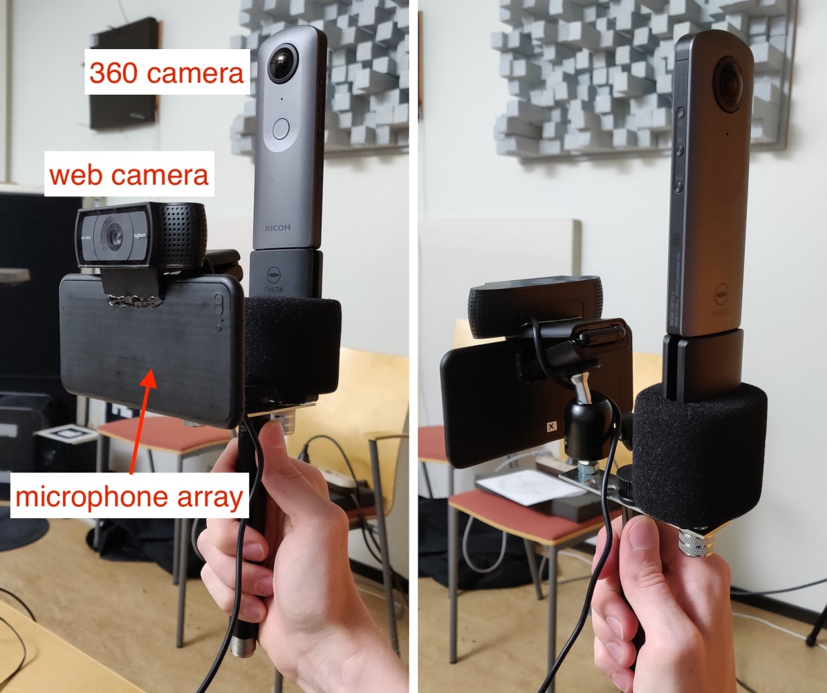
(a) Pictures of the microphone array and other accompanying devices.

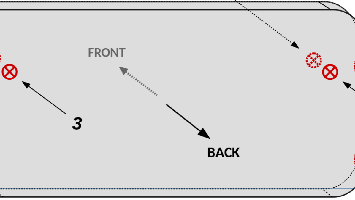
(b) An illustration of the eight microphone placements and the directions ”Front” and ”Back” used to annotate the speaker direction. The x,y,z dimensions of the devices are: 140, 65, and 7 mm.

Figure 1: Recording setup (a), and microphone layout (b).

Database for machine learning

The audio was divided into six different folds. For the first five folds, the data was distributed so that each fold had the same proportion of 1-s blocks captured in an inside and outside environment as the whole data set. Each recording was used as a whole in a single fold, and no recording was split between several folds. The sixth fold includes most data from speech sources simultaneously in front and back. Table II displays the amount of 1-s blocks per each label class. It also includes counts for the cases where speech is present either back or front, and also back and front.

TABLE II: Label appearance statistics for the folds. Note that any combination of labels can be present during a single block.

Fold	Total	Something	Speech Front	No	Speech	Speech	Speech Front
#	blocks	Else	or Back	labels	Front only	Back only	and Back
1	871	376	376	213	187	177	12
2	748	327	310	218	61	243	6
3	768	187	383	305	98	271	14
4	892	292	407	327	173	204	30
5	719	376	201	307	24	176	1
6	1025	0	967	58	291	576	100

III Hierarchical Classification Approach

Given the described labeling scheme, the direct approach is a flat classifier with three multilabel binary output values. The outputs are the presence probabilities for labels ”speech back”, ”speech front” and ”something else”. To solve the task, the model’s input features should contain both spectral and directional information. However, sound event characteristics and direction properties are two very different types of information and therefore challenging to model through a single network. With the hierarchical approach, different types of features or feature representations can be utilized by each task. Therefore, we investigate a hierarchical classifier to first detect the presence of ”speech” and ”something else” classes using magnitude spectral features only. In the second level of the classification, spatial features are extracted and segments already detected to contain speech are further assigned with directional labels of ”speech front” and ”speech back”, where the labels match the sound source direction with respect to the mobile array. The joint system offers a solution to the problem of differing tasks and features. On the other hand, the accuracy of the direction estimation does not only depend on its own performance anymore, since any missed speech samples from the sound event classifier would diminish its performance too. Fig. 2 depicts a high level overview of the proposed system.

III-A Sound Classification (Stage 1)

In the sound classification stage, given a 1-s block of audio, the aim is to recognize if there is speech and/or any other interesting sound events (i.e. ”something else” class) present at any time. The output of this stage is a probability value for both of these labels. Sound classification is done by feeding time-frequency acoustic features extracted from audio to a deep neural network that estimates the class probabilities. Feature extraction and classification are elaborated below.

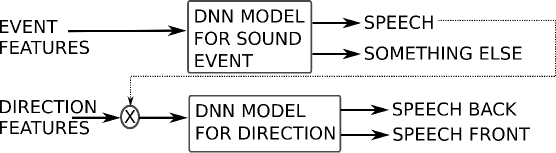
Figure 2: Joint classifier system framework for detection and localization of sound events. First stage detects the type of sound, second stage estimates direction of detected speech.

III-A1 Acoustic Feature Extraction

In a pre-processing step, the multi-channel audio is converted to mono by taking the average over the channels at each sample. The resulting monophonic audio signal is amplitude normalized by dividing with the maximum absolute value.

Log-Mel Spectrogram Estimation

The log-mel spectrogram features were obtained using 20 ms frames and 10 ms overlap in 40 mel frequency bands. The features are standardized to zero mean and unity variance using statistics from the training set.

III-A2 Deep Neural Network Model

The DNN technique utilized in the sound classification is a CRNN. Convolutional layers use small, shifting 2D kernels to extract higher level features that are invariant to local spectral and temporal variations. Recurrent layers are effective in modeling the longer term temporal context for the sound events. Combining convolutional and recurrent layers has been found suitable for various audio classification tasks such as sound event classification [14], automatic speech recognition [30] and music genre classification [31].

The details of the CRNN architecture are as follows. Each 5-by-5 convolutional layer is followed by a rectified linear unit (ReLU) activation, and max-pooling by two in both time and frequency dimensions. The 3D output of the final convolutional layer is converted into 2D by reshaping the frequency and channel dimensions into a single dimension. This output is fed to one or multiple recurrent layers (long-short term memory (LSTM) [32] layers specifically). The LSTM output is fed to a fully connected feed-forward layer with logistic sigmoid activation that applies the same weights over each time step of the input. The resulting output at each time step are the two label probabilities of the i) speech presence using the merged ”Speech Front” and ”Speech Back” labels, and ii) ”Something Else”. Finally, max-pooling over time is applied over the sequence, and the two label probabilities are obtained for the one-second block of audio. The binary label predictions are obtained by using a threshold value of $0.5$ for the output probabilities.

The network is trained to minimize the cross-entropy between the estimate output and the target output. Adam [33] is used as the optimizer. After each epoch, the F1-score for the merged ”speech” labels for the validation set is calculated. If the model does not improve for 25 epochs, the training is terminated. The best model based on the validation set score is used for testing. In total, 197 different hyper-parameter combinations were evaluated with different amounts and configurations of the convolutional layers and the recurrent layers. The best model had 611k learnable parameters.

III-B Localization (Stage 2)

The task of the localization step is to assign the labels of ”Speech front” and ”Speech back” to each 1-s block of audio, detected to contain speech in the first stage. The speaker direction is assumed to be more stable compared to changes in the magnitude spectrum, and therefore longer 85 ms frames with 50 % overlap are utilized. Two types of spatial features are extracted.

III-B1 Time Difference of Arrival (TDoA) Feature

The TDoA, i.e. the sound propagation delay between a microphone pair, brings information about the dominating sound direction during each short processing frame. The case with speakers in front and back is evident by alternating TDoA values.

Since the microphone pair separation in the front-back axis is only 7 mm, the TDoA resolution is limited to three possible values at 48 kHz. Therefore, TDoA is obtained as maximum peak index of Fourier interpolated (factor of five) GCC [34] between microphones.

III-B2 Magnitude Difference Feature

Upon reaching the rigid device, the sound wave is partly reflected and partly diffracted, leading to frequency and angle dependent sound propagation effects. This is observed as a direction specific level difference between the microphones. The magnitude difference between the microphone pairs is used as the second spatial feature to capture this information: $D_{i,j}(b)=\ln(M_{i}(b))-\ln(M_{j}(b))$, where $M_{i}(b)$ is the magnitude of the $b$th mel band of microphone $i$. The total number of mel-bands was $40$.

Features are obtained from two microphone pairs (1,3) and (2,4) located on the front and back surfaces on the left and right side of the device. The pairs are maximally separated in the dimension of interest, refer to Fig. 1(b). Both features are then averaged over the microphone pairs for robustness and to reduce the feature dimension by half.

Deep Neural Network (DNN) Model for Localization

As for sound event detection, the used model was a CRNN, where now two output values are related to probabilities of speech front, and speech back. A similar training process and validation method was used as in Section III-A2. The Adam and Adamax [33] optimizers were experimented with. The training was done using k-fold-cross-validation with all one-second blocks containing speech from the folds listed in Table II. Three of the folds were used for training, two for validation, and one for testing to guarantee sufficient number of directional labels in the validation set. The training was stopped if validation set’s average F1-score over both direction labels started to decrease. Note that the case where both ”Speech front” and ”Speech back” are active is underrepresented, with only 6 % of the samples belonging to this class. As a consequence, the speech samples are labeled as either with ”Speech back” or ”Speech front” labels, and the cases where both labels are active is effectively ignored. To address this data imbalance, a random oversampling strategy [35] was applied to balance training and validation sets during training so that each unique combination of label values (i.e. class) would have the same amount of (partly repeated) training sequences. This reduced slightly the final F1-score in contrast to not using oversampling, but raised the performance of detecting speech in both directions. The best model had 170k parameters.

III-C Baseline

The baseline comparison method is a flat CRNN classifier with three binary labels for each of the classes. The spatial features described in Section III-B are only used, since i) the magnitude spectrum features could not be concatenated to spatial features due to the different frame lengths, and ii) the used spatial features already contain magnitude spectrum difference information. A similar training process as in Section III-A2 is used, but instead of speech-only F1-score, the weighted average F1-score over all three labels is used as the early stopping criteria. The best model had 360k parameters.

IV Evaluation

TABLE III: The confusion matrix of SED (proposed).

white Predicted label [frames] Nothing Speech Else Both True label Nothing 1098 156 162 12 Speech 179 1737 14 126 Else 323 105 465 58 Both 28 139 48 373 white Predicted label [%] Nothing  Speech Else Both Nothing [hsb]0,0.07,17 6.9 [hsb]0,0.01,11 0.9 [hsb]0,0.01,11 1.3 [hsb]0,0.0,10 .8 Speech [hsb]0,0.08,18 .7 [hsb]0,0.08,18 4.5 [hsb]0,0.0,10 .7 [hsb]0,0.06,16 .1 Else [hsb]0,0.03,13 4.0 [hsb]0,0.01,11 1.0 [hsb]0,0.04,14 8.9 [hsb]0,0.06,16 .1 Both [hsb]0,0.04,14 .8 [hsb]0,0.02,12 3.6 [hsb]0,0.08,18 .2 [hsb]0,0.06,16 3.4

TABLE IV: The confusion matrix of SED (baseline).

white Predicted label [frames] Nothing Speech Else Both True label Nothing 1037 194 173 24 Speech 266 1575 38 177 Else 210 152 511 78 Both 40 166 104 278 white Predicted label [%] Nothing  Speech Else Both Nothing [hsb]0,0.07,17 2.6 [hsb]0,0.01,11 3.6 [hsb]0,0.01,11 2.1 [hsb]0,0.01,11 .7 Speech [hsb]0,0.01,11 2.9 [hsb]0,0.07,17 6.6 [hsb]0,0.01,11 .8 [hsb]0,0.08,18 .6 Else [hsb]0,0.02,12 2.1 [hsb]0,0.01,11 6.0 [hsb]0,0.05,15 3.7 [hsb]0,0.08,18 .2 Both [hsb]0,0.06,16 .8 [hsb]0,0.02,12 8.2 [hsb]0,0.01,11 7.7 [hsb]0,0.04,14 7.3

TABLE V: Speech localization confusion matrix (proposed).

white Predicted label [frames] Front Back Both True label Front 676 20 138 Back 23 1558 66 Both 58 28 77 white Predicted label [%] Front Back Both Front [hsb]0,0.08,18 1.1 [hsb]0,0.02,12 .4 [hsb]0,0.01,11 6.5 Back [hsb]0,0.01,11 .4 [hsb]0,0.09,19 4.6 [hsb]0,0.04,14 .0 Both [hsb]0,0.03,13 5.6 [hsb]0,0.01,11 7.2 [hsb]0,0.04,14 7.2

black

TABLE VI: Speaker direction and else class detection performance (A): proposed hierarchical approach, (B): baseline

	Label	Accuracy %	Precision %	Recall %	F1 %
(A)	Speech front	95.2	84.3	89.6	86.9
	Speech back	85.2	79.3	84.4	82.8
	Something else	81.9	75.0	61.3	67.5
	Average (unweighted)	87.4	79.5	78.4	79.1
(B)	Speech front	96.0	92.3	87.1	89.6
	Speech back	82.3	75.8	74.9	75.3
	Something else	80.5	70.2	63.1	66.5
	Average (unweighted)	86.3	79.4	75.0	77.1

Speech Detection Results

The confusion matrix for the two-stage CRNN speech classification model is given in Table III and the baseline results for comparison with speech direction outputs merged into a single class are given in Table IV. The instances where both classes are present are treated as a separate class for the visualization. The sample numbers inside each box are obtained by accumulating the binary output of the test fold values of the six folds using k-fold cross-validation. The percentage values represent the fraction of the predicted labels assigned for each audio block with the corresponding true label.

The hierarchical approach has better classification performance in almost all classes (”Silence”, ”Speech”, ”Both”) except for the ”Else” class in contrast to the baseline.

The ”Something else” performance is quite low in both approaches compared to the class ”Speech”. This can be attributed to i) the labeling ambiguity problem, and ii) to the scarcity of data, which makes it hard to capture the characteristics of all the various types of sound events that are included in this class.

Localization Results

Table V depicts the confusion matrix for the different location classes during frames with annotated speech. The results are obtained by accumulating the binary test folds label predictions over the six folds (i.e. k-fold cross-validation). The direction classifier is described in Section III-B. The speech emitted from the back direction was more accurately recognized than speech from the front. This is expected, since all the samples of a speaker holding the device are labeled with ”Speech back”. Since they were emitted close to the array, they inherently had a better SNR in contrast to the front direction, which contained more distant talkers. The cases where both the directions were active are detected with the least accuracy. This can be attributed to having the least amount (only 6 %) of data from such cases.

Detection and Localization Results

The performance for the joint sound classification and direction detection system is presented in Table VI. In the hierarchical approach, the speaker direction is estimated only when there is speech detected by the sound classifier. For frames without speech detection, the ”Speech front” and ”Speech back” labels are set to zero.

The proposed hierarchical classifier has the highest performance in terms of the F1-score for the labels ”Speech back” and ”Something else”. In contrast, the ”Speech front” is overall better detected with the flat model. This is most likely attributed to the observed difficulty in detecting the presumably more distant and thus weaker speech signals in front of the array. Since the hierarchical system only passes the frames labeled as speech, the performance is deteriorated by the errors accumulating from the two separate classification steps. The ”Speech back” detection capability for the hierarchical model is significantly higher (7.5 % points higher in terms of F1-score) than that of the baseline, rendering the performance of the hierarchical model better in terms of overall performance. This is also evident in the unweighted average performance values, which are all higher for the proposed model in contrast to the baseline.

V Conclusions

This work proposes a two-stage hierarchical sound event detection and localization approach using a mobile microphone array. The first stage of the hierarchical model recognizes the sound event type, and the second stage is invoked for the direction estimation only for the blocks detected to contain speech. This structure allows the utilization of different types of features and network structures for the two stages, and accommodates the use of different hierarchy levels in the annotation of different sound classes.

The proposed method obtained better results in terms of average label score for every metric in contrast to a flat baseline classifier. The use of a mobile phone form factor microphone array and diverse real data pave way for future applications of SELD on practical mobile devices.

In the future, the amount of sound events with direction labels could be increased to study the need for a class specific direction estimation. Similarly, a varying direction resolution for different classes could be investigated.

References

- [1] X. Xiao, S. Zhao, X. Zhong, D. L. Jones, E. S. Chng, and H. Li, “A learning-based approach to direction of arrival estimation in noisy and reverberant environments,” in International Conference on Acoustics, Speech and Signal Processing (ICASSP). IEEE, 2015.
- [2] S. Chakrabarty and E. Habets, “Broadband DOA estimation using convolutional neural networks trained with noise signals,” in Workshop on Applications of Signal Processing to Audio and Acoustics (WASPAA). IEEE, 2017.
- [3] N. Yalta, K. Nakadai, and T. Ogata, “Sound source localization using deep learning models,” Journal of Robotics and Mechatronics, vol. 29, no. 1, pp. 37–48, 2017.
- [4] S. Adavanne, A. Politis, and T. Virtanen, “Direction of arrival estimation for multiple sound sources using convolutional recurrent neural network,” in European Signal Processing Conference (EUSIPCO), 2018.
- [5] J. Vera-Diaz, D. Pizarro, and J. Macias-Guarasa, “Towards end-to-end acoustic localization using deep learning: From audio signals to source position coordinates,” Sensors, vol. 18, no. 10, 2018.
- [6] D. Salvati, C. Drioli, and G. L. Foresti, “Exploiting CNNs for improving acoustic source localization in noisy and reverberant conditions,” IEEE Transactions on Emerging Topics in Computational Intelligence, vol. 2, no. 2, pp. 103–116, 2018.
- [7] F. Vesperini, P. Vecchiotti, E. Principi, S. Squartini, and F. Piazza, “Localizing speakers in multiple rooms by using deep neural networks,” Computer Speech & Language, vol. 49, pp. 83 – 106, 2018.
- [8] P. Pertilä and E. Cakır, “Robust direction estimation with convolutional neural networks based steered response power,” in ICASSP, 2017.
- [9] P. Pertilä and M. Parviainen, “Time Difference of Arrival Estimation of Speech Signals Using Deep Neural Networks With Integrated Time-Frequency Masking,” in International Conference on Acoustics, Speech and Signal Processing (ICASSP). IEEE, 2019.
- [10] Z.-Q. Wang, X. Zhang, and D. Wang, “Robust TDOA estimation based on time-frequency masking and deep neural networks,” in Proc. Interspeech, 2018, pp. 322–326.
- [11] K. J. Piczak, “Environmental sound classification with convolutional neural networks,” in IEEE 25th International Workshop on Machine Learning for Signal Processing (MLSP), 2015, pp. 1–6.
- [12] N. Takahashi, M. Gygli, B. Pfister, and L. Van Gool, “Deep convolutional neural networks and data augmentation for acoustic event recognition,” in Interspeech, 09 2016, pp. 2982–2986.
- [13] J. Salamon and J. P. Bello, “Deep convolutional neural networks and data augmentation for environmental sound classification,” IEEE Signal Processing Letters, vol. 24, no. 3, pp. 279–283, 2017.
- [14] E. Cakır, G. Parascandolo, T. Heittola, H. Huttunen, and T. Virtanen, “Convolutional recurrent neural networks for polyphonic sound event detection,” IEEE/ACM Transactions on Audio, Speech, and Language Processing, vol. 25, no. 6, pp. 1291–1303, 2017.
- [15] T. Hirvonen, “Classification of spatial audio location and content using convolutional neural networks,” in Audio Engineering Society Convention 138. Audio Engineering Society, 2015.
- [16] W. He, P. Motlicek, and J.-M. Odobez, “Joint localization and classification of multiple sound sources using a multi-task neural network,” in Proc. Interspeech 2018, 2018, pp. 312–316.
- [17] S. Adavanne, A. Politis, J. Nikunen, and T. Virtanen, “Sound event localization and detection of overlapping sources using convolutional recurrent neural networks,” IEEE Journal of Selected Topics in Signal Processing, 2018.
- [18] Y. Cao, Q. Kong, T. Iqbal, F. An, W. Wang, and M. D. Plumbley, “Polyphonic sound event detection and localization using a two-stage strategy,” in Proceedings of Detection and Classification of Acoustic Scenes and Events Workshop (DCASE 2019), 2019, pp. 30–34.
- [19] A. Politis, A. Mesaros, S. Adavanne, T. Heittola, and T. Virtanen, “Overview and Evaluation of Sound Event Localization and Detection in DCASE 2019,” IEEE/ACM Transactions on Audio, Speech, and Language Processing, 2020.
- [20] I. Trowitzsch, C. Schymura, D. Kolossa, and K. Obermayer, “Joining sound event detection and localization through spatial segregation,” IEEE/ACM Transactions on Audio, Speech, and Language Processing, vol. 28, pp. 487–502, 2020.
- [21] C. Evers, H. W. Löllmann, H. Mellmann, A. Schmidt, H. Barfuss, P. A. Naylor, and W. Kellermann, “The LOCATA challenge: Acoustic source localization and tracking,” IEEE/ACM Transactions on Audio, Speech, and Language Processing, vol. 28, pp. 1620–1643, 2020.
- [22] M. Harper, “The automatic speech recogition in reverberant environments (ASpIRE) challenge,” in IEEE Workshop on Automatic Speech Recognition and Understanding (ASRU). IEEE, 2015, pp. 547–554.
- [23] J. Barker, S. Watanabe, E. Vincent, and J. Trmal, “The fifth’chime’speech separation and recognition challenge: dataset, task and baselines,” arXiv preprint arXiv:1803.10609, 2018.
- [24] L. Perotin, R. Serizel, E. Vincent, and A. Guérin, “CRNN-based multiple DoA estimation using acoustic intensity features for Ambisonics recordings,” IEEE Journal of Selected Topics in Signal Processing, vol. 13, no. 1, pp. 22–33, 2019.
- [25] T. N. T. Nguyen, W.-S. Gan, R. Ranjan, and D. L. Jones, “Robust Source Counting and DOA Estimation Using Spatial Pseudo-Spectrum and Convolutional Neural Network,” IEEE/ACM Transactions on Audio, Speech, and Language Processing, vol. 28, pp. 2626–2637, 2020.
- [26] E. Hadad, F. Heese, P. Vary, and S. Gannot, “Multichannel audio database in various acoustic environments,” in 14th International Workshop on Acoustic Signal Enhancement (IWAENC), 2014.
- [27] M. Jeub, M. Schafer, and P. Vary, “A binaural room impulse response database for the evaluation of dereverberation algorithms,” in 16th International Conference on Digital Signal Processing. IEEE, 2009.
- [28] R. Stewart and M. Sandler, “Database of omnidirectional and B-format room impulse responses,” in ICASSP, 2010.
- [29] M. Brousmiche, J. Rouat, and S. Dupont, “SECL-UMons Database for Sound Event Classification and Localization,” in ICASSP, 2020.
- [30] D. Amodei, R. Anubhai, E. Battenberg, C. Case, J. Casper, B. Catanzaro, J. Chen, M. Chrzanowski, A. Coates, G. Diamos, et al., “Deep Speech 2: End-to-End Speech Recognition in English and Mandarin,” in 33rd International Conference on Machine Learning, 2016.
- [31] K. Choi, G. Fazekas, M. Sandler, and K. Cho, “Convolutional recurrent neural networks for music classification,” arXiv preprint arXiv:1609.04243, 2016.
- [32] S. Hochreiter and J. Schmidhuber, “Long short-term memory,” Neural computation, vol. 9, no. 8, pp. 1735–1780, 1997.
- [33] D. Kingma and J. Ba, “Adam: A Method for Stochastic Optimization,” in The International Conference on Learning Representations (ICLR), 2015.
- [34] C. Knapp and G. Carter, “The Generalized Correlation Method for Estimation of Time Delay,” IEEE Trans. on Acoust., Speech, and Signal Process., vol. 24, no. 4, pp. 320 – 327, Aug 1976.
- [35] J. Van Hulse, T. M. Khoshgoftaar, and A. Napolitano, “Experimental perspectives on learning from imbalanced data,” in Proc. ICML’07, 2007, pp. 935–942.