Multi-objective Evolutionary Approach for Efficient Kernel Size and Shape for CNN
Abstract
While state-of-the-art development in Convolutional Neural Networks (CNNs) topology, such as VGGNet and ResNet, have become increasingly accurate, these networks are computationally expensive involving billions of arithmetic operations and parameters. In order to improve the classification accuracy, state-of-the-art CNNs usually involve large and complex convolutional layers. However, for certain applications, e.g. Internet of Things (IoT), where such CNNs are to be implemented on resource-constrained platforms, the CNN architectures have to be small and efficient. To deal with this problem, reducing the resource consumption in convolutional layers has become one of the most significant solutions. In this work, a multi-objective optimisation approach is proposed to trade-off between the amount of computation and network accuracy by using Multi-Objective Evolutionary Algorithms (MOEAs). The number of convolution kernels and the size of these kernels are proportional to computational resource consumption of CNNs. Therefore, this paper considers optimising the computational resource consumption by reducing the size and number of kernels in convolutional layers. Additionally, the use of unconventional kernel shapes has been investigated and results show these clearly outperform the commonly used square convolution kernels. The main contributions of this paper are therefore a methodology to significantly reduce computational cost of CNNs, based on unconventional kernel shapes, and provide different trade-offs for specific use cases. The experimental results further demonstrate that the proposed method achieves large improvements in resource consumption with no significant reduction in network performance. Compared with the benchmark CNN, the best trade-off architecture shows a reduction in multiplications of up to 6X and with slight increase in classification accuracy on CIFAR-10 dataset.
Index Terms:
Convolutional Neural Networks, Evolutionary Computation, Deep Learning, Multi-Objective Evolutionary OptimisationI Introduction
Deep Neural Networks (DNNs) are biologically-inspired computing systems which consist of internal connections between artificial neurons. In recent years, DNNs have drawn increasing attention in various application domains, such as image processing, speech recognition and many other challenging Artificial Intelligence (AI) tasks (Guo et al., 2016a, ). In particular, Convolutional Neural Networks (CNNs) have successfully gained outstanding performance in image classification and video recognition (LeCun et al.,, 1998; Zhao et al.,, 2019; Ren et al.,, 2017). In general, the common CNN architecture usually consists of convolutional layers and pooling layers in between its input layer and fully-connected output layer. The convolutional layers and pooling layers in CNNs are sparsely connected. Compared with the conventional fully-connected layer in a feed-forward neural network, neurons in a convolutional layer are only connected with several neurons in the previous layer. Specifically, any neuron in the feature map of a convolutional layer is a linear combination of neurons in the receptive field which is defined by a convolution kernel in the previous layer (Goodfellow et al.,, 2016; Yu and Koltun,, 2015). The state-of-the-art achievements of designing CNN architectures have demonstrated significant improvements on network classification accuracy on various benchmark datasets, such as GoogleNet (Szegedy et al.,, 2015) and AlexNet (Krizhevsky et al.,, 2012). In order to get the best accuracy on specific tasks, the computational complexity of the network grows exponentially and this brings new challenges of executing it on resource-constrained platforms. Based on the analysis by Canziani et al., (2016), several low-cost network architectures can still achieve reasonable accuracy on state-of-the-art benchmark datasets. The motivation to find CNN architectures that can achieve high accuracy and keep computational resource usage at a minimum is therefore high.
Multi-objective evolutionary algorithms (MOEAs) are today one of the most commonly used methodologies in solving hard optimisation problems where two or more (multiple) conflicting objectives must be satisfied simultaneously (Coello,, 2001). MOEAs aim to generate a set of possible solutions (so-called population) in a single run of the algorithm. In recent years, there have been several research studies focusing on optimising neural network typologies and their connection weights. These approaches have demonstrated that using evolutionary algorithms to evaluate neural network topology can achieve competitive performance on state-of-the-art benchmark datasets (Xie and Yuille,, 2017; Suganuma et al.,, 2017; Moriarty and Miikkulainen,, 1998).
In this article, we investigate optimisation of feed-forward CNN architectures for use in resource-constrained scenarios using MOEAs. In order to achieve a high classification accuracy, state-of-the-art CNN architectures are extremely complex. For example, AlexNet (Krizhevsky et al.,, 2012) requires billions of multiply-accumulation (MAC) operations to process a single image. In general, convolutional layers are the most computationally expensive ones, where the resource consumption in each layer is proportional to the number and sizes of the convolution kernels. For instance, a convolution kernel requires more than twice the number of MAC processes than a kernel. Therefore, to reduce the resource consumption in convolutional layers, we aim to reduce the number of MAC processes in these layers by using unconventional kernel shapes as well as reducing the number of kernels in each convolutional layer with minimum loss of network accuracy. The conventional approach to designing the convolutional layer in CNNs is using a set of square convolution kernels which extract the image features. However, the conventional kernels are computationally costly where a large number of multiplications is needed to calculate each feature map. Sironi et al., (2014)explore the idea of separable convolutions, where a set of smaller 1D convolution kernels is designed to replace the conventional 2D ones. For example, a specific matrix can be replaced by the product of a matrix times a matrix, instead of calculating one convolution with 9 MAC processes, the reformulation calculates two convolutions with 3 MAC processes each, totally 6 MAC processes, to achieve the same performance for specific tasks. The caveat is that this separation only works within certain constraints, i.e. only a subset of matrices with specific properties can be replaced. Our proposed design contains a number of differently shaped kernels, including 1-D kernels, 2-D rectangle kernels and 2-D square kernels. Each of these kernels can have a different shape and size which require different numbers of MAC processes to extract the features from the input images. In order to minimise the resource consumption and retain the network accuracy while processing the CNNs on the target hardware platform, we use the fast Non-dominated Sorting Genetic Algorithm (NSGA-II) (Deb et al.,, 2002) to explore the design space for the feed-forward CNN architecture and produce the best trade-off between network complexity and classification accuracy. Our proposed method is focusing on optimising the network width using combinations of various unconventional shapes and sizes of kernels, while keeping the depth constant. Moreover, to further reduce resource consumption of convolutional layers, the optimisation approach described in this paper also aims to minimise the number of kernels used in the convolutional layers. The proposed method is tested on widely-used benchmarks, the MNIST (LeCun et al.,, 2010), Fashion-MNIST (Xiao et al.,, 2017) and CIFAR-10 (Krizhevsky and Hinton,, 2010) datasets, and compared with conventional CNNs. The proposed method produces a range of network architectures, with some solutions achieving a factor of 5.93X saving in computational resource consumption with a 0.09% improvement on classification accuracy on CIFAR-10 benchmark dataset. This paper proposed a methodology that can significantly reduce computational cost of CNNs, based on unconventional kernel shapes, and provide different trade-offs for specific use cases.
The paper is organised as follows: Section II gives an overview of the current approaches of optimising feed-forward neural network architecture, as well as optimising learning algorithms and hyperparameters. Section III describes the design methodology that implements NSGA-II to explore the design space of CNN architecture and explains its features. Section IV shows several test experiments with varying benchmark datasets and provides a proof-of-concept of the performance of the proposed method. Finally, Section V concludes the paper and discusses further work.
II Related Works
This section introduces a review of the current approaches of automatic optimisation techniques that are used to find good solutions by network topology optimisation, such as connection weights, network structure.
II-A Optimisation of Network Architecture
Evolutionary Algorithms (EAs) are widely used in optimisation problems with complex fitness landscapes. The main idea of optimising artificial neural networks using EAs is to evolve the synaptic weights and connections of the network (Moriarty and Miikkulainen,, 1998). NEAT (Stanley and Miikkulainen,, 2002) is a method that uses genetic algorithms (GAs) to change both connection weights and network structure. Their proposed method encodes each neuron and synaptic weight in the genotype. For each iteration, the GA can either add additional neurons to the network or adjust the input/output connections of a neuron. This method allows the GA to find out the best network topology for the target task. A hypercube-based NeuroEvolution of Augmenting Typologies (HyperNEAT) method has shown advantages when optimising weights for CNNs (Stanley et al.,, 2009; Verbancsics and Harguess,, 2015). However, due to the lager search space of CNN topologies, this method requires huge amounts of computational resources. Therefore, this method is difficult to scale up to state-of-the-art deep neural network architectures, because of their size. Morse and Stanley, (2016) compared evolutionary algorithms with the stochastic gradient descent (SGD) method for weight optimisation of ANNs. Their results demonstrate that using an evolutionary algorithm to optimise weights achieves competitive results, compared with the traditional SGD method.
From these previous approaches, it is reasonable to assume that GAs are a suitable method for optimising network topology. However, for network weight optimisation, GAs show almost the same performance as SGD through back-propagation. Therefore, in order to search for efficient neural network architectures and updating network weights at the same time, a combination of GAs and SGD methods have been investigated in recent years. Real et al., (2017) apply GAs to CNN design, where the model is trained by SGD through back-propagation and the architecture is optimised by simple GA. They initialise the starting point as a small model which only consists of a single pooling layer. With each evolutionary step, the model is grown by adding more convolution layers. Their approach is only focusing on network accuracy, therefore, the result shows that as the network accuracy is increased, the computational effort required is increased dramatically. CoDeepNEAT (Miikkulainen et al.,, 2019) is a further extension of NEAT (Stanley and Miikkulainen,, 2002) where the population is separated into two sub-sets: module and blueprint. The module chromosome is a graph that represents a small ANN and the blueprint chromosome is a graph where each mode contains a pointer to a particular module species. During the evolution, the two sub-sets are combined together to build a larger network, where each mode in the blueprint is replaced with a module chosen randomly from the species to which that mode points. Their results show that the network designed by CoDeepNEAT can achieve competitive accuracy in image classification problems with faster training speed. Kim et al., (2017) use a multi-objective evolutionary algorithm (MOEA) to trade-off between classification accuracy and run-time. They adopt NSGA-II to explore the Pareto front of the design space. The network architecture is decoded into two categories: number of outputs in each layer and the total number of convolution layers. Their experimental results show that multi-objective optimisation can further reduce the run-time and achieve better accuracy compared with human-expert design. Xie and Yuille, (2017) present a GA solution for searching large-scale CNNs. In their work, the GA is applied to designing the network structure, where the connectivity of each layer is encoded by a binary string representation. This method can be easily modified for different network architectures and includes different types of layers and connectivity.
Apart from using GAs to optimise the CNN architecture by pre-processing the initial populations, such as pre-defining the layer functionalities and connectivity, there are also some GA-based fully automatic architecture design methods addressed in recent years, e.g. Sun et al., (2018). Their design methodology contains a building block that directly using a skip layer to replace the convolutional layer. The skip layer contains two convolutional layers and one skip connection, where the skip connection connects the input of the first convolutional layer to the output of the second convolutional layer. Then, a GA is applied to searching suitable connections of skip layers and pooling layers. Finally, fully-connected layers are added to the tail of the CNN. Similarly, Suganuma et al., (2017) proposes using Cartesian Genetic Programming (CGP) (Miller and Harding,, 2008) to represent deep neural network architectures and to use highly functional modules as the node functions to reduce the search space. There are six different node functions in their design, including convolutional blocks, residual blocks, max and average pooling, etc. The CGP encodes CNNs as directed acyclic graphs with a two-dimensional grid of nodes. Their results demonstrate that the architectures built by CGP outperform most of the hand-designed modules and provide a good trade-off between classification accuracy and the number of parameters.
II-B Optimisation in Training
A large number of hyperparameters need to be configured when designing and training a neural network. These hyperparameters, such as the learning rate, regularisation coefficients and number of training iterations, have significant impact on the convergence efficiency of the training process when considering computational cost. Grid search (Larochelle et al.,, 2007) and random search (Bergstra and Bengio,, 2012) have been previously used to find local optima for the values of hyperparameters in the multi-dimensional search space. Bergstra and Bengio, (2012) have demonstrated an optimisation method for hyperparameters based on random search. In their approach, multiple hyperparameters have been considered for optimising a 3-layer network. They have compared the performance between grid search (Larochelle et al.,, 2007) and random search for optimising neural networks. The results show that optimisation through random search can converge to local optima more efficiently than grid search when given the same computing budget, especially for high-dimensional spaces.
A recent state-of-the-art optimisation technique for hyperparameters in neural networks is Bayesian optimisation. Different from grid search and random search, where each evaluation is processed by purely random sampling of points in the search space, Bayesian optimisation with Gaussian Process (Rasmussen,, 2003) uses prior solutions of the objective function to determine which objective in the search space needs to be evaluated next. In this method it is assumed that in each dimension of the search space, the distribution of the objective function can be modelled as a Gaussian distribution centred on the mean value of the objective function separately for each dimension. Snoek et al., (2012) proposed an optimiser based on Bayesian optimisation which considers nine hyperparameters in a CNN, including learning rate, number of epochs etc. Their approach shows that Bayesian optimisation of hyperparameters in CNNs can outperform human-expert designs in terms of classification accuracy. Additionally, an optimisation method for artificial neural networks with a Gaussian Process search algorithm demonstrates significant reduction in both computing time and error rate, compared with random search and grid search (Dernoncourt and Lee,, 2016). Swersky et al., (2013) proposed a multi-task Bayesian optimisation method where the knowledge is transferred between a finite number of correlated tasks. Their method separates a large dataset into several smaller subsets, then uses these subsets to find the best settings of hyperparameters for the full dataset by evaluating the configuration of subsets.
II-C Unconventional Convolutions
Traditional CNN designs use square kernels to detect the image features. This design method brings significant challenges for computational systems, because the number of arithmetic operations increases exponentially as the network size increases. In order to reduce computational resource usage and speed up large CNNs, recent research using unconventional kernel shapes has focused on approximating existing square-kernel convolutional layers for network compression and acceleration. Recent approaches (Sironi et al.,, 2014; Jaderberg et al.,, 2014; Denton et al.,, 2014) have demonstrated that some of the 2-D square convolution kernels can be factorised into two 1-D kernels. For example, if a convolutional layer contains a set of 2-D kernels, where represents the kernel height and width, it can be factorised as a sequence of two layers with and kernels, which uses less computations. Therefore, the 1-D convolution approximation can significantly accelerate the classification speed as well as reducing the number of network parameters. Similarly, Jin et al., (2014) introduce this into the training phase by factorising a conventional 3-D convolution kernel into three consecutive 1-D kernels. Their results show that by factorising the 3-D convolution layers, the network can be accelerated by approximately a factor of two while sustaining similar or better classification accuracy than using conventional 3-D convolution kernels.
Another approach to design the convolutional layer is to use multiple sizes of kernels in one layer. GoogleNet (Szegedy et al.,, 2015) is one of the most accurate CNNs on state-of-the-art benchmark datasets. In order to increase the network accuracy, their work introduces an inception module to increase the network depth and width. Firstly, the inception module contains multiple differently-sized convolution kernels, as well as max pooling operations. Different types of kernels are computing in parallel and extract features at multiple scales. After that, feature maps from different kernels are concatenated to form the input of the next module. In order to reduce the computational effort, a kernel convolution is inserted into the inception module for dimension reduction. Hence, the network can grow deeper and wider with reasonable increase in computational resource usage. Szegedy et al., (2016) modify the inception module, where the convolution kernels are replaced by a sequence of and kernels, so that the overall computing resources are reduced when compared with the original design. Ding et al., (2019) propose Asymmetric Convolution Blocks (ACBs) to replace the conventional convolution kernels. Typically, ACBs replace the conventional convolutional layer with three parallel layers, where these layers contain , and kernels respectively. Finally, the outputs from each layer are summed up to enrich the feature space.
II-D Other Methods for Reducing Computational Complexity
Vector Quantization (VQ) is a method for compressing densely connected layers to make CNNs smaller. VQ is a method that quantises groups of numbers together (Gersho and Gray,, 2012). Compared with scalar quantisation, VQ can significantly reduce computational and memory resource usage. This is because scale quantisation needs to address every input data one by one (Sullivan,, 1996), VQ can process a set of numbers concurrently. The disadvantage is that in order to reduce the computational and memory resource usage, VQ always has some loss of accuracy. Denil et al., (2013) introduce that there are redundancies in neural network parameters. Then, they apply VQ to reduce the number of dynamic parameters in deep models by representing the weight matrix as a low-rank product of two smaller matrices. Su et al., (2018) follows the research on reducing network redundancy for implementing artificial neural networks on FPGAs. Their work suggests that the network redundancy can be reduced at the data level as well as the model level. The hardware system, after reducing network redundancies, shows that both logic resources and on-chip memory usage can be reduced. Since deep CNN models involve millions of parameters, Gong et al., (2014) have investigated information theoretical vector quantization methods for compressing the parameters of CNNs. Their results show that the VQ method has a significant improvement over existing matrix factorisation methods. After 16 to 24 times compression of state-of-the-art CNNs, the classification accuracy only has a 1% loss.
There is an alternative approach to reducing both the number of operations and parameters, i.e. pruning. The pruning method aims to reduce the number of parameters and operations in CNNs by permanently dropping less important inner-connections (Hanson and Pratt,, 1989). The pruning method allows large predecessor networks to inherit knowledge from a smaller network and maintain comparable accuracy. Han et al., (2015) introduce a method that prunes the network by thresholding the magnitude of weights. If the absolute magnitude of any weight parameter is less than a scalar threshold value, the weight will be pruned. The weight magnitude-based method shows that with network pruning, it can significantly reduce the memory requirement for storage of the neural network as well as the number of neuron connections, without affecting accuracy. Guo et al., 2016b continued this research applied to magnitude-based pruning methods. The method proposed allows restoration of the pruned weights by iteration. allows the network to be pruned at each iteration and can significantly reduce the network complexity for large CNN models without any loss in accuracy.
In summary, although, the overall computational resources are reduced by applying the 1-D convolution kernels, those 1-D convolution kernels also lower the networks’ classification accuracy. There are still a gap needed to be filled. Is there a combination of non-square convolution kernels for CNNs that can reduce the computational costs and remain the same or even higher the classification accuracy at the same time? Furthermore, previous researches only focus on developing 1-D convolution kernels, weather other shapes of unconventional convolution kernels can gain CNN’s performance also needs to be investigated. The rest of this paper proposes a new method to address the problem that provide different trade-offs between the CNNs’ computational costs and classification accuracy based on finding out the combination of unconventional convolution kernels.
III Methodology
The main idea in this work for optimisation of the CNN architecture is to consider how the classification accuracy can be improved (or kept the same) while reducing the computational resources required. Literature of previous investigations suggests that using different shapes of convolution kernels can improve the network performance by detecting multiple-scale features from input images (Ding et al.,, 2019). In this section, an analysis into how the size and shape of the convolution kernels are processed regarding to their computational resource consumption is conducted. Then, a set of different shapes of convolution kernels is designed to be used in convolutional layers. The MOEA used is NSGA-II (Deb et al.,, 2002) to automatically discover efficient network architecture by finding the trade-off between the computational complexity and module classification accuracy on the three benchmark datasets.
III-A Computational Resource Consumption
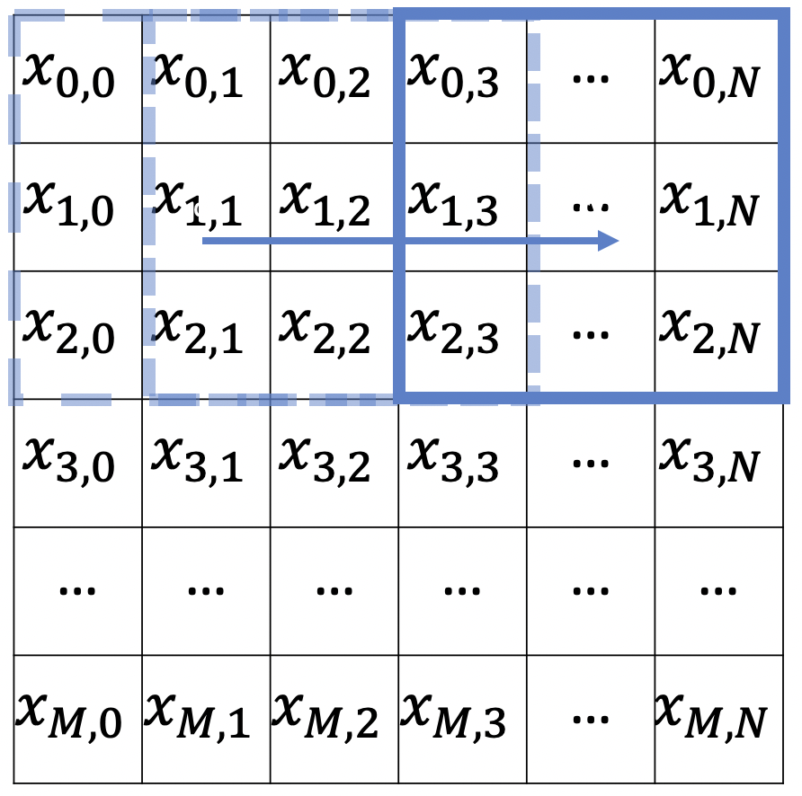
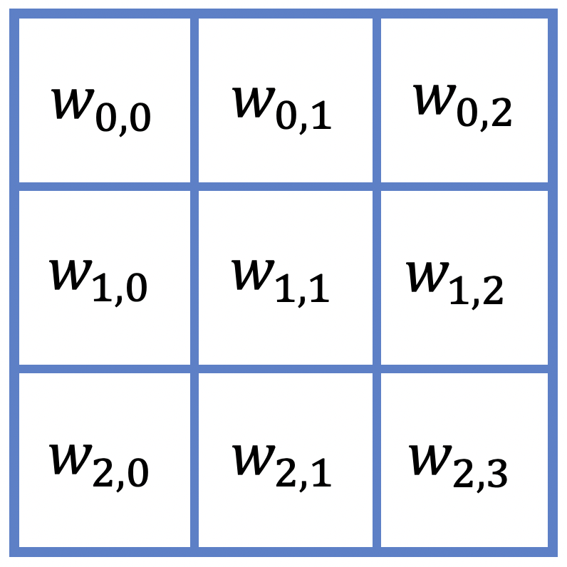
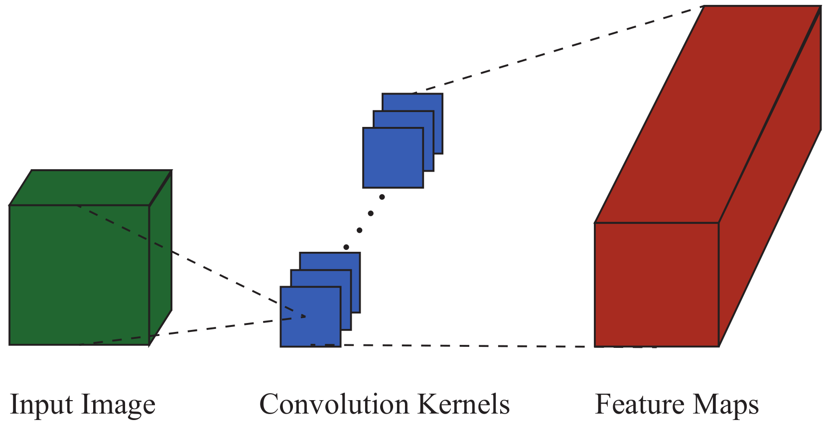
For state-of-the-art CNN architectures, the computationally most expensive parts are the convolutional layers (Canziani et al.,, 2016). In a feed-forward CNN, the convolutional layers are used to extract features from input images. The conventional 2-D convolution process is illustrated in Fig. 10. Mathematically, the formulae for calculating a single feature map by convolution operation can be described as (1),
| (1) |
where is an output feature map of the convolutional layer in the -th channel, I is the input image of the convolutional layer with channels, is the set of 2-D convolution kernels in current layer and represents the convolution operation. It can be seen from the equation, the calculation consists of repeatedly accumulating multiple kernels to form a number of feature maps, which represent the different characteristics of the input image.
Processing a CNN in hardware requires multiply-accumulation (MAC) operations to obtain the output feature maps. In order to improve the classification accuracy of CNNs, state-of-the-art CNN architectures have become increasingly complex, therefore, it is necessary for CNN designs to consider their computational resource consumption.
For a convolutional layer, the number of MAC processes is contingent on the size of the convolution kernels, number of kernels and the size of the output feature maps. It can be calculated using following equation:
| (2) |
where and indicate the height and width of the output feature maps and represents the number of output feature maps, i.e. output channels. Similarly, , and indicate the height, width and the number of the convolution kernels in the corresponding layer. In the conventional design methodology of CNNs, feature maps and convolution kernels are always square, which means the height and width of the convolution kernels and feature map are the same.
In a CNN, the fully-connected layer takes the output of the previous convolution processes and predicts the best classification that is labelled to describe the image. Equivalent to (2), the number of operations in the fully-connected layer of a specific CNN can be calculated as:
| (3) |
where the , and indicate output feature maps from the last convolutional or pooling layer and is the number of neurons in the fully-connected layer.
As can be seen from (2) and (3), the convolutional layer requires more MAC operations than the fully-connected layer. Therefore, reducing the number of MAC operations can significantly reduce the computational resource consumption overall. This is important to allow state-of-the-art CNNs to be processed on resource-constrained platforms, such as FPGAs and embedded devices. Apart from the convolutional layers and fully-connected layers, the CNN architecture also involves other layers, including average pooling, max pooling or batch normalisation. For instance, average pooling is used to calculate the average number of pixels in the kernel and max pooling is proposed to find the maximum number of input pixels, which are smaller than operations for convolutional layers in real cases.
III-B Mixed Unconventional Kernels
In this work, in order to minimise the hardware costs while maintaining the CNN classification accuracy, the MAC operations in the convolutional layers are minimised by reducing the kernel sizes, i.e. the product of and in (2). For example, a 2-D convolution kernel can be replaced by a kernel followed by kernel, which reduces the number of operations from 9 to 6. However, previous research suggests that the replacement is not equivalent as it does not work as well on some of the lower level layers (Szegedy et al.,, 2016), and not all possible kernels are captured by the decomposition. Hence, such a substitution requires the network to have extra kernels or layers to compensate, which may potentially increase again the computational complexity. Therefore, the first question to investigate here is what kinds of kernels can be replaced by smaller ones in a convolutional layer. In addition, without adding an additional convolution kernels, it is investigated whether the conventional 2-D square kernels can be directly replaced by more generic sizes of shape kernels. Finally, the best combination of different shapes and sizes of kernels for each convolutional layer is considered.
Utilising different kernel sizes allows the network to extract features at multiple scales (Szegedy et al.,, 2015). It is becoming more popular for state-of-the-art CNN architectures to use small kernels, such as and . Therefore, the largest kernel selected for the network architecture proposed here has a size of . In order to find the best combination of kernel shapes in a convolutional layer, conventional square kernels and 1-D kernels are used as well as other sizes of kernels, such as and . In total there are 9 different sizes of kernels considered here, the largest being and the smallest one , as shown in Fig. 11.

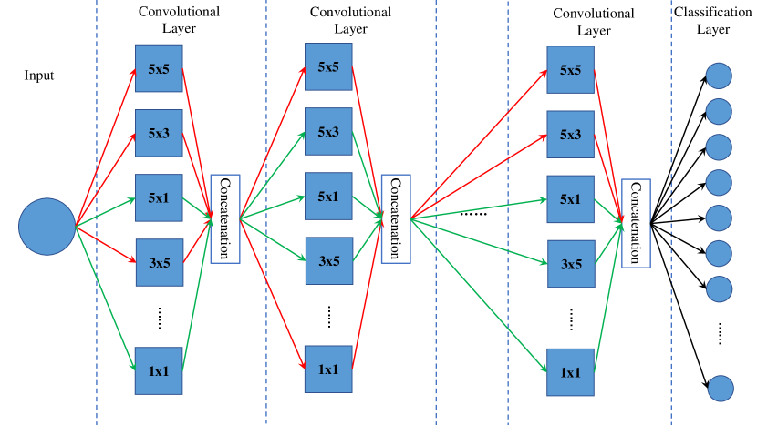
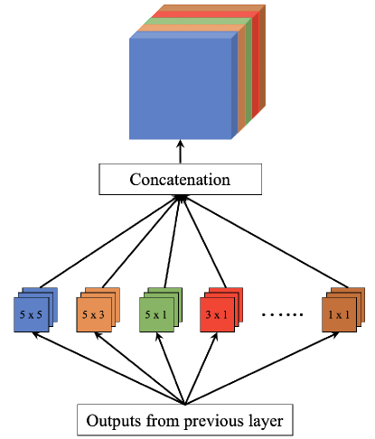
Previous approaches have shown that it is possible to use a series of kernels with differing sizes to better handle multiple-scale objects in a convolutional layer (Szegedy et al.,, 2015). Rather than using conventional square kernels, this work puts the set of 1-D stripe kernels into a single convolutional layer. This is so that the network can operate in parallel on different sizes with the most accurate detailing, , to the biggest kernels, . Then, all feature maps generated from the different kernels are concatenated together into a single output tensor in order to form the input of the next stage. Padding strategy are applied to make sure that the output feature maps from each set of unconventional kernels will have the same resolution as others. Then, the concatenation are used to combine the output feature maps from each set of unconventional kernels into one output tensor. The overall architecture of the proposed design can be viewed as Fig. 12.
III-C Multi-Objective Evolutionary Optimisation
Following the convolutional layer design methodology from the previous section, it is difficult to define the optimal kernel sizes required to replace the conventional square kernels in a given CNN architecture. The new methods described here propose to use the non-dominated sorting genetic algorithm (NSGA-II) to explore the kernel size design space of the CNN architecture. NSGA-II is one of the most popular multi-objective optimisation algorithms which uses a fast non-dominated sorting approach and diversity preservation (Deb et al.,, 2002). The approach of optimising for Pareto optimality makes it possible to trade-off between network accuracy and hardware resource consumption. An overview of optimising a given CNN architecture is shown in Fig. 13.
In the optimisation loop, each of the possible unconventional kernel shapes is identified with its kernel ID that represents a specific kernel. As shown in Fig. 13, the optimisation loop takes a given conventional CNN architecture as its input.
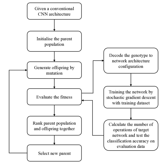
The kernels from all layers of the input CNN are encoded in the genotype. As we are focusing on optimising the convolutional layers, other hyperparameters of the network are kept the same as in the input CNN, e.g. other types of layers, stride, activation function and number of layers. The initial parent population of NSGA-II is generated by randomly replacing the original square kernels with randomly selected unconventional kernel sizes for all convolutional layers in the network. After the initial parent population is created, the first offspring population is generated by mutation operation, which changes the shape of randomly selected kernels based on a given probability. In this case, the genetic representation only consists of a single chromosome, a vector encoding the kernel shapes. Crossover operation is not used in this case.
Then, the fitness of each individual in the population is evaluated by calculating the number of operations in the convolutional layers and testing the classification accuracy of the trained model on a validation set. The architecture generated by NSGA-II is trained using stochastic gradient descent (SGD), using a model training dataset. In this design, one of the fitness measures of NSGA-II is the classification accuracy which is defined as the Top-1 accuracy of trained model on the test dataset. Another fitness is the summation of MAC operations required to compute all of the convolutional layers in the network, which is calculated by (2).
Finally, NSGA-II ranks the fitness of each individual by using a non-dominated sorting approach and a diversity preservation strategy to ensure selection with elitism and a uniform spread of solutions. In non-dominated sorting, each solution has two entities: the first is domination count, the number of solutions that dominate ; the second is the number of solutions that dominates. All solutions will be sorted according to each solution’s domination count into multiple ranking levels. Diversity preservation is achieved by adopting a crowding distance comparison. So that, when there are two solutions with the same domination level, the one that resides in less densely populated points of the solution space is selected (Coello,, 2006). Following this, half of the individuals which have higher rank will be selected as the parent population for the next generation.
IV Experimental Setup and Results
Each individual’s fitness needs to be evaluated separately by training and testing the resulting network. State-of-the-art CNN architectures may require extremely large computational budgets for processing the networks. The aim in this paper is to show the improvement of the proposed method compared with conventional convolutional layers in terms of trade-off between computation costs and classification accuracy. Therefore, a small CNN, the Lenet-5 architecture, is used here as the benchmark network to illustrate the improvement achieved by our proposed method. To evaluate the capability and the full potential for scalability of the proposed method, it is also tested on deeper CNN architectures.
IV-A Experimental Settings
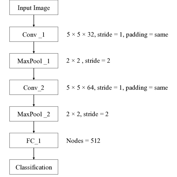
The benchmark CNN architecture is built based on the Lenet-5 architecture (LeCun et al.,, 1998). The original Lenet-5 consists of two convolutional layers and two max-pooling layers, a fully-connected layer and a classification layer. In order to improve the classification accuracy of the network, we increase the number of kernels in each of the convolutional layer and nodes in the fully-connected layers. The overall architecture is shown in Fig. 14, which is used as the benchmark topology to test the proposed method.
The optimisation method is applied to three different datasets, MNIST, Fashion-MNIST and CIFAR-10. MNIST and Fashion-MNIST consist of a training set of 60,000 images and a test set of 10,000 images. Each image in the two MNIST sets is a grayscale image, associated with a label from 10 different classes. CIFAR-10 is split into a training set of 50,000 images and a test of 10,000 images. Each image in the CIFAR set is a pixel RGB image, associated with a label from 10 different classes. The network is trained on the training sets and evaluated in the test set, which is one of the fitness measures of the proposed method. The number of operations is calculated by the total number of multiplications in two convolutional layers, the second objective measure used here. All of the networks are trained by SGD method and use the Adam optimiser (Kingma and Ba,, 2014) with a learning rate of 1e-3. The softmax cross-entropy loss is used as the loss function. Each model is trained for 30 epochs.
In order to explore the Pareto front of the CNN architecture, the optimisation loop is set to run 100 generations for a population size of 25 individuals. There is only one type of chromosome. Hence, only mutation is used as the genetic operator, the mutation rate is 0.1.
IV-B Two-Objective Optimisation
The proposed method is evaluated on CIFAR-10 dataset using two optimisation objectives, number of multiplications in convolutional layers and network classification accuracy. In this experiment, the training dataset is created by randomly selecting 40,000 images from the training set, and the remaining 10,000 images are used for fitness evaluation. Finally, architectures found are trained on the training set for 100 epochs and classification accuracy is tested on test set. To prevent overfitting, a weight decay of 0.0001 and data augmentation have been used for training the networks. The data augmentation used is based on He et al., (2016), that is padding 4 pixels on each side and randomly crop a patch from the padded image or its horizontally flipped version. In order to handle the colour image inputs, the input layer of the benchmark network is modified as 3 channel input.
After configuring the benchmark network to accept colour images, the total number of multiplications required for the convolutional layers further increases to 15,564,800, and the classification error is 17.63% on CIFAR-10. The optimisation loop has a population of 25 individuals and was run for a 100 generations. Three different architectures from the set of solutions are chosen as reference points. The first reference point, Ref 1, has the highest accuracy. The second reference point is one which involves significantly less computational resource while still featuring high accuracy. The third reference point is the trade-off solution closest to the origin between number of multiplications and classification accuracy. The optimisation results and details of kernels usage of three reference architectures can be viewed in Appendix A.
These three architectures are then re-trained on the whole training set, i.e. 50,000 images for training, and the classification accuracy is evaluated on the test set which contains 10,000 examples. Each architecture is re-trained for 100 epochs with weight decay and data augmentation. All of them are trained by using Adam optimiser (Kingma and Ba,, 2014) with initial learning rate of 0.001 and the learning rate is reduced by factor of 10 at 30th epoch. After re-training and testing, the results are shown on Table I. The comparison between the benchmark network and reference point is shown in Table I.
Then, the proposed method is tested on MNIST and Fashion-MNIST datasets. With the same training settings, the benchmark network has a classification accuracy of 98.92% on MNIST and 98.92% on Fashion-MNIST. Both benchmark networks require a total of 10,662,400 multiplications in their convolutional layers. There are three reference solutions that have been selected from each set of solutions using the same approach as before: the first reference solution features the highest accuracy, the second reference solution uses less resources while featuring high accuracy, and the third reference solution has the closest-to-origin trade-off between number of multiplications and classification accuracy. The full optimisation results and details of kernels usage of three reference architectures in each dataset can be viewed in Appendix A.
| Dataset | Model | Top-1 Acc. | Acc. improve | Reduction in Mults. |
|---|---|---|---|---|
| MNIST | Benchmark | 98.92% | - | - |
| Ref 1 | 99.56% | 0.64% | 2.15x | |
| Ref 2 | 99.54% | 0.62% | 3.13x | |
| Ref 3 | 99.49% | 0.57% | 7.02x | |
| Fashion-MNIST | Benchmark | 92.12% | - | - |
| Ref 1 | 93.14% | 1.02% | 2.95x | |
| Ref 2 | 93.07% | 0.95% | 4.24x | |
| Ref 3 | 92.79% | 0.67% | 9.15x | |
| CIFAR-10 | Benchmark | 82.37% | - | - |
| Ref 1 | 83.75% | 1.38% | 2.71x | |
| Ref 2 | 82.54% | 0.17% | 4.06x | |
| Ref 3 | 80.84% | -1.53% | 7.14x |
IV-C Three-Objective Optimisation
Based on the experimental results reported in the previous section using two objectives, an additional step is considered with the aim to further reduce the number of multiplications in convolutional layers by allowing the proposed method to remove kernels if possible. A third objective has been added to the optimisation loop accordingly, which is the number of kernels. As described in Section III, the number of operations of convolutions will also be reduced by using fewer kernels. Therefore, the number of kernels is a secondary measure that puts optimisation pressure on reducing the resource consumption of the networks. The proposed method is now aiming to find the trade-off between three objectives, i.e. number of multiplications used in convolutional layers, model classification accuracy and number of kernels used in each layer. The benchmark CNN is the same LeNet-5 architecture with the original set of kernels as used in the previous experiments.
In this case, two different architectures are chosen which are found by the 3-objective method from each dataset as reference points and compared with the benchmark network that has been used in previous comparisons. The results for optimising two layer network with three objective optimisation on MNIST, Fashion-MNIST and CIFAR-10 are shown in Table II.
| Dataset | Model | Top-1 Acc. | Acc. improve | Reduction in Mults. |
|---|---|---|---|---|
| MNIST | Benchmark | 98.92% | - | - |
| Ref 1 | 99.52% | 0.60% | 2.84x | |
| Ref 2 | 99.48% | 0.56% | 7.04x | |
| Ref 3 | 99.38% | 0.46% | 18.38x | |
| Fashion-MNIST | Benchmark | 92.12% | - | - |
| Ref 1 | 92.96% | 0.84% | 3.74x | |
| Ref 2 | 92.75% | 0.63% | 8.12x | |
| Ref 3 | 92.67% | 0.55% | 11.03x | |
| CIFAR-10 | Benchmark | 82.37% | - | - |
| Ref 1 | 83.47% | 1.10% | 2.85x | |
| Ref 2 | 82.46% | 0.09% | 5.93x | |
| Ref 3 | 80.73% | -1.64% | 8.03x |
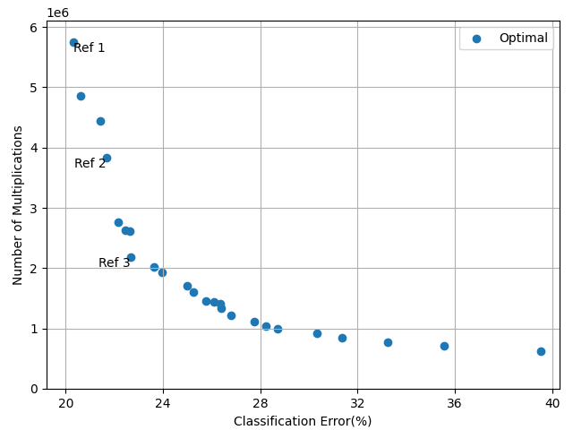
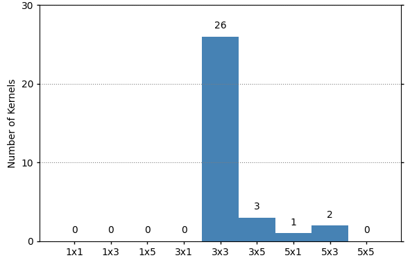
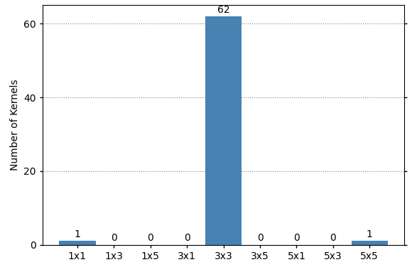
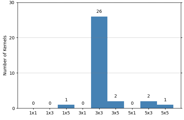
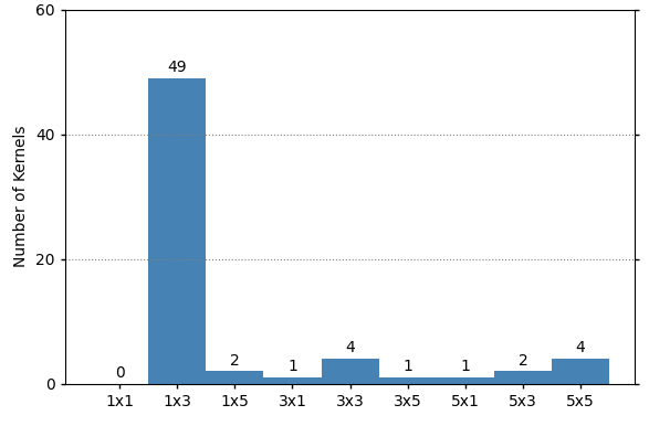
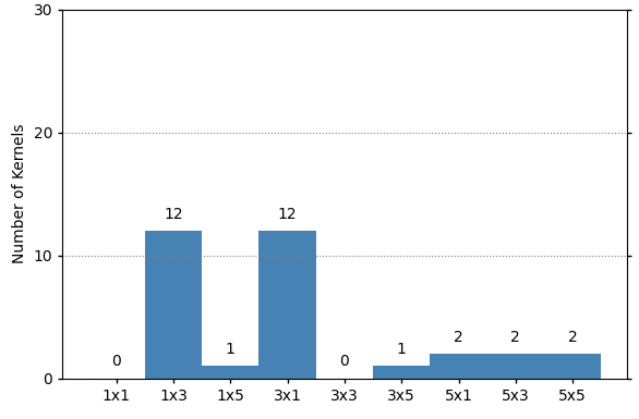
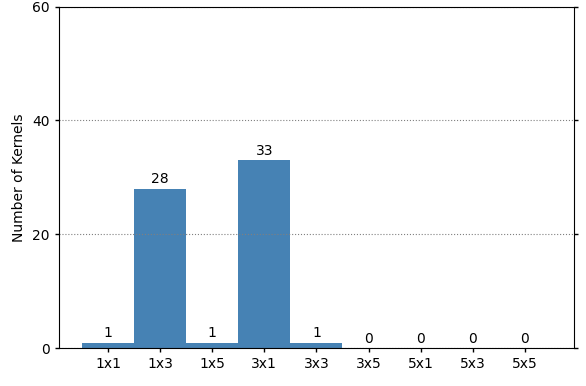
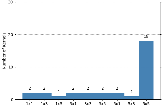
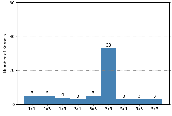
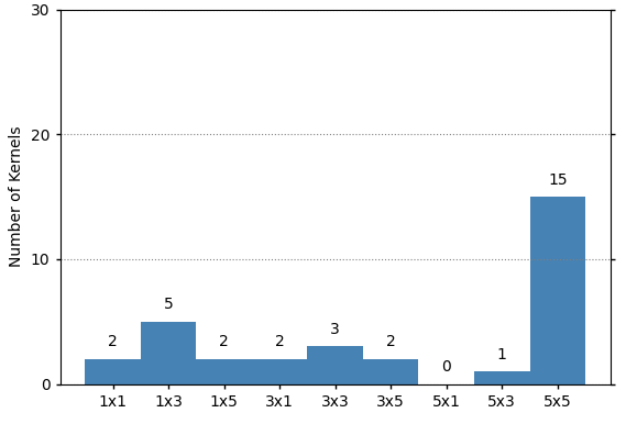
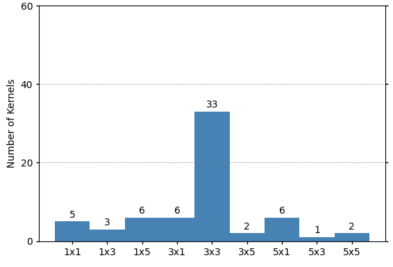
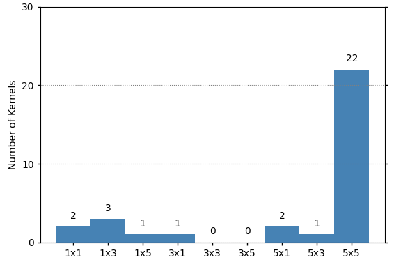
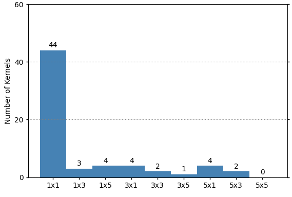
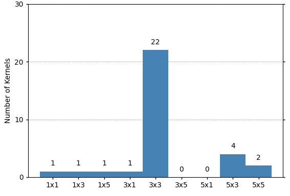
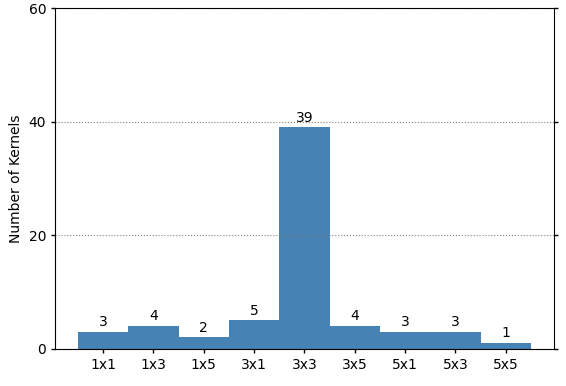
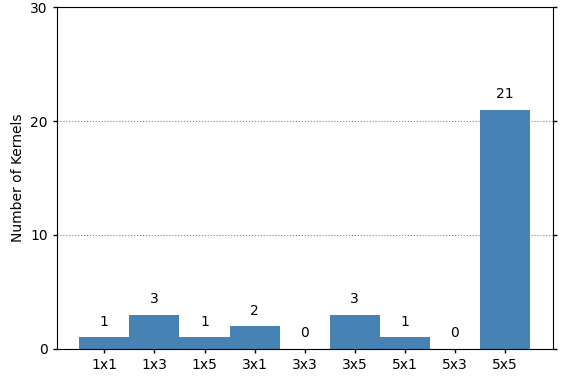
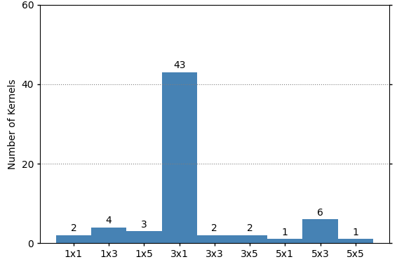
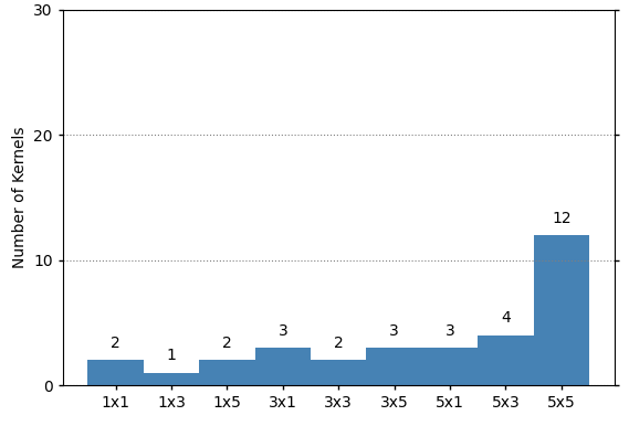
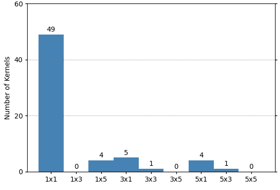
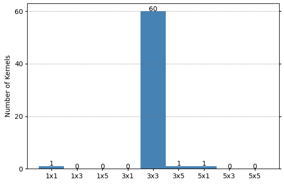
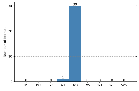
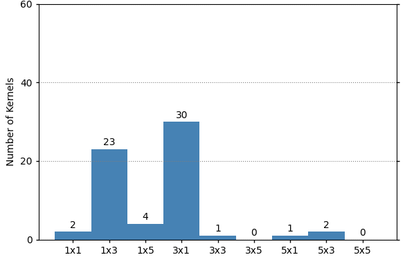
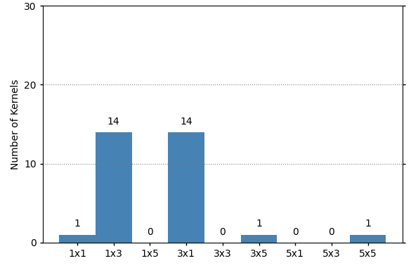
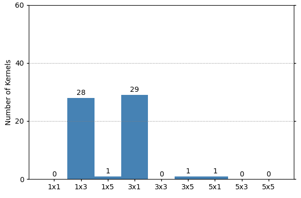
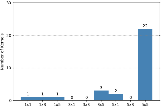
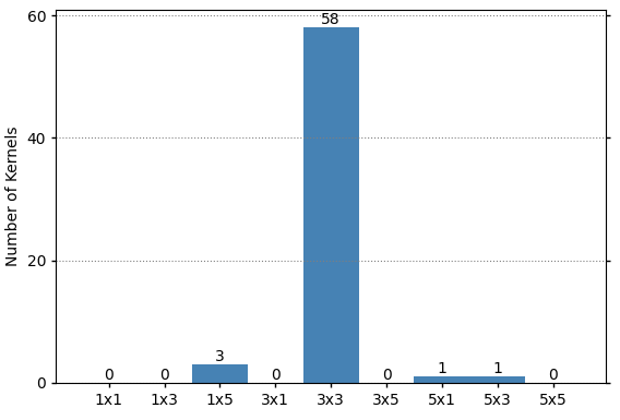
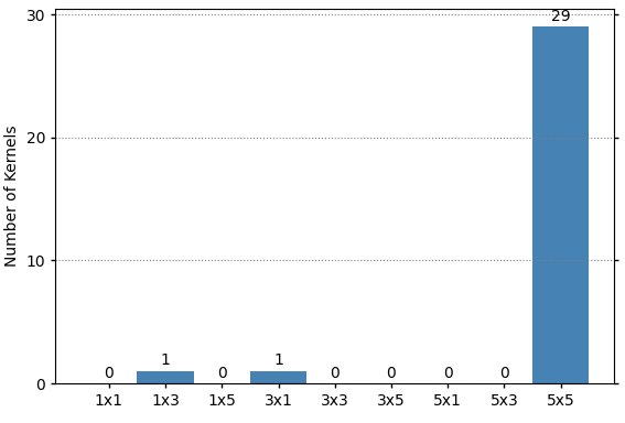
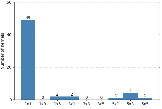
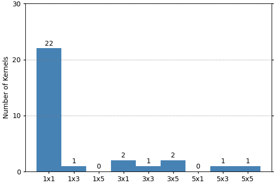
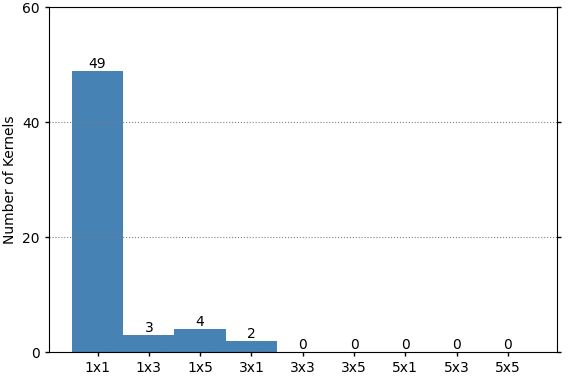
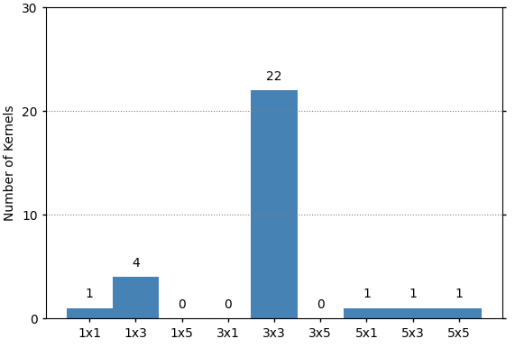
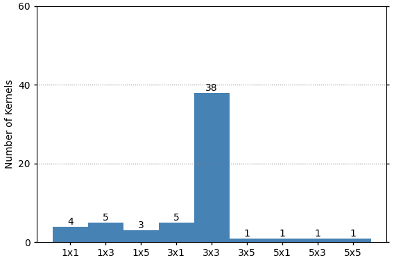
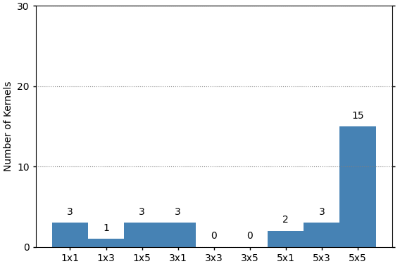
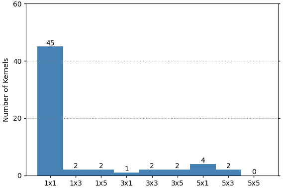
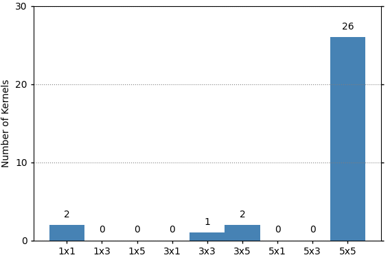
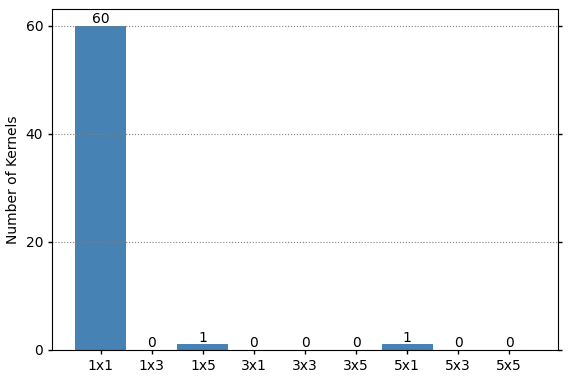
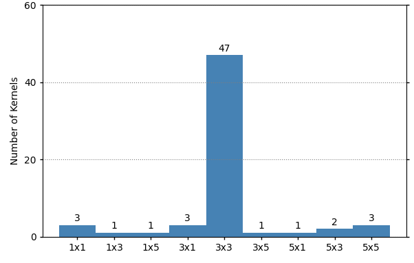
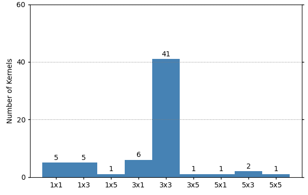
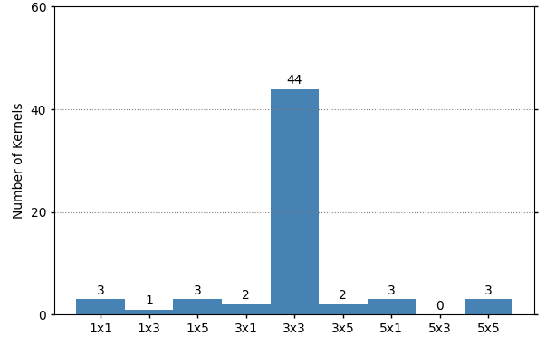
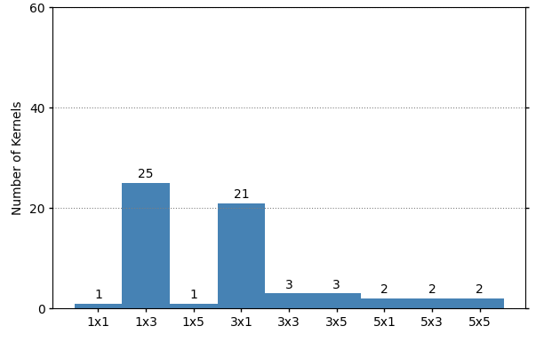
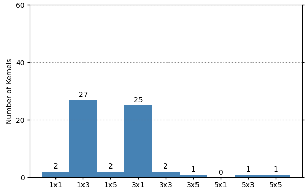
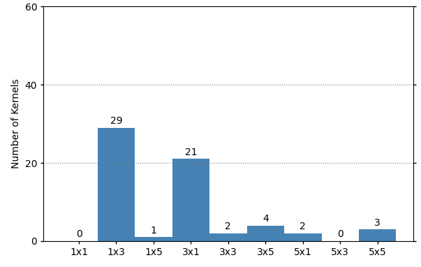
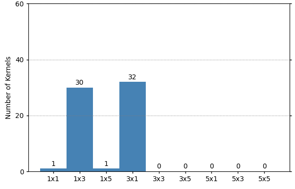
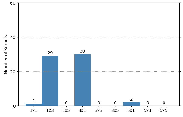
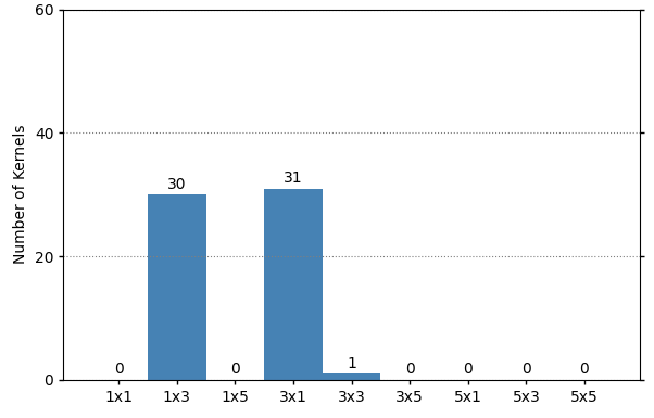
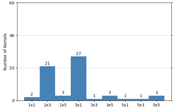
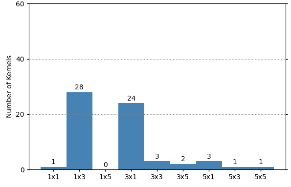
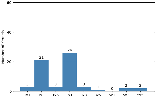
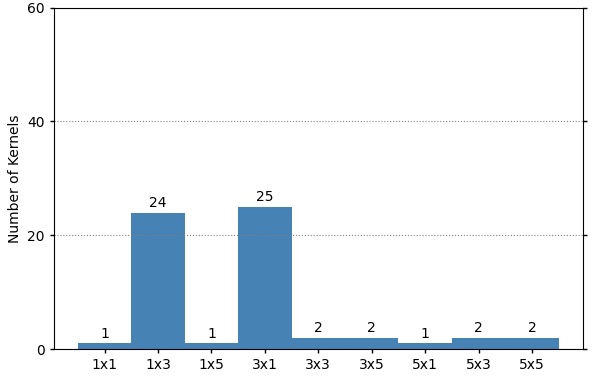
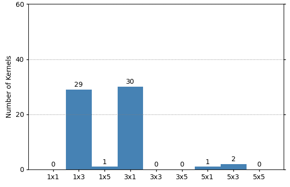
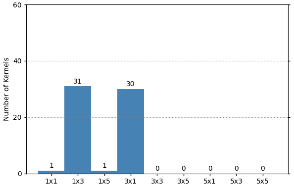
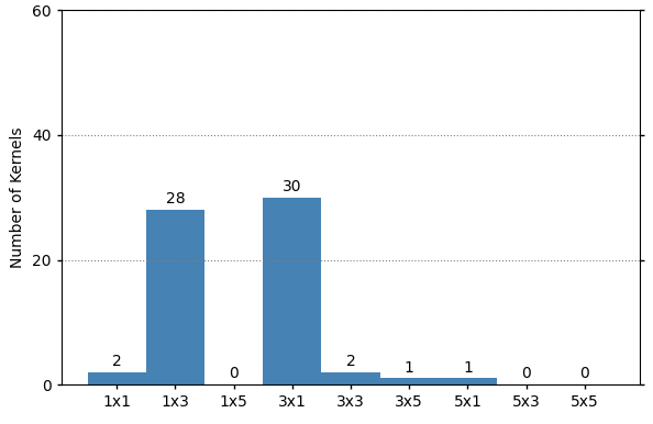
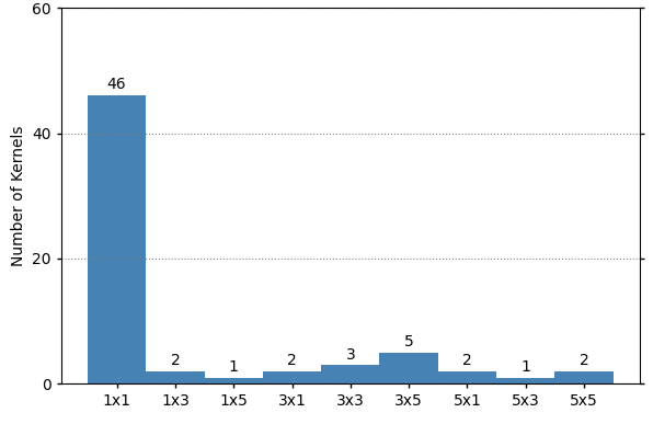
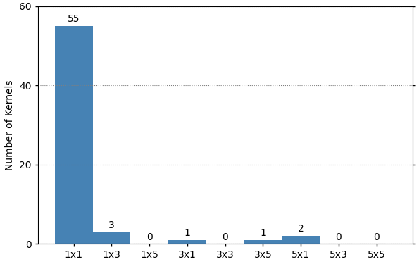
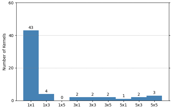
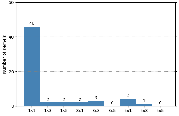
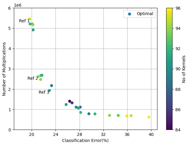
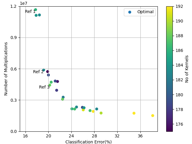
Fig. 18a illustrates optimal solutions for the benchmark network on the CIFAR-10 dataset. Compared with the two-objective optimisation in the previous sections, a number of kernels in both convolutional layers have been removed by the three-objective optimisation method. By removing some of the kernels, optimising for the three objectives can further reduce the number of multiplications that are required to process the CNN without compromising significantly on classification accuracy. In addition, Fig. 18b shows the kernel distributions of three reference points for both convolutional layers after applying the proposed method. The first reference point is the network architecture which features the highest classification accuracy achieved by the proposed method. The second reference point is the one that still features good classification performance while uses less computational resources than the first reference point. Notably, it also outperforms the benchmark network architecture in this case. The third reference point is the best trade-off (closest to origin) between number of multiplications, number of kernels and classification accuracy after optimisation. Details of kernels usage of three reference architectures can be viewed in Appendix B.
These networks from the three reference points have been re-trained for 100 epochs on the whole training set of CIFAR-10, i.e. 50,000 images for training, and the classification accuracy is evaluated on the test set which contains 10,000 examples. It can be seen from Fig. 18b, Ref 1 contains a majority of kernels, and combined with a small number of unconventional kernels in both convolution layers. For Ref 2 and Ref 3, these networks mainly involve kernels in the first convolutional layer and also make use of kernels with different sizes. In the second convolution layer of Ref 2, most of kernels are replaced by kernels and kernels. This replacement is the main reason for Ref 2’s significant reduction in computational resource compared Ref 1 and only has a small impact on its classification accuracy. Both the Ref 1 and Ref 2 outperform the benchmark CNN describe in Fig. 14. Ref 3 provide the best trade-off between the number of multiplications, number of kernels and classification accuracy. It can be seen that Ref 3 uses 8.03x fewer multiplications than the benchmark CNN with only 1.64% increases of classification error. Both convolutional layers in Ref 3 involve kernels and kernels at the most.
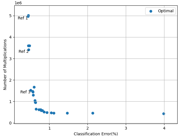
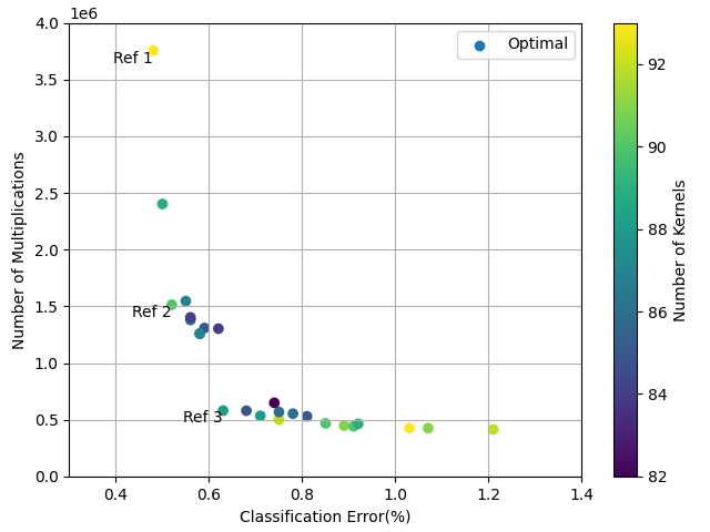
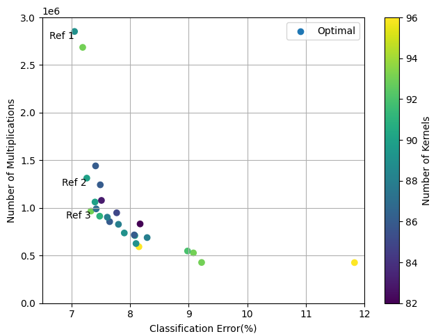
The three-objective optimisation has also been tested on MNIST and Fashion-MNIST datasets. The optimisation results of the benchmark CNN on MNIST dataset are shown in Fig. 17a and Fig. 17b illustrates the optimisation results for the benchmark CNN on MNIST and Fashion-MNIST, respectively. Details of kernels usage of three reference architectures in each dataset can be viewed in Appendix B.
IV-D Results on Deeper CNNs
As shown in the results of the experiments, the proposed method demonstrates significant improvements in reducing computational resource consumption in convolutional layers. The effectiveness of the proposed method is now evaluated on deeper CNNs to give some indication of scalability. The benchmark architecture that is used in these experiments are three and four convolutional layer architectures. Based on the previous experiments, the benchmark architectures have been modified to use kernels in each convolutional layer as a starting point.
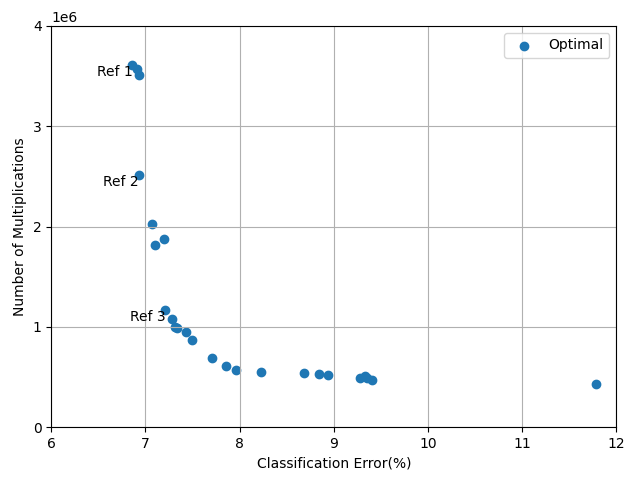
The three-layer benchmark architecture consists of three convolutional layers, each layer includes 64 convolution kernels. Each convolutional layer is followed by a max pooling operation. The four-layer benchmark architecture has four convolutional layers, each layer also includes 64 convolution kernels. The max polling operations are applied at the end of the first, second and fourth convolutional layers. After the convolutional layers, there is a fully-connected layer with a total of 512 neurons and a sofmax operation is used to predict the classification. These experiments use three objectives to evaluate the fitness, which are number of multiplications, Top-1 classification error and number of convolution kernels. During optimsation, all networks are trained on CIFAR-10 dataset for 30 epochs and the evolutionary loop is set to run 100 generations with population size of 25. Three reference architectures from each experiment are selected and re-trained for 100 epochs on the whole training set of CIFAR-10 and the classification accuracy is evaluated on the test set. The first reference point features the highest classification accuracy in the solution set after optimisation. The second reference point involves fewer multiplications and still features good classification accuracy. The third reference point is the best trade-off solution (closest to origin) between number of multiplications, number of kernels, and classification accuracy. Table. III illustrates the results of three reference architectures that are found by the proposed method for each benchmark. Fig. 19 and Fig. 20 show the optimal results that are found by the proposed method on CIFAR-10 dataset. Details of kernels usage of three reference architectures can be viewed in Appendix C.
| Model | Referent Network | Acc. improve | Reduction in Mults. |
|---|---|---|---|
| three-layers | Ref 1 | 0.16% | 1.17x |
| Ref 2 | -1.03% | 2.31x | |
| Ref 3 | -2.44% | 3.06x | |
| four-layers | Ref 1 | -0.32% | 2.13x |
| Ref 2 | -0.95% | 2.90x | |
| Ref 3 | -2.46% | 4.42x |
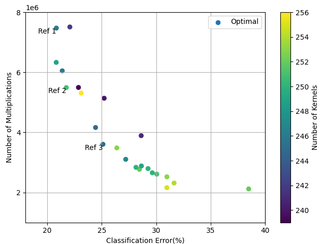
As shown in Table. III, the proposed method still can outperform the network using only conventional convolutions, which is the standard setting in modern CNN architecture design. As the results show, the number of multiplications in convolutional layers of the three-layer CNN achieves 1.17x less than the benchmark architecture, while the Top-1 accuracy increases 0.16%. For four-layer CNN, the proposed method achieve 2.13x saving in number of multiplication with 0.32% decrease in Top-1 accuracy. This demonstrates the capability of the proposed method to be applied to deeper CNN architectures.
In order to validate the performance of the optimised architecture by the proposed method on various datasets, the best trade-off architectures, Ref 3 from Fig 19a and Fig. 20, from both three-layer and four-layer networks have been selected to train on MNIST and Fashion-MNIST datasets. These two datasets contain grey-scale images, so that, benchmark CNN and selected networks are configured as one input channel with input images. Two networks are trained by using Adam optimiser for 100 epochs with initial learning rate of 0.001 and the learning rate is reduced by a factor of 10 at 30th epoch. The experimental results have been reported in Table. IV.
| Model | Dataset | Original Acc. | Optimised Acc. |
|---|---|---|---|
| three-layers | MNIST | 99.08% | 99.13% |
| Fashion-MNIST | 92.64% | 93.06% | |
| four-layers | MNIST | 99.14% | 99.04% |
| Fashion-MNIST | 92.72% | 92.53% |
V Conclusion
In this article, we proposed a generic Multi-objective Evolutionary Algorithm (MOEA)-based approach for optimising the size and efficiency of CNN architectures by introducing unconventional (non-square) kernel shapes and combining different sizes of convolution kernels. The proposed method automatically generates combinations of these unconventional kernels that are used to replace the set of one-size square convolution kernels produced by a conventional approach. The optimisation by MOEA provides a trade-off solution space between computational resources and classification accuracy, which is unique to such algorithms. The results show that a significant reduction in the computational resource consumption with negligible sacrifice of (and sometimes slightly increased) performance.
Moreover, in order to put further emphasis on reduction of the computational resources, the proposed method can reduce the number of kernels used in each convolutional layer in addition to replacing the square kernels by the set of unconventional kernels. The proposed method has been tested on MNIST, Fashion-MNIST and CIFAR-10 datasets with CNN architectures of various depth. As can be seen from the results, the proposed method shows large improvements on computational resource consumption, sometimes with increases in classification accuracy, compared with conventional design of convolutional layers. Trading off accuracy with computational complexity of resource consumption in CNNs running in resource-constrained environments is a real-world problem. This significant reduction of computational resources allows deep CNN architectures to be efficiently implemented on many resource-constrained platforms, such as Field Programmable Gate Arrays (FPGAs) and embedded devices. The methodology of adapting kernel shapes shows premise to be generalised in the future.
Acknowledgement
This project was undertaken on the Viking Cluster, which is a high performance compute facility provided by the University of York. We are grateful for computational support from the University of York High Performance Computing service, Viking and the Research Computing team.
References
- Bergstra and Bengio, (2012) Bergstra, J. and Bengio, Y. (2012). Random search for hyper-parameter optimization. Journal of Machine Learning Research, 13(Feb):281–305.
- Canziani et al., (2016) Canziani, A., Paszke, A., and Culurciello, E. (2016). An analysis of deep neural network models for practical applications. arXiv preprint arXiv:1605.07678.
- Coello, (2001) Coello, C. A. C. (2001). A short tutorial on evolutionary multiobjective optimization. In International Conference on Evolutionary Multi-Criterion Optimization, pages 21–40. Springer.
- Coello, (2006) Coello, C. C. (2006). Evolutionary multi-objective optimization: a historical view of the field. IEEE computational intelligence magazine, 1(1):28–36.
- Deb et al., (2002) Deb, K., Pratap, A., Agarwal, S., and Meyarivan, T. (2002). A fast and elitist multiobjective genetic algorithm: Nsga-ii. IEEE transactions on evolutionary computation, 6(2):182–197.
- Denil et al., (2013) Denil, M., Shakibi, B., Dinh, L., De Freitas, N., et al. (2013). Predicting parameters in deep learning. In Advances in neural information processing systems, pages 2148–2156.
- Denton et al., (2014) Denton, E. L., Zaremba, W., Bruna, J., LeCun, Y., and Fergus, R. (2014). Exploiting linear structure within convolutional networks for efficient evaluation. In Advances in neural information processing systems, pages 1269–1277.
- Dernoncourt and Lee, (2016) Dernoncourt, F. and Lee, J. Y. (2016). Optimizing neural network hyperparameters with gaussian processes for dialog act classification. In 2016 IEEE Spoken Language Technology Workshop (SLT), pages 406–413. IEEE.
- Ding et al., (2019) Ding, X., Guo, Y., Ding, G., and Han, J. (2019). Acnet: Strengthening the kernel skeletons for powerful cnn via asymmetric convolution blocks. In Proceedings of the IEEE International Conference on Computer Vision, pages 1911–1920.
- Gersho and Gray, (2012) Gersho, A. and Gray, R. M. (2012). Vector quantization and signal compression, volume 159. Springer Science & Business Media.
- Gong et al., (2014) Gong, Y., Liu, L., Yang, M., and Bourdev, L. (2014). Compressing deep convolutional networks using vector quantization. arXiv preprint arXiv:1412.6115.
- Goodfellow et al., (2016) Goodfellow, I., Bengio, Y., and Courville, A. (2016). Deep learning. MIT press.
- (13) Guo, Y., Liu, Y., Oerlemans, A., Lao, S., Wu, S., and Lew, M. S. (2016a). Deep learning for visual understanding: A review. Neurocomputing, 187:27–48.
- (14) Guo, Y., Yao, A., and Chen, Y. (2016b). Dynamic network surgery for efficient dnns. In Advances In Neural Information Processing Systems, pages 1379–1387.
- Han et al., (2015) Han, S., Mao, H., and Dally, W. J. (2015). Deep compression: Compressing deep neural networks with pruning, trained quantization and huffman coding. arXiv preprint arXiv:1510.00149.
- Hanson and Pratt, (1989) Hanson, S. J. and Pratt, L. Y. (1989). Comparing biases for minimal network construction with back-propagation. In Advances in neural information processing systems, pages 177–185.
- He et al., (2016) He, K., Zhang, X., Ren, S., and Sun, J. (2016). Deep residual learning for image recognition. In Proceedings of the IEEE conference on computer vision and pattern recognition, pages 770–778.
- Jaderberg et al., (2014) Jaderberg, M., Vedaldi, A., and Zisserman, A. (2014). Speeding up convolutional neural networks with low rank expansions. arXiv preprint arXiv:1405.3866.
- Jin et al., (2014) Jin, J., Dundar, A., and Culurciello, E. (2014). Flattened convolutional neural networks for feedforward acceleration. arXiv preprint arXiv:1412.5474.
- Kim et al., (2017) Kim, Y.-H., Reddy, B., Yun, S., and Seo, C. (2017). Nemo: Neuro-evolution with multiobjective optimization of deep neural network for speed and accuracy. In JMLR: Workshop and Conference Proceedings, volume 1, pages 1–8.
- Kingma and Ba, (2014) Kingma, D. P. and Ba, J. (2014). Adam: A method for stochastic optimization. arXiv preprint arXiv:1412.6980.
- Krizhevsky and Hinton, (2010) Krizhevsky, A. and Hinton, G. (2010). Convolutional deep belief networks on cifar-10. Unpublished manuscript, 40(7):1–9.
- Krizhevsky et al., (2012) Krizhevsky, A., Sutskever, I., and Hinton, G. E. (2012). Imagenet classification with deep convolutional neural networks. In Advances in neural information processing systems, pages 1097–1105.
- Larochelle et al., (2007) Larochelle, H., Erhan, D., Courville, A., Bergstra, J., and Bengio, Y. (2007). An empirical evaluation of deep architectures on problems with many factors of variation. In Proceedings of the 24th international conference on Machine learning, pages 473–480.
- LeCun et al., (1998) LeCun, Y., Bottou, L., Bengio, Y., Haffner, P., et al. (1998). Gradient-based learning applied to document recognition. Proceedings of the IEEE, 86(11):2278–2324.
- LeCun et al., (2010) LeCun, Y., Cortes, C., and Burges, C. (2010). Mnist handwritten digit database. ATT Labs [Online]. Available: http://yann. lecun. com/exdb/mnist, 2.
- Miikkulainen et al., (2019) Miikkulainen, R., Liang, J., Meyerson, E., Rawal, A., Fink, D., Francon, O., Raju, B., Shahrzad, H., Navruzyan, A., Duffy, N., et al. (2019). Evolving deep neural networks. In Artificial Intelligence in the Age of Neural Networks and Brain Computing, pages 293–312. Elsevier.
- Miller and Harding, (2008) Miller, J. F. and Harding, S. L. (2008). Cartesian genetic programming. In Proceedings of the 10th annual conference companion on Genetic and evolutionary computation, pages 2701–2726.
- Moriarty and Miikkulainen, (1998) Moriarty, D. E. and Miikkulainen, R. (1998). Hierarchical evolution of neural networks. In 1998 IEEE International Conference on Evolutionary Computation Proceedings. IEEE World Congress on Computational Intelligence (Cat. No. 98TH8360), pages 428–433. IEEE.
- Morse and Stanley, (2016) Morse, G. and Stanley, K. O. (2016). Simple evolutionary optimization can rival stochastic gradient descent in neural networks. In Proceedings of the Genetic and Evolutionary Computation Conference 2016, pages 477–484.
- Rasmussen, (2003) Rasmussen, C. E. (2003). Gaussian processes in machine learning. In Summer School on Machine Learning, pages 63–71. Springer.
- Real et al., (2017) Real, E., Moore, S., Selle, A., Saxena, S., Suematsu, Y. L., Tan, J., Le, Q. V., and Kurakin, A. (2017). Large-scale evolution of image classifiers. In Proceedings of the 34th International Conference on Machine Learning-Volume 70, pages 2902–2911. JMLR. org.
- Ren et al., (2017) Ren, S., He, K., Girshick, R., and Sun, J. (2017). Faster r-cnn: Towards real-time object detection with region proposal networks. IEEE transactions on pattern analysis and machine intelligence, 39(6):1137.
- Sironi et al., (2014) Sironi, A., Tekin, B., Rigamonti, R., Lepetit, V., and Fua, P. (2014). Learning separable filters. IEEE transactions on pattern analysis and machine intelligence, 37(1):94–106.
- Snoek et al., (2012) Snoek, J., Larochelle, H., and Adams, R. P. (2012). Practical bayesian optimization of machine learning algorithms. In Advances in neural information processing systems, pages 2951–2959.
- Stanley et al., (2009) Stanley, K. O., D’Ambrosio, D. B., and Gauci, J. (2009). A hypercube-based encoding for evolving large-scale neural networks. Artificial life, 15(2):185–212.
- Stanley and Miikkulainen, (2002) Stanley, K. O. and Miikkulainen, R. (2002). Efficient evolution of neural network topologies. In Proceedings of the 2002 Congress on Evolutionary Computation. CEC’02 (Cat. No. 02TH8600), volume 2, pages 1757–1762. IEEE.
- Su et al., (2018) Su, J., Faraone, J., Liu, J., Zhao, Y., Thomas, D. B., Leong, P. H., and Cheung, P. Y. (2018). Redundancy-reduced mobilenet acceleration on reconfigurable logic for imagenet classification. In International Symposium on Applied Reconfigurable Computing, pages 16–28. Springer.
- Suganuma et al., (2017) Suganuma, M., Shirakawa, S., and Nagao, T. (2017). A genetic programming approach to designing convolutional neural network architectures. In Proceedings of the Genetic and Evolutionary Computation Conference, pages 497–504.
- Sullivan, (1996) Sullivan, G. J. (1996). Efficient scalar quantization of exponential and laplacian random variables. IEEE Transactions on information theory, 42(5):1365–1374.
- Sun et al., (2018) Sun, Y., Xue, B., Zhang, M., and Yen, G. G. (2018). Automatically designing cnn architectures using genetic algorithm for image classification. arXiv preprint arXiv:1808.03818.
- Swersky et al., (2013) Swersky, K., Snoek, J., and Adams, R. P. (2013). Multi-task bayesian optimization. In Advances in neural information processing systems, pages 2004–2012.
- Szegedy et al., (2015) Szegedy, C., Liu, W., Jia, Y., Sermanet, P., Reed, S., Anguelov, D., Erhan, D., Vanhoucke, V., and Rabinovich, A. (2015). Going deeper with convolutions. In Proceedings of the IEEE conference on computer vision and pattern recognition, pages 1–9.
- Szegedy et al., (2016) Szegedy, C., Vanhoucke, V., Ioffe, S., Shlens, J., and Wojna, Z. (2016). Rethinking the inception architecture for computer vision. In Proceedings of the IEEE conference on computer vision and pattern recognition, pages 2818–2826.
- Verbancsics and Harguess, (2015) Verbancsics, P. and Harguess, J. (2015). Image classification using generative neuro evolution for deep learning. In 2015 IEEE winter conference on applications of computer vision, pages 488–493. IEEE.
- Xiao et al., (2017) Xiao, H., Rasul, K., and Vollgraf, R. (2017). Fashion-mnist: a novel image dataset for benchmarking machine learning algorithms. arXiv preprint arXiv:1708.07747.
- Xie and Yuille, (2017) Xie, L. and Yuille, A. (2017). Genetic cnn. In Proceedings of the IEEE international conference on computer vision, pages 1379–1388.
- Yu and Koltun, (2015) Yu, F. and Koltun, V. (2015). Multi-scale context aggregation by dilated convolutions. arXiv preprint arXiv:1511.07122.
- Zhao et al., (2019) Zhao, Z.-Q., Zheng, P., Xu, S.-t., and Wu, X. (2019). Object detection with deep learning: A review. IEEE transactions on neural networks and learning systems, 30(11):3212–3232.
Appendix A Two-Objective Optimisation
These figures are for two-objective optimisation experiments in Section 4.2.
-
•
Fig. 10 shows the optimisation result by the proposed method and a brief plot of kernel shape distributions of three reference architectures from the optimisation result of benchmark CNN on CIFAR-10 dataset.
-
•
Fig. 11 shows the optimisation results by the proposed method and a brief plot of kernel shape distributions of three reference architectures from the optimisation result of benchmark CNN on MNIST dataset.
-
•
Fig. 12 shows the optimisation results by the proposed method and a brief plot of kernel shape distributions of three reference architectures from the optimisation results of benchmark CNN on Fashion-MNIST dataset.
-
•
Fig. 13 gives the details of kernel usage of three reference architectures from the optimisation results of benchmark CNN on CIFAR-10 dataset.
-
•
Fig. 14 gives the details of kernel usage of three reference architectures from the optimisation results of benchmark CNN on MNIST dataset.
-
•
Fig. 15 gives the details of kernel usage of three reference architectures from the optimisation results of benchmark CNN on Fashion-MNIST dataset.
Appendix B Three-Objective Optimisation
These figures are for three-objective optimisation experiments in Section 4.3.
-
•
Fig. 16 gives the details of kernel usage of three reference architectures from the optimisation results of benchmark CNN on CIFAR-10 dataset.
-
•
Fig. 17 gives the details of kernel usage of three reference architectures from the optimisation results of benchmark CNN on MNIST dataset.
-
•
Fig. 18 gives the details of kernel usage of three reference architectures from the optimisation results of benchmark CNN on Fashion-MNIST dataset.
Appendix C Three-layer and Four-layer Networks Optimisation
These figures are for three-objective optimisation of deeper CNNs with three layers. Experiments are in Section 4.4.
-
•
Fig. 19 shows the details of kernel usage of first reference point, Ref 1, from the optimisation results of three-layer network on CIFAR-10 dataset.
-
•
Fig. 20 shows the details of kernel usage of second reference point, Ref 2, from the optimisation results of three-layer network on CIFAR-10 dataset.
-
•
Fig. 21 shows the details of kernel usage of third reference point, Ref 3, from the optimisation results of three-layer network on CIFAR-10 dataset.
These figures are for three-objective optimisation of deeper CNNs with four layers. Experiments are in Section 4.4.
-
•
Fig. 22 shows the details of kernel usage of first reference point, Ref 1, from the optimisation results of four-layer network on CIFAR-10 dataset.
-
•
Fig. 23 shows the details of kernel usage of second reference point, Ref 2, from the optimisation results of four-layer network on CIFAR-10 dataset.
-
•
Fig. 24 shows the details of kernel usage of third reference point, Ref 3, from the optimisation results of four-layer network on CIFAR-10 dataset.